Microwave multiphoton conversion via coherently driven permanent dipole systems

Abstract

We investigate the multiphoton quantum dynamics of a leaking single-mode quantized cavity field coupled with a resonantly driven two-level system possessing permanent dipoles. The frequencies of the interacting subsystems are being considered very different, e.g., microwave ranges for the cavity and optical domains for the frequency of the two-level emitter, respectively. In this way, the emitter couples to the resonator mode via its diagonal dipole moments only. Furthermore, the generalized Rabi frequency resulting form the external coherent driving of the two-level subsystem is assumed as well different from the resonator’s frequency or its multiples. As a consequence, this highly dispersive interaction regime is responsible for the cavity multiphoton quantum dynamics and photon conversion from optical to microwave ranges, respectively.

I Introduction

Frequency conversion processes where an input light beam can be converted at will into an output beam of a different frequency are very relevant nowadays due to various feasible quantum applications aps ; aps1 ; aps2 ; aps3 . Among the first demonstrations of this effect is the experiment reported in exp1 promising developments of tunable sources of quantum light. From this reason, single-photon upconversion from a quantum dot preserving the quantum features was demonstrated in exp2 . Experimental demonstration of strong coupling between telecom (1550 nm) and visible (775 nm) optical modes on an aluminum nitride photonic chip was demonstrated as well, in Ref. exp3 . Even bigger frequency differences can be generated. For instance, an experimental demonstration of converting a microwave field to an optical field via frequency mixing in a cloud of cold ⁸⁷Rb atoms was reported in exp4 . Earlier theoretical studies have demonstrated frequency downconversion in pumped two-level systems with broken inversion symmetry theor1 ; theor2 . Furthermore, single- and multiphoton frequency conversion via ultra-strong coupling of a two-level emitter to two resonators was theoretically predicted in theor3 . Although multiquanta processes are being investigated already for a long period of time, recently have attracted considerable attention as well. This is mainly due to potential application of these processes to quantum technologies related to quantum lithography qlit or novel sources of light nsource , etc. rew ; ffilter ; fedr . Additionaly, optomechanically multiphonon induced transparency of x-rays via optical control was demonstrated in wen-te while strongly correlated multiphonon emission in an acoustical cavity coupled to a driven two-level quantum dot was demonstrated in Ref. nori , respectively.

However, most of the frequency conversion investigations refer to resonant processes. In this context, here, we shall demonstrate a photon conversion scheme involving non-resonant multiphoton effects, respectively. Actually, we investigate frequency downconversion processes via a resonantly laser-pumped two-level emitter possessing permanent diagonal dipoles, $d_{\alpha\alpha}\not=0$ with $\alpha\in\{1,2\}$, and embedded in a single-mode quantized resonator, see Fig. (1). The frequency of the two-level emitter is assumed to be in the optical range and it is significantly different from the cavity frequency which may be in the microwave domain, for instance. Therefore, the two-level emitter naturally couples to the resonator through its permanent dipoles only. The cavity’s frequency or its multiples differs as well from the generalized Rabi frequency arising due to resonant and coherent external driving of the two-level emitter. As a result, this highly dispersive interaction regime leads to multiphoton absorption-emission processes in the resonator mode mediated by the corresponding damping effects, i.e., emitter’s spontaneous emission and the photon leaking through the cavity walls, respectively. We have obtained the corresponding cavity photon quantum dynamics in the steady state and demonstrated the feasibility to generate a certain multiphoton superposition state with high probability, and at different frequencies than that of the input external coherent pumping. The multiquanta nature of the final cavity state can be demonstrated via the second-order photon-photon correlation function.

The advantage of our scheme consists in availability of its constituents, having $d_{22}\not=d_{11}$, such as asymmetrical two-level quantum dots twoa ; mqd1 ; mqd2 and molecules kov ; alt1 ; alt2 , or, equivalently, spin or quantum circuits alt3 ; alt4 , together with the technological progress towards their coupling to various resonators. As feasible applications of our results one may consider the possibility to couple distant real or artificial atoms having transition frequencies in the microwave domain via the multiphoton state generated by the developed model here, see also dist_at . Various entangled states enth1 ; enth2 ; basharov ; ficek of distant emitters can be generated then. Another option, for instance, would be to investigate the quantum thermodynamic performances quth of distant qubit systems interconnected through the microwave multiphoton field described here.

The article is organized as follows. In Sec. II we apply the developed analytical approach to the system of interest and describe it, while in Sec. III we analyze the obtained results. The summary is given in Sec. IV.

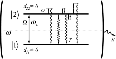
Figure 1: The schematic of the model: A coherently pumped two-level emitter couples with a single-mode resonator of frequency $\omega$ via its non-zero diagonal dipoles, $d_{\alpha\alpha}$, with $\alpha\in\{1,2\}$. Here, $\Omega$ is the corresponding Rabi frequency due to the off-diagonal dipole moment $d_{21}$ whereas $\omega_{L}$, $\omega_{L}\gg\omega$, is the frequency of the resonantly applied external field. The emitter-resonator coupling strength is denoted by $g$, while $\kappa$ is the resonator’s decay rate. Also, are sketched some processes which may occur, namely, emission/absorption of a cavity photon (or two, three, etc.) followed by the spontaneous decay $\gamma$.

II Analytical framework

The master equation describing the interaction of a two-level emitter, possessing permanent diagonal dipoles, with a classical coherent electromagnetic field of frequency $\omega_{L}$ as well as with a quantized single mode resonator of frequency $\omega$, with $\omega\ll\omega_{L}$ (see Fig. 1), and damped via the corresponding environmental reservoirs in the Born-Markov approximations agar ; szu ; gxl_b , is:

$$\frac{d}{dt}\rho(t) + \frac{i}{\hbar}[H,\rho]=-\frac{\gamma}{2}[S^{+},S^{-}\rho]-\frac{\kappa}{2}(1+\bar{n})[b^{\dagger},b\rho]$$ (1)

$$- \frac{\kappa}{2}\bar{n}[b,b^{\dagger}\rho]+H.c..$$

Here, $\gamma$ is the single-emitter spontaneous decay rate, whereas $\kappa$ is the corresponding boson-mode’s leaking rate with $\bar{n}$ = $\bigl{[}\exp[\hbar\omega/(k_{B}T)]-1\bigr{]}^{-1}$ being the mean resonator’s photon number due to the environmental thermostat at temperature $T$, and $k_{B}$ is the Boltzmann constant. The two-level system may have the transition frequency in the optical domain, whereas the single-mode cavity frequency may lay in the microwave range, respectively. The wavevector of the coherent applied field is perpendicular to the cavity axis. In the Eq. (1), the bare-state emitter’s operators $S^{+}=|2\rangle\langle 1|$ and $S^{-}=[S^{+}]^{\dagger}$ obey the commutation relations for su(2) algebra, namely, $[S^{+},S^{-}]=2S_{z}$ and $[S_{z},S^{\pm}]=\pm S^{\pm}$, where $S_{z}=(|2\rangle\langle 2|-|1\rangle\langle 1|)/2$ is the bare-state inversion operator. $|2\rangle$ and $|1\rangle$ are the excited and ground state of the emitter, respectively, while $b^{\dagger}$ and $b$ are the creation and the annihilation operator of the electromagnetic field (EMF) in the resonator, and satisfy the standard bosonic commutation relations, i.e., $[b,b^{\dagger}]=1$, and $[b,b]=[b^{\dagger},b^{\dagger}]=0$. The Hamiltonian characterizing the respective coherent evolution of the considered compound system is (see Appendix A):

$$H=\hbar\omega b^{\dagger}b+\hbar\Delta S_{z}-\hbar\Omega(S^{+}+S^{-})+\hbar gS_{z}(b^{\dagger}+b).$$ (2)

In the Hamiltonian (2), the first two components describe the free energies of the cavity electromagnetic field and the two-level emitter, respectively, with $\Delta=\omega_{21}-\omega_{L}$ being the detuning of the emitter transition frequency $\omega_{21}$ from the laser one. The last two terms depict, respectively, the laser interaction with the two-level system and the emitter-cavity interaction. $\Omega$ and $g$ are the corresponding coupling strengths. Note at this stage that while the Rabi frequency $\Omega$ is proportional to the off-diagonal dipole moment $d_{21}$, the emitter-cavity coupling is proportional to the diagonal dipole moments, i.e. $g\propto(d_{22}-d_{11})$. The interaction of the external coherent electromagnetic field with permanent dipoles is omitted here as being rapidly oscillating. From the same reason, the emitter-cavity interaction described by the usual Jaynes-Cummings Hamiltonian, proportional to $d_{21}$, is neglected as well here, see Appendix A.

In what follows, we perform a spin rotation enaki ; saiko ; mekPRA2020 ,

$$U(\chi)=\exp\bigl{[}2i\chi S_{y}\bigr{]},$$ (3)

where $S_{y}=(S^{+}-S^{-})/2i$ and $2\chi=\arctan{[2\Omega/\bar{\Delta}]}$ with $\bar{\Delta}=\Delta+g(b^{\dagger}+b)$, diagonalizing the last three terms of the Hamiltonian (2). This action will lead to new quasi-spin operators, i.e. $R_{z}$ and $R^{\pm}$, defined via the old emitter’s operators in the following way

$$R_{z} = S_{z}\cos{2\chi}-(S^{+}+S^{-})\sin{2\chi}/2,$$

$$R^{+} = S^{+}\cos^{2}{\chi}-S^{-}\sin^{2}{\chi}+S_{z}\sin{2\chi},$$

$$R^{-} = [R^{+}]^{\dagger}.$$ (4)

The new emitter operators $R^{+}=|\bar{2}\rangle\langle\bar{1}|$, $R^{-}=|\bar{1}\rangle\langle\bar{2}|$ and $R_{z}=(|\bar{2}\rangle\langle\bar{2}|-|\bar{1}\rangle\langle\bar{1}|)/2$, describing the transitions and populations among the dressed-states $\{|\bar{2}\rangle,|\bar{1}\rangle\}$, will obey the commutation relations: $[R^{+},R^{-}]=2R_{z}$ and $[R_{z},R^{\pm}]=\pm R^{\pm}$, similarly to the old-basis ones. Respectively, the Hamiltonian (2) transforms to:

$$\bar{H}=\hbar\omega b^{\dagger}b+2\hbar\bar{\Omega}R_{z},$$ (5)

where the operator $\bar{\Omega}=(\bar{\Delta}^{2}/4+\Omega^{2})^{1/2}$, whereas

$$b=\bar{b}-i\eta S_{y}\sum^{\infty}_{k=0}\frac{\eta^{k}}{k!}(\bar{b}^{\dagger}+\bar{b})^{k}\frac{\partial^{k}}{\partial\xi^{k}}\frac{1}{1+\xi^{2}},$$ (6)

with $b^{\dagger}=[b]^{\dagger}$, $\bar{b}=U{b}U^{-1}$, $\bar{b}^{\dagger}=[\bar{b}]^{\dagger}$, and

$$\eta=\frac{g}{2\Omega},~{}~{}{\rm and}~{}~{}\xi=\frac{\Delta}{2\Omega}.$$

Now the expressions (4)-(6) have to be introduced in the master equation (1) and the final equation will be somehow cumbersome. It can be simplified if we perform the secular approximation, i.e., neglect all terms from the master equation oscillating at the generalized Rabi frequency $2\Omega_{0}$, $\Omega_{0}=\Omega\sqrt{1+\xi^{2}}$, and higher one. This is justified if $2\Omega_{0}\gg\{g,\gamma\}$ - the situation considered here.

Thus, in the following, we expand the generalized Rabi frequency $\bar{\Omega}$ in the Taylor series using the small parameter $\eta$, namely,

$$\bar{\Omega}=\Omega_{0}\biggl{\{}1+\frac{\xi\hat{\eta}}{1+\xi^{2}}+\frac{\hat{\eta}^{2}}{2(1+\xi^{2})^{2}}-\frac{\xi\hat{\eta}^{3}}{2(1+\xi^{2})^{3}}+\cdots\biggr{\}},$$

where $\hat{\eta}=\eta(\bar{b}^{\dagger}+\bar{b})$. Then perform a unitary transformation $U(t)=\exp[2i\Omega_{0}R_{z}t]$ in the whole master equation and neglect terms oscillating at the Rabi frequency $2\Omega_{0}$ or higher. Afterwards, perform the operation $\rho_{\bar{\alpha}\bar{\alpha}}=\langle\bar{\alpha}|\rho|\bar{\alpha}\rangle$, $\alpha\in\{1,2\}$, and one can arrive then at the following master equation describing the cavity degrees of freedom only:

$$\frac{d}{dt}\bar{\rho}(t) + \frac{i}{\hbar}[\bar{H},\bar{\rho}]-\frac{\gamma}{4}\{\cos 2\chi\bar{\rho}\cos 2\chi+\sin 2\chi\bar{\rho}\sin 2\chi$$ (7)

$$- \bar{\rho}\}=-\frac{\kappa}{2}(1+\bar{n})[\bar{b}^{\dagger},\bar{b}\bar{\rho}]-\frac{\kappa}{2}\bar{n}[\bar{b},\bar{b}^{\dagger}\bar{\rho}]$$

$$- \frac{\kappa\eta^{2}}{8}(1+2\bar{n})\sum^{\infty}_{k_{1},k_{2}=0}f_{k_{1}}(\eta,\xi)f_{k_{2}}(\eta,\xi)$$

$$\times [(\bar{b}^{\dagger}+\bar{b})^{k_{1}},(\bar{b}^{\dagger}+\bar{b})^{k_{2}}\bar{\rho}]+H.c.,$$

where $\bar{\rho}=\rho_{\bar{1}\bar{1}}+\rho_{\bar{2}\bar{2}}$. Here,

$$f_{k}(\eta,\xi) = \frac{\eta^{k}}{k!}\frac{\partial^{k}}{\partial\xi^{k}}\frac{1}{1+\xi^{2}},$$

$$\sin 2\chi = \frac{\Omega}{\bar{\Omega}}=\sum^{\infty}_{k=0}\frac{\eta^{k}(\bar{b}+\bar{b}^{\dagger})^{k}}{k!}\frac{\partial^{k}}{\partial\xi^{k}}\frac{1}{\sqrt{1+\xi^{2}}},$$

$$\cos 2\chi = \frac{\bar{\Delta}/2}{\bar{\Omega}}=\sum^{\infty}_{k=0}\frac{\eta^{k}(\bar{b}+\bar{b}^{\dagger})^{k}}{k!}\frac{\partial^{k}}{\partial\xi^{k}}\frac{\xi}{\sqrt{1+\xi^{2}}}.$$

Already at this stage one can recognize the multiphoton nature of the cavity electromagnetic field quantum dynamics. Particularly in Eq. (7), the term proportional to $\gamma$ describes the resonator’s multiphoton dynamics accompanied by the spontaneous decay, whereas the components proportional to $\kappa$ characterize the same processes but followed by the cavity decay, respectively, see also Fig. (1).

Using the bosonic operator identity ref_binom

$$(A+B)^{n} = \sum^{n}_{k^{\prime}}\frac{n!}{k^{\prime}!(\frac{n-k^{\prime}}{2})!}\biggl{(}-\frac{C}{2}\biggr{)}^{\frac{n-k^{\prime}}{2}}\sum^{k^{\prime}}_{r=0}\frac{k^{\prime}!}{r!(k^{\prime}-r)!}$$

$$\times A^{r}B^{k^{\prime}-r},$$

where $[A,B]=C$ and $[A,C]=[B,C]=0$, whereas $k^{\prime}$ is odd for an odd $n$ and even for an even $n$ (if, for instance, $n=4$, then $k^{\prime}=\{0,2,4\}$, while if $n=5$, then $k^{\prime}=\{1,3,5\}$, whereas $r=0,1,2,\cdots,k^{\prime}$), one can reduce the master equation (7) to a time-independent equation if one further performs a unitary transformation $V(t)=\exp[i\omega\bar{b}^{\dagger}\bar{b}t]$ and neglects all the terms rotating at frequency $\omega$ and higher. This would also result in avoiding any resonances in the system, i.e., $2\Omega_{0}-s\omega\not=0$, $s\in\{1,2,\cdots\}$. As a consequence, one can obtain a diagonal equation for $P_{n}=\langle n|\bar{\rho}|n\rangle$, with $|n\rangle$ being the Fock state and $n\in\{0,1,2,\cdots\}$, describing the cavity multiphoton quantum dynamics, in the presence of corresponding damping effects, which is computed then numerically here. Notice that the coherent part of the master equation (7), i.e. $[\bar{H},\bar{\rho}]$, does not contribute to the final expression for the photon distribution function $P_{n}$. The reason is that after the performed approximations the Hamiltonian $\bar{H}$ would contain photonic correlators such that $\langle n|[\bar{H},\bar{\rho}]|n\rangle$=$\bar{H}_{n}P_{n}-P_{n}\bar{H}_{n}=0$.

Thus, the cavity photon dynamics has a multiphoton behavior because of the highly dispersive (non-resonant) nature of the interaction among the asymmetrical two-level emitter and cavity field mode. This way, one obtains an output multiphoton flux of microwave photons, although the two-level system is coherently pumped at a different frequency, i.e. with optical photons.

III Results and discussion

In the following, we shall describe the cavity multiphoton quantum dynamics based on the Eq. (7). Particularly, for single-photon non-resonant processes one can obtain the following equation for the photon distribution function, see Appendix B:

$$\frac{d}{dt}P_{n}(t)=-P^{(1)}_{n},$$ (8)

where

$$P^{(1)}_{n} = \biggl{\{}\kappa(1+\bar{n})+\frac{\gamma\eta^{2}}{4(1+\xi^{2})^{2}}\biggr{\}}\biggl{(}nP_{n}-(n+1)P_{n+1}\biggr{)}$$

$$+ \biggl{\{}\kappa\bar{n}+\frac{\gamma\eta^{2}}{4(1+\xi^{2})^{2}}\biggr{\}}\biggl{(}(n+1)P_{n}-nP_{n-1}\biggr{)}.$$

The first line of the above expression for $P^{(1)}_{n}$ describes the photon generation processes, i.e., photons that leave the cavity. The second line corresponds to processes describing photons pumping the cavity mode due to the environmental thermostat and non-resonant external driving, respectively. One can observe that both processes are influenced by the resonant laser pumping of the two-level emitter possessing permanent dipoles. As a consequence, the stationary mean-photon number in the resonator mode is, see Appendix B:

$$\langle\bar{b}^{\dagger}\bar{b}\rangle=\bar{n}+\frac{\gamma\eta^{2}}{4\kappa(1+\xi^{2})^{2}},$$ (9)

whereas its second-order photon-photon correlation function is $g^{(2)}(0)=2$, see the blue long-dashed curves in Fig. (2). Respectively, for two-photon non-resonant processes one has:

$$\frac{d}{dt}P_{n}(t)=-P^{(2)}_{n},$$ (10)

where, see Appendix B,

$$P^{(2)}_{n}=P^{(1)}_{n}-\frac{3\gamma(1-2\xi^{2})\eta^{4}}{4(1+\xi^{2})^{4}}$$

$$\times \biggl{(}(1+n)^{2}(P_{n}-P_{n+1})+n^{2}(P_{n}-P_{n-1})\biggr{)}$$

$$+ \frac{\gamma(1+4\xi^{2})\eta^{4}}{16(1+\xi^{2})^{4}}\biggl{(}n(n-1)P_{n}-(n+1)(n+2)P_{n+2}\biggr{)}$$

$$+ \frac{\gamma(1+4\xi^{2})\eta^{4}}{16(1+\xi^{2})^{4}}\biggl{(}(n+1)(n+2)P_{n}-n(n-1)P_{n-2}\biggr{)},$$

where smaller contributions, proportional to $\kappa\eta^{4}$, were neglected since we have considered that $\kappa/\gamma\ll 1$. Here, the first two lines of the expression for $P^{(2)}_{n}$ describe the photon depopulation and population of the cavity mode due to single-photon processes. Notice that the single-photon effects are influenced by the second-order one, see the second term proportional to $\eta^{4}$ in the first line of $P^{(2)}_{n}$. The last two lines of the same expression consider the resonator photon depopulation and population effects via two-photon processes, respectively. Thus, Eq. (10) describes photon processes where single-photon and two-photon effects coexist simultaneously. As we will see latter, the mean-photon number in the cavity mode and its second-order photon-photon correlation functions change accordingly. Similarly, additional $N-photon$ non-resonant processes with $N\in\{3,4,\cdots\}$ can be incorporated by restricting the equation Eq. (7) to terms up to $\eta^{2N}$, see Appendix B.

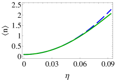
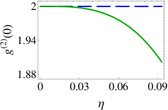
Figure 2: (a) The steady-state mean cavity photon number $\langle n\rangle\equiv\langle\bar{b}^{\dagger}\bar{b}\rangle$ as well as (b) its second-order correlation function $g^{(2)}(0)$ as a function of $\eta=g/(2\Omega)$. The blue long-dashed lines are plotted for single-photon processes, N=1, while the solid green ones for two-photon processes, N=2, respectively. Here, $\bar{n}=10^{-1}$, $\kappa/\gamma=10^{-3}$ and $\xi=0$.

In order to solve the infinite system of equations for $P_{n}$ (see e.g. Eq. 10 for two-photon processes), we truncate it at a certain maximum value $n=n_{max}$ so that a further increase of its value, i.e. $n_{max}$, does not modify the obtained results if other involved parameters are being fixed. Thus, generally the resonator’s steady-state mean quanta number can be expressed as:

$$\langle\bar{b}^{\dagger}\bar{b}\rangle=\sum^{n_{max}}_{n=0}nP_{n},$$ (11)

with

$$\sum^{n_{max}}_{n=0}P_{n}=1.$$ (12)

Respectively, the second-order photon-photon correlation function is defined in the usual way szu ; glauber , namely,

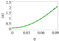
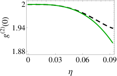
Figure 3: (a) The steady-state mean cavity photon number $\langle n\rangle\equiv\langle\bar{b}^{\dagger}\bar{b}\rangle$ as well as (b) its second-order correlation function $g^{(2)}(0)$ as a function of $\eta=g/(2\Omega)$. The solid green curves are plotted for two-photon processes, N=2, while the short-dashed black ones for three-photon processes, N=3, respectively. Other parameters are as in Fig. (2).

$$g^{(2)}(0) = \frac{\langle\bar{b}^{\dagger 2}\bar{b}^{2}\rangle}{\langle\bar{b}^{\dagger}\bar{b}\rangle^{2}}$$ (13)

$$= \bigl{(}1/\langle\bar{b}^{\dagger}\bar{b}\rangle^{2}\bigr{)}\sum^{n_{max}}_{n=0}n(n-1)P_{n}.$$

Note here that we need to evaluate the cavity field correlators, i.e. $\langle b^{\dagger}b\rangle$ etc., using Eq. (6) first. That is, one expresses $\langle b^{\dagger}b\rangle$ via $\langle\bar{b}^{\dagger}\bar{b}\rangle$ and calculate the latter correlator using the above developed approach. From Eq. (6) and within the performed approximations, one can observe however, that $\langle b^{\dagger}b\rangle$=$\langle\bar{b}^{\dagger}\bar{b}\rangle$ + $o(\eta^{4})$. Therefore, for $\eta\ll 1$, as it is the case considered here, we have $\langle b^{\dagger}b\rangle\approx\langle\bar{b}^{\dagger}\bar{b}\rangle$, and one can surely use the field operators $\{\bar{b},\bar{b}^{\dagger}\}$ to calculate the cavity mean-photon number and its second-order photon-photon correlations via expressions (11-13).

Thus, Figure (2) shows the steady-state mean photon numbers and their second-order photon-photon correlation functions for single-photon and two-photon processes plotted with the help of Eq. (8) and Eq. (10). One can observe here that these quantities differ from each other for single- and two-photon effects, respectively. For the sake of comparison, Figure (3) depicts similar things for two- and three-photon effects, correspondingly. Here, it is easy to see that the mean-photon numbers almost overlap for the two cases considered, whereas their second-order correlation functions distinguish from each other. One can proceed in the same vein with higher order photon processes. However, for identically considered parameters, their probabilities are small and the mean photon numbers are basically the same as indicated in Fig. 3(a). On the other side, the photon statistics exhibits quasi-thermal features as $\eta$ increases with other parameters being fixed. Concluding this part, more probable are processes with single-, two- and three-photons, respectively, if other involved parameters are being fixed, whereas the final cavity steady state is a quantum incoherent superposition of all those photons. Importantly, values different from $2$ for $g^{(2)}(0)$, occurring naturally for higher values of $\eta^{\prime}s$ with $\eta<1$, ensure the creation of this final cavity state which differs from a usual thermal state. Note that generally the environmental thermal mean-photon number will add linearly to the final photon flux (see, e.g., Eq. 9 for single-photon processes) so that an increase in the environmental temperature will lead to more output photons for the considered parameter ranges.

Figure 4: The cavity photon distribution function $P_{n}$ in the steady state. The green thin curve is plotted for $\eta=0.09$, while the thick blue one for $\eta=0.07$, respectively. Other parameters are as in Fig. (2).

Additionally, Figure (4) shows the photon distribution function $P_{n}=\langle n|\bar{\rho}|n\rangle$ for the same parameters as taken in Figs. (2) and (3), however, for five-photon processes, i.e. $N=5$. One can observe here that larger ratios of $\eta=g/(2\Omega)$, with $\eta<1$, lead to population of higher photon states, compare the thin green and thick blue curves plotted for $\eta=0.09$ and $\eta=0.07$, respectively, facilitating the generation of multiphoton states when $\kappa/\gamma\ll 1$. Correspondingly, $P_{n}$ is small for larger $n$ and smaller $\eta$, while $\eta<1$, assuring convergence of the results based on Eq. (7). One can observe that the probability of a two-photon state, that is $n=2$, is almost the same for $\eta=0.07$ and $\eta=0.09$, respectively, and it is higher than $0.1$. Thus a multiphoton superposition state around $n=2$ is generated when other parameters are being fixed. Furthermore, the same results, shown in the above figures will persist for moderate detunings, i.e., would not change significantly if $\xi\ll 1$.

Concluding here, the presence of diagonal dipole moments, in a resonance coherently pumped two-level system, makes possible the coupling to the resonator mode at a completely different frequency than the input one which drives the two-state quantum emitter, and cavity multiphoton state generation, respectively. Furthermore, the developed approach applies equally to a driven two-level quantum dot embedded in an acoustical phonon cavity see, e.g. nori ; knor ; cm ; erem . It can be generalized as well to an ensemble of two-level emitters agar having permanent dipoles and embedded in a microwave resonator. Finally notice that the results shown in Figs. (2-4) can be obtained directly by a full simulation of the master equation (1). However, in this case, one can not extract information about incoherent multiphoton processes that originate the final cavity steady state.

IV Summary

We have investigated the possibility to convert photons from, e.g. optical to microwave domains, via a resonantly pumped asymmetrical two-level quantum emitter embedded in a quantized single-mode resonator. The corresponding damping effects due to emitter’s spontaneous emission and cavity’s photon leakage are taking into account as well. The transition frequency of the two-level system differs significantly from the cavity’s one, namely, it can lay in the optical range while the resonator’s frequency in the microwave domain, respectively. Therefore, the two-state quantum emitter couples to the cavity mode through its diagonal dipole moments. As well, the cavity’s frequency is considering being far off-resonance from the generalized Rabi frequency resulting from the coherent driving of the two-level system via its non-diagonal dipole. In these circumstances, multiphoton absorption-emission processes are proper to the cavity quantum dynamics. We have demonstrated the cavity’s multiphoton characteristics and showed the feasibility for a certain output multiphoton superposition state generation. The photon statistics exhibits quasi-thermal photon statistics as the pumping parameter $\eta$ is increased from zero. Actually, values different from $2$ for the second-order photon-photon correlation function $g^{(2)}(0)$ ensure the creation of the cavity multiphoton superposition state. Finally, as a concrete system, where the approach developed here can apply, can serve asymmetrical two-level quantum dots coupled to microwave resonators as well as polar biomolecules, spin or quantum circuit systems, respectively twoa ; mqd1 ; mqd2 ; kov ; alt1 ; alt2 ; alt3 ; alt4 . In principle, coupling to terahertz or even higher-frequency resonators will allow photon conversion in these photon ranges too. As well, this analytical approach can be used to study non-resonant multiphonon quantum dynamics when a pumped two-level quantum dot interacts with an acoustical phonon resonator, respectively nori ; knor ; cm ; erem . Finally, it can be generalized to an ensemble of two-level emitters agar having permanent dipoles.

Appendix A The system’s Hamiltonian

Here we present details on how one arrives at the system’s Hamiltonian given by Eq. (2). The complete Hamiltonian describing the interaction of a two-level emitter possessing permanent dipoles with an external resonant coherent field as well as with a single-mode resonator, in the dipole and rotating wave approximations, is:

$$H = \hbar\omega b^{\dagger}b+\hbar\omega_{21}S_{z}-\hbar\Omega\bigl{(}S^{+}e^{-i\omega_{L}t}+S^{-}e^{i\omega_{L}t}\bigr{)}$$ (14)

$$+ \hbar g_{0}\bigl{(}d_{22}S_{22}+d_{11}S_{11}\bigr{)}\bigl{(}b^{\dagger}+b\bigr{)}+\hbar\bar{g}_{0}\bigl{(}S^{+}+S^{-}\bigr{)}$$

$$\times \bigl{(}b^{\dagger}+b\bigr{)}-E_{L}\bigl{(}d_{22}S_{22}+d_{11}S_{11}\bigr{)}\cos(\omega_{L}t).$$

Here the first two terms describe the free energies of the resonator and the two-level subsystem. The third and the sixth terms account for the interaction of the external laser field with the two-level emitter through its off-diagonal dipole moments $d_{21}$, $d_{21}=d_{12}$, as well as the diagonal dipole moments $d_{22}$ and $d_{11}$, respectively. Correspondingly, the fourth and the fifth components describe the interactions of the cavity mode with the two-level emitter via diagonal and off-diagonal dipole moments. Here, $E_{L}$ is the amplitude of the external driving field, while $g_{0}=\sqrt{2\pi\omega/\hbar V}$ where $V$ is the quantization volume, and $\bar{g}_{0}=g_{0}d_{21}$. $S_{\alpha\alpha}$, $\{\alpha=1,2\}$, are the population operators, respectively. All other parameters and operators are described in Section II.

After performing a unitary transformation $\bar{U}(t)=\exp{(i\omega_{L}S_{z}t)}$ one can observe that the fifth Hamiltonian’s term is a rapidly oscillating one since $\omega_{L}$ is bigger than the corresponding coupling strength, i.e., $\omega_{L}\gg\bar{g}_{0}$ and $\omega_{L}\gg\omega$. As well, the last component of the Hamiltonian (14) can be neglected from the same reason because $\omega_{L}\gg\{E_{L}d_{22}/\hbar,E_{L}d_{11}/\hbar\}$ for moderate assumed external pumping strengths. Thus, one has then the following Hamiltonian

$$H = \hbar\omega b^{\dagger}b+\hbar\Delta S_{z}-\hbar\Omega\bigl{(}S^{+}+S^{-}\bigr{)}+\hbar gS_{z}\bigl{(}b^{\dagger}+b\bigr{)}$$ (15)

$$+ \hbar g_{0}(d_{11}+d_{22})(b^{\dagger}+b\bigr{)}/2,$$

where $g=g_{0}(d_{22}-d_{11})$, and we have used also the relations $S_{22}=1/2+S_{z}$, and $S_{11}=1/2-S_{z}$. Further, performing a unitary transformation $V=\exp{(\zeta b-\zeta^{\ast}b^{\dagger})}$, with $\zeta=g_{0}(d_{11}+d_{22})/[2(\omega+i\kappa/2)]$, in the whole master equation (1), containing the Hamiltonian (15), one arrives at the same form of the master equation with, however, the Hamiltonian (2), and where $\Delta\equiv\Delta-g^{2}_{0}(d^{2}_{22}-d^{2}_{11})/\omega$, when $\omega\gg\kappa$. The last term from the detuning’s expression can be used to redefine the emitter’s frequency, i.e., $\omega_{21}\equiv\omega_{21}-g^{2}_{0}(d^{2}_{22}-d^{2}_{11})/\omega$, so one finally has $\Delta=\omega_{21}-\omega_{L}$.

Now, if we make a unitary transformation in the Hamiltonian (2), $\bar{V}(t)=\exp{(i\omega b^{\dagger}bt)}$, then it transforms as:

$$H=\hbar\Delta S_{z}-\hbar\Omega\bigl{(}S^{+}+S^{-}\bigr{)}+\hbar gS_{z}\bigl{(}b^{\dagger}e^{i\omega t}+be^{-i\omega t}\bigr{)}.$$

(16)

If one avoids any resonances in the system with respect to the resonator’s frequency or its multiples, as it is the case here, then the last term in the above Hamiltonian is a rapidly oscillating one, if $\omega$ is significantly larger than $g$, and may be neglected. Section II develops an approach where the contribution of this term is perturbatively calculated for moderately intense externally applied fields and appropriate parameters ranges, i.e. $\omega>2\Omega\gg\{g,\gamma,\kappa\}$, respectively.

Appendix B The master equation (7) containing terms up to $\eta^{4}$

Here, we shall emphasize some processes occurring in our setup in more details, namely, the single- and two-photon effects. Let’s write down the time-independent damping part of the master equation (7), taking into account expansion terms up to $\eta^{4}$, namely,

$$\frac{d}{dt}\bar{\rho} = -\frac{\gamma\eta^{2}}{8(1+\xi^{2})^{2}}\biggl{\{}\bigl{[}\bar{b},\bar{b}^{\dagger}\bar{\rho}\bigr{]}+\bigl{[}\bar{b}^{\dagger},\bar{b}\bar{\rho}\bigr{]}\biggr{\}}-\frac{\gamma\eta^{4}(1+4\xi^{2})}{32(1+\xi^{2})^{4}}\biggl{\{}\bigl{[}(\bar{b}\bar{b}^{\dagger}+\bar{b}^{\dagger}\bar{b}),(\bar{b}\bar{b}^{\dagger}+\bar{b}^{\dagger}\bar{b})\bar{\rho}\bigr{]}+\bigl{[}\bar{b}^{2},\bar{b}^{\dagger 2}\bar{\rho}\bigr{]}+\bigl{[}\bar{b}^{\dagger 2},\bar{b}^{2}\bar{\rho}\bigr{]}\biggr{\}}$$ (17)

$$+ \frac{3\gamma\eta^{4}(1-2\xi^{2})}{8(1+\xi^{2})^{4}}\biggl{\{}\bigl{[}\bar{b}^{\dagger}(1+\bar{b}^{\dagger}\bar{b}),\bar{b}\bar{\rho}\bigr{]}+\bigl{[}(1+\bar{b}^{\dagger}\bar{b})\bar{b},\bar{b}^{\dagger}\bar{\rho}\bigr{]}\biggr{\}}-\frac{\kappa}{2}(1+\bar{n})\bigl{[}\bar{b}^{\dagger},\bar{b}\bar{\rho}\bigr{]}-\frac{\kappa}{2}\bar{n}\bigl{[}\bar{b},\bar{b}^{\dagger}\bar{\rho}\bigr{]}+H.c.,$$

where smaller contributions, proportional to $\kappa\eta^{4}$, were neglected since we have considered that $\kappa/\gamma\ll 1$.

One can observe that terms proportional to $\eta^{2}$ describe single-photon processes, that is, the photon number in the distribution function $P_{n}$ ($P_{n}=\langle n|\bar{\rho}|n\rangle$ with $n\in\{0,1,2,\cdots\}$) will change by $\pm 1$, i.e. $P_{n\pm 1}$, see also Eq. (8). Respectively, the terms proportional to $\eta^{4}$ account for two-photon effects. For instance, the last two commutators from the second term of Eq. (17) will modify the photon number in the distribution function $P_{n}$ by $\pm 2$, i.e. $P_{n\pm 2}$, see also Eq. (10) and Fig. (1). Concluding this part, one can generalize that terms proportional to $\eta^{2N}$, in the master equation (7), account for $N$-photon processes, respectively.

From Eq. (17) one can easily arrive at Eq. (10). Setting then $\eta^{4}\to 0$, we obtain the Eq. (8). The steady-state solution of Eq. (8), accounting for single-photon processes only, can be expressed as:

$$P_{n}=Z^{-1}e^{-\alpha n},$$ (18)

where the normalization $Z$ is determined by the requirement $\sum^{\infty}_{n=0}P_{n}=1$, that is $Z=\sum^{\infty}_{n=0}e^{-\alpha n}$, whereas $\alpha={\rm ln}\beta$ and $\beta=\kappa_{1}/\kappa_{2}$ with $\kappa_{1}=\kappa(1+\bar{n})$+$\gamma\eta^{2}/[4(1+\xi^{2})^{2}]$, and $\kappa_{2}=\kappa\bar{n}$+$\gamma\eta^{2}/[4(1+\xi^{2})^{2}]$. The mean-photon number is determined via

$$\langle\bar{b}^{\dagger}\bar{b}\rangle=\sum^{\infty}_{n=0}nP_{n}=\frac{1}{\beta-1}=\bar{n}+\frac{\gamma\eta^{2}}{4\kappa(1+\xi^{2})^{2}},$$ (19)

which is exactly the expression (9). We finalize by noting that, unfortunately, finding the analytic solution of Eq. (17) or Eq. (10), incorporating both single- and two-photon processes, is not a trivial task.

References

- (1) H. J. Kimble, The quantum internet, Nature (London) 453, 1023 (2008).
- (2) Y.-P. Huang, V. Velev, and P. Kumar, Quantum frequency conversion in nonlinear microcavities, Opt. Lett. 38, 2119 (2013).
- (3) T. E. Northup, and R. Blatt, Quantum information transfer using photons, Nat. Photonics 8, 356 (2014).
- (4) D. P. Lake, M. Mitchell, B. C. Sanders, and P. E. Barclay, Two-colour interferometry and switching through optomechanical dark mode excitation, Nat. Communications 11:2208, 1 (2020).
- (5) J. Huang, and P. Kumar, Observation of Quantum Frequency Conversion, Phys. Rev. Lett. 68, 2153 (1992).
- (6) M. T. Rakher, L. Ma, O. Slattery, X. Tang, and K. Srinivasan, Quantum transduction of telecommunications-band single photons from a quantum dot by frequency upconversion, Nat. Photonics 4, 786 (2010).
- (7) X. Guo, C.-L. Zou, H. Jung, and H. X. Tang, On-Chip Strong Coupling and Efficient Frequency Conversion between Telecom and Visible Optical Modes, Phys. Rev. Lett. 117, 123902 (2016).
- (8) J. Han, Th. Vogt, Ch. Gross, D. Jaksch, M. Kiffner, and W. Li, Coherent Microwave-to-Optical Conversion via Six-Wave Mixing in Rydberg Atoms, Phys. Rev. Lett. 120, 093201 (2018).
- (9) O. V. Kibis, G. Ya. Slepyan, S. A. Maksimenko, and A. Hoffmann, Matter Coupling to Strong Electromagnetic Fields in Two-Level Quantum Systems with Broken Inversion Symmetry, Phys. Rev. Lett. 102, 023601 (2009).
- (10) F. Oster, C. H. Keitel, and M. Macovei, Generation of correlated photon pairs in different frequency ranges, Phys. Rev. A 85, 063814 (2012).
- (11) A. F. Kockum, V. Macri, L. Garziano, S. Savasta, and F. Nori, Frequency conversion in ultrastrong cavity QED, Scientific Reports 7: 5313, 1 (2017).
- (12) M. D’Angelo, M. V. Chekhova, and Y. Shih, Two-Photon Diffraction and Quantum Lithography, Phys. Rev. Lett. 87, 013602 (2001).
- (13) C. Sanchez Munoz, E. del Valle, A. Gonzalez Tudela, K. Müller, S. Lichtmannecker, M. Kaniber, C. Tejedor, J. J. Finley, and F. P. Laussy, Emitters of N-photon bundles, Nature Photonics 8, 550 (2014).
- (14) D. L. Andrews, D. S. Bradshaw, K. A. Forbes, and A. Salam, Quantum electrodynamics in modern optics and photonics: tutorial, Jr. Opt. Soc. Am. B 37, 1153 (2020).
- (15) C. J. Villas-Boas, and D. Z. Rossatto, Multiphoton Jaynes-Cummings Model: Arbitrary Rotations in Fock Space and Quantum Filters, Phys. Rev. Lett. 122, 123604 (2019).
- (16) S. V. Vintskevich, D. A. Grigoriev, N. I. Miklin, and M. V. Fedorov, Entanglement of multiphoton two-mode polarization Fock states and of their superpositions, Laser Phys. Lett. 17, 035209 (2020).
- (17) W.-T. Liao, and A. Palffy, Optomechanically induced transparency of x-rays via optical control, Scientific Reports 7:321, 1 (2017).
- (18) Q. Bin, X.-Y. Lü, F. P. Laussy, F. Nori, and Y. Wu, N-Phonon Bundle Emission via the Stokes Process, Phys. Rev. Lett. 124, 053601 (2020).
- (19) L. Garziano, V. Macri, R. Stassi, O. Di Stefano, F. Nori, and S. Savasta, One Photon Can Simultaneously Excite Two or More Atoms, Phys. Rev. Lett. 117, 043601 (2016).
- (20) I. Yu. Chestnov, V. A. Shakhnazaryan, I. A. Shelykh, and A. P. Alodjants, Ensemble of Asymmetric Quantum Dots in a Cavity As a Terahertz Laser Source, JETP Lett. 104, 169 (2016).
- (21) I. Yu. Chestnov, V. A. Shahnazaryan, A. P. Alodjants, and I. A. Shelykh, Terahertz Lasing in Ensemble of Asymmetric Quantum Dots, ACS Photonics 4, 2726 (2017).
- (22) V. A. Kovarskii, and O. B. Prepelitsa, Effect of a polar environment on the resonant generation of higher optical harmonics by dipole molecules, Optics and Spectroscopy 90, 351 (2001).
- (23) M. A. Anton, S. Maede-Razavi, F. Carreno, I. Thanopulos, and E. Paspalakis, Optical and microwave control of resonance fluorescence and squeezing spectra in a polar molecule, Phys. Rev. A 96, 063812 (2017).
- (24) P. Kirton, and J. Keeling, Nonequilibrium Model of Photon Condensation, Phys. Rev. Lett. 111, 100404 (2013).
- (25) Ya. S. Greenberg, Low-frequency Rabi spectroscopy of dissipative two-level systems: Dressed-state approach, Phys. Rev. B 76, 104520 (2007).
- (26) F. Yoshihara, T. Fuse, S. Ashhab, K. Kakuyanagi, Sh. Saito, and K. Semba, Superconducting qubit–oscillator circuit beyond the ultrastrong-coupling regime, Nature Physics 13, 44 (2017).
- (27) G.-W. Deng, D. Wei, S.-X. Li, J. R. Johansson, W.-Ch. Kong, H.-O. Li, G. Cao, M. Xiao, G.-C. Guo, F. Nori, H.-W. Jiang, and G.-P. Guo, Coupling two distant double quantum dots with a microwave resonator, Nano Lett. 15, 6620 (2015).
- (28) M. C. Arnesen, S. Bose, and V. Vedral, Natural Thermal and Magnetic Entanglement in the 1D Heisenberg Model, Phys. Rev. Lett. 87, 017901 (2001).
- (29) D. Braun, Creation of Entanglement by Interaction with a Common Heat Bath, Phys. Rev. Lett. 89, 277901 (2002).
- (30) A. M. Basharov, Entanglement of atomic states upon collective radiative decay, JETP Lett. 75, 123 (2002).
- (31) Z. Ficek, and R. Tanas, Entangled states and collective nonclassical effects in two-atom systems, Phys. Rep. 372, 369 (2002).
- (32) A. Hewgill, A. Ferraro, and G. De Chiara, Quantum correlations and thermodynamic performances of two-qubit engines with local and common baths, Phys. Rev. A 98, 042102 (2018).
- (33) G. S. Agarwal, Quantum Statistical Theories of Spontaneous Emission and their Relation to other Approaches (Springer, Berlin, 1974).
- (34) M. O. Scully, and M. S. Zubairy, Quantum Optics (Cambridge University Press, Cambridge, 1997).
- (35) J. Peng, and G.-x. Li, Introduction to Modern Quantum Optics (World Scientific, Singapore, 1998).
- (36) N. A. Enaki, Collective resonance fluorescence of extended two-level media, Optics and Spectroscopy 66, 629 (1989).
- (37) A. P. Saiko, S. A. Markevich, and R. Fedaruk, Multiphoton Raman transitions and Rabi oscillations in driven spin systems, Phys. Rev. A 98, 043814 (2018).
- (38) M. Macovei, J. Evers, and C. H. Keitel, Spontaneous decay processes in a classical strong low-frequency laser field, Phys. Rev. A 102, 013718 (2020).
- (39) This formula can be derived by taken various values for , or alternatively for any , see for instance the following link: https://mathoverflow.net/questions/78813/binomial-expansion-for-non-commutative-setting.
- (40) R. J. Glauber, The Quantum Theory of Optical Coherence, Phys. Rev. 130, 2529 (1963).
- (41) J. Kabuss, A. Carmele, T. Brandes, and A. Knorr, Optically Driven Quantum Dots as Source of Coherent Cavity Phonons: A Proposal for a Phonon Laser Scheme, Phys. Rev. Lett. 109, 054301 (2012).
- (42) V. Ceban, and M. A. Macovei, Sub-Poissonian phonon statistics in an acoustical resonator coupled to a pumped two-level emitter, JETP 121, 793 (2015).
- (43) V. Eremeev, and M. Orszag, Phonon maser stimulated by spin postselection, Phys. Rev. A 101, 063815 (2020).