Improving information retrieval from electronic health records using dynamic and multi-collaborative filtering
Ziwei Fan1, Evan Burgun2, Zhiyun Ren3, Titus Schleyer4,5, Xia Ning3,6*
1 Department of Computer Science, University of Illinois at Chicago, Chicago, USA
2 CSCI Consulting Inc., Indianapolis, IN, USA
3 Department of Biomedical Informatics, The Ohio State University, Columbus, OH, USA
4 Regenstrief Institute, Indianapolis, IN, USA
5 Indiana University School of Medicine, Indianapolis, IN, USA
6 Department of Computer Science and Engineering, The Ohio State University, Columbus, OH, USA
* ning.104@osu.edu
Abstract
Due to the rapid growth of information available about individual patients, most physicians suffer from information overload when they review patient information in health information technology systems. In this manuscript, we present a novel hybrid dynamic and multi-collaborative filtering method to improve information retrieval from electronic health records. This method recommends relevant information from electronic health records for physicians during patient visits. It models information search dynamics using a Markov model. It also leverages the key idea of collaborative filtering, originating from Recommender Systems, to prioritize information based on various similarities among physicians, patients and information items. We tested this new method using real electronic health record data from the Indiana Network for Patient Care. Our experimental results demonstrated that for 46.7% of testing cases, this new method is able to correctly prioritize relevant information among top-5 recommendations that physicians are truly interested in.
Introduction
When we consider buying a book on Amazon’s Website, we often benefit from items listed in a section called “Recommended for you.” These recommendations, generated by a method called Collaborative Filtering () [1], suggest items of possible interest based on what other customers have viewed and purchased. Often, these suggestions are very useful and lead to additional purchases. However, when physicians search the electronic health records (EHRs) with regard to a particular patient problem, the EHRs do not make suggestions for potentially useful information. Instead, it requires physicians to go through the same manual, cumbersome and laborious process of searching for and retrieving information for similar patients/problems every single time.
In this manuscript, we present , a novel hybrid Dynamic and multi-Collaborative Filtering method, for information recommendation when physicians search for information from patient EHRs. integrates the following two key ideas:
-
•
collaborative filtering, which prioritizes information items based on what similar physicians have searched for on similar patients; and
-
•
dynamic modeling, which foresees future information items of interest based on how physicians search for information items over time.
Here, dynamics refers to the information retrieval patterns over time (e.g., in which order different information items are searched for; which information item will be typically searched for after a certain information item has been retrieved). Multi-collaborative filtering () refers to that multiple types of similarities (e.g., physician similarities, patient similarities and information similarities) are integrated to score information items of possible interest. models information retrieval dynamics by a first-order Markov Chain (), and combines transition probabilities (discussed in Section Markov Chain-based Scoring) with scores to produce final recommendation scores for future interested information items. recommends the information items with the highest scores to physicians. We tested on a real dataset from the Indiana Network for Patient Care (INPC). Our experimental results demonstrate 22.3% improvement from over models on top-1 recommendation (i.e., only the top recommended information item is considered), and for 46.7% of all the testing cases, is able to correctly identify information items that are truly interested by physicians among its top-5 recommendations.
Literature Review
The most relevant research to our work is from Recommender Systems, a research area that originated in computer science. In particular, top- recommender systems, which recommend the top- items that are most likely to be preferred or purchased by users, have been used in a variety of applications in e-commerce. The top- recommendation methods can be broadly classified into two categories [1]. The first category is neighborhood-based collaborative filtering methods [2], which leverage information from similar users and/or similar items to generate recommendations. The second category is model-based methods, particularly latent factor models which learn user and item latent factors and determine user preference over items using the factors. Recent recommendation methods also include deep learning based approaches [3], in which user preferences, item characteristics and user-item interactions can be learned in deep architectures.
Dynamic recommender systems have been developed to recommend information of interest over time. Popular techniques include latent factor transition approaches [4], and Markov models [5] that model the transitions among latent factors capturing information preference; state space approaches [6, 7] that model the transitions across different states over time; point processes [8] and other statistical models [9] that learn probabilities of future events.
Recommendation methods have been recently used to recommend and prioritize healthcare information, due to the rapid growth of information available about individual patients and the tremendous need for personalized healthcare [10]. Current applications of recommender systems in healthcare include recommending physicians to patients on specific diseases [11, 12]; recommending drugs [13], medicine [14] and therapies [15]; and recommending nursing care plans [16], etc.
Terminologies, Definitions and Notations
| notation | description |
|---|---|
| /// | a physician/patient/term/visit |
| a search term sequence of on in visit | |
| a set of physicians similar to | |
| a set of patients similar to | |
| a set of terms similar to |
In EHR systems, there is no measurement similar to numerical rating values in Amazon that can be used to quantitatively assess how much a physician is interested in a certain information item. In this case, we take a type of implicit feedback as a qualitative measurement. That is, if a physician searches for an information item from a patient’s EHR data, the physician is considered as interested in that information item during the diagnostic process of the patient, and that information item is useful for/relevant to the diagnosis of the patient. Thus, to evaluate whether a physician is interested in an information item on a patient, we can check whether the physician searches for the information item from the patient’s EHR data. Since search is typically done through submitting a search term, we use the two terms “search term” and “information item” exchangeably, and the problem becomes to recommend the next search term that a physician is interested in on a certain patient.
In this manuscript, a physician is denoted as , a patient is denoted as , and a search term is denoted as . A sequence of search terms that a physician searches for on a certain patient during a certain patient visit is represented as
| (1) |
where is the -th search term during visit . Note that a physician may have multiple search sequences on a same patient during different visits. The physician who we recommend a next search term to on a patient is referred to as the target physician, and the corresponding patient is referred to as the target patient. A set of physicians/patients similar to the target physician /target patient is denoted as /, respectively. A set of search terms similar to a particular search term is denoted as . The size of a set is denoted as . Additional notations will be introduced when they are used (e.g., in Section Similarity Calculation). Table 1 presents the important notations that we use in this manuscript.
Overview of the Dynamic and Multi-Collaborative Filtering Method –
In this manuscript, we tackle the problem of recommending the next search term to a physician while the physician is searching for information about a patient. The key idea is to analyze search patterns in order to make recommendations for potentially useful, other information to the physician. To do so, we score and prioritize possible recommendations based on the following two criteria combinatorially:
-
•
which terms the physician has searched for on the patient already and
-
•
which terms similar physicians have searched for on similar patients.
The first criterion considers the search dynamics under the assumption that the past behavior of physicians is a reasonable approximation for the standard of care [17, 18], and their future behavior follows a same standard of care. Thus, future search terms can be inferred from previously searched terms and their orders. The second criterion considers patient similarities and physician similarities. The underlying intuition is that patients share commonalities and similar patients stimulate similar information retrieval patterns by physicians. Likewise, physicians share commonalities which result in similar search patterns on patients.
We propose the hybrid method that considers search dynamics and multiple similarities for the next search term recommendation. consists two scoring components. The first component is designed to address search dynamics through a first-order Markov Chain [19]. The score of a possible search term from this dynamics-based scoring component is denoted as . The second component is to score search terms based on similarities via multi-collaborative filtering. The score of a possible search term from this similarity-based scoring component is denoted as . Thus, scores a next possible search term for a physician on a patient after a sequence of searches (Equation 1) as a linear combination of and , that is,
| (2) |
where is a weighting parameter.
In this manuscript, if a score is generated from a certain method , a superscript X will be included on the score notation (e.g., , or ). In general, a superscript X indicates an associated method . All possible terms are first scored using the scoring function in Equation 2. The top-scored terms are recommended as the next possible search terms. The first-order Markov Chain-based scoring and the multi-collaborative filtering-based scoring will be discussed in Section Markov Chain-based Scoring and Section Multi-Collaborative Filtering-based Scoring, respectively. Table 2 lists all the methods in the manuscript.
| notation | method description |
|---|---|
| dynamic and multi-collaborative filtering method (Section Overview of the Dynamic and Multi-Collaborative Filtering Method – ) | |
| first-order markov chain-based scoring method (Section First-Order Markov Chain-based Scoring – ) | |
| physician-patient-similarity-based scoring method (Section Physician-Patient-Similarity-based CF Scoring – ) | |
| transition-involved patient-term-similarity-based scoring method (Section Transition-Involved Patient-Term-Similarity-based CF Scoring – ) | |
| patient-first similarity identification (Section Identifying similar physicians and similar patients) | |
| physician-first similarity identification (Section Identifying similar physicians and similar patients) |
Markov Chain-based Scoring
Background on Markov Chains
Markov Chain () [19] represents a very fundamental dynamic modeling scheme based on the Markovian assumption. The Markovian assumption states that in a sequence of events , each event is only dependent on a small set of previous consecutive events but independent of any earlier events. An models a sequence of events so that each of the events follows the Markovian assumption. The Markovian assumption is statistically represented as , where is the probability of observing event given the previous event sequence . The number of previous events that depends on (i.e., in ) defines the order of the . A special is first-order , in which each event only depends on its immediate precursor. has been demonstrated to be very effective in modeling, approximating and analyzing real-life sequence data [19].
First-Order Markov Chain-based Scoring –
We use a first-order as the dynamic model to simulate the sequence of terms that a physician searches for on a patient during a visit. This method is referred to as first-order Markov Chain, denoted as . For a sequence , calculates a dynamics-based score of a next possible search term after as the transition probability from to , that is,
| (3) |
where is the transition probability from to in a first-order . The transition probability from a term to another term in a first-order is calculated as the ratio of the total frequency of transitions from to over the total frequency of all transitions from to any terms, that is,
| (4) |
where represents that is in , is the frequency of the transitions from to in . Thus, as in Equation 3 is not specific to a particular physician or patient, but corresponds to clinical practices that are summarized from all available physicians and patients.
Multi-Collaborative Filtering-based Scoring
Background on Collaborative Filtering
Collaborative Filtering () is a popular technique in Recommender Systems [1] for recommending items to a target user. The fundamental idea of is that “similar users like similar items”. User-based methods first identify similar users to the target user, and then recommend to the target user the items that are preferred by similar users. Item-based methods first identify items similar to the target user’s preferred items, and then recommend to the target user such similar items. Thus, methods heavily depend on the calculation of user similarity and item similarity. A typical way to calculate user similarity is to represent each user using her preference profile over items, and calculate user similarity as the item preference profile similarity. Likewise, a typical way to calculate item similarity is to represent each item using its preference profiles across users, and calculate item similarity as the user preference profile similarity. The user similarity function and item similarity function in are often pre-defined, and thus the recommendations based on similarities can be easily interpreted. is particularly powerful when user and item data are sparse, which is often the case in real-life applications. is also well-known for its scalability on large-scale problems, particularly when the user similarity and item similarity can be calculated in parallel trivially.
Physician-Patient-Similarity-based CF Scoring –
We developed a method that generates search term recommendations from similar physicians and patients. This method first identifies similar physicians and similar patients (discussed in Section Identifying similar physicians and similar patients) and then scores terms searched by similar physicians on similar patients (discussed in Section Collaborative Filtering in ). This method is referred to as physician-patient-similarity-based Collaborative Filtering, and denoted as .
Identifying similar physicians and similar patients
We developed two approaches to identifying the set of similar physicians and the set of similar patients, depending on which set is identified first.
Patient-First Similarity Identification – In the first approach, a set of patients similar to the target patient is first identified, and then based on the similar patients, a set of physicians similar to the target physician is then selected. This approach is denoted as (i.e., from Patients to phYsicians). In , the set of patients similar to the target patient is represented as
| (5) |
and is composed of the top- most similar patients to the target patient (patient-patient similarity will be discussed later in Section Similarity Calculation). Given , a set of physicians similar to the target physician is represented as
| (6) |
and selected as follows: first, physicians who have ever searched for same terms on and on one or more patients in are identified. From such physicians, the top- most similar physicians to are selected into (physician-physician similarity will be discussed later in Section Similarity Calculation).
Physician-First Similarity Identification – The second approach is to first identify a set of physicians similar to the target physician , and then based on the similar physicians, to identify a set of similar patients. This approach is denoted as (i.e., from phYsicians to Patients). In , the set of similar physicians is represented as
| (7) |
and has the top- most similar physicians to . Based on , a set of patients similar to the target patient , denoted as
| (8) |
is identified as patient ’s top- most similar patients on whom physicians in have ever searched for same terms as on .
Collaborative Filtering in
From and (either and , or and ), a set of physician-patient-term triplets, denoted as , is constructed. That is, has all the triplets such that physician has searched for term for patient . Thus, for a sequence , the score of a next possible search term is calculated as follows:
| (9) | ||||
where and is the frequency of the triplet (i.e., how many times searches for on in total); is the average frequency of all possible terms that searches for on ; is the centered frequency for (i.e., shifted by ) in order to reduce the bias from searches with different frequencies; and and are the similarity between and , and the similarity between and , respectively (discussed in Section Similarity Calculation). The intuition behind the scoring scheme in Equation 9 is that the possibility that searches for on after a sequence of searches is the aggregation of 1). the average possibility of searching for arbitrary search terms (i.e., the first term in Equation 9), and 2). the possibility that similar physicians search for on similar patients (i.e., the second term in Equation 9).
Transition-Involved Patient-Term-Similarity-based CF Scoring –
The order in which a physician searches for different terms could indicate a diagnosis process, and therefore the search order deserves additional consideration. We developed a new patient-term-similarity-based scoring method that involves the transitions among search terms. Patient similarities and term similarities are considered in this method, which is different from those in (i.e., physician similarities and patient similarities in ). This method is referred to as Transition-involved patient-term-similarity-based Collaborative Filtering, denoted as .
aggregates from all similar patients the transitions from the last search term in a sequence (Equation 1) to another search term. Specifically, identifies a set of patients similar to the target patient and a set of terms similar to the last search term in . The set contains the terms with term-term similarity (discussed in Section Similarity Calculation) to above a threshold . Then looks into what physicians search for on patients in after they searched for a similar term in . The underlying assumption is that similar patients stimulate similar patterns of search sequences. Thus, the score of a next possible search term is calculated as follows:
| (10) |
where is the frequency of transitions from term to term for patient from all possible searches on , is the term-term similarity between and (discussed in Section Similarity Calculation).
Similarity Calculation
Physician-Physician Similarities – We first represent each physician using a vector of search term frequencies, denoted as . Each dimension of corresponds to a term, and the value in each dimension of is the total frequency that the corresponding term has been searched by . Note that the frequency is aggregated from all the patients that searches on. This representation scheme is very similar to the bag-of-word representation in text mining [20]. Given the representation, the similarity between two physicians and is calculated as the cosine similarity between and , that is,
| (11) |
The intuition is that the search term distribution indicates physician specialties and expertise, and physicians of similar specialties and expertise are considered similar.
Patient-Patient Similarities – Similarly as for physicians, each patient is also represented using a vector of term frequencies, denoted as . Each dimension of corresponds to a term, and the value in each dimension of is the total frequency of the corresponding term searched for by all physicians. The term distribution represents the health histories of the patient, and thus a reasonable patient representation. Given the representation, the similarity between two patients and is calculated as the cosine similarity between and , that is,
| (12) |
Term-Term Similarities – Each term is represented using a vector of patient frequencies, denoted as . Each dimension in corresponds to a patient, and the value in each dimension of is the total frequency that term is searched for by all physicians. The term-term similarity between terms and is calculated as the cosine similarity between and , that is,
| (13) |
The underlying assumption is that if two terms are frequently searched for on a same patient, they are considered as similar in their medical meanings and relatedness.
Materials
Data
| dataset | # | # | # | # | len() | len()/# | len()/# |
|---|---|---|---|---|---|---|---|
| INCP | 13,819 | 2,121 | 9,781 | 24,183 | 69,770 | 5.049 | 2.885 |
| (training) | 8,471 | 1,542 | 6,550 | 13,677 | 38,553 | 4.551 | 2.819 |
| (testing) | 624 | 147 | 654 | 692 | 2,506 | 4.016 | 3.621 |
-
•
In this table, # is the number of patients; # is the number of physicians; # is the number of terms; # is the number of sequences; len() is total length of sequences; len()/# is average length of sequences per patient and len()/# is average length of sequences.
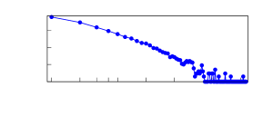
The data we use for experiments come from the Indiana Network for Patient Care (INPC) 111IRB Protocol # 1612682149 “Supporting information retrieval in the ED through collaborative filtering”.. The INPC is Indiana’s major health information exchange, and offers physicians access to the most complete, cross-facility virtual electronic patient records in the nation. Implemented in the 1990s, the INPC collects data from over 140 Indiana hospitals, laboratories, long-term care facilities and imaging centers. We extracted the INPC search logs that were generated between 01/24/2013 to 09/24/2013. Table 3 presents the statistics of the INPC dataset. Figure 1 presents the distribution of sequence length in the dataset. It is notable that search sequences are typically very short (on average 2.89 search terms per each sequence). Figure 2 presents the distribution of the number of unique terms for each patient. On average, each patient has 3.85 unique search terms. The short sequences and small number of unique search terms per patient make the recommendation problem difficult, because the available data are very sparse.
Experimental Protocols and Evaluation Metric
We use the following experimental protocol to evaluate our methods on the INPC dataset: all the search sequences are split by the same cut-off time. Any searches before the cut-off time are in the training set, and any searches after the cut-off time are in the testing set. The models are trained using only training set, for example, the transition probabilities (Equation 4) are constructed only using the search sequences and terms in training set, and the various similarities (Equation 11, 12 and 13) are calculated only from the training set. This protocol is referred to as cut-off cross validation, denoted as . Figure 3 demonstrates the experimental protocol.

We use the cut-off time 08/15/2013 (additional results for other cut-off times are available in the supplementary materials222https://cs.iupui.edu/~zifan/sub.pdf). This cut-off time is selected because sufficient search terms from a majority of the search sequences are retained in training set before the cut-off time and meanwhile sufficient search sequences have testing terms after the cut-off time. After the split, the statistics for the training and testing data is presented in Table 3 (in “” rows). This setting is close to the realistic scenario, that is, all the data before a certain time should be used to predict information after that time. However, a shortcoming of is that many early search sequences may not have testing terms, and many late search sequences will not have anything in the training set. Sequences that do not have testing terms are still used to train models. Sequences that do not have training terms are not used. For those sequences which have terms after the cut-off time, only the first one of the terms after the cut-off time will be used for evaluation.
The model performance is measured using Hit-Rate at (HR@). For a sequence, a hit is defined as a recommended term that is truly the next search term. HR@ is the percentage of testing sequences that have a hit and the hit appears among the top- recommended terms. Higher HR@ values indicate better performance.
Experimental Results and Discussions
Overall Performance
| method | sim | HR@1 | HR@2 | HR@3 | HR@4 | HR@5 | |||||
| - | - | - | - | - | 0.202 | 0.297 | 0.338 | 0.378 | 0.393 | ||
| - | - | 0.249 | 0.355 | 0.406 | 0.417 | 0.428 | |||||
| - | - | 0.215 | 0.336 | 0.393 | 0.424 | 0.441 | |||||
| - | - | 0.222 | 0.342 | 0.393 | 0.422 | 0.443 | |||||
| - | - | 0.262 | 0.292 | 0.305 | 0.310 | 0.320 | |||||
| - | - | 0.254 | 0.329 | 0.350 | 0.368 | 0.378 | |||||
| - | - | 0.237 | 0.312 | 0.357 | 0.372 | 0.381 | |||||
| - | - | 0.230 | 0.312 | 0.355 | 0.381 | 0.393 | |||||
| - | - | 0.211 | 0.273 | 0.336 | 0.374 | 0.398 | |||||
| - | - | - | 0.213 | 0.279 | 0.303 | 0.322 | 0.331 | ||||
| - | - | - | 0.189 | 0.290 | 0.320 | 0.340 | 0.355 | ||||
| - | - | - | 0.200 | 0.284 | 0.329 | 0.355 | 0.378 | ||||
| - | - | - | 0.200 | 0.282 | 0.327 | 0.357 | 0.379 | ||||
| - | - | 0.247 | 0.357 | 0.426 | 0.441 | 0.464 | |||||
| - | 0.245 | 0.363 | 0.422 | 0.439 | 0.464 | ||||||
| - | 0.226 | 0.351 | 0.404 | 0.430 | 0.467 | ||||||
| - | 0.254 | 0.329 | 0.353 | 0.379 | 0.426 | ||||||
| - | 0.230 | 0.346 | 0.366 | 0.402 | 0.432 | ||||||
| - | 0.230 | 0.331 | 0.391 | 0.424 | 0.447 | ||||||
| - | 0.222 | 0.331 | 0.383 | 0.430 | 0.447 | ||||||
| - | 0.222 | 0.323 | 0.378 | 0.426 | 0.449 | ||||||
| - | - | - | 0.228 | 0.307 | 0.335 | 0.359 | 0.379 | ||||
| - | - | 0.213 | 0.312 | 0.348 | 0.376 | 0.398 | |||||
| - | - | 0.213 | 0.303 | 0.353 | 0.376 | 0.400 | |||||
| - | - | 0.209 | 0.297 | 0.344 | 0.383 | 0.406 | |||||
| - | - | 0.200 | 0.310 | 0.346 | 0.381 | 0.413 |
-
•
In this table, the column “sim” corresponds to similarity identification methods; is the weight on CF component in ; is the number of similar patients; is the number of similar physicians; is the similarity threshold to identify similar terms. The best performance of each method under each metric is bold. The best overall performance of all methods under each metric is underlined.
We compare , , and , as well as their variations, in our experiments. Table 4 presents the best performance of each method. Overall, - with is the best method because 4 out of 5 results of - with are the best among all the methods. With parameters =0.2, =1 (i.e., 1 similar patient) and =1 (i.e., 1 similar physician), - with outperforms the simple at 22.3%, 20.2%, 26.0%, 16.7% and 18.1% on HR@1, HR@2, HR@3, HR@4 and HR@5, respectively. The second best method is with because it has better results overall than the rest methods. With parameters =1 and =1, with outperforms the simple at 23.3%, 19.5%, 20.1%, 10.3% and 8.9% on HR@1, HR@2, HR@3, HR@4 and HR@5, respectively. It is notable that although is significantly better than , the best - with has a weight =0.2 on the scoring component, but a weight 1-=0.8 on the scoring component. This indicates the importance of search dynamics in recommending the next search terms. It is also notable that the optimal - with corresponds to a very small number of similar patients (=1) and physicians (=1). This demonstrates the effectiveness of - in identifying most relevant information and leveraging such information for term recommendation.
The - method is also slightly better than . With parameters =0.1, =1 and =0.1, - outperforms at -1.0%, 4.4%, 2.4%, 0.8% and 5.1% on HR@1, HR@2, HR@3, HR@4 and HR@5, respectively. However, - is significantly worse than - with . The difference between - and - is that in -, the similarity-based scoring component (i.e., ) does not consider search dynamics and only looks at the search terms that have ever been searched by similar physicians on similar patients, regardless of how such search terms transit to the search term of interest, while considers such transitions. The performance difference between - and - may indicate that the transition information captured in might overlap with that captured in and thus combining them together will not lead to substantial gains. On the other hand, the information captured by methods could be complementary to that in and thus integration of and results in significant performance improvement.
In -, is slightly better than . The method first identifies patients similar to the target patient, and based on the identified similar patients identifies physicians similar to the target physician. The method identifies similar patients and similar physicians in the reversed order as in . The better performance of over in - demonstrates that when physician search dynamics has been considered via , similar patients should be identified first and then based on identified similar patients, similar physicians should be identified. This may be because that when already considers all patients and all physicians (Equation 4), a more focused and more homogeneous group of patients similar to the target patient is more critical in order to complement to the information. Since physicians may see many patients with different diseases, high physician similarity may be due to patients who are different from the target patient. If such physicians are first selected (e.g., in ), similar patients identified from these physicians might be very different from the target patient. However, when no information about all the patients and all the physicians is considered like in , a diverse set of physicians and patients might be beneficial, and that could explain why in , actually outperforms slightly.
Comparing and , it is notable that is significantly better than , even though in more patients similar to the target patient are used to achieve its optimal performance. In , only terms from similar physicians and patients that are similar to the term of interest are considered in calculating the scores (Equation 10). However, in , all the terms from similar physicians and patients are used. The improved performance of compared to that of may indicate that using more possible terms could benefit recommendation. On the other hand, both and consider term transitions, while considers term transitions only among similar terms on similar patients. The experimental results show that performs worse than . This may indicate that if term transition is a major factor in determining next search term, transitions from more diverse patients should be integrated.

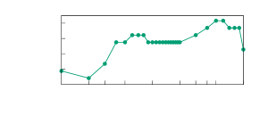
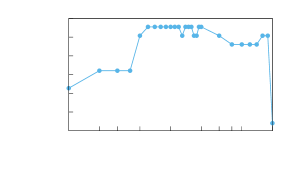
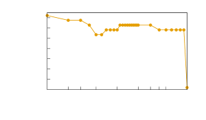
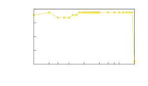
Figure 4, 5, 6, 7 and 8 present HR@1, HR@2, HR@3, HR@4 and HR@5 of - with over different values (Equation 2) when = 1 and = 1, respectively. As the weight increases from 0, that is, as the takes place in the term scoring (Equation 2), the performance of in terms of HR@1 and HR@2 generally increases. This demonstrates the effect from scoring component in . As further increases, the performance in general first gets better and then worse (except that the HR@1 performance reaches its best at =1). This indicates that the dynamic scoring component and scoring component in play complementary roles for recommending terms, and thus considering their combination enables better recommendation performance than each of the two methods alone.
Overall Performance on Other Cut-off Times
| statistics | INPC | ||||||||||||
|---|---|---|---|---|---|---|---|---|---|---|---|---|---|
| (06/26/2013) | (07/18/2013) | (08/15/2013) | (09/03/2013) | ||||||||||
| train | test | train | test | train | test | train | test | ||||||
| # | 13,819 | 6,669 | 587 | 8,471 | 624 | 10,852 | 472 | 12,014 | 372 | ||||
| # | 2,121 | 1,267 | 126 | 1,542 | 147 | 1,818 | 126 | 1,948 | 105 | ||||
| # | 9,781 | 5,334 | 665 | 6,550 | 654 | 7,952 | 532 | 8,657 | 461 | ||||
| # | 24,183 | 10,385 | 648 | 13,677 | 692 | 18,166 | 535 | 20,492 | 414 | ||||
| len() | 69,770 | 28,789 | 2,568 | 38,553 | 2,506 | 51,272 | 1,831 | 58,146 | 1,482 | ||||
| len()/# | 5.049 | 4.317 | 4.375 | 4.551 | 4.016 | 4.725 | 3.879 | 4.840 | 3.984 | ||||
| len()/# | 2.885 | 2.772 | 3.963 | 2.819 | 3.621 | 2.822 | 3.422 | 2.837 | 3.580 | ||||
-
•
In this table, # is the number of patients; # is the number of physicians; # is the number of terms; # is the number of sequences; len() is total length of sequences; len()/# is average length of sequences per patient and len()/# is average length of sequences.
Table 5 shows the dataset with different cut-off times 06/26/2013, 07/18/2013, 08/15/2013 and 09/03/2013. Table 6, Table 7 and Table 8 present the best performance of all the methods for cut-off time 06/26/2013, 07/18/2013 and 09/03/2013, respectively. Overall, - achieves the best performance over the other methods on the different cut-off times. The trends among different methods as identified from cut-off time 08/15/2013 remain very similar for the other cut-off times. Note that as using later cut-off times, training data become more as shown in Table 5, and the performance of each method over different cut-off times tends to become worse. For example, the performance of model decreases in general over different cut-off times. This may be due to the increasing heterogeneity among patients as more patients in the system.
| method | sim | HR@1 | HR@2 | HR@3 | HR@4 | HR@5 | |||||
| - | - | - | - | - | 0.205 | 0.313 | 0.341 | 0.369 | 0.381 | ||
| - | - | 0.261 | 0.366 | 0.380 | 0.383 | 0.383 | |||||
| - | - | 0.259 | 0.377 | 0.398 | 0.414 | 0.418 | |||||
| - | - | 0.250 | 0.373 | 0.403 | 0.418 | 0.431 | |||||
| - | - | 0.302 | 0.350 | 0.364 | 0.369 | 0.372 | |||||
| - | - | 0.287 | 0.370 | 0.397 | 0.414 | 0.421 | |||||
| - | - | 0.279 | 0.360 | 0.401 | 0.423 | 0.437 | |||||
| - | - | 0.262 | 0.349 | 0.397 | 0.421 | 0.444 | |||||
| - | - | - | 0.207 | 0.312 | 0.335 | 0.347 | 0.349 | ||||
| - | - | - | 0.204 | 0.313 | 0.343 | 0.350 | 0.353 | ||||
| - | - | - | 0.199 | 0.313 | 0.347 | 0.361 | 0.370 | ||||
| - | - | - | 0.194 | 0.312 | 0.346 | 0.356 | 0.372 | ||||
| - | - | 0.262 | 0.387 | 0.415 | 0.437 | 0.449 | |||||
| - | 0.253 | 0.377 | 0.420 | 0.449 | 0.458 | ||||||
| - | 0.258 | 0.381 | 0.420 | 0.449 | 0.460 | ||||||
| - | 0.262 | 0.370 | 0.407 | 0.438 | 0.455 | ||||||
| - | 0.219 | 0.380 | 0.409 | 0.440 | 0.469 | ||||||
| - | 0.227 | 0.375 | 0.417 | 0.441 | 0.463 | ||||||
| - | 0.216 | 0.363 | 0.412 | 0.451 | 0.463 | ||||||
| - | 0.228 | 0.373 | 0.417 | 0.443 | 0.475 | ||||||
| - | - | - | 0.215 | 0.310 | 0.352 | 0.381 | 0.392 | ||||
| - | - | 0.207 | 0.324 | 0.356 | 0.373 | 0.383 | |||||
| - | - | 0.208 | 0.312 | 0.360 | 0.384 | 0.394 | |||||
| - | - | 0.211 | 0.321 | 0.355 | 0.386 | 0.395 | |||||
| - | - | 0.208 | 0.318 | 0.353 | 0.381 | 0.397 |
-
•
In this table, the column “sim” corresponds to similarity identification methods; is the weight on CF component in ; is the number of similar patients; is the number of similar physicians; is the similarity threshold to identify similar terms. The best performance of each method under each metric is bold. The best overall performance of all methods under each metric is underlined.
| method | sim | HR@1 | HR@2 | HR@3 | HR@4 | HR@5 | |||||
| - | - | - | - | - | 0.210 | 0.292 | 0.325 | 0.341 | 0.348 | ||
| - | - | 0.267 | 0.347 | 0.358 | 0.364 | 0.366 | |||||
| - | - | 0.262 | 0.358 | 0.379 | 0.395 | 0.400 | |||||
| - | - | 0.257 | 0.358 | 0.384 | 0.402 | 0.412 | |||||
| - | - | 0.237 | 0.342 | 0.380 | 0.396 | 0.413 | |||||
| - | - | 0.289 | 0.337 | 0.353 | 0.357 | 0.358 | |||||
| - | - | 0.283 | 0.345 | 0.353 | 0.357 | 0.358 | |||||
| - | - | 0.240 | 0.325 | 0.379 | 0.410 | 0.426 | |||||
| - | - | - | 0.210 | 0.286 | 0.301 | 0.312 | 0.329 | ||||
| - | - | - | 0.207 | 0.289 | 0.305 | 0.318 | 0.329 | ||||
| - | - | - | 0.208 | 0.288 | 0.309 | 0.324 | 0.341 | ||||
| - | - | - | 0.208 | 0.288 | 0.308 | 0.325 | 0.340 | ||||
| - | - | 0.267 | 0.364 | 0.393 | 0.403 | 0.426 | |||||
| - | 0.256 | 0.355 | 0.396 | 0.415 | 0.428 | ||||||
| - | 0.253 | 0.360 | 0.396 | 0.413 | 0.431 | ||||||
| - | 0.251 | 0.347 | 0.387 | 0.408 | 0.426 | ||||||
| - | 0.250 | 0.351 | 0.392 | 0.413 | 0.431 | ||||||
| - | 0.228 | 0.341 | 0.397 | 0.419 | 0.441 | ||||||
| - | 0.228 | 0.335 | 0.389 | 0.423 | 0.436 | ||||||
| - | 0.212 | 0.315 | 0.384 | 0.412 | 0.447 | ||||||
| - | - | - | 0.218 | 0.292 | 0.332 | 0.351 | 0.367 | ||||
| - | - | 0.215 | 0.305 | 0.328 | 0.345 | 0.351 | |||||
| - | - | 0.217 | 0.302 | 0.340 | 0.355 | 0.364 | |||||
| - | - | 0.215 | 0.302 | 0.338 | 0.357 | 0.364 | |||||
| - | - | 0.208 | 0.292 | 0.331 | 0.354 | 0.367 |
-
•
In this table, the column “sim” corresponds to similarity identification methods; is the weight on CF component in ; is the number of similar patients; is the number of similar physicians; is the similarity threshold to identify similar terms. The best performance of each method under each metric is bold. The best overall performance of all methods under each metric is underlined.
| method | sim | HR@1 | HR@2 | HR@3 | HR@4 | HR@5 | |||||
| - | - | - | - | - | 0.193 | 0.271 | 0.304 | 0.331 | 0.365 | ||
| - | - | 0.261 | 0.326 | 0.345 | 0.355 | 0.355 | |||||
| - | - | 0.261 | 0.329 | 0.353 | 0.365 | 0.367 | |||||
| - | - | 0.246 | 0.324 | 0.374 | 0.399 | 0.406 | |||||
| - | - | 0.278 | 0.329 | 0.350 | 0.365 | 0.365 | |||||
| - | - | 0.271 | 0.336 | 0.360 | 0.379 | 0.384 | |||||
| - | - | 0.234 | 0.304 | 0.372 | 0.391 | 0.406 | |||||
| - | - | 0.242 | 0.331 | 0.362 | 0.396 | 0.408 | |||||
| - | - | 0.222 | 0.300 | 0.360 | 0.389 | 0.413 | |||||
| - | - | - | 0.184 | 0.246 | 0.271 | 0.290 | 0.304 | ||||
| - | - | - | 0.179 | 0.266 | 0.295 | 0.309 | 0.326 | ||||
| - | - | - | 0.174 | 0.261 | 0.312 | 0.338 | 0.353 | ||||
| - | - | 0.263 | 0.336 | 0.377 | 0.389 | 0.411 | |||||
| - | 0.261 | 0.338 | 0.377 | 0.389 | 0.411 | ||||||
| - | 0.234 | 0.331 | 0.382 | 0.411 | 0.425 | ||||||
| - | 0.246 | 0.331 | 0.382 | 0.408 | 0.428 | ||||||
| - | 0.242 | 0.319 | 0.355 | 0.386 | 0.423 | ||||||
| - | 0.234 | 0.343 | 0.384 | 0.391 | 0.418 | ||||||
| - | 0.234 | 0.336 | 0.389 | 0.396 | 0.423 | ||||||
| - | 0.220 | 0.333 | 0.374 | 0.403 | 0.425 | ||||||
| - | 0.208 | 0.312 | 0.362 | 0.391 | 0.435 | ||||||
| - | - | - | 0.208 | 0.292 | 0.326 | 0.348 | 0.374 | ||||
| - | - | 0.198 | 0.292 | 0.321 | 0.345 | 0.379 | |||||
| - | - | 0.181 | 0.271 | 0.338 | 0.365 | 0.382 | |||||
| - | - | 0.184 | 0.271 | 0.333 | 0.367 | 0.382 | |||||
| - | - | 0.198 | 0.278 | 0.319 | 0.350 | 0.389 |
-
•
In this table, the column “sim” corresponds to similarity identification methods; is the weight on CF component in ; is the number of similar patients; is the number of similar physicians; is the similarity threshold to identify similar terms. The best performance of each method under each metric is bold. The best overall performance of all methods under each metric is underlined.
Similarity Analysis
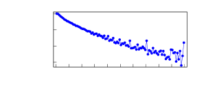
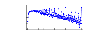
Figure 9 and 10 present the distribution of non-zero physician-physician similarities () and patient-patient similarities (), respectively. For , 5.65% of physician-physician similarities are non-zero, and 80.98% of the non-zero similarities are less than or equal to 0.2. For , 2.65% of the patient-patient similarities are non-zero, and 77.05% of the non-zero similarities are less than or equal to 0.5. Specially, there are some patients whose similarities with one another are relatively high (i.e., the peaks in Figure 10 on larger values). This also explains the advantages of over and their performance in Table 4, because more patients with higher to the target patient provide better opportunities for to identify relevant information from such similar patients.
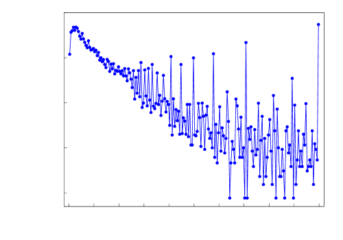
Figure 11 presents the distribution of non-zero term-term similarities (). For , only 0.28% of term-term similarities are non-zero, and 78.36% of the non-zero similarities are less than or equal to 0.3.
Conclusions
In this manuscript, we presented our new dynamic and multi-collaborative filtering method to recommend search terms relevant to patients for physicians. combines a dynamic first-order Markov chain model and a multi-collaborative filtering model in order to score and prioritize search terms. The collaborative filtering model leverages the key idea originating from Recommender Systems research, and uses patient similarities, physician similarities and term similarities to score potential search terms. The linear combination of the dynamic-based scoring and the multi-collaborative filtering-based scoring is able to produce high quality recommendations that are most relevant to the patients and that are most interested to physicians.
Acknowledgment
This project was made possible, in part, by support from the National Science Foundation under Grant Number IIS- 1855501 and IIS-1827472, and from National Library of Medicine under Grant Number 1R01LM012605-01A1. Any opinions, findings, and conclusions or recommendations expressed in this material are those of the authors and do not necessarily reflect the views of the funding agencies.
References
- 1. Ricci F, Rokach L, Shapira B. Recommender systems handbook. 2nd ed. Springer Publishing Company, Incorporated; 2015.
- 2. Ning X, Desrosiers C, Karypis G. A comprehensive survey of neighborhood-based recommendation methods. In: Ricci F, Rokach L, Shapira B, editors. Recommender Systems Handbook. Boston, MA: Springer US; 2015. p. 37–76.
- 3. Zhang S, Yao L, Sun A. Deep learning based recommender system: a survey and new perspectives; 2017.
- 4. Zhang C, Wang K, Yu H, Sun J, Lim EP. Latent factor transition for dynamic collaborative filtering. In: Proceedings of the 2014 SIAM International Conference on Data Mining. SIAM; 2014. p. 452–460.
- 5. Sahoo N, Singh PV, Mukhopadhyay T. A hidden markov model for collaborative filtering. Mis Quarterly. 2012; p. 1329–1356.
- 6. Sun JZ, Varshney KR, Subbian K. Dynamic matrix factorization: a state space approach. In: Acoustics, Speech and Signal Processing (ICASSP), 2012 IEEE International Conference on. IEEE; 2012. p. 1897–1900.
- 7. Sun JZ, Parthasarathy D, Varshney KR. Collaborative kalman filtering for dynamic matrix factorization. IEEE Trans Signal Processing. 2014;62(14):3499–3509.
- 8. Luo D, Xu H, Zhen Y, Ning X, Zha H, Yang X, et al. Multi-task multi-dimensional Hawkes processes for modeling event sequences. In: Proceedings of the 24th International Joint Conference on Artificial Intelligence. IJCAI’15; 2015. p. 3685–3691.
- 9. Xiong L, Chen X, Huang TK, Schneider J, Carbonell JG. Temporal collaborative filtering with bayesian probabilistic tensor factorization. In: Proceedings of the 2010 SIAM International Conference on Data Mining. SIAM; 2010. p. 211–222.
- 10. Wiesner M, Pfeifer D. Health recommender systems: concepts, requirements, technical basics and challenges. International Journal of Environmental Research and Public Health. 2014;11(3):2580–2607. doi:10.3390/ijerph110302580.
- 11. Guo L, Jin B, Yao C, Yang H, Huang D, Wang F. Which doctor to trust: a recommender system for identifying the right doctors. Journal of medical Internet research. 2016;18(7).
- 12. Jiang H, Xu W. How to find your appropriate doctor: an integrated recommendation framework in big data context. In: Computational Intelligence in Healthcare and e-health (CICARE), 2014 IEEE Symposium on. IEEE; 2014. p. 154–158.
- 13. Zhang Q, Zhang G, Lu J, Wu D. A framework of hybrid recommender system for personalized clinical prescription. In: 2015 10th International Conference on Intelligent Systems and Knowledge Engineering (ISKE); 2015. p. 189 – 195.
- 14. Bao Y, Jiang X. An intelligent medicine recommender system framework. In: Industrial Electronics and Applications (ICIEA), 2016 IEEE 11th Conference on. IEEE; 2016. p. 1383–1388.
- 15. Gräßer F, Malberg H, Zaunseder S, Beckert S, Küster D, Schmitt J, et al. Application of recommender system methods for therapy decision support. In: 2016 IEEE 18th International Conference on e-Health Networking, Applications and Services (Healthcom); 2016. p. 1–6.
- 16. Duan L, Street WN, Xu E. Healthcare information systems: data mining methods in the creation of a clinical recommender system. Enterprise Information Systems. 2011;5(2):169–181.
- 17. Moffett P, Moore G. The standard of care: legal history and definitions: the bad and good news. Western Journal of Emergency Medicine. 2011;12(1):109.
- 18. Lewis MH, Gohagan JK, Merenstein DJ. The locality rule and the physician’s dilemma: local medical practices vs the national standard of care. JAMA. 2007;297(23):2633–2637.
- 19. Norris JR. Markov chains. 2. Cambridge university press; 1998.
- 20. Aggarwal CC, Zhai C. Mining text data. Springer Science & Business Media; 2012.