Full Reference Screen Content Image Quality Assessment by Fusing Multi-level Structure Similarity

Abstract.

The screen content images (SCIs) usually comprise various content types with sharp edges, in which the artifacts or distortions can be well sensed by the vanilla structure similarity measurement in a full reference manner. Nonetheless, almost all of the current SOTA structure similarity metrics are “locally” formulated in a single-level manner, while the true human visual system (HVS) follows the multi-level manner, and such mismatch could eventually prevent these metrics from achieving trustworthy quality assessment. To ameliorate, this paper advocates a novel solution to measure structure similarity “globally” from the perspective of sparse representation. To perform multi-level quality assessment in accordance with the real HVS, the above-mentioned global metric will be integrated with the conventional local ones by resorting to the newly devised selective deep fusion network. To validate its efficacy and effectiveness, we have compared our method with 12 SOTA methods over two widely-used large-scale public SCI datasets, and the quantitative results indicate that our method yields significantly higher consistency with subjective quality score than the currently leading works. Both the source code and data are also publicly available to gain widespread acceptance and facilitate new advancement and its validation.

1. Introduction and Motivation

As one of the most informative representation venues, the screen content images (SCIs) are ubiquitous in various multimedia devices, such as mobile phone, laptop, tablet, and so on (Chen et al., 2018a; Fang et al., 2018; Miao et al., 2016; Chen et al., 2016b, 2015a; Hu et al., 2014). From the perspective of the multi-client communication systems, the SCIs received by multimedia may usually get distorted during acquisition, storage, transmission, and coding (Ma et al., 2014; Zhu et al., 2015; Chang et al., 2014) Thus, it is of very importance to design an effective quality assessment method for SCIs.

In fact, the image quality assessment (IQA) problem has been paid intensive research attention during the past several years. According to the availability of the reference image, the state-of-the-art (SOTA) IQA methods (Gu et al., 2017b; Zhou et al., 2018) can be roughly grouped into three categories: the full reference, the reduced reference, and the no reference methods (Qian et al., 2017; Min et al., 2017; Freitas et al., 2018), where the first two of these three would need to know the full or partial undistorted image respectively, while the last one would not. In order to pay attention to this paper’s main foci, we only shed light on the topic of full reference with brief justification and discussion.

In essence, most of the existing full reference IQA methods are designed for the natural scene images (NSIs). Nonetheless, different from the NSIs which usually comprise image content with gradual variations, the SCIs are frequently synthesized and rendered, exhibiting image content with sharp edges (Wang et al., 2016, 2015). Furthermore, the image content type of SCIs is also different from NSIs, i.e., the NSIs mainly relate to pictures, while the SCIs contain both pictures and textures. Thus, the NSIs based methods are not feasible for the SCIs (Ni et al., 2016a).

As for the current main stream full reference methods for SCIs, the structure similarity (Wang et al., 2004) has been widely adopted to sense artifacts in distorted images, and a strong similarity between the reference SCI and its distorted version usually indicates a high quality score, and vice versa. Although much more progresses have been made, almost all the structure similarity measurement based variants are locally formulated (Gu et al., 2016; Ni et al., 2017), which could easily produce untrustworthy quality assessment due to its limited sensing scope (e.g., conducing IQA via patch-wise or regional-wise manner, please refer to Fig. 1-A). Moreover, most of the current SOTA works shall be classified into the single-level category, in which these works solely use either local or global measurement each time. However, such “single-level” manner principally contradicts to the “multi-level” real human visual system (HVS) which shifts intermittently between the entire image sweeping and the tiny artifact zooming, preventing the SOTA methods from performing trustworthy quality assessment. Additionally, the image content type is another vital factor to affect the overall performance (Zhang et al., 2018), which should be considered when pursuing a trustworthy quality assessment.

Hence, all the above-mentioned arguments motivate us to investigate a multi-level manner for the SCI quality assessment, which mainly includes the following three aspects: low-level structure-aware metrics, mid-level image content, and high-level selective fusion. Meanwhile, since the SCIs can be attributed to a mixture of textures and pictures, the HVS frequently pays more attention to the irregular patterns (e.g., miss-aligned textures), thus the tiny structure distortions may easily be observed by the HVS (Chen et al., 2016a; Ma et al., 2019; Chen et al., 2019, 2020). Therefore, it is intuitive to choose the structure similarity as the “low-level” metric to detect distortion induced artifacts. To compute the structure similarity globally, we utilize the sparse representation (Aharon et al., 2006) to sequentially formulate the structure consistency of the reference SCI as the global structure dictionary. By using this dictionary to respectively reconstruct the reference SCI and its distorted version, we can use the variation degree toward dictionary usage to represent the global structure similarity (please refer to Fig. 1-B). Meanwhile, we integrate the off-the-shelf local structure similarity into our newly devised global one by using our newly designed “high-level” fusion network. To realize the “mid-level” content-aware attribute, we divide the target SCI into partially overlapped texture/picture patches with the fixed patch size, and then these patches will be individually feeded into the subsequent fusion network, avoiding the resizing operation induced distortions. In summary, we list the salient contributions as follows:

$\bullet$ We propose to conduct full reference quality assessment for SCIs in a multi-level manner, which is perceptually consistent with the real multi-level HSV;

$\bullet$ We propose a novel sparse representation based metric to measure structure similarity globally, which can effectively complement to the conventional local measurement for a trustworthy quality assessment;

$\bullet$ We design a novel selective deep fusion network to integrate the local and global structure similarity towards a high-level processing and understanding, giving rise to much better accuracy than the conventional hand-crafted solutions;

$\bullet$ We newly devise a novel content-aware decomposition scheme to further improve the robustness of our SCI quality assessment;

$\bullet$ The source code and results are publicly available at https://github.com/HongmengZhao/SR-CNN.

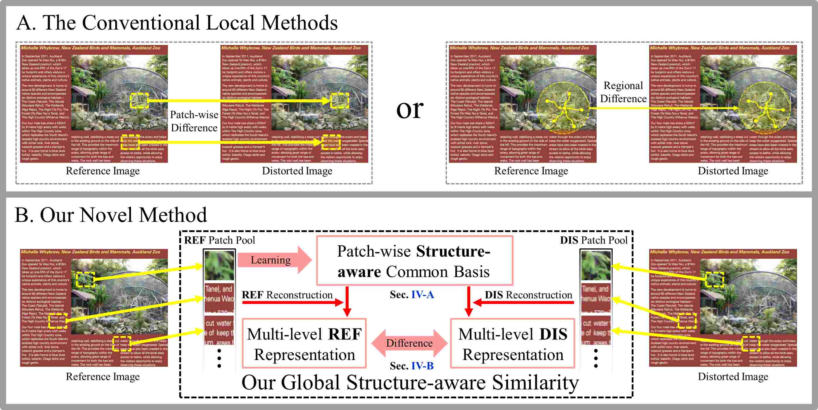
Figure 1. The conventional methods frequently resort the single-level fashion for IQA, e.g., solely using patch-wise or regional-wise manner to sense distortion induced artifacts, which contradicts to the multi-level real HVS. In sharp contrast, this paper proposes to conduct measure the structure-aware similarity globally, which particulary suits the quality assessment for SCIs (Wang et al., 2004; Gu et al., 2015). The abbreviation “REF” and “DIS” respectively denote the reference image and the distorted image.

2. related work

Most of the existing FR (Full Reference) IQA methods are designed for natural scene images (NSIs), which frequently utilize pixel-wise measurements to evaluate the differences between the reference image and its distorted version. Thus, the sensed differences, which is positively related to the distortion level, can be used to predict the overall quality score.

2.1. Structure Similarity Metrics

As a milestone FR metric for NSIs, Zhou et al. (Wang et al., 2004) conducts IQA mainly from the structural similarity (SSIM) perspective, which is inspired from the phenomenon that the HVS is highly sensitive to structural information, and multiple improved subsequent works are proposed latter (Wang and Li, 2011; Zhang et al., 2013; Xue et al., 2014). Different from the quality assessment of NSIs, the existence of various image content types in SCIs (e.g. computer generated textures and graphics) makes the quality assessment more challenging. To appropriately reveal the correlation between the SSIM captured artifacts and the overall quality scores, Gu et al. (Gu et al., 2015) proposes to re-weight the classic SSIM (Wang et al., 2004) with structural degradation measurement computed using SSIM on the original SCI and its distorted version via a low-pass filter. Moreover, since the HVS may pay more attention to salient object (Chen et al., 2015b, 2017, 2018b; Li et al., 2019), Gu et al. (Gu et al., 2016) further integrates the structural degradation measurement with structure variation based saliency clue to improve the overall quality score. To better perceive structural degradation, Ni et al. (Ni et al., 2016a) proposes to utilize both gradient direction and gradient magnitude to yield the overall quality assessment by employing a deviation-based pooling strategy, which is further improved by adopting the weighted pooling scheme to fuse the edge contrast degree with edge width variation (Ni et al., 2016b). Meanwhile, the above-mentioned edge information can also be expanded to simultaneously consider edge contrast, edge width and edge direction (Ni et al., 2017). Since the Gabor filters are highly consistent with the response of the HVS, Ni et al. (Ni et al., 2018) resorted the Gabor filter to measure the global similarity between the reference image and its distorted version, achieving much improved quality assessment performance.

2.2. Content-aware Fusion

Despite the above-mentioned efforts to investigate low-level venues in accordance to the real HVS, these approaches may not be able to perform well occasionally due to its less consideration of the content types of the given SCIs. Thus, Yang et al. (Yang et al., 2015) proposes to separately measure sharpness similarity for image regions with different content types, i.e., texture regions and picture regions. Similarly, Wang et al. (Wang et al., 2016) proposed to incorporate both visual field adaptation and information content weighting into structural similarity based local quality assessment by adopting the information content model (Wang and Shang, 2006). Since the distortion metrics are computed individually on different content types, Fang et al. (Fang et al., 2017) proposes to use the uncertainty weighting scheme to fuse the visual quality of textual and pictorial regions effectively, achieving remarkable performance improvement. Although the above mentioned works have improved the quality assessment performance significantly, its hand-crafted nature has a tendency to reach performance bottle neck.

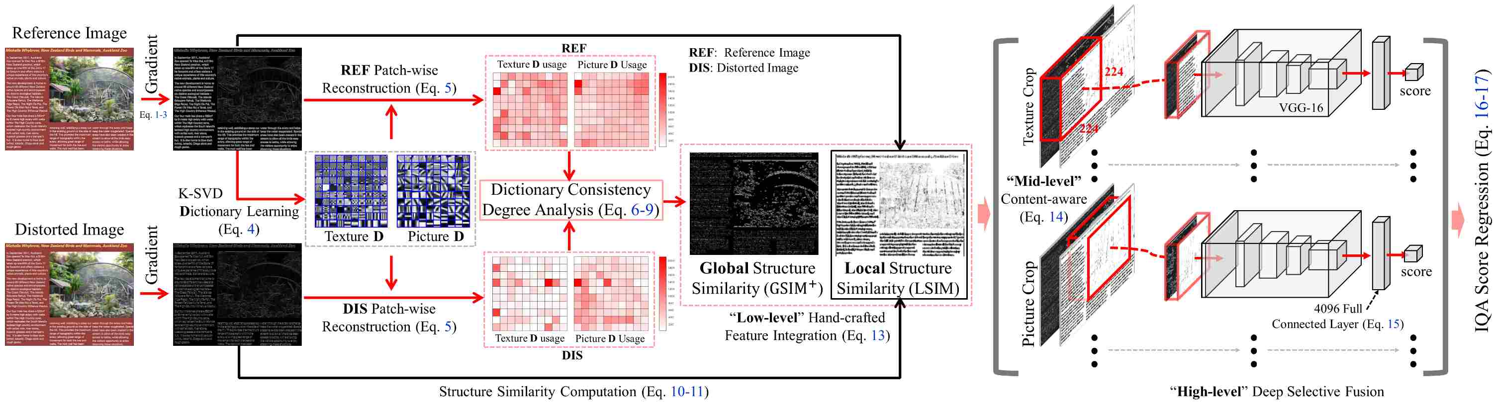
Figure 2. The overall pipeline of our proposed multi-level SR-CNN method. The left part shows the “low-level” local/global structure-aware similarity measurement (Sec. 4), and the right part demonstrates the “mid-level” content-aware patch selection and the “high-level” selective deep fusion toward the optimal quality score regression (Sec. 5).

2.3. Deep Learning based Methods

After entering the deep learning era, multiple convolutional neural networks (CNNs) based methods have been developed to solve the IQA problem for SCIs. For instance, Zuo et al. (Zuo et al., 2016) proposes to directly input the sequentially cropped patches into CNNs to automatically reveal deep features for its subsequent quality score regression. To shrink the regression problem domain, Cheng et al. (Cheng et al., 2018) adopts a predefined saliency threshold to assign lower weight to the relatively less salient patches. Different form pervious works which solely divide SCIs into texture and picture regions, Zhang et al. (Zhang et al., 2018) proposes to employ CNNs-based content classifier to assign image regions into a novel SCI content, i.e., computer-graphics/cartoons. Although this newly introduced content type is actually in line with the real HVS, it still follows the conventional hand-crafted manner to conduct its subsequent quality assessment with limited accuracy. Also, the NSIs based deep models can be adapted for SCIs by using the off-the-shelf naturalization deep network, inducing significant performance improvement (Jiang et al., 2019b), in which Chen et al. (Chen et al., 2018c) uses the naturalization module to transform IQA of SCIs into IQA of NSIs. Most recently, Jiang et al. (Jiang et al., 2019b) proposes a quadratic optimized model to select representative image patches from the pre-trained deep model, and thus the quality assessment results predicted by this method are relatively more close to the DMOS (Differential Mean Opinion Score).

In summary, compared to the hand-crafted methods, the above mentioned deep learning based works have achieved significant performance improvements, however, almost all these methods still follow the single-level or bi-level fashions, contradicting to the real HVS using multi-level clues in practice. Thus, all the mentioned above motivates us to use deep learning framework to selectively integrate multi-level metrics for a high performance SCI quality assessment.

3. Method Overview

As shown in Fig. 2, our method mainly consists of two stages: 1) Structure-aware global feature computation; 2) Global and local deep selective fusion. Given a reference SCI (screen content image), we propose to conduct patch-wise dictionary learning to obtain multiple “structure-aware” non-local basis. To achieve it, we conduct the accelerated K-SVD (Aharon et al., 2006) algorithm over the reference gradient image to formulate a 100-codeword dictionary respectively for texture (see Texture D in Fig. 2) and picture regions (see Picture D in Fig. 2). Since the learned dictionaries can globally represent the consistent non-local structures of the reference image, we propose to globally predict the distortion degree of the given input image by measuring the differences between its codeword usage and the codeword usage in its reference image. Meanwhile, we also adopt the local structure similarity measurement to complement the above-mentioned global one. In particular, we adopt the newly designed selective deep fusion network for an optimal fusion state between these two measurements, achieving accurate IQA predictions eventually.

4. Structure-aware Similarity Features Computation

Given a reference image (REF) and its distorted version (DIS), we first formulate its non-local basis (codewords) by conducting the K-SVD learning procedure. Next, from the codeword usage perspective, we measure the differences between REF and DIS to represent our structure-aware global similarity.

4.1. Preliminaries

In general, for any screen content image (I), its structural information can be represented by using its two directional gradient maps ($G(\textbf{I})$), which can be formulated as Eq. 1.

(1) $$G(\textbf{I})=\sqrt{(h_{x}*\textbf{I})^{2}+(h_{y}*\textbf{I})^{2}},$$

where $h_{x}=[-\frac{1}{2}\ 0\ \frac{1}{2}]$ and $h_{y}=[-\frac{1}{2}\ 0\ \frac{1}{2}]^{\rm T}$ denote the vertical kernel and horizonal kernel respectively, and the operator $*$ denotes the convolution operation. So, given a pair of reference image ($\textbf{I}_{r}$) and its distorted version ($\textbf{I}_{d}$), we can represent their gradient maps respectively as $G(\textbf{I}_{r})$ and $G(\textbf{I}_{d})$.

To obtain the global structure-aware dictionary of the reference image, we first adopt the patch-wise decomposition (patch size: $8\times 8$, overlapping rate: 50%) over $\textbf{I}_{r}$ and then learn the common structure basis from these segmented image patches. To balance the trade-off between computational cost and performance, we randomly select maximum 20,000 texture patches and maximum 20,000 picture patches to respectively formulate the texture dictionary (with 100 codewords) and picture dictionary (with 100 codewords), in which we adopt the off-the-shelf method (Jaderberg et al., 2014) to separate texture patches from picture patches.

Here we represent the selected patch-wise texture/picture data respectively as Eq. 2/Eq. 3.

(2) $$\textbf{Y}_{rt}=\{\textbf{t}_{1},\textbf{t}_{2},...,\textbf{t}_{TN}\}\in\mathbb{R}^{64\times TN},$$

(3) $$\textbf{Y}_{rp}=\{\textbf{p}_{1},\textbf{p}_{2},...,\textbf{p}_{PN}\}\in\mathbb{R}^{64\times PN},$$

where $t$ and $p$ respectively denote the columnized texture patches and the columnized picture patches, $TN\leq 20,000$ and $PN\leq 20,000$ respectively denote the total number of the selected texture/picture patch numbers in practice. Thus, the dictionaries learning procedure can be formulated as Eq. 4.

(4) $$\min\limits_{\textbf{D}_{t/p},\textbf{X}_{t/p}}\parallel\textbf{Y}_{t/p}-\textbf{D}_{t/p}\cdot\textbf{X}_{t/p}\parallel_{F}^{2},\ \ \ s.t.\ \ \forall i,\parallel\textbf{x}_{i}\parallel_{0}\leq\rm T_{0},$$

where $\textbf{D}_{t}$ and $\textbf{D}_{p}$ respectively denote the texture dictionary and the picture dictionary with total 100 dictionary atoms ($\textbf{D}_{t/p}\in\mathbb{R}^{64\times 100}$), $\textbf{X}=\{\textbf{x}_{1},\textbf{x}_{2},...,\textbf{x}_{TNorPN}\}\in\mathbb{R}^{100\times(TN\ or\ PN)}$ is a sparse matrix representing the dictionary usage toward the input Y.

Actually, Eq. 4 is a common thread of the sparse representation problem (Peng et al., 2019, 2020), where the left Frobenius norm ensures a minimization of the reconstructed mean standard error while the right part constraint maintain a sparse state toward the dictionary atom usage. Thus, Eq. 4 can be alternative solved, i.e., we utilize SVD decomposition to iteratively estimate D, and then the code matrix X can be obtained by using the orthogonal matching pursuit (OMP (Pati et al., 1993)) over the current generated dictionary D. In this way, we can easily obtain a complete high-quality dictionary and its corresponding sparse coding. Also, we demonstrate the difference between the learned texture dictionary ($\textbf{D}_{t}$) and picture dictionary ($\textbf{D}_{p}$) in Fig. 3.

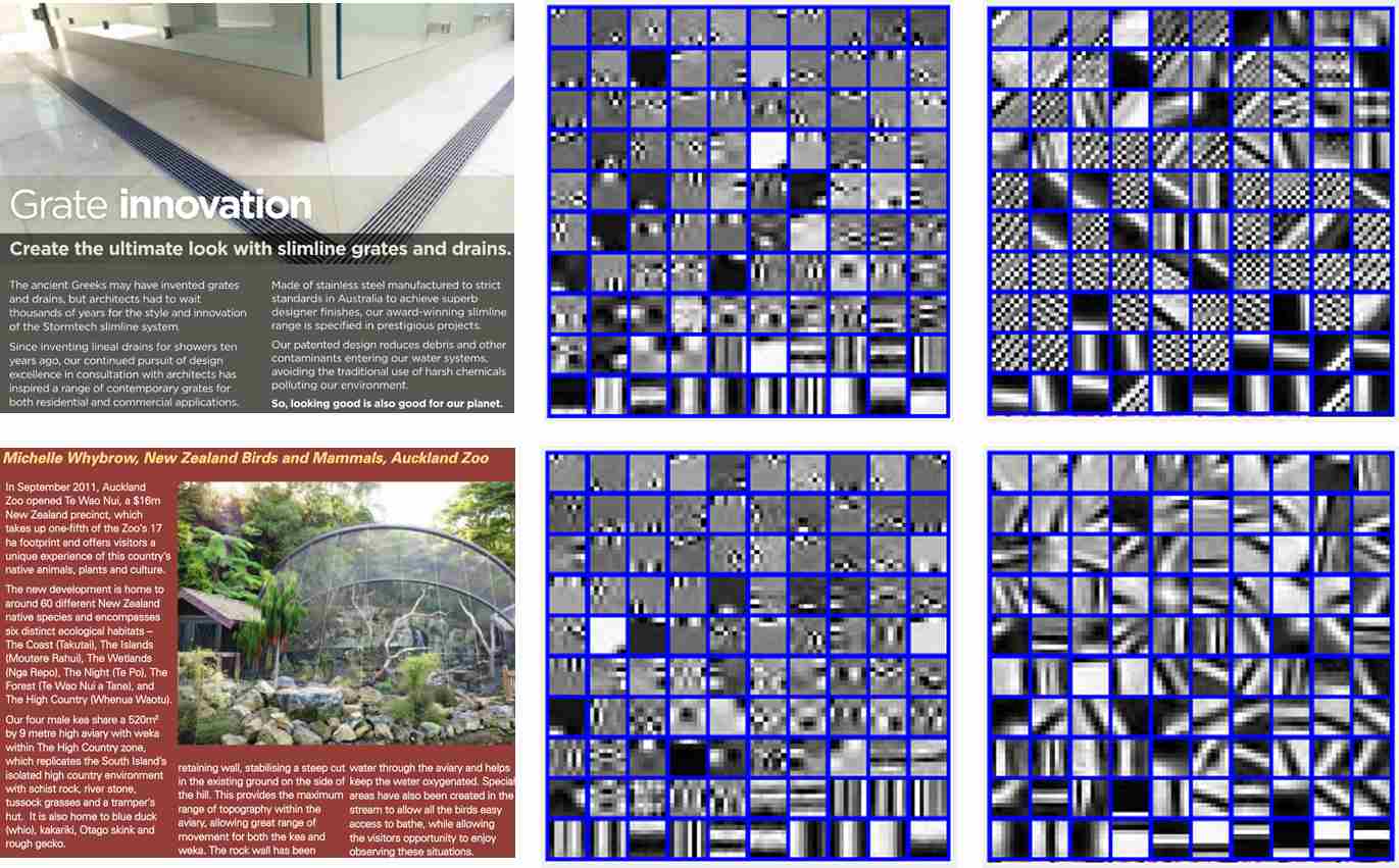
Figure 3. An illustration of the revealed textual/picture dictionaries. [Column 1]: reference SCIs. [Column 2]: the corresponding texture dictionaries. [Column 3]: the corresponding picture dictionaries.

4.2. Multi-level Structure-aware Similarity

Since the SCIs (screen content images) frequently exhibit sharp boundaries, the conventional “local” structure similarity has been widely adopted to measure the distortion degree of the input image. However, such “local” protocol may contradict with the real HVS (human visual system) in the following two aspects:
1) The HVS may easily overlook the structure related tiny distortions in cluttered backgrounds;
2) Moreover, our HVS tends to sweep though the entire screen while assigning an objective SCI score.

To satisfy the former attribute 1), we propose to limit the structure similarity measurement scope within the common basis $\textbf{D}_{t/p}$ which are previously obtained from the reference SCI via Eq. 4. Thus, the tiny structure distortions can be automatically filtered during the IQA process. Meanwhile, as for the attribute 2), we propose to conduct IQA by measuring the structure similarity from the “global” perspective, in which we reconstruct the distorted image over $\textbf{D}_{t/p}$, and then measure the dictionary usage consistency degree between REF (reference image) and DIS (distorted image) as the predicted image quality degree.

Suppose we have already obtained the reference texture dictionary ($\textbf{D}_{t}^{r}$) and the reference picture dictionary ($\textbf{D}_{p}^{r}$), the reconstruction procedure toward the distorted image can be formulated as Eq. 5.

(5) $$\min\limits_{\textbf{X}_{t/p}^{d}}\parallel\textbf{Y}_{t/p}^{d}-\textbf{D}_{t/p}^{r}\cdot\textbf{X}_{t/p}^{d}\parallel_{F}^{2},\ \ \ s.t.\ \ \forall i,\parallel\textbf{x}_{i}\parallel_{0}\leq\rm T_{0},$$

where the superscript $r$ and $d$ denote the reference image and the distorted image, respectively. We also have adopted the (Zhou et al., 2018) proposed $k$ nearest clustering strategy to accelerate the reconstruction procedure. By reconstructing the distorted image over the structure dictionary provided by reference (Eq. 4), we can obtain the sparse coding of the distorted image, i.e., the distorted texture coding ($\textbf{X}_{t}^{d}$) and the distorted picture coding ($\textbf{X}_{p}^{d}$). Actually, the sparse coding of the distorted image is partially different to the sparse coding of the reference image, which can well perceive the distinction between reference and distorted SCIs. Thus, we utilize the dictionary atom usage overlapping rate to measure the distortion degree, in which both the $\textbf{X}_{t/p}^{d}$ and the $\textbf{X}_{t/p}^{r}$ are negatively related to the distortion degree. Here we formulate such computation process as Eq. 6.

(6) $$\rm{GSIM}_{\emph{t/p}}(\emph{i}) =\frac{\parallel\emph{col}(\textbf{X}_{\emph{t/p}}^{\emph{d}}\cdot\textbf{X}_{\emph{t/p}}^{\emph{r}},\emph{i})\parallel_{0}}{\parallel\emph{col}(\textbf{X}_{\emph{t/p}}^{\emph{d}},\emph{i})\parallel_{0}+\parallel\emph{col}(\textbf{X}_{\emph{t/p}}^{\emph{r}},\emph{i})\parallel_{0}}$$

$$=\frac{\parallel\emph{col}({\left[\begin{smallmatrix}\textbf{x}_{\emph{1,1}}^{\emph{d}}&\cdots&\textbf{x}_{\emph{1,TN/PN}}^{\emph{d}}\\ \vdots&\vdots&\vdots\\ \textbf{x}_{\emph{100,1}}^{\emph{d}}&\cdots&\textbf{x}_{\emph{100,TN/PN}}^{\emph{d}}\\ \end{smallmatrix}\right]}\cdot{\left[\begin{smallmatrix}\textbf{x}_{\emph{1,1}}^{\emph{r}}&\cdots&\textbf{x}_{\emph{1,TN/PN}}^{\emph{r}}\\ \vdots&\vdots&\vdots\\ \textbf{x}_{\emph{100,1}}^{\emph{r}}&\cdots&\textbf{x}_{\emph{100,TN/PN}}^{\emph{r}}\\ \end{smallmatrix}\right]},\emph{i})\parallel_{0}}{\parallel\emph{col}({\left[\begin{smallmatrix}\textbf{x}_{\emph{1,1}}^{\emph{d}}&\cdots&\textbf{x}_{\emph{1,TN/PN}}^{\emph{d}}\\ \vdots&\vdots&\vdots\\ \textbf{x}_{\emph{100,1}}^{\emph{d}}&\cdots&\textbf{x}_{\emph{100,TN/PN}}^{\emph{d}}\\ \end{smallmatrix}\right]},\emph{i})\parallel_{0}+\parallel\emph{col}({\left[\begin{smallmatrix}\textbf{x}_{\emph{1,1}}^{\emph{r}}&\cdots&\textbf{x}_{\emph{1,TN/PN}}^{\emph{r}}\\ \vdots&\vdots&\vdots\\ \textbf{x}_{\emph{100,1}}^{\emph{r}}&\cdots&\textbf{x}_{\emph{100,TN/PN}}^{\emph{r}}\\ \end{smallmatrix}\right]},\emph{i})\parallel_{0}}$$

where the global texture structure similarity $\rm{GSIM}_{\emph{t}}\in\mathbb{R}^{1\times\emph{TN}}$, and the picture structure similarity $\rm{GSIM}_{\emph{p}}\in\mathbb{R}^{1\times\emph{PN}}$, $TN$ and $PN$ respectively denote the number of selected texture and picture patches, function $col(\textbf{X},i)$ returns the $i$-th column of its input matrix X, $\parallel\cdot\parallel_{0}$ denotes the $l_{0}$-norm.

So far, the computed GSIM (Eq. 6) can well measure the global structure similarity from the perspective of sparse reconstruction. Meanwhile, to further measure the structure similarity from the dictionary perspective (further strengthen the global attribute), we propose to introduce the dictionary atom usage coefficients into Eq. 6 as its patch-wise weights, because the dictionary atoms with large coefficient variations should be considered more during the above-mentioned measurement, and vice versa. Here we formulate the patch-wise dictionary atom weight as Eq. 7.

(7) $$\begin{split}\rm{CW}_{\emph{t/p}}(\emph{i})=\underset{overlapped\ atom\ mask}{\underbrace{\lceil\frac{\emph{col}(\textbf{X}_{\emph{t/p}}^{\emph{d}}\cdot\textbf{X}_{\emph{t/p}}^{\emph{r}},\emph{i})}{\max\{\emph{col}(\textbf{X}_{\emph{t/p}}^{\emph{d}}\cdot\textbf{X}_{\emph{t/p}}^{\emph{r}},\emph{i})\}}\rceil}}\cdot\underset{coefficient\ change}{\underbrace{\frac{|\textbf{C}_{\emph{t/p}}^{\emph{d}}-\textbf{C}_{\emph{t/p}}^{\emph{r}}|}{|\textbf{C}_{\emph{t/p}}^{\emph{d}}|+|\textbf{C}_{\emph{t/p}}^{\emph{r}}|}}},\end{split}$$

In Eq. 7, $\lceil\cdot\rceil$ denotes the ceiling operation; The left part $\in\{0,1\}$ indicates the overlapped dictionary atom usage toward the $i$-th image patch, while the right part measures the difference of the dictionary usage coefficient (C), which can be formulated by Eq. 8.

(8) $$\textbf{C}_{\emph{t}}^{\emph{d/r}}=\rm\frac{\sum(\textbf{X}_{\emph{t}}^{\emph{d/r}})}{\emph{TN}},\ \ \ \ \textbf{C}_{\emph{p}}^{\emph{d/r}}=\rm\frac{\sum(\textbf{X}_{\emph{p}}^{\emph{d/r}})}{\emph{PN}},$$

where the superscript $d/r$ denotes the reference image or the distorted image, $\textbf{C}\in\mathbb{R}^{1\times{TN\ or\ PN}}$ denotes the dictionary atom usage variation, and function $\sum$ represents the column-wise summation.

At this point, we can re-formulate Eq. 6 into the following Eq. 9.

(9) $$\rm{GSIM}^{+}_{t/p}(i)=\{CW_{\emph{t/p}}(i)\}^{\alpha_{1}}\cdot\{\rm{GSIM}_{\emph{t/p}}(i)\}^{\beta_{1}},$$

where $\alpha_{1}$ and $\beta_{1}$ are two predefined parameters to control the balance between the dictionary coefficient component and the dictionary overlapping component. In this paper, these two parameter values are empirically assigned to $\alpha_{1}=0.2$ and $\beta_{1}=1$.

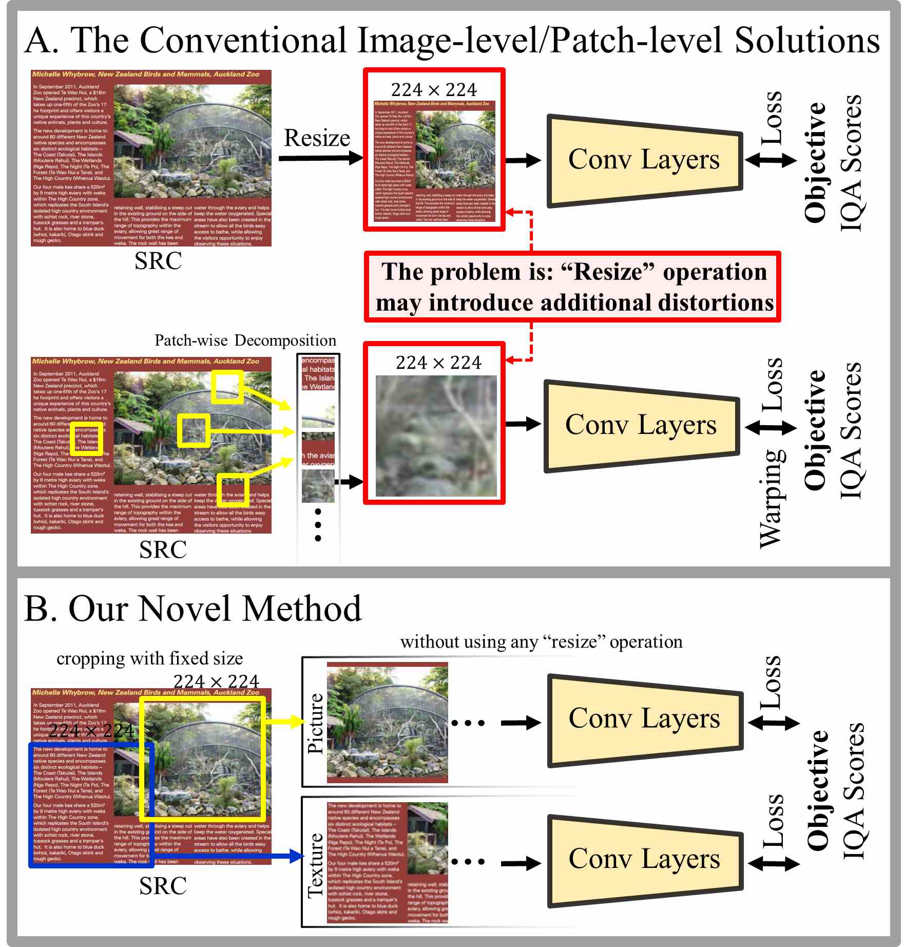
Figure 4. The current main stream deep learning based methods (Jiang et al., 2019b; Chen et al., 2018c) frequently resort the “resize” operation to adapt patch-wise input data for their pre-trained feature backbones, which is inevitable to bring additional distortions, making the quality score regression difficult. So, we adopt the content-aware patch selection (Sec. 5.1) to solve this problem.

Meanwhile, though the $\rm{GSIM}^{+}_{t/p}$ can well represent the global structure similarity already, yet the local structure similarity should also be considered, because the HVS may also be easily attracted to the conspicuous tiny local structure artifacts in plain texture regions. Therefore, inspired by the conventional structure similarity computations (Liu et al., 2012; Zhang et al., 2014; Xing et al., 2017), we propose to formulate our local structure similarity computation between the reference gradient map ($G(\textbf{I}^{r})$, Eq. 1) and the distorted gradient map ($G(\textbf{I}^{d})$, Eq. 1) within a patch-wise manner as Eq. 10.

(10) $$\begin{split}\rm{LSIM}&(i)=\\ &\frac{\mu^{r}_{i}\cdot\mu^{d}_{i}+\rm{C}_{1}}{\{\mu^{r}_{i}\}^{2}+\{\mu^{d}_{i}\}^{2}+\rm{C}_{1}}\cdot\frac{\sigma^{r}_{i}\cdot\sigma^{d}_{i}+\rm{C}_{2}}{\{\sigma^{r}_{i}\}^{2}+\{\sigma^{d}_{i}\}^{2}+\rm{C}_{2}},\end{split}$$

where $\mu_{i}$ and $\sigma_{i}$ respectively denote the mean value and the standard value of the $i$-th gradient patch, which can be formulated by Eq. 11, $\rm C_{1}$ and $\rm C_{2}$ are two constant values to avoid the instability in the case that the denominator is close to zero, i.e., $\rm C1=(0.01*255)^{2}$ and $\rm C2=(0.03*255)^{2}$.

(11) $$\mu^{r/d}_{i}=mean\{\emph{col}(\textbf{Y}^{r/d},i)\},\ \sigma^{r/d}_{i}=std\{\emph{col}(\textbf{Y}^{r/d},i)\}.$$

The patch-wise quality assessment score (PS) can be computed by using multiplicative based fusion toward $\rm GSIM^{+}$ (Eq. 9) and $\rm LSIM$ (Eq. 10) as the following:

(12) $$\rm{PS}(\emph{i})=\left\{\begin{array}[]{ll}\{\rm{LSIM}(\emph{i})\}^{\alpha_{2}}\cdot\{\rm{GSIM}^{+}_{\emph{t}}(\emph{i})\}^{\beta_{2}}\ \ \ \emph{if}\ \emph{i}\in\textbf{Y}_{\emph{t}}\\ \{\rm{LSIM}(\emph{i})\}^{\alpha_{2}}\cdot\{\rm{GSIM}^{+}_{\emph{p}}(\emph{i})\}^{\beta_{2}}\ \ \ \emph{if}\ \emph{i}\in\textbf{Y}_{\emph{p}}\\ \end{array}\right.,$$

where $\alpha_{2}=0.6$ and $\beta_{2}=1$ are another two pre-defined weighting parameters to control the balance between the LSIM and $\rm GSIM^{+}$. Then, the image level quality assessment score (FSIM) can be obtained via averaging all the above computed patch-wise quality assessment scores as Eq. 13.

(13) $$\rm FSIM=\frac{1}{\emph{TN}}\sum_{\emph{i}\in\textbf{Y}_{\emph{t}}}PS_{\emph{i}}+\frac{1}{\emph{PN}}\sum_{\emph{j}\in\textbf{Y}_{\emph{p}}}PS_{\emph{j}}.$$

So far, the IQA score can be much improved by using Eq. 13 to fuse both local and global low-level metrics (its pictorial demonstration can be found in Fig. 5, and its quantitative proofs can be found in Tab. 7). However, it is difficult to use such handcrafted fusion (e.g., Eq. 10) to realize an optimal complementary fusion status. So, we will resort the newly devised selective deep fusion to perform automatical selective fusion between $\rm LSIM$ and $\rm GSIM^{+}$ for an optimal complementary fusion status, which will be detailed in the next section.

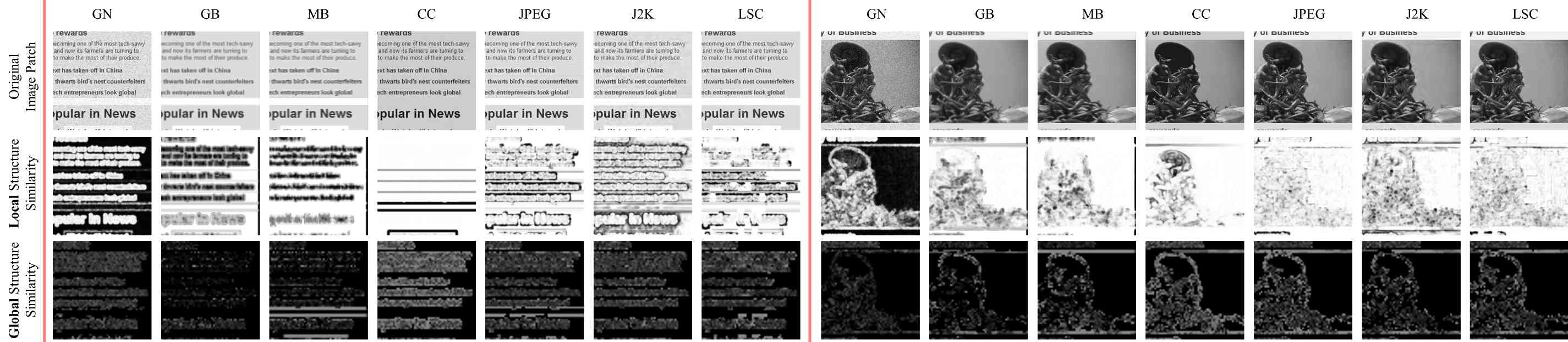
Figure 5. The revealed low-level feature map demonstration. The left/right parts demonstrate several texture/picture cases. Columns from left to right respectively represent different distortion types, including GN (Gaussian Noise), GB (Gaussian Blur), MB (Motion Blur), CC (Contrast Change), JPEG (JPEG Compression), J2K (JPEG2000 Compression), LSC (Layer-segmentation based Compression). [Row 1]: original image patches; [row 2]: the corresponding Local Structure Similarity; [Row 3]: the corresponding Global Structure Similarity.

5. Selective Deep Fusion

Given a reference SCI and a distorted SCI, we have already obtained the global structure similarity feature map ($\rm GSIM^{+}$) and the local structure similarity feature map (LSIM), and we propose to simultaneously feed these two feature maps into the selective deep fusion network for an optimal complementary fusion status.

5.1. Content-aware Adaptive Mid-level Patch Decomposition

Given an off-the-shelf deep network (i.e., we simply adopt the vanilla VGG-16 in this paper), its input layer can only receive input data with fixed size, e.g., $224\times 224$ for the VGG-16. Thus, the conventional methods frequently resort the “resize” operation either over the entire image or the image patches to enable a valid input, see pictorial demonstrations in Fig. 4-A.

Though much progresses have been made by the previous deep learning based works, the widely adopted “resize” operation (e.g., image-level down-sampling or patch-wise up-sampling) may easily induce additional image distortions, leading to limited quality assessment performance eventually, please refer to the quantitative proofs in Tab. 7. To solve the above mentioned problem, here, we advocate a novel mid-level patch decomposition strategy, and its method pipeline can be found in Fig. 4-B. Our novel strategy is capable of conserving both the local and global spatial information (ensured by using a large patch number $n$, see proofs in Tab. 9), yet it can avoid the resizing operation induced patch distortions.

Table 1. Performance comparisons (via 80%-20% training-testing partition) of the deep learning based SOTA SCI quality assessment models on the SIQAD and the SCID datasets. The column-wise bests are marked by bold font. The “-” denotes the absent data.

	SIQAD Dataset								SCID Dataset
Distortion	GN	GB	MB	CC	JPEG	J2K	LSC	Overall	GN	GB	MB	CC	JPEG	J2K	HEV.	CQD	Overall
	PLCC								PLCC
CNN-SQE18 (Zhang et al., 2018)	-	-	-	-	-	-	-	0.904	-	-	-	-	-	-	-	-	0.915
QODCNN-FR19 (Jiang et al., 2019b)	0.918	0.934	0.907	0.866	0.848	0.857	0.897	0.914	-	-	-	-	-	-	-	-	-
RIQA19 (Jianga et al., 2019)	0.920	0.930	0.905	0.857	0.872	0.891	0.857	0.911	-	-	-	-	-	-	-	-	-
SIQA-DF-II19 (Jiang et al., 2019a)	0.912	0.924	0.890	0.844	0.829	0.828	0.858	0.900	-	-	-	-	-	-	-	-	-
SR-CNN	0.916	0.935	0.912	0.852	0.866	0.872	0.875	0.916	0.967	0.938	0.938	0.877	0.963	0.961	0.918	0.922	0.939
	SROCC								SROCC
CNN-SQE18 (Zhang et al., 2018)	0.893	0.924	0.904	0.665	0.847	0.862	0.887	0.894	0.949	0.907	0.878	0.745	0.947	0.939	0.898	0.904	0.914
QODCNN-FR19 (Jiang et al., 2019b)	0.907	0.921	0.895	0.778	0.829	0.835	0.898	0.907	-	-	-	-	-	-	-	-	-
RIQA19 (Jianga et al., 2019)	0.901	0.936	0.893	0.714	0.859	0.890	0.883	0.900	-	-	-	-	-	-	-	-	-
SIQA-DF-II19 (Jiang et al., 2019a)	0.901	0.910	0.880	0.728	0.812	0.816	0.858	0.888	-	-	-	-	-	-	-	-	-
SR-CNN	0.896	0.928	0.910	0.748	0.860	0.874	0.875	0.908	0.957	0.935	0.924	0.810	0.957	0.940	0.885	0.896	0.940
	RMSE								RMSE
CNN-SQE18 (Zhang et al., 2018)	-	-	-	-	-	-	-	6.115	-	-	-	-	-	-	-	-	5.761
QODCNN-FR19 (Jiang et al., 2019b)	5.963	5.454	5.251	6.381	5.141	5.286	3.857	5.801	-	-	-	-	-	-	-	-	-
RIQA19 (Jianga et al., 2019)	6.172	5.712	5.283	6.617	4.767	4.597	4.476	5.880	-	-	-	-	-	-	-	-	-
SIQA-DF-II19 (Jiang et al., 2019a)	6.115	5.768	5.791	6.747	5.840	5.812	4.462	6.242	-	-	-	-	-	-	-	-	-
SR-CNN	5.733	5.089	5.131	6.205	4.496	4.856	3.915	5.683	3.127	3.558	3.679	4.152	3.966	4.225	5.249	4.856	4.830

To be specific, we adaptively select multiple mid-level patches with fixed size $m$ (e.g., $m=224$ for the VGG-16 network), and then feed these mid-level patches related feature maps (i.e., $\rm GSIM^{+}$ and LSIM) to the deep selective fusion network. Specially, we have assigned an identical score (i.e., image-level objective score)for each of these mid-level patches due to the following two aspects:
1) We have adopted a relatively large patch size, i.e., $224\times 224$, and such size is much larger than the common-thread small-size patch-wise partitions (e.g., $11\times 11$), which we believe our patch-wise partition should be categorized as a non-local manner, and thus it may be reasonable to use image-level scores directly;
2) Instead of using RGB patches as input, our mid-level patch-wise partition is performed on the feature maps (i.e., LSIM and $\rm GSIM^{+}$), in which the $\rm GSIM^{+}$ can provide substantial global information even in the case of using such patch-wise formulation.
Due to the different intrinsic attributes for content types, the deep fusion process itself should also treat these patches discriminatively. Thus, given a reference SCI, we conduct K-means clustering using HOG (i.e., $8\times 8$ overlapped tiny patches) respectively over the texture regions ($\textbf{I}^{r}_{t}$) and the picture regions ($\textbf{I}^{r}_{p}$). Hence, it is intuitive to use the cluster center to coarsely locate our mid-level image patches, which can be formulated by Eq. 14.

(14) $$(\xi_{x_{i}},\xi_{y_{i}})\leftarrow({\rm max}\{\xi_{x_{i}},\lfloor\frac{m-1}{2}\rfloor\},{\rm max}\{\xi_{y_{i}},\lfloor\frac{m-1}{2}\rfloor\}),$$

where $\xi_{x_{i}}$ and $\xi_{y_{i}}$ respectively denote the cluster center coordinates ($x$-Horizontal, $y$-Vertical) of the $i$-th clustering, $\lfloor\cdot\rfloor$ denotes the floor operation.

Also, it is worthy mentioning that we choose to use the HOG for clustering due to the following three reasons:
1) In general, there frequently exists remarkable differences in appearance between texture and picture regions, however, it may be more easily to notice such differences from the gradient perspective, i.e., the gradient patterns in texture regions are frequently more regular than those in picture regions;
2) The HOG feature has a strong capability of representing gradient patterns with a relatively low computational cost. In our implementation, we have conducted the HOG feature based clustering in the reference image;
3) Those texture/picture regions frequently share similar HOG patterns if these regions are similar in non-local appearances, ensuring the HOG based clustering centers can be scattered with low overlapping rate. Meanwhile, it should be noted that we utilize the commonly used padding strategy to handle the cases (less than 5% in our adopted datasets) that the SCI image size is smaller than the fixed mid-level patch size. After $2\times n$ mid-level decomposition (i.e., $n$ texture patches and $n$ picture patches), we formulate these mid-level patches into $2\times n$ input data for a single SCI (channel=2), which will be further detailed in the next section.

5.2. Quality Score Regression

So far, we have sparsely represented the input SCI into multiple texture/picture patches with fixed size. Since we aim to achieve an optimal complementary status between the LSIM and the $\rm GSIM^{+}$, for each mid-level patch, we propose to feed its LSIM and $\rm GSIM^{+}$ into the pre-trained deep network to compute deep feature as Eq. 15.

(15) $$\rm{SFeat}\in\mathbb{R}^{1\times 4096}=\rm{FNet}(\rm{LSIM}\oplus\rm{GSIM^{+}}),$$

where the FNet denotes the deep feature computation subnet (i.e., we use the off-the-shelf VGG-16 (Simonyan and Zisserman, 2015)), and its input is $224\times 224\times 2$, where $\oplus$ denotes the feature concatenation operation.

By using Eq. 15, we obtain 4096 dimension deep feature, and then feed it into the regression subnet (RNet), which consists of 2 full connected layers, using typical Euclidean loss. Also, as we have mentioned before that the textual and pictorial regions in the SCIs have different properties, we should train two regression subnets respectively, i.e., one for the textual patches ($\rm RNet_{\emph{t}}$), and another for the picture patches ($\rm RNet_{\emph{p}}$), and the overall network architecture can be found in the right part of Fig. 2. After network training, we formulate the overall quality assessment (FS) as Eq. 16.

(16) $$\rm FS=\frac{0.5}{\emph{n}}\sum_{\emph{i}=1}^{\emph{n}}\rm RNet_{\emph{t}}\{SFeat_{\emph{t}}(\emph{i})\}+\frac{0.5}{\emph{n}}\sum_{\emph{i}=1}^{\emph{n}}RNet_{\emph{p}}\{SFeat_{\emph{p}}(\emph{i})\},$$

where the meaning of $n$ is identical to Sec. 5.1, and its ablation study can be found in Tab. 9.

Meanwhile, because FS (Eq. 16) is mainly derived from the gradient based structure similarity, it it intuitive to use the pixel-wise texture difference to benefit our method, thus we further use the multiplicative based fusion to integrate the Gabor filter based texture similarity (Ni et al., 2018) into our estimated quality score to robust its performance as Eq. 17.

(17) $$\rm FS\leftarrow FS\cdot GF,$$

where GF is the off-the-shelf texture similarity degree provided by the work (Ni et al., 2018).

We implement our model using Matlab R2016a with Caffe (Jia et al., 2014) on a machine with NVIDIA GTX 1080Ti GPU, Intel Xeon W-2133 CPU and 32G RAM. The stochastic gradient descent (SGD) is used to optimise the network with an initial learning rate of $10^{\begin{subarray}{c}-\end{subarray}5}$. The weight decay is $0.0005$, and the momentum is $0.9$. Our network is pre-trained on ImageNet (Deng et al., 2009). During testing, the average predicted scores of $2\times(n-1)$ patches (we have removed the largest and lowest scores empirically) as the final whole-image quality score, and we use “SR-CNN” to denote our method.

Table 2. Cross-dataset quantitative comparisons of our proposed model and other SOTA methods on SIQAD dataset. The row-wise bests are marked with red color, the 2nd-bests are marked with blue color, and the 3rd-bests are marked with black bold font. The “-” denotes the absent data.

	Distortion	PieAPP (Prashnani et al., 2018)	SFUW (Fang et al., 2017)	ESIM (Ni et al., 2017)	CNN-SQE (Zhang et al., 2018)	SVQI (Gu et al., 2017a)	GFM (Ni et al., 2018)	MDOGS (Fu et al., 2018)	EFGD (Wang et al., 2019)	HRFF (Zheng et al., 2019)	QODCNN-FR (Jiang et al., 2019b)	RIQA (Jianga et al., 2019)	SIQA-DF-II (Jiang et al., 2019a)	SR-CNN
		2018	2017	2017	2018	2018	2018	2018	2019	2019	2019	2019	2019
PLCC	GN	0.898	0.887	0.889	-	0.903	0.899	0.898	0.876	0.902	-	0.915	-	0.922
	GB	0.840	0.923	0.923	-	0.913	0.914	0.920	0.932	0.890	-	0.932	-	0.948
	MB	0.788	0.878	0.889	-	0.872	0.866	0.842	0.912	0.874	-	0.869	-	0.936
	CC	0.766	0.829	0.764	-	0.809	0.811	0.801	0.824	0.826	-	0.741	-	0.845
	JPEG	0.735	0.757	0.800	-	0.795	0.840	0.789	0.847	0.763	-	0.871	-	0.854
	J2K	0.843	0.815	0.789	-	0.834	0.849	0.861	0.826	0.754	-	0.834	-	0.893
	Overall	0.757	0.891	0.879	0.904	0.891	0.883	0.884	0.899	0.852	-	0.888	-	0.912
SROCC	GN	0.880	0.869	0.876	0.893	0.891	0.880	0.888	0.867	0.872	-	0.909	-	0.901
	GB	0.840	0.917	0.924	0.924	0.913	0.913	0.919	0.937	0.863	-	0.927	-	0.934
	MB	0.794	0.874	0.894	0.904	0.875	0.870	0.935	0.913	0.850	-	0.872	-	0.932
	CC	0.687	0.722	0.611	0.665	0.713	0.704	0.664	0.762	0.687	-	0.526	-	0.729
	JPEG	0.737	0.750	0.799	0.847	0.793	0.843	0.786	0.846	0.718	-	0.870	-	0.837
	J2K	0.834	0.812	0.783	0.862	0.828	0.844	0.862	0.816	0.744	-	0.860	-	0.899
	Overall	0.742	0.880	0.863	0.894	0.884	0.874	0.882	0.890	0.832	-	0.877	-	0.906
RMSE	GN	6.566	6.876	6.827	-	6.404	6.684	6.558	7.202	6.268	-	5.891	-	5.570
	GB	8.236	5.592	5.827	-	6.155	6.146	5.964	5.519	6.738	-	6.059	-	4.562
	MB	8.006	6.236	5.964	-	6.360	6.518	7.012	5.335	6.466	-	6.327	-	4.447
	CC	8.088	7.048	8.114	-	7.400	7.364	7.528	7.132	6.874	-	8.143	-	6.367
	JPEG	6.372	6.143	5.640	-	5.697	5.101	5.779	4.994	5.862	-	4.509	-	4.571
	J2K	5.589	6.023	6.388	-	5.731	5.499	5.293	5.864	6.501	-	6.127	-	4.369
	Overall	9.352	6.499	6.831	6.115	6.503	6.723	6.695	6.260	7.415	-	6.778	-	5.934

Table 3. Continued cross-dataset quantitative comparisons under different distortion types on the SCID dataset.

	Distortion	PieAPP (Prashnani et al., 2018)	SQMS (Gu et al., 2016)	GSS (Ni et al., 2016a)	SFUW (Fang et al., 2017)	ESIM (Ni et al., 2017)	CNN-SQE (Zhang et al., 2018)	SVQI (Gu et al., 2017a)	GFM (Ni et al., 2018)	EFGD (Wang et al., 2019)	QODCNN-FR (Jiang et al., 2019b)	RIQA (Jianga et al., 2019)	SIQA-DF-II (Jiang et al., 2019a)	SR-CNN
		2018	2016	2016	2017	2017	2018	2018	2018	2019	2019	2019	2019
PLCC	GN	0.898	0.930	0.794	-	0.956	-	0.936	0.950	0.949	0.960	-	-	0.960
	GB	0.874	0.908	0.887	-	0.870	-	0.913	0.916	0.909	0.866	-	-	0.938
	MB	0.787	0.897	0.888	-	0.882	-	0.900	0.902	0.894	0.849	-	-	0.921
	CC	0.749	0.844	0.627	-	0.791	-	0.827	0.879	0.858	0.817	-	-	0.890
	JPEG	0.770	0.930	0.886	-	0.942	-	0.936	0.939	0.949	0.942	-	-	0.958
	J2K	0.843	0.947	0.849	-	0.946	-	0.951	0.923	0.945	0.940	-	-	0.959
	Overall	0.803	0.856	0.774	0.859	0.863	0.915	0.860	0.876	0.885	0.882	-	0.851	0.917
SROCC	GN	0.880	0.916	0.697	0.929	0.946	0.949	0.919	0.937	0.940	0.938	-	-	0.950
	GB	0.846	0.908	0.887	0.897	0.870	0.907	0.908	0.908	0.905	0.856	-	-	0.938
	MB	0.783	0.881	0.873	0.812	0.861	0.878	0.884	0.889	0.869	0.828	-	-	0.898
	CC	0.735	0.803	0.578	0.744	0.618	0.745	0.771	0.823	0.784	0.687	-	-	0.824
	JPEG	0.707	0.924	0.884	0.900	0.946	0.947	0.929	0.928	0.944	0.935	-	-	0.951
	J2K	0.835	0.932	0.836	0.910	0.936	0.939	0.937	0.909	0.933	0.916	-	-	0.942
	Overall	0.787	0.832	0.775	0.856	0.848	0.914	0.839	0.876	0.877	0.876	-	0.851	0.915
RMSE	GN	6.566	4.625	7.647	-	3.676	-	4.418	3.938	3.963	-	-	-	3.430
	GB	6.119	4.434	4.888	-	5.221	-	4.319	4.257	4.419	-	-	-	3.597
	MB	6.530	4.835	5.035	-	5.143	-	4.771	4.612	4.905	-	-	-	4.177
	CC	7.248	4.800	6.976	-	5.479	-	5.037	4.273	4.599	-	-	-	4.005
	JPEG	5.710	5.518	6.984	-	5.037	-	5.305	5.201	4.727	-	-	-	4.195
	J2K	8.084	5.119	8.398	-	5.170	-	4.906	6.139	5.220	-	-	-	4.313
	Overall	5.661	7.328	8.116	-	7.155	-	7.218	6.831	6.604	-	-	7.069	5.284

6. Experimental results

We have evaluated our method over 2 widely adopted datasets, including our previously published SIQAD (Yang et al., 2015) dataset, and SCID (Ni et al., 2017) dataset.

SIQAD Dataset: It contains 20 reference SCIs with diverse visual content and 980 distorted versions generated from the reference SCIs with seven types of image distortions at seven distortion levels, including Gaussian Noise (GN), Gaussian Blur (GB), Motion Blur (MB), Contrast Change (CC), JPEG Compression (JPEG), JPEG2000 Compression (J2K), and the Layer-segmentation based Compression (LSC). The more details about this dataset can be referred to our previous work (Yang et al., 2015).
SCID Dataset: It consists of 40 original SCIs and 1,800 distorted SCIs created with nine different distortion types at five different levels of degradations. The nine distortion types considered are the Gaussian Noise (GN), Gaussian Blur (GB), Motion Blur (MB), Contrast Change (CC), Color Saturation Change (CSC), Color Quantization with Dithering (CQD), JPEG Compression (JPEG), JPEG2000 Compression (J2K), and HEVC Screen Content Compression (HEVC-SCC). The resolution of all SCIs in this dataset is $1280\times 720$.
In the SCID dataset, considering no visual distortion is introduced when the images are viewed in grayscale with the distortion of color saturation change. Thus, we exclude CSC distortion in our work. Also, we have adopted 3 widely adopted evaluation metrics, including PLCC, SROCC and RMSE, and more details can be found in our previous work (Yang et al., 2015).

6.1. Evaluation Metrics

The predicted quality scores by different IQA methods might be nonlinearly related to the subjective scores (i.e., MOS: Mean Opinion Score or DMOS: Differential Mean Opinion Score), we employ a five-parameter logistic transform function to map the quality scores to the MOS/DMOS values as follow.

(18) $$f(x)=\beta_{1}\cdot(\frac{1}{2}-\frac{1}{1+e^{(\beta_{2}\cdot(x-\beta_{3}))}})+\beta_{4}\cdot x+\beta_{5}$$

where $\beta_{1}$, $\beta_{2}$, $\beta_{3}$, $\beta_{4}$ and $\beta_{5}$ are parameters determined by objective scores and subjective scores, and more details can be found in our previous work (Yang et al., 2015).
After the above-mentioned non-linear regression, 3 widely adopted performance criteria are used to evaluate the proposed SR-CNN model and other quality assessment methods: i.e., Pearson Linear Correlation Coefficient (PLCC), Spearman Rank-order Correlation Coefficient (SROCC), and Root Mean Squared Error (RMSE). The PLCC is defined as:

(19) $${\rm PLCC}=\frac{\sum_{\begin{subarray}{c}i\end{subarray}=1}^{N}(O_{i}-\bar{O})(S_{i}-\bar{S})}{\sqrt{\sum_{\begin{subarray}{c}i\end{subarray}=1}^{N}(O_{i}-\bar{O})\cdot\sum_{\begin{subarray}{c}i\end{subarray}=1}^{N}(S_{i}-\bar{S})}}$$

where $O_{i}$ and $S_{i}$ are the objective and subjective scores of the i-th image separately in the database, $\bar{O}$ and $\bar{S}$ are the corresponding mean values of $O_{i}$ and $S_{i}$, $N$ denotes the total number of the images in the dataset.
We can calculate the SROCC as following:

(20) $${\rm SROCC}=1-\frac{6\sum_{\begin{subarray}{c}i\end{subarray}=1}^{N}d_{i}^{2}}{N(N^{2}-1)}$$

where $d_{i}$ is the difference between the i-th image’s rank in the subjective and objective result, respectively.
The RMSE can be computed as following:

(21) $${\rm RMSE}=\sqrt{\frac{\sum_{\begin{subarray}{c}i\end{subarray}=1}^{N}(O_{i}-S_{i})^{2}}{N}}$$

For a superior correlation between the objective and the subjective scores, PLCC=SROCC=1, and RMSE=0. Thus, the higher the values of the PLCC, SROCC and the lower RMSE value, the better the performance of the quality assessment metric.

6.2. Quantitative Comparisons

To demonstrate the performance superiority, we firstly compare the proposed SR-CNN with 4 deep learning based SOTA IQA methods for SCIs, including CNN-SQE18 (Zhang et al., 2018), QODCNN-FR19 (Jiang et al., 2019b), RIQA19 (Jianga et al., 2019) and SIQA-DF-II19 (Jiang et al., 2019a).

Since all these deep learning based methods have adopted the supervised training protocol, we randomly divide the adopted dataset into two non-overlapping subsets by reference images: $80\%$ for training and the rest $20\%$ for testing. We have repeated such 80%-20% partition 50 times, and show the overall performance comparisons in Tab. 1, where the top-3 bests are highlighted in red, blue and black bold, respectively. Meanwhile, because the codes of these deep learning based SOTA methods are currently not public available, we refer the quantitative results of these methods from the original papers. In Tab.. 1, our proposed SR-CNN method significantly outperforms all these SOTA methods over the SIQAD dataset in terms of all measurements (i.e., PLCC, SROCC and RMSE). Also, our method is also leading the performance over the SCID dataset (see Tab. 3).

6.3. Cross-Dataset Evaluation

We also use the cross-dataset validations (using the entire SIQAD or SCID as training set) to verify the generalization ability of the proposed learning model, in which we have conducted an extensive cross-dataset comparisons between the proposed method and 12 SOTA methods, including PieAPP (Prashnani et al., 2018), SQMS (Gu et al., 2016), GSS (Ni et al., 2016a), SFUW (Fang et al., 2017), ESIM (Ni et al., 2017), CNN-SQE (Zhang et al., 2018), SVQI (Gu et al., 2017a), GFM (Ni et al., 2018), EFGD (Wang et al., 2019), QODCNN-FR (Jiang et al., 2019b), RIQA (Jianga et al., 2019) and SIQA-DF-II (Jiang et al., 2019a).

Considering that the adopted two datasets contain different distortion types, we only show the evaluation results over 6 common distortion types, including GN, GB, MB, CC, JPEG and J2K. We show the detailed cross-dataset evaluation results in Tab. 2 and Tab. 3, the top three results are highlighted in red, blue, and black respectively, which indicate that our method outperforms all the compared SOTA methods.

Table 4. The cross-dataset result comparison of DL⁺ and SR-CNN on the SIQAD and SCID

	SIQAD Dataset							SCID Dataset
Distortion	GN	GB	MB	CC	JPEG	J2K	Overall	GN	GB	MB	CC	JPEG	J2K	Overall
	PLCC							PLCC
DL+	0.900	0.930	0.909	0.822	0.850	0.880	0.907	0.952	0.936	0.914	0.881	0.951	0.958	0.915
SR-CNN	0.922	0.948	0.936	0.845	0.854	0.893	0.912	0.960	0.938	0.921	0.890	0.958	0.959	0.917
	SROCC							SROCC
DL+	0.891	0.929	0.911	0.735	0.847	0.882	0.904	0.937	0.936	0.880	0.798	0.946	0.938	0.915
SR-CNN	0.901	0.934	0.932	0.729	0.837	0.899	0.906	0.950	0.938	0.898	0.824	0.951	0.942	0.915
	RMSE							RMSE
DL+	6.512	5.574	5.412	7.173	4.954	4.942	6.197	3.746	3.647	4.387	4.163	4.522	4.420	5.333
SR-CNN	5.570	4.562	4.447	6.367	4.571	4.369	5.934	3.430	3.597	4.177	4.005	4.195	4.313	5.284

6.4. Parameter and Component Evaluation

There are many parameters are predefined in our method, including $\alpha_{1}$, $\alpha_{2}$, $\beta_{1}$ and $\beta_{2}$, which were mentioned in $\rm GSIM_{t/p}^{+}$ (Eq. 9) and $\rm FSIM$ (Eq. 13), respectively. So, we resort a extensive ablation study on these parameters to facilitate an optimal choice. We initially fixed $\beta=1$ and simply tested multiple choices of $\alpha_{1}$ (ranging from 0.1 to 0.5) and $\alpha_{2}$ (ranging from 0 to 0.8), and assign $\alpha_{1}=0.2$ and $\alpha_{2}=0.6$ as the optimal choice according to Tab. 5 and Tab. 6.

Table 5. Analysis of GSIM_t/p⁺ result with different $\alpha_{1}$ values on the SIQAD and the SCID

$\beta_{1}$=1	SIQAD			SCID
	PLCC	SROCC	RMSE	PLCC	SROCC	RMSE
$\alpha_{1}$=0.1	0.839	0.827	7.781	0.845	0.844	7.630
$\alpha_{1}$=0.2	0.843	0.827	7.707	0.846	0.843	7.593
$\alpha_{1}$=0.3	0.840	0.820	7.762	0.814	0.811	8.285
$\alpha_{1}$=0.4	0.826	0.796	8.076	0.749	0.737	9.452
$\alpha_{1}$=0.5	0.790	0.738	8.773	0.639	0.621	10.970

Table 6. Analysis of FSIM result with different $\alpha_{2}$ values on the SIQAD and the SCID

$\beta_{2}$=1	SIQAD			SCID
	PLCC	SROCC	RMSE	PLCC	SROCC	RMSE
$\alpha_{2}$=0.0	0.843	0.827	7.707	0.846	0.843	7.593
$\alpha_{2}$=0.2	0.858	0.848	7.352	0.855	0.851	7.392
$\alpha_{2}$=0.4	0.865	0.859	7.188	0.857	0.852	7.351
$\alpha_{2}$=0.6	0.867	0.863	7.130	0.857	0.851	7.345
$\alpha_{2}$=0.8	0.867	0.864	7.146	0.853	0.849	7.432

We further conduct component evaluation to validate the effectiveness of each component adopted in our method. As shown in Tab. 7, the solely local structure similarity (Eq. 10) based measurement (denoted by LSIM) exhibits the worst performance, which is even slightly worse than the solely global structure similarity based measurement (denoted by GSIM). Then, the overall performance can get a significant improvement by dividing the input SCI into texture and picture regions beforehand, which we denote it as $\rm GSIM_{t/p}$. Further, the overall performance can get further enhanced by measuring the structure similarity from the dictionary perspective (Eq. 9), and we denote its performance as $\rm GSIM_{t/p}^{+}$. By using the multiplicative based fusion to integrate the $\rm GSIM_{t/p}^{+}$ into the local structure similarity measurement (Eq. 12), the overall performance get a further improvement, which we denote it as FSIM (Eq. 13). Also, our newly designed selective fusion network is capable of significantly improving the overall performance ($\rm DL$), which simply feeds the “resized” feature maps into CNN based deep network. Specially, our mid-level patch strategy (Sec. 5.1) is able to avoid the “resize” operation induced additional distortions effectively, and we denote its performance by $\rm DL^{+}$. Meanwhile, the integrated off-the-shelf texture similarity (Eq. 17) also benefits our method slightly, and we denote its performance as our complete version, i.e., the SR-CNN, achieving the best performance.

Table 7. The detailed component quantitative evaluation results

Components	SIQAD Dataset			SCID Dataset
	PLCC	SROCC	RMSE	PLCC	SROCC	RMSE
LSIM	0.754	0.759	9.400	0.772	0.750	9.062
GSIM	0.758	0.734	9.329	0.779	0.757	8.984
GSIMt/p	0.834	0.821	7.908	0.842	0.838	7.681
GSIMt/p+	0.843	0.827	7.707	0.846	0.843	7.593
FSIM	0.867	0.863	7.130	0.877	0.872	7.038
DL	0.821	0.806	8.516	0.832	0.818	8.254
DL+	0.912	0.904	5.792	0.936	0.937	4.964
SR_CNN	0.916	0.908	5.683	0.939	0.940	4.830

Moreover, we have also tested the performance of the CNN model which using the RGB information only (without using both LSIM and GSIM features). As shown in Tab. 8, our newly designed hand-crafted features can effectively boost the solely RGB information trained RGB-CNN model significantly, e.g., almost 6% overall PLCC and SROCC over the SCID dataset.

In addition, we also make cross-dataset experiments to compare performances of the $\rm DL^{+}$ and SR-CNN mentioned in Eq. 17. The detailed cross-dataset validation results are shown in Tab. 4, which further verified the effectiveness of our integrated off-the-shelf texture similarity.

Table 8. The quantitative evaluation between the RGB trained CNN model and the proposed SR-CNN on the SIQAD and SCID datasets.

	SIQAD Dataset								SCID Dataset
Distortion	GN	GB	MB	CC	JPEG	J2K	LSC	Overall	GN	GB	MB	CC	JPEG	J2K	HEV.	CQD	Overall
	PLCC								PLCC
RGB-CNN	0.914	0.933	0.885	0.821	0.841	0.766	0.804	0.898	0.959	0.882	0.869	0.824	0.912	0.874	0.838	0.827	0.872
SR-CNN	0.916	0.935	0.912	0.852	0.866	0.872	0.875	0.916	0.967	0.938	0.938	0.877	0.963	0.961	0.918	0.922	0.939
	SROCC								SROCC
RGB-CNN	0.891	0.918	0.883	0.718	0.828	0.755	0.792	0.885	0.950	0.883	0.868	0.656	0.897	0.844	0.750	0.781	0.869
SR-CNN	0.896	0.928	0.910	0.748	0.860	0.874	0.875	0.908	0.957	0.935	0.924	0.810	0.957	0.940	0.885	0.896	0.940
	RMSE								RMSE
RGB-CNN	5.852	5.150	5.664	6.718	4.838	6.107	4.886	6.164	3.460	4.876	5.241	4.958	6.105	7.517	7.585	7.122	6.928
SR-CNN	5.733	5.089	5.131	6.205	4.496	4.856	3.915	5.683	3.127	3.558	3.679	4.152	3.966	4.225	5.249	4.856	4.830

Meanwhile, we have conducted the ablation study to select an optimal patch number ($n$), mentioned in our patch adaptively selection strategy (Sec. 5.1). The ablation results can be found in Tab. 9, which indicate that the parameter $n$ is positively related to the overinsurance. Since the performance improvement tendency is shrinking when $n\geq 6$, we assign $n=6$ as the optimal choice to strike the trade-off between performance and computation.

Table 9. Mid-level patch selection ablation study.

number	0 patches	3 patches	6 patches	9 patches
PLCC	0.821	0.914	0.916	0.914
SROCC	0.806	0.906	0.908	0.907
RMSE	8.516	5.687	5.683	5.692

6.5. Limitation

In addition to the accuracy as discussed above, the computational complexity of the IQA model is another important aspect to be assessed. Here we list the single image computation time comparisons over the SIQAD dataset in Tab. 10. All of these tests are performed by running Matlab R2016a on a desktop computer with i7-6700 3.40GHz CPU, GTX 1080 GPU, 32GB RAM (all the hand-crafted pre-processing stages are conducted on CPU, yet the selective deep fusion is performed on GPU). Actually, our proposed SR-CNN is relatively time-consuming, which is mainly induced by the heavy time computation cost of the adopted OMP re-construction procedure (almost 17s per-image).

Table 10. Runtime comparison (seconds) between 6 most representative methods on the SIQAD dataset.

Model	SFUW17	ESIM17	CNN-SQE18	SVQI18	GFM18	SR-CNN
Time/s	189.680	3.013	37.040	2.432	0.167	26.608

7. Conclusion

In this paper, we have proposed a full reference quality assessment method for SCIs. The proposed method includes two main stages: 1) The structure-aware SCI quality assessment stage; 2) The selective deep fusion stage. At the first stage, we propose to use the sparse representation to aid a novel global structure similarity (GSIM) measurement. The conventional local metric is also adopted to improve its robustness. Then, at the second stage, we adopt the newly-designed selective deep fusion network to fuse multi-level structure similarity measurement, achieving an optimal complementary status. We have conducted extensive quantitative evaluations to demonstrate the efficacy and effectiveness of our method. Our method is simple yet effective with a clear motivation, continuing to improve the current SOTA methods and techniques with new features and advantages.

- (1)
- Aharon et al. (2006) Michal Aharon, Michael Elad, and Alfred Bruckstein. 2006. K-SVD: An algorithm for designing overcomplete dictionaries for sparse representation. IEEE Transactions on signal processing 54, 11 (2006), 4311–4322.
- Chang et al. (2014) Tsuishan Chang, Chunchi Chen, Ruling Liao, Chewei Kuo, and Wenhsiao Peng. 2014. Intra line copy for HEVC screen content coding. In Asia-pacific Signal & Information Processing Association, Summit & Conference. 1–8.
- Chen et al. (2016a) Chenglizhao Chen, Shuai Li, and Hong Qin. 2016a. Robust Salient Motion Detection in Non-stationary Videos via Novel Integrated Strategies of Spatio-temporal Coherency Clues and Low-rank Analysis. Pattern Recognition 52 (2016), 410–432.
- Chen et al. (2015a) Chenglizhao Chen, Shuai Li, Hong Qin, and Aimin Hao. 2015a. Real-time and robust object tracking in video via low-rank coherency analysis in feature space. Pattern Recognition 48, 9 (2015), 2885–2905.
- Chen et al. (2015b) Chenglizhao Chen, Shuai Li, Hong Qin, and Aimin Hao. 2015b. Structure-Sensitive Saliency Detection via Multilevel Rank Analysis in Intrinsic Feature Space. IEEE Transactions on Image Processing 24, 8 (2015), 2303–2316.
- Chen et al. (2016b) Chenglizhao Chen, Shuai Li, Hong Qin, and Aimin Hao. 2016b. Robust salient motion detection in non-stationary videos via novel integrated strategies of spatio-temporal coherency clues and low-rank analysis. Pattern Recognition 52 (2016), 410–432.
- Chen et al. (2018b) Chenglizhao Chen, Shuai Li, Hong Qin, Zhenkuan Pan, and Guowei Yang. 2018b. Bi-level Feature Learning for Video Saliency Detection. IEEE Transactions on Multimedia (2018).
- Chen et al. (2017) Chenglizhao Chen, Shuai Li, Yongguang Wang, Hong Qin, and Aimin Hao. 2017. Video saliency detection via spatial-temporal fusion and low-rank coherency diffusion. IEEE Transactions on Image Processing 26, 7 (2017), 3156–3170.
- Chen et al. (2018a) Chenglizhao Chen, Yunxiao Li, Shuai Li, Hong Qin, and Aimin Hao. 2018a. A novel bottom-up saliency detection method for video with dynamic background. IEEE Signal Processing Letters 25, 2 (2018), 154–158.
- Chen et al. (2019) Chenglizhao Chen, Guotao Wang, Chong Peng, Xiaowei Zhang, and Hong Qin. 2019. Improved Robust Video Saliency Detection based on Long-term Spatial-temporal Information. IEEE Trans. on Image Process. (TIP) 29 (2019), 1090–1100.
- Chen et al. (2020) Chenglizhao Chen, Jipeng Wei, Chong Peng, Weizhong Zhang, and Hong Qin. 2020. Improved Saliency Detection in RGB-D Images using Two-phase Depth Estimation and Selective Deep Fusion. IEEE Trans. on Image Process. (TIP) 29 (2020), 4296–4307.
- Chen et al. (2018c) Jianan Chen, Liquan Shen, Linru Zheng, and Xuhao Jiang. 2018c. Naturalization Module in Neural Networks for Screen Content Image Quality Assessment. IEEE Signal Processing Letters 25, 11 (2018), 1685–1689.
- Cheng et al. (2018) Zhengxue Cheng, Masaru Takeuchi, Kenji Kanai, and Jiro Katto. 2018. A Fast No-Reference Screen Content Image Quality Prediction Using Convolutional Neural Networks. In IEEE International Conference on Multimedia & Expo Workshops. 1–6.
- Deng et al. (2009) Jia Deng, Wei Dong, Richard Socher, Lijia Li, Kai Li, and Feifei Li. 2009. ImageNet: a Large-Scale Hierarchical Image Database. In IEEE Conference on Computer Vision and Pattern Recognition. 248–255.
- Fang et al. (2018) Yuming Fang, Jiebin Yan, Leida Li, Jinjian Wu, and Weisi Lin. 2018. No Reference Quality Assessment for Screen Content Images With Both Local and Global Feature Representation. IEEE Transactions on Image Processing 27, 4 (2018), 1600–1610.
- Fang et al. (2017) Yuming Fang, Jiebin Yan, Jiaying Liu, Shiqi Wang, Qiaohong Li, and Zongming Guo. 2017. Objective Quality Assessment of Screen Content Images by Uncertainty Weighting. IEEE Transactions on Image Processing 26, 4 (2017), 2016–2027.
- Freitas et al. (2018) Pedro Garcia Freitas, Sana Alamgeer, Welington Y. L. Akamine, and Mylène C. Q. Farias. 2018. Blind Image Quality Assessment Based on Multiscale Salient Local Binary Patterns. In Proceedings of the 9th ACM Multimedia Systems Conference. Association for Computing Machinery, 52–63.
- Fu et al. (2018) Ying Fu, Huanqiang Zeng, Lin Ma, Zhangkai Ni, Jianqing Zhu, and Kaikuang Ma. 2018. Screen content image quality assessment using multi-scale difference of gaussian. IEEE Transactions on Circuits and Systems for Video Technology 28, 9 (2018), 2428–2432.
- Gu et al. (2017a) Ke Gu, Junfei Qiao, Xiongkuo Min, Guanghui Yue, Weisi Lin, and Daniel Thalmann. 2017a. Evaluating Quality of Screen Content Images Via Structural Variation Analysis. IEEE Transactions on Visualization and Computer Graphics 24, 10 (2017), 2689–2701.
- Gu et al. (2016) Ke Gu, Shiqi Wang, Huan Yang, Weisi Lin, Guangtao Zhai, Xiaokang Yang, and Wenjun Zhang. 2016. Saliency-Guided Quality Assessment of Screen Content Images. IEEE Transactions on Multimedia 18, 6 (2016), 1098–1110.
- Gu et al. (2015) Ke Gu, Shie Wang, Gaohong Zhai, Siwei Ma, and Weisi Lin. 2015. Screen image quality assessment incorporating structural degradation measurement. In IEEE International Symposium on Circuits and Systems. 125–128.
- Gu et al. (2017b) Ke Gu, Jun Zhou, Junfei Qiao, Guangtao Zhai, Weisi Lin, and Alan Bovik. 2017b. No-Reference Quality Assessment of Screen Content Pictures. IEEE Transactions on Image Processing 26, 8 (2017), 4005–4018.
- Hu et al. (2014) Han Hu, Yonggang Wen, Huanbo Luan, Tat-Seng Chua, and Xuelong Li. 2014. Toward Multiscreen Social TV with Geolocation-Aware Social Sense. IEEE Multimedia 21, 3 (2014), 10–19.
- Jaderberg et al. (2014) Max Jaderberg, Andrea Vedaldi, and Andrew Zisserman. 2014. Deep Features for Text Spotting. In European Conference on Computer Vision. 512–528.
- Jia et al. (2014) Yangqing Jia, Evan Shelhamer, Jeff Donahue, Sergey Karayev, Jonathan Long, Ross Girshick, Sergio Guadarrama, and Trevor Darrell. 2014. Caffe: Convolutional Architecture for Fast Feature Embedding. In Proceedings of the 22Nd ACM International Conference on Multimedia. 675–678.
- Jiang et al. (2019a) Xuhao Jiang, Liquan Shen, Qing Ding, Linru Zheng, and Ping An. 2019a. Screen content image quality assessment based on convolutional neural networks. Journal of Visual Communication and Image Representation 67 (2019), 27–45.
- Jiang et al. (2019b) Xuhao Jiang, Liquan Shen, Guorui Feng, Liangwei Yu, and Ping An. 2019b. Deep Optimization model for Screen Content Image Quality Assessment using Neural Networks. CoRR (2019).
- Jianga et al. (2019) Xuhao Jianga, Liquan Shen, Liangwei Yu, Mingxing Jiang, and Guorui Feng. 2019. No-reference screen content image quality assessment based on multi-region features. Neurocomputing 52 (2019), 410–432.
- Li et al. (2019) Yunxiao Li, Shuai Li, Chenglizhao Chen, Hong Qin, and Aimin Hao. 2019. Accurate and Robust Video Saliency Detection via Selfpaced Diffusion. IEEE Trans. on Multimedia (TMM) (2019), early access.
- Liu et al. (2012) Anmin Liu, Weisi Lin, and Manish Narwaria. 2012. Image quality assessment based on gradient similarity. IEEE Transactions on Image Processing 21, 4 (2012), 1500–1512.
- Ma et al. (2019) Guangxiao Ma, Chenglizhao Chen, Shuai Li, Chong Peng, Aimin Hao, and Hong Qin. 2019. Salient Object Detection via Multiple Instance Joint Re-learning. IEEE Trans. on Multimedia (TMM) (2019).
- Ma et al. (2014) Zhan Ma, Wei Wang, Meng Xu, and Haoping Yu. 2014. Advanced screen content coding using color table and index map. IEEE Transactions on Image Processing 23, 10 (2014), 4399–4412.
- Miao et al. (2016) Dan Miao, Jingjing Fu, Yan Lu, Shipeng Li, and ChangWen Chen. 2016. A High-Fidelity and Low-Interaction-Delay Screen Sharing System. ACM Transactions on Multimedia Computing, Communications, and Applications 12, 3 (2016), 1–23.
- Min et al. (2017) Xiongkuo Min, Kede Ma, Ke Gu, Guangtao Zhai, Zhou Wang, and Weisi Lin. 2017. Unified Blind Quality Assessment of Compressed Natural, Graphic and Screen Content Images. IEEE Transactions on Image Processing 26, 11 (2017), 5462–5474.
- Ni et al. (2016a) Zhangkai Ni, Lin Ma, Huanqiang Zeng, Canhui Cai, and Kk. Ma. 2016a. Gradient Direction for Screen Content Image Quality Assessment. IEEE Signal Processing Letters 23, 10 (2016), 1394–1398.
- Ni et al. (2016b) Zhangkai Ni, Lin Ma, Huanqiang Zeng, Canhui Cai, and Kaikuang Ma. 2016b. Screen content image quality assessment using edge model. In IEEE International Conference on Image Processing. 81–85.
- Ni et al. (2017) Zhangkai Ni, Lin Ma, Huanqiang Zeng, Jing Chen, Canhui Cai, and Kai-Kuang Ma. 2017. ESIM: Edge Similarity for Screen Content Image Quality Assessment. IEEE Transactions on Image Processing 26, 10 (2017), 4818–4831.
- Ni et al. (2018) Zhangkai Ni, Huanqiang Zeng, Lin Ma, Junhui Hou, Jing Chen, and Kai-Kuang Ma. 2018. A Gabor Feature-Based Quality Assessment Model for the Screen Content Images. IEEE Transactions on Image Processing 27, 9 (2018), 4516–4528.
- Pati et al. (1993) Yagyenshchandra Pati, Ramin Rezaiifar, and Perinkulamsambamurthy Krishnaprasad. 1993. Orthogonal matching pursuit: Recursive function approximation with applications to wavelet decomposition. In Proceedings of 27th Asilomar Conference on Signals, Systems and Computers. 40–44.
- Peng et al. (2020) Chong Peng, Chenglizhao Chen, Zhao Kang, and Qiang Cheng. 2020. Robust Principal Component Analysis: A Factorization Based Approach with Linear Complexity. Information Sciences 513 (2020), 581–599.
- Peng et al. (2019) Chong Peng, Chenglizhao Chen, Zhao Kang, Jianbo Li, and Qiang Cheng. 2019. RES-PCA: A Scalable Approach to Recovering Low-rank Matrices. In Proc. IEEE Conf. Comput. Vis. Pattern Recognit. (CVPR).
- Prashnani et al. (2018) Ekta Prashnani, Hong Cai, Yasamin Mostofi, and Pradeep Sen. 2018. PieAPP: Perceptual Image-Error Assessment through Pairwise Preference. In IEEE Conference on Computer Vision and Pattern Recognition. 1808–1817.
- Qian et al. (2017) Jiansheng Qian, Lijuan Tang, Vinit Jakhetiya, Zhifang Xia, Ke Gu, and Hong Lu. 2017. Towards efficient blind quality evaluation of screen content images based on edge-preserving filter. Electronics Letters 53, 9 (2017), 592–594.
- Simonyan and Zisserman (2015) Karen Simonyan and Andrew Zisserman. 2015. Very Deep Convolutional Networks for Large-Scale Image Recognition. In International Conference on Learning Representations.
- Wang et al. (2019) Ruifeng Wang, Huan Yang, Zhenkuan Pan, Baoxiang Huang, and Guoji Hou. 2019. Screen Content Image Quality Assessment With Edge Features in Gradient Domain. IEEE Access 7 (2019), 5285–5295.
- Wang et al. (2015) Shiqi Wang, Ke Gu, Kai Zeng, Zhou Wang, and Weisi Lin. 2015. Perceptual screen content image quality assessment and compression. In IEEE International Conference on Image Processing. 1434–1438.
- Wang et al. (2016) Shiqi Wang, Ke Gu, Kai Zeng, Zhou Wang, and Weisi Lin. 2016. Objective Quality Assessment and Perceptual Compression of Screen Content Images. IEEE Computer Graphics and Applications 38, 1 (2016), 47–58.
- Wang et al. (2004) Zhou Wang, Alanconrad Bovik, Hamidrahim Sheikh, and Eerop Simoncelli. 2004. Image quality assessment: from error visibility to structural similarity. IEEE Transactions on Image Processing 13, 4 (2004), 600–612.
- Wang and Li (2011) Zhou Wang and Qiang Li. 2011. Information content weighting for perceptual image quality assessment. IEEE Transactions on Image Processing 20, 5 (2011), 1185–1198.
- Wang and Shang (2006) Zhou Wang and Xinli Shang. 2006. Spatial Pooling Strategies for Perceptual Image Quality Assessment. In IEEE International Conference on Image Processing. 2945–2948.
- Xing et al. (2017) Lu Xing, Lei Cai, Huanqiang Zeng, Jing Chen, Jianqing Zhu, and Junhui Hou. 2017. A Multi-scale Contrast-based Image Quality Assessment Model for Multi-Exposure Image Fusion. Signal Processing 145 (2017), 233–240.
- Xue et al. (2014) Wufeng Xue, Lei Zhang, Xuanqin Mou, and Alanc Bovik. 2014. Gradient Magnitude Similarity Deviation: A Highly Efficient Perceptual Image Quality Index. IEEE Transactions on Image Processing 23, 2 (2014), 684–695.
- Yang et al. (2015) Huan Yang, Yuming Fang, and Weisi Lin. 2015. Perceptual Quality Assessment of Screen Content Images. IEEE Transactions on Image Processing 24, 11 (2015), 4408–4421.
- Zhang et al. (2014) Lin Zhang, Ying Shen, and Hongyu Li. 2014. VSI: a visual saliency-induced index for perceptual image quality assessment. IEEE Transactions on Image Processing 23, 10 (2014), 4270–4281.
- Zhang et al. (2013) Xuande Zhang, Xiangchu Feng, Weiwei Wang, and Wufeng Xue. 2013. Edge Strength Similarity for Image Quality Assessment. IEEE Signal Processing Letters 20, 4 (2013), 319–322.
- Zhang et al. (2018) Yi Zhang, Damon Chandler, and Xuanqin Mou. 2018. Quality Assessment of Screen Content Images via Convolutional-Neural-Network-Based Synthetic/Natural Segmentation. IEEE Transactions on Image Processing 27, 10 (2018), 5113–5128.
- Zheng et al. (2019) Linru Zheng, Liquan Shen, Jianan Chen, Ping An, and Jun Luo. 2019. No-Reference Quality Assessment for Screen Content Images Based on Hybrid Region Features Fusion. IEEE Transactions on Multimedia 21, 8 (2019), 2057–2070.
- Zhou et al. (2018) Wujie Zhou, Lu Yu, Yang Zhou, Weiwei Qiu, Mingwei Wu, and Ting Luo. 2018. Local and Global Feature Learning for Blind Quality Evaluation of Screen Content and Natural Scene Images. IEEE Transactions on Image Processing 27, 5 (2018), 2086–2095.
- Zhu et al. (2015) Weijia Zhu, Wenpeng Ding, Jizheng Xu, Yunhui Shi, and Baocai Yin. 2015. Hash Based Block Matching for Screen Content Coding. IEEE Transactions on Multimedia 17, 7 (2015), 935–944.
- Zuo et al. (2016) Lingxuan Zuo, Hanli Wang, and Jie Fu. 2016. Screen content image quality assessment via convolutional neural network. In IEEE International Conference on Image Processing. 2082–2086.