Revisiting Modified Greedy Algorithm for Monotone Submodular Maximization with a Knapsack Constraint

Abstract.

Monotone submodular maximization with a knapsack constraint is NP-hard. Various approximation algorithms have been devised to address this optimization problem. In this paper, we revisit the widely known modified greedy algorithm. First, we show that this algorithm can achieve an approximation factor of $0.405$, which significantly improves the known factors of $0.357$ given by Wolsey [44] and $(1-1/{\mathrm{e}})/2\approx 0.316$ given by Khuller et al. [19]. More importantly, our analysis closes a gap in Khuller et al.’s proof for the extensively mentioned approximation factor of $(1-1/\sqrt{{\mathrm{e}}})\approx 0.393$ in the literature to clarify a long-standing misconception on this issue. Second, we enhance the modified greedy algorithm to derive a data-dependent upper bound on the optimum. We empirically demonstrate the tightness of our upper bound with a real-world application. The bound enables us to obtain a data-dependent ratio typically much higher than $0.405$ between the solution value of the modified greedy algorithm and the optimum. It can also be used to significantly improve the efficiency of algorithms such as branch and bound.

1. Introduction

A set function $f\colon 2^{V}\rightarrow\mathbb{R}$ is submodular [31] if for all $S,T\subseteq V$, it holds that

$$f(S)+f(T)\geq f(S\cup T)+f(S\cap T).$$

Alternatively, defining

$$f(v\mid S):=f(S\cup\{v\})-f(S)$$

as the marginal gain of adding an element $v\in V$ to a set $S\subseteq V$, an equivalent definition of a submodular set function $f$ is that for all $S\subseteq T$ and $v\in V\setminus T$,

$$f(v\mid S)\geq f(v\mid T).$$

The latter form of definition describes the concept of diminishing return in economics. The function $f$ is monotone nondecreasing if and only if $f(S)\leq f(T)$ for all $S\subseteq T$ (or equivalently $f(v\mid S)\geq 0$).

Many well known combinatorial optimization problems are essentially monotone submodular maximization, such as maximum coverage [11, 19], maximum facility location [8, 2], and maximum entropy sampling [33, 20]. In addition, a growing number of problems in real-world applications of artificial intelligence and machine learning are also shown to be monotone submodular maximization. These problems include sensor placement [23, 24], feature selection [21, 46], viral marketing [17, 18], image segmentation [5, 9, 16], document summarization [28, 29], data subset selection [22, 43], etc.

In this paper, we study monotone submodular maximization with a knapsack constraint, which is defined as follows:

(1) $$\max_{S\subseteq V}f(S)\text{ s.t.\@ }c(S)\leq b,$$

where $f$ is a monotone nondecreasing submodular set function, $c(S)=\sum_{v\in S}c(v)$ and $c(v)$ represents the cost of element $v$. Without loss of generality, we may assume that the cost of each element does not exceed $b$, since elements with cost greater than $b$ do not belong to any feasible solution. This optimization problem has already found great utility in the aforementioned applications.

Since this optimization problem is NP-hard in general, various approximation algorithms have been proposed. For a special cardinality constraint where the costs of all elements are identical, i.e., $c(v)=1$ for every element $v\in V$, Nemhauser et al. [31] proposed a simple hill-climbing greedy algorithm that can provide $(1-1/{\mathrm{e}})$-approximation (we say that an algorithm provides $\alpha$-approximation, where $\alpha\leq 1$, if it always obtains a solution of value at least $\alpha$ times the value of an optimal solution). However, for the general knapsack constraint, the approximation factor of such a greedy algorithm is unbounded. Wolsey [44] found that slightly modifying the original greedy algorithm can provide an approximation ratio of $(1-1/{\mathrm{e}}^{\beta})\approx 0.357$, where $\beta$ is the unique root of the equation ${\mathrm{e}}^{x}=2-x$. Khuller et al. [19] studied the budgeted maximum coverage problem (a special case of monotone submodular maximization with a knapsack constraint where the function value is always an integer), and derived two approximation factors, i.e., $(1-1/{{\mathrm{e}}})/2\approx 0.316$ and $(1-1/\sqrt{{\mathrm{e}}})\approx 0.393$, for the modified greedy algorithm developed by Wolsey [44]. We note that the factor of $(1-1/\sqrt{{\mathrm{e}}})$ is extensively mentioned in the literature, but unfortunately their proof was flawed as pointed out by Zhang et al. [47]. It becomes an open question whether the modified greedy algorithm can achieve an approximation ratio at least $(1-1/\sqrt{{\mathrm{e}}})$.

Khuller et al. [19] also developed a partial enumeration greedy algorithm that improves the approximation factor to $(1-1/{\mathrm{e}})$, which was later shown to be applicable to the general problem (1) [34]. However, this algorithm requires $O(n^{5})$ (where $n=\lvert V\rvert$ is the total number of elements in the ground set $V$) function value computations, which is not scalable. We focus on the scalable modified greedy algorithm of $O(n^{2})$ [19] and conduct a comprehensive analysis on its worst-case approximation guarantee. Based on the monotonicity and submodularity, we derive several relations governing the solution value and the optimum. Leveraging these relations, we establish an approximation ratio of $0.405$, which significantly improves the factors of $(1-1/{\mathrm{e}}^{\beta})\approx 0.357$ given by Wolsey [44] and $(1-1/{{\mathrm{e}}})/2\approx 0.316$ given by Khuller et al. [19]. More importantly, our analysis fills a critical gap in the proof for the factor of $(1-1/\sqrt{{\mathrm{e}}})\approx 0.393$ given by Khuller et al. [19] to clarify a long-standing misconception in the literature.

In addition, we enhance the modified greedy algorithm to derive a data-dependent upper bound on the optimum. We empirically demonstrate the tightness of our bound with a real-world application of viral marketing in social networks. The bound enables us to obtain a data-dependent ratio typically much higher than $0.405$ between the solution value of the modified greedy algorithm and the optimum. It can also be used to significantly improve the efficiency of algorithms such as branch and bound as shown by our experimental evaluations.

2. Modified Greedy Algorithm and Approximation Guarantees

For the unit cost version of the optimization problem defined in (1), a simple greedy algorithm that chooses the element with the largest marginal gain in each iteration can achieve an approximation factor of $(1-1/{\mathrm{e}})$ [31]. Inspired by this elegant algorithm, for the general cost version, it is natural to apply a similar greedy algorithm according to cost-effectiveness. That is, we pick in each iteration the element that maximizes the ratio $\frac{f(v\mid S_{\mathrm{g}})}{c(v)}$ based on the selected element set $S_{\mathrm{g}}$. Unfortunately, this simple greedy algorithm has an unbounded approximation factor. Consider, for example, two elements $u$ and $v$ with $f(\{u\})=1$, $f(\{v\})=2\varepsilon$, $c(u)=1$ and $c(v)=\varepsilon$, where $\varepsilon$ is a small positive number. When $b=1$, the optimal solution is $\{u\}$ while the greedy heuristic picks $\{v\}$. The approximation factor for this instance is $2\varepsilon$, and is therefore unbounded.

1 initialize $S_{\mathrm{g}}\leftarrow\emptyset$, $V^{\prime}\leftarrow V$;

2 while $V^{\prime}\neq\emptyset$ do

3       find $u\leftarrow\arg\max_{v\in V^{\prime}}\big{\{}\frac{f(v\mid S_{\mathrm{g}})}{c(v)}\big{\}}$;

4       if $c(S)+c(u)\leq b$ then

5            $S_{\mathrm{g}}\leftarrow S_{\mathrm{g}}\cup\{u\}$;

6            

7      update the search space $V^{\prime}\leftarrow V^{\prime}\setminus\{u\}$;

8      

9$v^{\ast}\leftarrow\arg\max_{v\in V}f(v)$;

10 $S_{\mathrm{m}}\leftarrow\arg\max_{S\in\{\{v^{*}\},S_{\mathrm{g}}\}}f(S)$;

11 return $S_{\mathrm{m}}$;

Algorithm 1 MGreedy

Interestingly, a small modification to the greedy algorithm, referred to as MGreedy (Algorithm 1), achieves a constant approximation factor [19, 44]. Specifically, in addition to $S_{\mathrm{g}}$ obtained from the greedy heuristic (Lines 1–1), the algorithm also finds an element $v^{\ast}$ that maximizes $f(\{v\})$ (Line 1), and then chooses the better one between $S_{\mathrm{g}}$ and $\{v^{\ast}\}$ (Lines 1 and 1). Wolsey [44] showed that MGreedy achieves an approximation factor of $0.357$. Later, Khuller et al. [19] gave two approximation factors of $(1-1/{\mathrm{e}})/2$ and $(1-1/\sqrt{{\mathrm{e}}})$ that can be achieved by MGreedy for the budgeted maximum coverage problem, but unfortunately their proof for the factor of $(1-1/\sqrt{{\mathrm{e}}})$ was flawed as pointed out by Zhang et al. [47]. In Section 6.2, we provide an explanation of the problem in Khuller et al.’s proof and show a correct proof for the factor of $(1-1/\sqrt{{\mathrm{e}}})$. A main result of this paper is to establish an improved approximation factor of $0.405$ for MGreedy.

Theorem 2.1.

Let $\alpha^{\bot}$ be the root of

(2) $$(1-\alpha^{\bot})\ln(1-\alpha^{\bot})+(2-1/{\mathrm{e}})(1-2\alpha^{\bot})=0$$

satisfying $\alpha^{\bot}>0.405$. The MGreedy algorithm achieves an approximation factor of $\alpha^{\bot}$.

To our knowledge, this is the first work giving a constant factor achieved by MGreedy that is even larger than $(1-1/\sqrt{{\mathrm{e}}})\approx 0.393$, which not only significantly improves the known factors of $(1-1/{\mathrm{e}}^{\beta})\approx 0.357$ given by Wolsey [44] and $(1-1/{\mathrm{e}})/2\approx 0.316$ given by Khuller et al. [19] but also clarifies a long-term misunderstanding regarding the factor of $(1-1/\sqrt{{\mathrm{e}}})$ in the literature.

3. Proof of Theorem 2.1

The key idea of our proof is that we derive several relations governing the solution value and the optimum by carefully characterizing the properties of MGreedy, and utilize these relations to construct an optimization problem whose optimum is a lower bound on the approximation factor of MGreedy. Then, it remains to show that the optimum of our newly constructed optimization problem is no less than $0.405$. Our analysis procedure can be used as a general approach for analyzing the approximation guarantees of algorithms. In the following, we first introduce some useful notations and definitions.

3.1. Notations and Definitions

To characterize MGreedy, we denote $u_{i}$ as the $i$-th element added to the greedy solution $S_{\mathrm{g}}$ by the greedy heuristic and $S_{i}:=\{u_{1},u_{2},\dotsc,u_{i}\}$ as the first $i$ added elements for any $0\leq i\leq\lvert S_{\mathrm{g}}\rvert$. Corresponding to the added elements, we denote $A_{i}$ as the element set abandoned due to budget violation until $u_{i}$ is selected for consideration. That is, after the round that $u_{i}$ is added to the greedy solution, the remaining element set becomes $V^{\prime}$ and all elements in the set $V\setminus V^{\prime}$ are either added or abandoned, i.e., $A_{i}=(V\setminus V^{\prime})\setminus S_{i}$, where $V$ is the ground element set. Based on the sequence $S_{\mathrm{g}}=\{u_{1},u_{2},\dotsc\}$ of greedy solution, given any $x\leq c(S_{\mathrm{g}})$, we define $j$ as the index such that $c(S_{j})<x\leq c(S_{j+1})$ and further define a continuous extension $F(x)$ of the set function $f(\cdot)$ as

(3) $$F(x):=f(S_{j})+f(u_{j+1}\mid S_{j})\cdot\frac{x-c(S_{j})}{c(u_{j+1})}.$$

Note that if $x=c(S_{i})$ for some $i$, we have $j=i-1$ such that $S_{j+1}=S_{i}$ and hence $F(x)=f(S_{i})$. For convenience, we also define $F(0)=0$.

The core relations used in the proof are the relations between the intermediate solutions obtained by the greedy heuristic and the optimal solution, especially for the intermediate greedy solutions obtained at the time when the first and second elements in the optimal solution are considered by the greedy heuristic but not adopted due to budget violation. In particular, let $o$ (resp. $o^{\prime}$) be the first (resp. second) element in optimal solution $\operatorname{OPT}$ considered by the greedy heuristic but not added to the element set $S_{\mathrm{g}}$ due to budget violation, and let $Q$ (resp. $Q^{\prime}$) be the element set constructed until $o$ (resp. $o^{\prime}$) is considered by the greedy heuristic. Clearly, $Q\subseteq Q^{\prime}\subseteq S_{\mathrm{g}}$ and hence $f(Q)\leq f(Q^{\prime})\leq f(S_{\mathrm{g}})$ due to the monotonicity of $f$. We later derive several important and useful relations between $f(Q)$ (or $f(Q^{\prime})$) and $f(\operatorname{OPT})$.

3.2. Main Proof

We start the proof with a useful relation between $f(S)$ and $f(T)$ for any two sets $S$ and $T$ to characterize the monotone nondecreasing submodular function $f$ [31]. That is, for any monotone nondecreasing submodular set function $f$, we have [31]

$$f(T)\leq f(S)+\sum_{v\in T\setminus S}f(v\mid S).$$

Moreover, making use of the marginal gain $f(T\mid S)$ of adding $T$ to $S$, we further have [31]

$$f(T)\leq f(S)+\sum_{i=1}^{r}f(R_{i}\mid S),$$

where $\{R_{1},\dotsc,R_{r}\}$ is a partition of $T\setminus S$.

In the following, we provide a lower bound on the function value of the intermediate greedy solution, utilizing the monotonicity and submodularity of $f$ and the greedy rule of MGreedy.

Lemma 3.1.

For any monotone nondecreasing submodular (and non-negative) set function $f$, denote $S^{\ast}\subseteq S_{\mathrm{g}}$ as the intermediate element set constructed by the greedy heuristic after a certain number of iterations, and let $A^{\ast}$ be the corresponding abandoned element set, i.e., $A^{\ast}:=A_{s}$ where $s=\lvert S^{\ast}\rvert$. Given any element set $T$, if $T\cap A^{\ast}=\emptyset$, we have

(4) $$f(S^{\ast})\geq\Big{(}1-{\mathrm{e}}^{-c(S^{\ast})/c(T)}\Big{)}\cdot f(T).$$

Proof.

The lemma directly holds when $f(S^{\ast})\geq f(T)$. In the following, we consider $f(S^{\ast})\leq f(T)$. By the monotonicity and submodularity of $f$, we have

$$f(T)\leq f(S_{i})+\sum_{v\in T\setminus S_{i}}f(v\mid S_{i})=f(S_{i})+\sum_{v\in T\setminus S_{i}}\Big{(}c(v)\cdot\frac{f(v\mid S_{i})}{c(v)}\Big{)}.$$

According to the greedy rule, for any $i\leq s-1$ and any $v\in T\setminus S_{i}$, we have

$$\frac{f(u_{i+1}\mid S_{i})}{c(u_{i+1})}\geq\frac{f(v\mid S_{i})}{c(v)},$$

since $T\cap A^{\ast}=\emptyset$. Thus, we can get that

$$f(T)\leq f(S_{i})+\frac{f(u_{i+1}\mid S_{i})}{c(u_{i+1})}\cdot\sum_{v\in T\setminus S_{i}}c(v)\leq f(S_{i})+\frac{f(u_{i+1}\mid S_{i})}{c(u_{i+1})}\cdot c(T).$$

Rearranging it yields

$$f(T)-f(S_{i+1})\leq\Big{(}1-\frac{c(u_{i+1})}{c(T)}\Big{)}\cdot\big{(}f(T)-f(S_{i})\big{)}.$$

Moreover, we know that $1-x\leq{\mathrm{e}}^{-x}$ for any $x\geq 0$, which indicates that

$$1-\frac{c(u_{i+1})}{c(T)}\leq{\mathrm{e}}^{-{c(u_{i+1})}/{c(T)}}.$$

Hence, observing that $f(T)-f(S_{i})\geq 0$ as $f(T)\geq f(S^{\ast})\geq f(S_{i})$, we have

$$f(T)-f(S_{i+1})\leq{\mathrm{e}}^{-{c(u_{i+1})}/{c(T)}}\cdot\big{(}f(T)-f(S_{i})\big{)}.$$

Recursively,

$$f(T)-f(S^{\ast}) =f(T)-f(S_{s})$$

$$\leq{\mathrm{e}}^{-{c(u_{s})}/{c(T)}}\cdot\big{(}f(T)-f(S_{s-1})\big{)}$$

$$\leq{\mathrm{e}}^{-{c(u_{s})}/{c(T)}}\cdot{\mathrm{e}}^{-{c(u_{s-1})}/{c(T)}}\cdot\big{(}f(T)-f(S_{s-2})\big{)}$$

$$\leq\dotsb$$

$$\leq{\mathrm{e}}^{-\sum_{i=0}^{s-1}\frac{c(u_{i+1})}{c(T)}}\cdot f(T)$$

$$={\mathrm{e}}^{-c(S^{\ast})/c(T)}\cdot f(T).$$

Rearranging it immediately completes the proof. ∎

Based on Lemma 3.1, we can immediately derive a relation between the greedy solution $S_{\mathrm{g}}$ and the optimal solution $\operatorname{OPT}$ as follows.

Corollary 3.2.

The element set $S_{\mathrm{g}}$ constructed by the greedy heuristic satisfies

(5) $$f(S_{\mathrm{g}})\geq\Big{(}1-{\mathrm{e}}^{-c(Q)/b}\Big{)}\cdot f(\operatorname{OPT}).$$

Proof.

According to Lemma 3.1, letting $S^{\ast}=Q$ such that $\operatorname{OPT}\cap A^{\ast}=\emptyset$ since no element from $\operatorname{OPT}$ is abandoned due to budget violation before $o$ is considered, we have

$$f(Q)\geq\Big{(}1-{\mathrm{e}}^{-c(Q)/c(\operatorname{OPT})}\Big{)}\cdot f(\operatorname{OPT}).$$

Since $Q\subseteq S_{\mathrm{g}}$ and $c(\operatorname{OPT})\leq b$, we then complete the proof. ∎

Corollary 3.2 generalizes the result for a special cardinality constraint where the costs of all elements are identical. Specifically, when $c(v)=1$ for every element $v\in V$, the greedy solution $S_{\mathrm{g}}=Q$ has the same number of elements as the optimal solution $\operatorname{OPT}$, i.e., $c(S_{\mathrm{g}})=c(Q)=b$, which immediately gives that $f(S_{\mathrm{g}})\geq(1-1/{\mathrm{e}})\cdot f(\operatorname{OPT})$ [31].

Lemma 3.3.

For any monotone nondecreasing submodular set function $f$, given any set $X\subseteq V$, the marginal function $f(S\mid X):=f(S\cup X)-f(X)$ upon $X$ is also a monotone nondecreasing submodular set function with respect to $S$.

Proof.

Clearly, $f(S\mid X)$ is monotone because for any $S\subseteq T$,

$$f(S\mid X)=f(S\cup X)-f(X)\leq f(T\cup X)-f(X)=f(T\mid X).$$

Furthermore,

$$f(S\mid X)+f(T\mid X) =f(S\cup X)-f(X)+f(T\cup X)-f(X)$$

$$\geq f((S\cup X)\cup(T\cup X))+f((S\cup X)\cap(T\cup X))-2f(X)$$

$$=f((S\cup T)\cup X)-f(X)+f((S\cap T)\cup X)-f(X)$$

$$=f(S\cup T\mid X)+f(S\cap T\mid X),$$

which shows the submodularity. ∎

Based on Lemma 3.3, we can derive another relation between $S_{\mathrm{g}}$ and $\operatorname{OPT}$.

Corollary 3.4.

Let $\operatorname{OPT}^{\prime}:=\operatorname{OPT}\setminus(Q\cup\{o\})$. Then,

(6) $$f(S_{\mathrm{g}})\geq f(Q)+\Big{(}1-{\mathrm{e}}^{(c(Q)+c(o^{\prime})-b)/c(Q)}\Big{)}\cdot f(\operatorname{OPT}^{\prime}\mid Q).$$

Proof.

According to Lemma 3.3, we know that $f(S\mid Q)$ is a monotone nondecreasing submodular set function with respect to $S$. Then, by Lemma 3.1, letting $S^{\ast}=Q^{\prime}\setminus Q$ such that $\operatorname{OPT}^{\prime}\cap A^{\ast}=\emptyset$, we have

(7) $$f(Q^{\prime})=f(Q)+f((Q^{\prime}\setminus Q)\mid Q)\geq f(Q)+\Big{(}1-{\mathrm{e}}^{-(c(Q^{\prime})-c(Q))/c(\operatorname{OPT}^{\prime})}\Big{)}\cdot f(\operatorname{OPT}^{\prime}\mid Q).$$

In addition, we note that $c(\operatorname{OPT}^{\prime})+c(o)\leq c(\operatorname{OPT})\leq b$. Meanwhile, according to the definitions of $o$ and $o^{\prime}$, we know that $c(Q)+c(o)>b$ and $c(Q^{\prime})+c(o^{\prime})>b$. As a result,

(8) $$\frac{c(Q^{\prime})-c(Q)}{c(\operatorname{OPT}^{\prime})}\geq\frac{b-c(o^{\prime})-c(Q)}{b-c(o)}\geq\frac{b-c(o^{\prime})-c(Q)}{c(Q)}.$$

Combining (7), (8) and $f(S_{\mathrm{g}})\geq f(Q^{\prime})$ completes the proof. ∎

Both relations between $S_{\mathrm{g}}$ and $\operatorname{OPT}$ in Corollary 3.2 and Corollary 3.4 rely on Lemma 3.1 requiring $S^{\ast}$ being a set so that the value of $c(S^{\ast})$ is discrete. Next, we make use of $F(\cdot)$ defined in (3) to extend Lemma 3.1 to a continuous version where $S^{\ast}$ is allowed to be a partial set so that the value of $c(S^{\ast})$ is continuous.

Lemma 3.5.

For any monotone nondecreasing submodular (and non-negative) set function $f$, given any real number $x\leq c(S_{\mathrm{g}})$ with index $j$ satisfying $c(S_{j})<x\leq c(S_{j+1})$ and any element set $T$, if $T\cap A_{j+1}=\emptyset$, we have

(9) $$F(x)\geq\Big{(}1-{\mathrm{e}}^{-x/c(T)}\Big{)}\cdot f(T).$$

Proof.

The proof is analogous to Lemma 3.1. In particular, similar to Lemma 3.1, we have

$$f(T)\leq f(S_{j})+\frac{f(u_{j+1}\mid S_{j})}{c(u_{j+1})}\cdot c(T).$$

Applying it to $F(x)$ gives

$$F(x)=f(S_{j})+f(u_{j+1}\mid S_{j})\cdot\frac{x-c(S_{j})}{c(u_{j+1})}\geq f(S_{j})+\big{(}f(T)-f(S_{j})\big{)}\cdot\frac{x-c(S_{j})}{c(T)}.$$

Rearranging it yields

$$f(T)-F(x)\leq\Big{(}1-\frac{x-c(S_{j})}{c(T)}\Big{)}\cdot\big{(}f(T)-f(S_{j})\big{)}\leq{\mathrm{e}}^{-(x-c(S_{j}))/c(T)}\cdot\big{(}f(T)-f(S_{j})\big{)}.$$

In addition, by Lemma 3.1, we directly have

(10) $$f(T)-f(S_{j})\leq{\mathrm{e}}^{-{c(S_{j}})/{c(T)}}\cdot f(T).$$

Putting it together gives

$$f(T)-F(x)\leq{\mathrm{e}}^{-{x}/{c(T)}}\cdot f(T),$$

which completes the proof by rearranging it. ∎

Based on Lemma 3.5, we derive a relation between the element $v^{\ast}$ that maximizes $f(\{v\})$ and the optimal solution $\operatorname{OPT}$.

Corollary 3.6.

The element $v^{\ast}$ with the largest function value satisfies

$$f(v^{\ast})\geq\frac{f(\operatorname{OPT})}{2}+\frac{1}{2(1-1/{\mathrm{e}})}\cdot\Big{(}f(o\mid Q)\cdot\frac{c(Q)+c(o)+c(o^{\prime})-b}{c(o)}-f(Q)\Big{)}.$$

Proof.

Define $\operatorname{OPT}^{\diamond}:=\operatorname{OPT}\setminus\{o,o^{\prime}\}$ and $x^{\diamond}:=c(\operatorname{OPT}^{\diamond})$. Observing that no element from $\operatorname{OPT}^{\diamond}$ is abandoned so far, by Lemma 3.5, we have

$$F(x^{\diamond})\geq\Big{(}1-{\mathrm{e}}^{-x^{\diamond}/c(\operatorname{OPT}^{\diamond})}\Big{)}\cdot f(\operatorname{OPT}^{\diamond})=(1-1/{\mathrm{e}})\cdot f(\operatorname{OPT}^{\diamond}).$$

Meanwhile, letting $j$ be the corresponding index of $x^{\diamond}$ with respect to the definition of $F(\cdot)$, i.e., $c(S_{j})<x^{\diamond}\leq c(S_{j+1})$, due to monotonicity, submodularity and the greedy rule, we have

$$F(x^{\diamond}) \leq f(Q)+\sum_{v\in S_{j}\setminus Q}f(v\mid Q)+f(u_{j+1}\mid Q)\cdot\frac{x^{\diamond}-c(S_{j})}{c(u_{j+1})}$$

$$\leq f(Q)+\frac{f(o\mid Q)}{c(o)}\cdot\Big{(}\sum_{v\in S_{j}\setminus Q}c(v)+\big{(}x^{\diamond}-c(S_{j})\big{)}\Big{)}$$

$$=f(Q)+\frac{f(o\mid Q)}{c(o)}\cdot\big{(}x^{\diamond}-c(Q)\big{)}.$$

Observing that $x^{\diamond}\leq b-c(o)-c(o^{\prime})$, we can further get that

$$F(x^{\diamond})\leq f(Q)+\frac{f(o\mid Q)}{c(o)}\cdot\big{(}b-c(o)-c(o^{\prime})-c(Q)\big{)}.$$

In addition,

$$f(\operatorname{OPT})\leq f(\operatorname{OPT}^{\diamond})+f(o\mid\operatorname{OPT}^{\diamond})+f(o^{\prime}\mid\operatorname{OPT}^{\diamond})\leq f(\operatorname{OPT}^{\diamond})+2f(v^{\ast}).$$

Putting it together, we have

$$(1-1/{\mathrm{e}})\cdot\big{(}f(\operatorname{OPT})-2f(v^{\ast})\big{)}\leq f(Q)+\frac{f(o\mid Q)}{c(o)}\cdot\big{(}b-c(o)-c(o^{\prime})-c(Q)\big{)}.$$

Rearranging it completes the proof. ∎

Now, we are ready to derive a lower bound on the worst-case approximation of MGreedy by solving the following optimization problem.

Lemma 3.7.

It holds that $f(S_{\mathrm{m}})\geq\alpha^{\ast}\cdot f(\operatorname{OPT})$, where $\alpha^{\ast}$ is the minimum of the following optimization problem with respect to $\alpha,x_{1},x_{2},x_{3},x_{4},x_{5},x_{6}$.

(11) $$\min\quad \alpha$$

(12) s.t. $$\alpha\geq x_{1},$$

(13) $$\alpha\geq x_{1}+(1-{\mathrm{e}}^{(x_{4}+x_{6}-1)/x_{4}})x_{3},$$

(14) $$\alpha\geq x_{2},$$

(15) $$x_{1}\geq(1-1/{\mathrm{e}})(1-2\alpha)+(x_{4}+x_{5}+x_{6}-1)x_{2}/x_{5},$$

(16) $$x_{1}\geq 1-{\mathrm{e}}^{-x_{4}},$$

(17) $$x_{1}+x_{2}+x_{3}\geq 1,$$

(18) $$x_{1}+x_{2}/x_{5}\geq 1,$$

(19) $$x_{4}+x_{5}\geq 1,$$

(20) $$\alpha,x_{1},x_{2},x_{3},x_{4},x_{5},x_{6}\in[0,1].$$

The key idea to prove Lemma 3.7 is that we consider $\alpha=\frac{f(S_{\mathrm{m}})}{f(\operatorname{OPT})}$, $x_{1}=\frac{f(Q)}{f(\operatorname{OPT})}$, $x_{2}=\frac{f(o\mid Q)}{f(\operatorname{OPT})}$, $x_{3}=\frac{f(\operatorname{OPT}^{\prime}\mid Q)}{f(\operatorname{OPT})}$, $x_{4}=\frac{c(Q)}{b}$, $x_{5}=\frac{c(o)}{b}$, $x_{6}=\frac{c(o^{\prime})}{b}$, and show that they satisfy all the constraints of (12)–(20) according to the relations between the solution value and the optimum derived above, and the budget constraint. This immediately gives that $f(S_{\mathrm{m}})\geq\alpha^{\ast}\cdot f(\operatorname{OPT})$. Interested readers are referred to Appendix A for details of all the missing proofs.

Lemma 3.8.

We have $\alpha^{\ast}\geq\alpha^{\bot}$, where $\alpha^{\bot}$ is defined in (2) of Theorem 2.1.

Proof of Theorem 2.1.

Combining Lemmas 3.7 and 3.8 immediately leads to Theorem 2.1. ∎

3.3. Discussion

Our analysis procedure consists of three steps—(i) deriving relations between the objective value and the optimum, (ii) leveraging these relations to construct an optimization problem involving the approximation guarantee, and (iii) solving the optimization problem to obtain a lower bound on the approximation. For step (i), our results that utilize cost function (e.g., Lemma 3.1) and continuous extension (e.g., Lemma 3.5) are useful to characterize the relations between the objective value and the optimum. For step (ii), one may add more constraints to the optimization problem so that a tighter approximation factor may be obtained by step (iii). These approaches provide insights on further study of approximation analysis for submodular optimization.

4. Data-Dependent Upper Bound

The constant approximation factor $0.405$ established above gives a lower bound on the worst-case solution quality over all problem instances. In this section, we enhance the modified greedy algorithm to derive a data-dependent upper bound on the optimum. The upper bound allows us to obtain a potentially tighter data-dependent ratio between the solution value of modified greedy and the optimum for individual problem instances.

Specifically, given a set $S$, let $v_{1},v_{2},\dotso$ be the sequence of elements in $V\setminus S$ in the descending order of $\frac{f(v\mid S)}{c(v)}$. Let $r$ be the lowest index such that the total cost of the elements $\{v_{1},v_{2},\dotsc,v_{r}\}$ is larger than $b$, i.e.,

$$c^{*}:=\sum_{i=1}^{r-1}c(v_{i})\leq b\quad\text{and}\quad c^{*}+c(v_{r})>b.$$

We define $\Delta(b\mid S)$ as

(21) $$\Delta(b\mid S):=\sum\nolimits_{i=1}^{r-1}f(v_{i}\mid S)+f(v_{r}\mid S)\cdot\frac{b-c^{*}}{c(v_{r})},$$

which is an upper bound on the largest marginal gain on top of $S$ subject to the budget $b$. Specifically, let $w_{i}=f(v_{i}\mid S)$ and $c_{i}=c(v_{i})$, then $\Delta(b\mid S)$ is the optimum of a linear program

$$\max\sum_{i}{w_{i}x_{i}}\text{ s.t.\@ }\sum_{i}c_{i}x_{i}\leq b\text{ and }0\leq x_{i}\leq 1\text{ for every }i.$$

On the other hand, the largest marginal gain $\max_{c(T)\leq b}\sum_{v\in T}f(v\mid S)$ is the optimum of the corresponding integer linear program, i.e.,

$$\max\sum_{i}{w_{i}x_{i}}\text{ s.t.\@ }\sum_{i}c_{i}x_{i}\leq b\text{ and }x_{i}\in\{0,1\}\text{ for every }i.$$

Thus, $\Delta(b\mid S)$ is an upper bound on $\max_{c(T)\leq b}\sum_{v\in T}f(v\mid S)$. Observe that $\sum_{v\in\operatorname{OPT}\setminus S}f(v\mid S)$ is no more than the latter. Therefore, we have

(22) $$f(S)+\Delta(b\mid S)\geq f(\operatorname{OPT}\cup S)\geq f(\operatorname{OPT}).$$

To incorporate into MGreedy, we choose the smallest upper bound $\Lambda$ over all the intermediate sets constructed by the greedy heuristic, i.e.,

(23) $$\Lambda:=\min_{i}\{f(S_{i})+\Delta(b\mid S_{i})\},$$

where $S_{i}$ contains the first $i$ elements added to $S_{\mathrm{g}}$ by the greedy heuristic. Apparently, $\Lambda$ is an upper bound of $f(\operatorname{OPT})$. Algorithm 2 presents the algorithm based on MGreedy, which slightly modifies the algorithm by simply adding two lines for calculating the upper bound $\Lambda$ (Lines 2 and 2). In each iteration of the greedy heuristic, it takes $O(n)$ time to find $u$ and $O(n\log n)$ to sort the elements and compute the upper bound. Thus, the above enhancement increases the time complexity of modified greedy by a multiplicative factor of $\log n$ only. Next, we show that $\Lambda$ is guaranteed to be smaller than $\frac{f(S_{\mathrm{m}})}{0.357}$.

1 initialize $S_{\mathrm{g}}\leftarrow\emptyset$, $V^{\prime}\leftarrow V$;

$\Lambda\leftarrow f(S_{\mathrm{g}})+\Delta(b\mid S_{\mathrm{g}})$;

  // for bound

2 while $V^{\prime}\neq\emptyset$ do

3       find $u\leftarrow\arg\max_{v\in V^{\prime}}\big{\{}\frac{f(v\mid S_{\mathrm{g}})}{c(v)}\big{\}}$;

4       if $c(S)+c(u)\leq b$ then

5             $S_{\mathrm{g}}\leftarrow S_{\mathrm{g}}\cup\{u\}$;

6             if $\Lambda>f(S_{\mathrm{g}})+\Delta(b\mid S_{\mathrm{g}})$ then update the upper bound $\Lambda\leftarrow f(S_{\mathrm{g}})+\Delta(b\mid S_{\mathrm{g}})$;

7            

8      update the search space $V^{\prime}\leftarrow V^{\prime}\setminus\{u\}$;

9      

10$v^{\ast}\leftarrow\arg\max_{v\in V}f(v)$;

11 $S_{\mathrm{m}}\leftarrow\arg\max_{S\in\{\{v^{*}\},S_{\mathrm{g}}\}}f(S)$;

12 return $S_{\mathrm{m}}$ and $\Lambda$;

Algorithm 2 MGreedyUB

Theorem 4.1.

Let $\alpha^{\prime}$ be the root of

$$(1-\alpha^{\prime})\cdot(\ln(1-\alpha^{\prime})+2)-1=0$$

satisfying $\alpha^{\prime}>0.357$. We have

(24) $$f(\operatorname{OPT})\leq\Lambda\leq\frac{f(S_{\mathrm{m}})}{\alpha^{\prime}}\leq\frac{f(\operatorname{OPT})}{\alpha^{\prime}}.$$

Proof.

The first and third inequalities are straightforward, and we show that $\Lambda\leq{f(S_{\mathrm{m}})}/{\alpha^{\prime}}$. The inequality is trivial if $\Lambda=f(S_{\mathrm{m}})$. Suppose $\Lambda>f(S_{\mathrm{m}})$. Let $S_{k}=\{u_{1},u_{2},\dotsc,u_{k}\}$ be the element set constructed by the greedy heuristic when the first element $u_{k+1}$ from $V^{\prime}$ is considered but not added to $S_{k}$ due to budget violation. For any $i=0,1,\dotsc,k$ and any element $v\in V^{\prime}$, by the greedy rule, it holds that

$$\frac{f(u_{i+1}\mid S_{i})}{c(u_{i+1})}\geq\frac{f(v\mid S_{i})}{c(v)}.$$

Thus,

(25) $$f(S_{i})+b\cdot\frac{f(u_{i+1}\mid S_{i})}{c(u_{i+1})}\geq f(S_{i})+\Delta(b\mid S_{i})\geq\Lambda.$$

Using an analogous argument to the proof of Lemma 3.1, we can get that

$$f(S_{k})\geq(1-{\mathrm{e}}^{-c(S_{k})/b})\cdot\Lambda.$$

This implies that

$$\frac{c(S_{k})}{b}\leq-\ln\Big{(}1-\frac{f(S_{k})}{\Lambda}\Big{)}\leq-\ln\Big{(}1-\frac{f(S_{\mathrm{m}})}{\Lambda}\Big{)}.$$

In addition, we can directly obtain from (25) that

$$f(S_{k})+b\cdot\frac{f(u_{k+1}\mid S_{k})}{c(u_{k+1})}\geq\Lambda.$$

This implies that

$$\frac{c(u_{k+1})}{b}\leq\frac{f(u_{k+1}\mid S_{k})}{\Lambda-f(S_{k})}\leq\frac{f(S_{\mathrm{m}})}{\Lambda-f(S_{\mathrm{m}})}.$$

By the algorithm definition, we know that

$$c(S_{k})+c(u_{k+1})>b.$$

Putting it together gives

$$\frac{f(S_{\mathrm{m}})}{\Lambda-f(S_{\mathrm{m}})}-\ln\Big{(}1-\frac{f(S_{\mathrm{m}})}{\Lambda}\Big{)}\geq 1.$$

Define

$$g(x):=\frac{x}{1-x}-\ln(1-x)-1$$

subject to $x\in[0,1)$. One can see that $g(x)$ increases along with $x$. Thus, the minimum $x$ satisfying $g(x^{\ast})\geq 0$ is achieved at $g(x^{\ast})=0$ such that

$$(1-x^{\ast})\cdot\big{(}\ln(1-x^{\ast})+2\big{)}-1=0.$$

Therefore,

$$\frac{f(S_{\mathrm{m}})}{\Lambda}\geq x^{\ast}=\alpha^{\prime}.$$

This completes the proof. ∎

Theorem 4.1 shows that the data-dependent ratio of $f(S_{\mathrm{m}})$ to $\Lambda$ is guaranteed to be larger than $0.357$ for any problem instance, which is again tighter than the factor of $\frac{1-1/{\mathrm{e}}}{2}\approx 0.316$ given by Khuller et al. [19] and matches that given by Wolsey [44]. Our proof of Theorem 4.1 is an extension of Wolsey’s analysis [44] that generalizes the result therein. (For the unit cost version, the factor can be improved to $(1-1/{\mathrm{e}})$ as shown in Section 6.3.) Next, we conduct experiments to show that the data-dependent ratio is usually much larger than $0.357$ or $0.405$ in practice, which demonstrates the tightness of our upper bound $\Lambda$. Figure 1 depicts the relationship among $f(S_{\mathrm{m}})$, $\Lambda$, and $f(\operatorname{OPT})$.

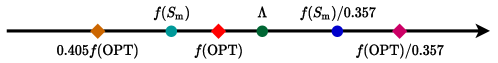
Figure 1. Relationship among $f(S_{\mathrm{m}})$, $\Lambda$, and $f(\operatorname{OPT})$.

5. Experiments

We carry out experiments on two applications to demonstrate the effectiveness of our upper bound. All the experiments are conducted on a Windows machine with an Intel Core 2.6GHz i7-7700 CPU and 32GB RAM.

Viral marketing in social networks. Viral marketing in social networks [17, 36, 40, 37, 39, 13, 14, 15, 42, 38, 41] is one of the most important topics in data mining in recent years. In this application, we consider influence maximization [17] on a social network $G=(V,E)$ with a set $V$ of vertices (representing users) and a set $E$ of edges (representing connections among users). The goal is to seed some users with incentives (e.g., discount, free samples, or monetary payment) to boost the revenue by leveraging the word-of-mouth effects on other users. We adopt the widely-used influence diffusion model called the independent cascade model [17]. Each edge $(u,v)$ is associated with a propagation probability $p_{u,v}$. Initially, the seed vertices $S$ are active, while all the other vertices are inactive. When a vertex $u$ first becomes active, it has a single chance to activate each inactive neighbor $v$ with success probability $p_{u,v}$. This process repeats until no more activation is possible. The influence spread $f(S)$ of the seed set ${S}$ is the expected number of active vertices produced by the above process. Kempe et al. [17] show that $f(S)$ is nondecreasing monotone submodular. We consider budgeted influence maximization that aims to find a vertex set $S$ maximizing $f(S)$ with the total cost $c(S)$ capped by a budget $b$, where each vertex $v$ is associated with a distinct cost $c(v)$ and $c(S)=\sum_{v\in S}c(v)$.

Note that the influence diffusion is a random process. We use the advanced sampling technique in [32] to estimate the influence spread in which $200$ random Monte-Carlo subgraphs are generated. We experiment with four real datasets from [25, 27] with millions of vertices, namely, Pokec ($1.6$M vertices and $30.6$M edges), Orkut ($3.1$M vertices and $117.2$M edges), LiveJournal ($4.8$M vertices and $69.0$M edges), and Twitter ($41.7$M vertices and $1.5$G edges). As in [17], we set $p_{u,v}$ of each edge $(u,v)$ to the reciprocal of $v$’s in-degree, and set $c(v)$ proportional to $v$’s out-degree to emulate that popular users require more incentives to participate.

Due to massive data sizes, we cannot compute the true optima. To better visualize the tightness of different bounds on the optimum, we measure the ratios of the solution values obtained by MGreedy to the upper bounds, e.g., $f(S_{\mathrm{m}})/\Lambda$, which represent the approximation guarantees achieved by MGreedy. We note that Leskovec et al. [26] developed an upper bound of $f(S_{\mathrm{g}})+\Delta(b\mid S_{\mathrm{g}})$ in our notations on the optimum. For comparisons, we evaluate both the ratios obtained for our upper bound $\Lambda$ and the upper bound developed by Leskovec et al. [26]. Figure 2 shows the results. Note that a larger ratio represents a tighter upper bound. We observe that the ratio calculated by our upper bound is usually better than $0.9$, which is much larger than both the constant factor of $0.405$ and the ratio calculated by Leskovec et al.’s bound. This demonstrates that our upper bound $\Lambda$ is quite close to the optimum for the tested cases.

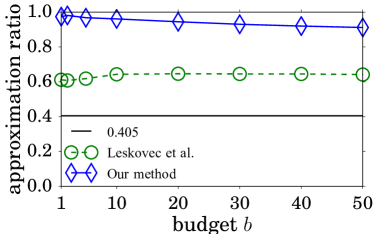
((a)) Pokec

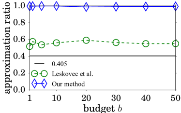
((b)) Orkut

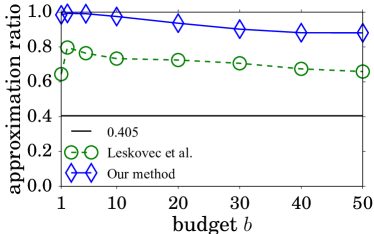
((c)) LiveJournal

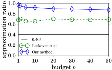
((d)) Twitter

Figure 2. Approximation ratio of modified greedy algorithm calculated by different upper bounds.

Branch-and-bound algorithm for budgeted maximum coverage. Tight bounds are valuable to advancing algorithmic efficiency. Consider the information retrieval problem where one is given a bipartite graph constructed between a set $V$ of objects (e.g., documents, images etc.) and a bag of words $W$. There is an edge $e_{v,w}$ if the object $v\in V$ contains the word $w\in W$. A natural choice of the function $f$ has the form $|\Gamma(X)|$, where $\Gamma(X)$ is the neighborhood function that maps a subset of objects $X\subseteq V$ to the set of words $\Gamma(X)\subseteq W$ presented in the objects. Meanwhile, selecting an object $v\in X$ will incur a cost $c(v)$. Intuitively, one may want to maximize the diversity (i.e., the number of words) by selecting a set of objects subject to a cost budget $b$. This problem can be seen as budgeted maximum coverage. As a proof-of-concept, we use synthetic data that define $|V|=100$ and $|W|=100$ and randomly generate an edge between $v\in V$ and $w\in W$ with probability $p=0.02$. We report the average results of $10$ instances.

We compare the branch-and-bound algorithm using our upper bound $\Lambda$ (called “Our method”) against the data-correcting algorithm (called DCA) [12] which is a branch-and-bound algorithm for maximizing a submodular function. In particular, in each branch of a search lattice $[A,B]$, the branch-and-bound algorithm needs to find an upper bound on the value of any candidate solution $S$ satisfying $A\subseteq S\subseteq B$ and $c(S)\leq b$. To achieve this goal, we first compute an upper bound $\Lambda^{\prime}$ on the optimum of $\max_{T\subseteq B\setminus A}\{f(T\mid A)\colon c(T)\leq b-c(A)\}$ as $f(T\mid A)$ is also a monotone submodular function. Then, $f(A)+\Lambda^{\prime}$ is an upper bound on the optimum of branch $[A,B]$. On the other hand, DCA uses $f(A)+\Delta(b-c(A)\mid A)$ as the upper bound, which is always (much) looser than ours. DCA considers homogeneous costs only and thus we set $c(v)=1$ for each object $v$. We manually terminate the algorithm if it cannot finish within $2$ hours. Table 1 shows the running time of DCA and our algorithm when the cost budget $b$ increases from $1$ to $10$. As can be seen, our algorithm can find the optimal solution within $2$ seconds for all the cases tested whereas DCA runs 1–4 orders of magnitude slower than our algorithm when $b\leq 5$ and even fails to find the solution within $2$ hours when $b\geq 6$.

Table 1. Running time (seconds). The field with “–” means that the method cannot finish.

Budget $b$	1	2	3	4	5	6	7	8	9	10
DCA	0.43	6.06	99.92	899.66	6807.67	–	–	–	–	–
Our method	0.04	0.06	0.09	0.11	0.17	0.32	0.51	0.77	1.21	1.90

6. Further Discussions

6.1. Upper Bound on the Approximation of MGreedy

We provide an instance of the problem for which the MGreedy algorithm achieves a ratio of $(1/2+\varepsilon)$ for any given $\varepsilon>0$. Specifically, we consider a modular set function $f$ such that $f(S)=\sum_{v\in S}f(v)$. Suppose that there are three elements $u,v,w$ with $f(u)=f(v)=1$, $f(w)=1+2\varepsilon$, $c(u)=c(v)=1$, and $c(w)=1+\varepsilon$. When $b=2$, MGreedy will select $\{w\}$ with $f(S_{\mathrm{m}})=1+2\varepsilon$, since $S_{\mathrm{g}}=\{v^{\ast}\}=\{w\}$ according to the algorithm. It is easy to verify that the optimal solution is $\{u,v\}$ with $f(\operatorname{OPT})=2$. As a result, MGreedy provides $(1/2+\varepsilon)$-approximation. We also note that Khuller et al. [19] claimed that they have constructed an instance for which MGreedy can only achieve a ratio of approximately $0.44$, but unfortunately they did not provide the detailed instance. It is unclear whether the approximation factor of $0.405$ for MGreedy is completely tight, but the above analysis shows that the gap between our ratio and the actual worst-case ratio is small.

6.2. Analysis of $\bm{(1-1/\sqrt{{\mathrm{e}}})}$ Approximation Guarantee

Khuller et al. [19] claimed that the modified greedy algorithm, referred to as MGreedy, achieves an approximation guarantee of $(1-1/\sqrt{{\mathrm{e}}})$, but unfortunately their proof was flawed as pointed out by Zhang et al. [47]. We provide here a brief explanation of the problem in the proof of [19, Theorem 3]. When showing that $f(S_{\mathrm{g}})\geq(1-1/\sqrt{{\mathrm{e}}})\cdot f(\operatorname{OPT})$ when $c(S_{\mathrm{g}})\geq b/2$, where $S_{\mathrm{g}}$ is the set obtained by the greedy heuristic and $\operatorname{OPT}$ is the optimal solution, the proof relies on $c(S_{\ell})\geq b/2$, where $S_{\ell}\subseteq S_{\mathrm{g}}$ is an intermediate set constructed by the greedy heuristic when the first element from $\operatorname{OPT}$ is selected for consideration but not added to $S_{\mathrm{g}}$ due to budget violation. However, there is a gap here, since $c(S_{\mathrm{g}})\geq b/2$ does not imply $c(S_{\ell})\geq b/2$. Interested readers are referred to the detailed analysis by Zhang et al. [47].

In this section, we provide a correct proof for the factor of $(1-1/\sqrt{{\mathrm{e}}})$. We again utilize our general approach for analyzing approximation guarantees of algorithms by solving an optimizing problem that characterizes the relations between the solution value and the optimum. The key difference for deriving the two factors (i.e., $0.405$ in Section 3 and $(1-1/\sqrt{{\mathrm{e}}})$ in this section) lies in the relations between $f(S_{\mathrm{m}})$ and $f(\operatorname{OPT})$ used in the analysis. In particular, in Section 3, we make use of two relatively complicated relations given by Corollary 3.4 and Corollary 3.6, whereas in this section, we will replace them with a new and simple relation given by the following Corollary 6.3 which will remarkably simplify the analysis.

Theorem 6.1.

The MGreedy algorithm achieves an approximation factor of $(1-1/\sqrt{{\mathrm{e}}})$.

To prove Theorem 6.1, we start with the following useful lemma.

Lemma 6.2.

Given any element set $T$, the greedy heuristic returns $S_{\mathrm{g}}$ subject to a budget constraint $b$ satisfying

$$f(S_{\mathrm{g}})\geq\Big{(}1-\frac{c(T)}{b}\Big{)}\cdot f(T).$$

Proof.

The lemma is trivial when $T\subseteq S_{\mathrm{g}}$. Suppose $T\setminus S_{\mathrm{g}}\neq\emptyset$. Let $S_{\ell}=\{u_{1},u_{2},\dotsc,u_{\ell}\}$ be the element set constructed by the greedy heuristic when the first element from $T$ is considered but not added to $S_{\ell}$ due to budget violation. Due to submodularity and the greedy rule, we have

$$\frac{f(u_{1}\mid S_{0})}{c(u_{1})}\geq\frac{f(u_{2}\mid S_{1})}{c(u_{2})}\geq\dotsb\geq\frac{f(u_{\ell}\mid S_{\ell-1})}{c(u_{\ell})}\geq\max_{v\in T^{\prime}}\frac{f(v\mid S_{\ell})}{c(v)}\geq\frac{f(T^{\prime}\mid S_{\ell})}{c(T^{\prime})},$$

where $T^{\prime}=T\setminus S_{\ell}$. Observe that

$$f(T)\leq f(S_{\ell})+f(T^{\prime}\mid S_{\ell}).$$

Meanwhile,

$$f(S_{\ell})=\sum_{i=1}^{\ell}f(u_{i}\mid S_{i-1})\geq\sum_{i=1}^{\ell}\Big{(}c(u_{i})\cdot\frac{f(T^{\prime}\mid S_{\ell})}{c(T^{\prime})}\Big{)}=c(S_{\ell})\cdot\frac{f(T^{\prime}\mid S_{\ell})}{c(T^{\prime})}.$$

Note that by the algorithm definition,

$$c(S_{\ell})+c(T^{\prime})>b.$$

Therefore,

$$f(T)<\Big{(}1+\frac{c(T^{\prime})}{b-c(T^{\prime})}\Big{)}\cdot f(S_{\ell})=\frac{b}{b-c(T^{\prime})}\cdot f(S_{\ell})\leq\frac{b}{b-c(T)}\cdot f(S_{\ell}).$$

Rearranging it concludes the proof. ∎

Based on Lemma 6.2, a relation between the greedy solution $S_{\mathrm{g}}$ and the optimal solution $\operatorname{OPT}$ can be derived as follows.

Corollary 6.3.

Let $\operatorname{OPT}^{\prime}:=\operatorname{OPT}\setminus(Q\cup\{o\})$. Then,

(26) $$f(S_{\mathrm{g}})\geq f(Q)+\Big{(}1-\frac{c(Q)}{b-c(Q)}\Big{)}\cdot f(\operatorname{OPT}^{\prime}\mid Q).$$

Proof.

According to Lemma 3.3, we know that $f(S\mid Q)$ is a monotone nondecreasing submodular set function with respect to $S$. Then, by Lemma 6.2, we have

$$f(S_{\mathrm{g}})=f(Q)+f((S_{\mathrm{g}}\setminus Q)\mid Q)\geq f(Q)+\Big{(}1-\frac{c(\operatorname{OPT}^{\prime})}{b-c(Q)}\Big{)}\cdot f(\operatorname{OPT}^{\prime}\mid Q).$$

Furthermore, by the algorithm definition, we know that

$$c(Q)+c(o)>b,$$

and $$c(o)+c(\operatorname{OPT}^{\prime})\leq c(\operatorname{OPT})\leq b.$$

Thus,

$$c(\operatorname{OPT}^{\prime})<c(Q).$$

Putting it together completes the proof. ∎

Now, we can derive a lower bound on the worst-case approximation of MGreedy by solving the following optimization problem.

Lemma 6.4.

It holds that $f(S_{\mathrm{m}})\geq\bar{\alpha}^{\ast}\cdot f(\operatorname{OPT})$, where $\bar{\alpha}^{\ast}$ is the minimum of the following optimization problem with respect to $\alpha,x_{1},x_{2},x_{3}$.

(27) $$\min\quad \alpha$$

(28) s.t. $$\alpha\geq x_{1},$$

(29) $$\alpha\geq 1-x_{1}-x_{2},$$

(30) $$\alpha\geq x_{1}+\Big{(}1-\frac{x_{3}}{1-x_{3}}\Big{)}\cdot x_{2},$$

(31) $$x_{1}\geq 1-{\mathrm{e}}^{-x_{3}},$$

(32) $$\alpha,x_{1},x_{2},x_{3}\in[0,1].$$

Analogous to the proof of Lemma 3.7, we consider $\alpha=\frac{f(S_{\mathrm{m}})}{f(\operatorname{OPT})}$, $x_{1}=\frac{f(Q)}{f(\operatorname{OPT})}$, $x_{2}=\frac{f(\operatorname{OPT}^{\prime}\mid Q)}{f(\operatorname{OPT})}$, $x_{3}=\frac{c(Q)}{b}$ here with some simpler relations between the solution value and the optimum, e.g., (29) and (30) are used instead of (13) and (15).

Lemma 6.5.

$\bar{\alpha}^{\ast}\geq 1-1/\sqrt{{\mathrm{e}}}$.

Proof of Theorem 6.1.

Combining Lemmas 6.4 and 6.5 immediately gives Theorem 6.1. ∎

6.3. Data-Dependent Upper Bound for Cardinality Constraint

In this section, we show that when the knapsack constraint degenerates to a cardinality constraint, i.e.,

$$\max_{S\subseteq V}f(S)\text{ s.t.\@ }\lvert S\rvert\leq k,$$

our upper bound $\Lambda$ is guaranteed to be smaller than $\frac{f(S_{\mathrm{g}})}{1-1/{\mathrm{e}}}$, which matches the tight approximation factor of $(1-1/{\mathrm{e}})$ [30]. Our analysis extends the result of $(1-1/{\mathrm{e}})$-approximation using an alternative proof in a concise way.

Theorem 6.6.

For monotone submodular maximization with a cardinality constraint, we have

(33) $$f(\operatorname{OPT})\leq\Lambda\leq\frac{f(S_{\mathrm{g}})}{1-1/{\mathrm{e}}}\leq\frac{f(\operatorname{OPT})}{1-1/{\mathrm{e}}}.$$

Proof.

By monotonicity, submodularity and the greedy rule, we have

$$f(S_{i})+k\cdot f(u_{i+1}\mid S_{i})\geq f(S_{i})+\Delta(k\mid S_{i})\geq\Lambda,$$

where $u_{i}$ is the $i$-the element selected by the greedy heuristic and $S_{i}:=\{u_{1},u_{2},\dotsc,u_{i}\}$, e.g., $S_{k}=S_{\mathrm{g}}$. Rearranging it yields

$$\Lambda-f(S_{i+1})\leq\left(1-1/k\right)\cdot\big{(}\Lambda-f(S_{i})\big{)}.$$

Recursively, we have

$$\Lambda-f(S_{k})\leq\left(1-1/k\right)^{k}\cdot\big{(}\Lambda-f(S_{0})\big{)}=\left(1-1/k\right)^{k}\cdot\Lambda\leq 1/{\mathrm{e}}\cdot\Lambda.$$

Rearranging it completes the proof. ∎

In each iteration of the greedy heuristic, it takes $O(n)$ time to find $u$ and the largest $k$ marginal gains [4], where $n=|V|$ is the size of ground set. There are $k$ iterations in the greedy algorithm. Thus, the total complexity of deriving $\Lambda$ is $O(kn)$, which remains the same as that of greedy algorithm.

7. Related Work

Nemhauser et al. [31] studied monotone submodular maximization with a cardinality constraint, and proposed a greedy heuristic that achieves an approximation factor of $(1-1/{\mathrm{e}})$. For this problem, Nemhauser and Wolsey [30] showed that no polynomial algorithm can achieve an approximation factor exceeding $(1-1/{\mathrm{e}})$. Feige [11] further showed that even maximum coverage (which is a special submodular function) cannot be approximated in polynomial time within a ratio of $(1-1/{\mathrm{e}}+\varepsilon)$ for any given $\varepsilon>0$, unless $\mathrm{P}\!=\!\mathrm{NP}$. Leveraging the notion of curvature, Conforti and Cornuéjols [7] obtained an improved upper bound $(1-{\mathrm{e}}^{-\kappa_{f}})/\kappa_{f}$, where $\kappa_{f}:=1-\min_{v\in V}\frac{f(v\mid V\setminus\{v\})}{f(\{v\})}\in[0,1]$ measures how much $f$ deviates from modularity. By utilizing multilinear extension [6], Sviridenko et al. [35] proposed a continuous greedy algorithm that can further improve the approximation ratio to $(1-\kappa_{f}/{\mathrm{e}}-\varepsilon)$ at the cost of increasing time complexity from $O(kn)$ to $\tilde{O}(n^{4})$, where $k$ is the maximum cardinality of elements in the optimization domain. Different from these studies, we focus on the more general problem of monotone submodular maximization with a knapsack constraint, for which the greedy heuristic does not have any bounded approximation guarantee.

Wolsey [44] proposed a modified greedy algorithm of $O(n^{2})$, referred to as MGreedy, that gives a constant approximation factor of $0.357$ for the problem of monotone submodular maximization with a knapsack constraint. Khuller et al. [19] showed that MGreedy can achieve an approximation guarantee of $(1-1/\sqrt{{\mathrm{e}}})$ for the budgeted maximum coverage problem. This factor, after being extensively mentioned in the literature, was recently pointed out by Zhang et al. [47] to be problematic due to the flawed proof. Such a long-term misunderstanding on the factor of $(1-1/\sqrt{{\mathrm{e}}})$ becomes a critical issue needed to be solved urgently. In this paper, we show that the MGreedy algorithm can achieve an improved constant approximation ratio of $0.405$ through a careful analysis, which answers the open question of whether the worst-case approximation guarantee of MGreedy is better than $(1-1/\sqrt{{\mathrm{e}}})$. In addition, we also enhance the MGreedy algorithm to derive a data-dependent upper bound on the optimum, which slightly increases the time complexity of MGreedy by a multiplicative factor of $\log n$. We theoretically show that the ratio of the solution value obtained by MGreedy to our upper bound is always larger than $0.357$, which is again tighter than the approximation factor given by Khuller et al. [19] and matches that given by Wolsey [44]. We note that Leskovec et al. [26] developed an upper bound of $f(S_{\mathrm{g}})+\Delta(b\mid S_{\mathrm{g}})$ in our notations, which is always looser than ours. Unlike our upper bound with worst-case guarantees, the relationship between $f(S_{\mathrm{g}})+\Delta(b\mid S_{\mathrm{g}})$ and $f(S_{\mathrm{m}})$ is unclear. As has been demonstrated in the experiments, our upper bound is significantly tighter than that developed by Leskovec et al. [26].

In addition to the modified greedy algorithm, Khuller et al. [19] also gave a partial enumeration greedy heuristic that can achieve $(1-1/{\mathrm{e}})$-approximation, which was later shown to be also applicable to the general submodular functions by Sviridenko [34]. Recently, Yoshida [45] proposed a continuous greedy algorithm achieving a curvature-based approximation guarantee of $(1-\kappa_{f}/{\mathrm{e}}-\varepsilon)$. However, the time complexities of the partial enumeration greedy algorithm and the continuous greedy algorithm are as high as $O(n^{5})$ and $\tilde{O}(n^{5})$, respectively. These algorithms [34, 45] are hard to apply in practice. Some recent work [3, 10] proposed algorithms with $(1-1/{\mathrm{e}}-\varepsilon)$-approximation. These algorithms are again impractical due to the high dependency on $\varepsilon$, i.e., $(\nicefrac{{\log n}}{{\varepsilon}})^{O(\nicefrac{{1}}{{\varepsilon^{8}}})}n^{2}$ [3] and $(\nicefrac{{1}}{{\varepsilon}})^{O(\nicefrac{{1}}{{\varepsilon^{4}}})}n\log^{2}n$ [10], which are of theoretical interests only.

Table 2 summarizes the results for monotone submodular maximization with a knapsack constraint. Through comparison, we find that there is still a gap between our newly derived approximation factor of $0.405$ and the best known factor of $(1-1/{\mathrm{e}})$. However, there does not exist practical algorithms that can achieve the optimal approximation ratio of $(1-1/{\mathrm{e}})$. In fact, devising efficient algorithms with approximation better than MGreedy, e.g., approaching $(1-1/{\mathrm{e}})$ or beating $1/2$, is a challenging problem.

Table 2. Comparison of approximations for monotone submodular maximization with a knapsack constraint.

MGreedy (Low Complexity)			Other Algorithms (High Complexity)
Method	Approximation	Time	Method	Approximation	Time
[44]	$0.357$	$O(n^{2})$	[34]	$1-1/{\mathrm{e}}$	$O(n^{5})$
[19]	$\frac{(1-1/{\mathrm{e}})}{2}\approx 0.316$	$O(n^{2})$	[45]	$1-\kappa_{f}/{\mathrm{e}}-\varepsilon$	$\tilde{O}(n^{5})$
Our	$0.405$	$O(n^{2})$	[3]	$1-1/{\mathrm{e}}-\varepsilon$	$(\nicefrac{{\log n}}{{\varepsilon}})^{O(\nicefrac{{1}}{{\varepsilon^{8}}})}n^{2}$
Our	$\frac{f(S_{\mathrm{m}})}{\Lambda}>0.357$	$O(n^{2}\log n)$	[10]	$1-1/{\mathrm{e}}-\varepsilon$	$(\nicefrac{{1}}{{\varepsilon}})^{O(\nicefrac{{1}}{{\varepsilon^{4}}})}n\log^{2}n$

8. Conclusion

In this paper, we show that MGreedy can achieve an approximation factor of $0.405$ for monotone submodular maximization with a knapsack constraint. This factor not only significantly improves the known factors of $0.357$ and $(1-1/{\mathrm{e}})/2\approx 0.316$ but also closes a critical gap on the misunderstood factor of $(1-1/\sqrt{{\mathrm{e}}})\approx 0.393$ in the literature. We also derive a data-dependent upper bound on the optimum that is guaranteed to be smaller than a multiplicative factor of $\frac{1}{0.357}$ to the solution value obtained by MGreedy. Empirical evaluations for the application of viral marketing in social networks show that our bound is quite close to the optimum. It remains an open question to study whether the approximation factor of $0.405$ for MGreedy is completely tight.

Appendix A Missing Proofs

Proof of Lemma 3.7.

To simplify the notations, define

$$c_{Q}:=\frac{c(Q)}{b},\ c_{o}:=\frac{c(o)}{b},\ c_{o^{\prime}}:=\frac{c(o^{\prime})}{b},\ c^{\prime}:=\frac{c(\operatorname{OPT}^{\prime})}{b},$$

$$f_{Q}:=\frac{f(Q)}{f(\operatorname{OPT})},\ f_{o}:=\frac{f(o\mid Q)}{f(\operatorname{OPT})},\ \hat{f}_{o}:=\frac{f(o\mid\emptyset)}{f(\operatorname{OPT})},\ \hat{f}_{o^{\prime}}:=\frac{f(o^{\prime}\mid\emptyset)}{f(\operatorname{OPT})},\ f^{\prime}:=\frac{f(\operatorname{OPT}^{\prime}\mid Q)}{f(\operatorname{OPT})},$$

and $$\alpha_{\mathrm{m}}:=\frac{f(S_{\mathrm{m}})}{f(\operatorname{OPT})}.$$

We show that $\alpha=\alpha_{\mathrm{m}}$, $x_{1}=f_{Q}$, $x_{2}=f_{o}$, $x_{3}=f^{\prime}$, $x_{4}=c_{Q}$, $x_{5}=c_{o}$, and $x_{6}=c_{o^{\prime}}$ are always feasible to the optimization problem defined in the lemma, which indicates that $f(S_{\mathrm{m}})\geq\alpha^{\ast}\cdot f(\operatorname{OPT})$.

By the algorithm definition,

(Constraint (12)) $$\alpha_{\mathrm{m}}\geq\frac{f(S_{\mathrm{g}})}{f(\operatorname{OPT})}\geq f_{Q},$$

(Constraint (14)) and $$\alpha_{\mathrm{m}}\geq\frac{f(v^{\ast})}{f(\operatorname{OPT})}\geq f_{o}.$$

By Corollary 3.4, we have

(Constraint (13)) $$\alpha_{\mathrm{m}}\geq f_{Q}+(1-{\mathrm{e}}^{(c_{Q}+c_{o^{\prime}}-1)/c_{Q}})f^{\prime}.$$

By Corollary 3.6, we have

(Constraint (15)) $$f_{Q}\geq(1-1/{\mathrm{e}})(1-2\alpha_{\mathrm{m}})+(c_{Q}+c_{o}+c_{o^{\prime}}-1)f_{o}/c_{o}.$$

By Corollary 3.2, we have

(Constraint (16)) $$f_{Q}\geq 1-{\mathrm{e}}^{-c_{Q}}.$$

Due to monotonicity, submodularity and the greedy rule, it is easy to get that

(Constraint (17)) $$f_{Q}+f_{o}+f^{\prime}\geq 1,$$

(Constraint (18)) and $$f_{Q}+\frac{f_{o}}{c_{o}}\geq 1.$$

Meanwhile, due to budget violation

(Constraint (19)) $$c_{S}+c_{u}>1.$$

Finally, by definition,

(Constraint (20)) $$\alpha_{\mathrm{m}},f_{Q},f_{o},f^{\prime},c_{Q},c_{o},c_{o^{\prime}}\in[0,1].$$

As can be seen, all constraints are satisfied, and hence the proof is done. ∎

Proof of Lemma 3.8.

We first consider the case $x_{4}+x_{6}-1\geq 0$. We obtain from (15) and (16) that

(34) $$x_{1}\geq(1-1/{\mathrm{e}})(1-2\alpha)+x_{2},$$

(35) and $$-\ln(1-x_{1})\geq x_{4}.$$

Then, $x_{5}\times\eqref{cons:sub2}+\eqref{cons:fs-lower-1-simple}+(1-x_{1})\times(\eqref{cons:budget}+\eqref{cons:fs-lower-2-simple})$ gives

$$x_{1}-(1-x_{1})\ln(1-x_{1})\geq 1-x_{1}+(1-1/{\mathrm{e}})(1-2\alpha).$$

Rearranging yields

(36) $$(1-x_{1})(\ln(1-x_{1})+2)-1/{\mathrm{e}}-2(1-1/{\mathrm{e}})\alpha\leq 0.$$

When $\alpha\geq 1-{\mathrm{e}}^{-3}$, we directly have $\alpha\geq\alpha^{\bot}$. When $\alpha\leq 1-{\mathrm{e}}^{-3}$, we know that $x_{1}\leq 1-{\mathrm{e}}^{-3}$ by (12). Then, $(1-x_{1})(\ln(1-x_{1})+2)$ decreases along with $x_{1}$, which indicates that

$$(1-\alpha)(\ln(1-\alpha)+2)-1/{\mathrm{e}}-2(1-1/{\mathrm{e}})\alpha\leq 0.$$

Note that the left hand side is equal to $(1-\alpha)\ln(1-\alpha)+(2-1/{\mathrm{e}})(1-2\alpha)$, which strictly decreases along with $\alpha$ when $\alpha\leq 1-{\mathrm{e}}^{-3}$. This implies that $\alpha\geq\alpha^{\bot}$.

Next, we consider the case $x_{4}+x_{6}-1\leq 0$. We prove $\alpha\geq\alpha^{\bot}$ by contradiction. Assume on the contrary that $\alpha<\alpha^{\bot}$. Then, $x_{1}<\alpha^{\bot}$ and $x_{2}<\alpha^{\bot}$. We can get from (13) and (17) that

$$x_{4}+x_{6}-1\geq\ln\Big{(}1-\frac{\alpha-x_{1}}{x_{3}}\Big{)}\cdot x_{4}\geq\ln\Big{(}\frac{1-\alpha^{\bot}-x_{2}}{1-x_{1}-x_{2}}\Big{)}\cdot x_{4}.$$

Combining it with (15) and (19) gives

$$x_{1} \geq(1-{1}/{{\mathrm{e}}})(1-2\alpha)+x_{2}\Big{(}1+\frac{x_{4}+x_{6}-1}{1-x_{4}}\Big{)}$$

(37) $$>(1-{1}/{{\mathrm{e}}})(1-2\alpha^{\bot})+x_{2}\Big{(}1+\ln\Big{(}\frac{1-\alpha^{\bot}-x_{2}}{1-x_{1}-x_{2}}\Big{)}\cdot\frac{x_{4}}{1-x_{4}}\Big{)}.$$

Note that as $\ln(\tfrac{1-\alpha^{\bot}-x_{2}}{1-x_{1}-x_{2}})\leq 0$, the left hand side of the above inequality decreases along with $x_{4}$ when $x_{4}\in[0,1)$. By (12) and (35), we have

$$x_{4}\leq-\ln(1-\alpha^{\bot}).$$

Combining with (37) gives

(38) $$x_{1}>(1-1/{\mathrm{e}})(1-2\alpha^{\bot})+x_{2}\Big{(}1+\ln\Big{(}\frac{1-\alpha^{\bot}-x_{2}}{1-x_{1}-x_{2}}\Big{)}\cdot\frac{-\ln(1-\alpha^{\bot})}{1+\ln(1-\alpha^{\bot})}\Big{)}.$$

Meanwhile, $x_{5}\times\eqref{cons:sub2}+(1-x_{1})\times(\eqref{cons:budget}+\eqref{cons:fs-lower-2-simple})$ gives

(39) $$x_{2}\geq(1-x_{1})(1+\ln(1-x_{1})),$$

where the right hand side decreases along with $x_{1}$ when $x_{1}\in[0,\alpha^{\bot})$ as required by (12). Then,

$$x_{2}\geq(1-\alpha^{\bot})(1+\ln(1-\alpha^{\bot})).$$

Define

$$x^{\bot}_{2}:=(1-\alpha^{\bot})(1+\ln(1-\alpha^{\bot})).$$

Furthermore, for the right hand side of (38), define

$$g(x_{2}):=x_{2}\Big{(}1+\ln\Big{(}\frac{1-\alpha^{\bot}-x_{2}}{1-x_{1}-x_{2}}\Big{)}\cdot\frac{-\ln(1-\alpha^{\bot})}{1+\ln(1-\alpha^{\bot})}\Big{)}$$

subject to $x_{2}\in[x^{\bot}_{2},\alpha^{\bot}]$. Taking the derivative of $g(x_{2})$ with respective to $x_{2}$ gives

$$g^{\prime}(x_{2})=1+\Big{(}\ln\Big{(}\frac{1-\alpha^{\bot}-x_{2}}{1-x_{1}-x_{2}}\Big{)}+\frac{x_{2}(x_{1}-\alpha^{\bot})}{(1-x_{1}-x_{2})(1-\alpha^{\bot}-x_{2})}\Big{)}\cdot\frac{-\ln(1-\alpha^{\bot})}{1+\ln(1-\alpha^{\bot})}.$$

Observe that $g^{\prime}(x_{2})$ decreases along with $x_{2}$. Thus, $g(x_{2})\geq\min\{g(x^{\bot}_{2}),g(\alpha^{\bot})\}$. Define

$$\tilde{g}(x_{1}):=g(\alpha^{\bot})-g(x^{\bot}_{2}).$$

Taking the derivative of $\tilde{g}(x_{1})$ with respect to $x_{1}$ gives

$$\tilde{g}^{\prime}(x_{1}) =\Big{(}\frac{\alpha^{\bot}}{1-x_{1}-\alpha^{\bot}}-\frac{x^{\bot}_{2}}{1-x_{1}-x^{\bot}_{2}}\Big{)}\cdot\frac{-\ln(1-\alpha^{\bot})}{1+\ln(1-\alpha^{\bot})}$$

$$=\frac{(\alpha^{\bot}-x^{\bot}_{2})(1-x_{1})}{(1-x_{1}-\alpha^{\bot})(1-x_{1}-x^{\bot}_{2})}\cdot\frac{-\ln(1-\alpha^{\bot})}{1+\ln(1-\alpha^{\bot})}$$

$$\geq 0.$$

Meanwhile, by (39), we can get that

$$\alpha^{\bot}>(1-x_{1})(1+\ln(1-x_{1})),$$

which indicates that $x_{1}>0.32$. Hence, $\tilde{g}(x_{1})\geq\tilde{g}(0.32)$. One can verify that

$$\tilde{g}(0.32)=\alpha^{\bot}\Big{(}1+\ln\Big{(}\frac{1-2\alpha^{\bot}}{0.68-\alpha^{\bot}}\Big{)}\cdot\frac{-\ln(1-\alpha^{\bot})}{1+\ln(1-\alpha^{\bot})}\Big{)}-x^{\bot}_{2}\Big{(}1+\ln\Big{(}\frac{1-\alpha^{\bot}-x^{\bot}_{2}}{0.68-x^{\bot}_{2}}\Big{)}\cdot\frac{-\ln(1-\alpha^{\bot})}{1+\ln(1-\alpha^{\bot})}\Big{)}>0.$$

This implies that $g(x_{2})\geq g(x^{\bot}_{2})$. Therefore, (38) can be further relaxed to

(40) $$x_{1}>(1-1/{\mathrm{e}})(1-2\alpha^{\bot})+x^{\bot}_{2}\Big{(}1+\ln\Big{(}\frac{1-\alpha^{\bot}-x^{\bot}_{2}}{1-x_{1}-x^{\bot}_{2}}\Big{)}\cdot\frac{-\ln(1-\alpha^{\bot})}{1+\ln(1-\alpha^{\bot})}\Big{)}.$$

Furthermore, define

$$\hat{g}(x_{1}):=x^{\bot}_{2}\Big{(}1+\ln\Big{(}\frac{1-\alpha^{\bot}-x^{\bot}_{2}}{1-x_{1}-x^{\bot}_{2}}\Big{)}\cdot\frac{-\ln(1-\alpha^{\bot})}{1+\ln(1-\alpha^{\bot})}\Big{)}-x_{1}$$

subject to $x_{1}\in[0,\alpha^{\bot})$. Taking the derivative of $\hat{g}(x_{1})$ with respect to $x_{1}$ gives

$$\hat{g}^{\prime}(x_{1})=\frac{x^{\bot}_{2}}{1-x_{1}-x^{\bot}_{2}}\cdot\frac{-\ln(1-\alpha^{\bot})}{1+\ln(1-\alpha^{\bot})}-1\leq\frac{x^{\bot}_{2}}{1-\alpha^{\bot}-x^{\bot}_{2}}\cdot\frac{-\ln(1-\alpha^{\bot})}{1+\ln(1-\alpha^{\bot})}-1=0.$$

This indicates that

$$\hat{g}(x_{1})\geq\hat{g}(\alpha^{\bot})=x^{\bot}_{2}-\alpha^{\bot}.$$

Putting it together with (40) gives

$$0>(1-1/{\mathrm{e}})(1-2\alpha^{\bot})+x^{\bot}_{2}-\alpha^{\bot}=(1-\alpha^{\bot})\ln(1-\alpha^{\bot})+(2-1/{\mathrm{e}})(1-2\alpha^{\bot})=0.$$

This shows a contradiction and completes the proof. ∎

Proof of Lemma 6.4.

Again, to simplify the notations, define

$$c_{Q}:=\frac{c(Q)}{b},\ c_{o}:=\frac{c(o)}{b},\ c^{\prime}:=\frac{c(\operatorname{OPT}^{\prime})}{b},$$

$$f_{Q}:=\frac{f(Q)}{f(\operatorname{OPT})},\ f_{o}:=\frac{f(o\mid Q)}{f(\operatorname{OPT})},\ f^{\prime}:=\frac{f(\operatorname{OPT}^{\prime}\mid Q)}{f(\operatorname{OPT})},\ \text{and}\ \alpha_{\mathrm{m}}:=\frac{f(S_{\mathrm{m}})}{f(\operatorname{OPT})}.$$

In what follows, we show that $\alpha=\alpha_{\mathrm{m}}$, $x_{1}=f_{Q}$, $x_{2}=f^{\prime}$, and $x_{3}=c_{Q}$ are always feasible to the optimization problem defined in the lemma, which indicates that $f(S_{\mathrm{m}})\geq\bar{\alpha}^{\ast}\cdot f(\operatorname{OPT})$.

By the algorithm definition,

(Constraint (28)) $$\alpha_{\mathrm{m}}\geq f_{Q}.$$

Due to monotonicity, submodularity and the greedy rule, it is easy to get that

$$f_{Q}+f_{o}+f^{\prime}\geq 1.$$

Together with $\alpha_{\mathrm{m}}\geq f_{o}$, we have

(Constraint (29)) $$\alpha_{\mathrm{m}}\geq 1-f_{Q}-f^{\prime}.$$

By Corollary 6.3, we have

(Constraint (30)) $$\alpha_{\mathrm{m}}\geq f_{Q}+\Big{(}1-\frac{c_{Q}}{1-c_{Q}}\Big{)}\cdot f^{\prime}.$$

By Corollary 3.2, we have

(Constraint (31)) $$f_{Q}\geq 1-{\mathrm{e}}^{-c_{Q}}.$$

Finally, by definition,

(Constraint (32)) $$\alpha_{\mathrm{m}},f_{Q},f^{\prime},c_{Q}\in[0,1].$$

As can be seen, all constraints are satisfied, and hence the lemma is proven. ∎

Proof of Lemma 6.5.

If $x_{3}>0.5$, constraints (28) and (31) directly show that $\alpha\geq 1-1/\sqrt{{\mathrm{e}}}$. Next, we consider the case $0\leq x_{3}\leq 0.5$. Then, $(1-2x_{3})\times\eqref{cons:lower2}+(1-x_{3})\times\eqref{cons:lower3}+x_{3}\times\eqref{cons:fs}$ gives

$$(2-3x_{3})\alpha\geq 1-x_{3}-x_{3}{\mathrm{e}}^{-x_{3}}.$$

Define

$$g(x):=\frac{1-x-xe^{-x}}{2-3x}$$

subject to $0\leq x\leq 0.5$. Taking the derivative of $g(x)$ with respect to $x$ gives

$$g^{\prime}(x)=\frac{1-(3x^{2}-2x+2){\mathrm{e}}^{-x}}{(2-3x)^{2}}.$$

Furthermore, the derivative of $(2-3x)^{2}g^{\prime}(x)$ with respect to $x$ is $(3x^{2}-8x+4){\mathrm{e}}^{-x}$, which is non-negative when $0\leq x\leq 0.5$. Thus, $(2-3x)^{2}g^{\prime}(x)$ achieves its maximum at $x=0.5$, i.e., the maximum is $1-1.75{\mathrm{e}}^{-0.5}<0$. This implies that $g(x)$ achieves its minimum at $x=0.5$, i.e., the minimum is $1-1/\sqrt{{\mathrm{e}}}$. Therefore, when $0\leq x_{3}\leq 0.5$, it also holds that

$$\alpha\geq 1-1/\sqrt{{\mathrm{e}}},$$

which concludes the lemma. ∎

References

- [1]
- Ageev and Sviridenko [1999] Alexander A. Ageev and Maxim I. Sviridenko. 1999. An 0.828-Approximation Algorithm For the Uncapacitated Facility Location Problem. Discrete Applied Mathematics 93, 4 (1999), 149–156.
- Badanidiyuru and Vondrák [2014] Ashwinkumar Badanidiyuru and Jan Vondrák. 2014. Fast Algorithms for Maximizing Submodular Functions. In Proc. SODA. 1497–1514.
- Blum et al. [1973] Manuel Blum, Robert W. Floyd, Vaughan Pratt, Ronald L. Rivest, and Robert E. Tarjan. 1973. Time Bounds for Selection. J. Comput. System Sci. 7, 4 (1973), 448–461.
- Boykov and Jolly [2001] Yuri Y Boykov and Marie-Pierre Jolly. 2001. Interactive Graph Cuts for Optimal Boundary & Region Segmentation of Objects in N-D Images. In Proc. IEEE ICCV, Vol. 1. 105–112.
- Calinescu et al. [2011] Gruia Calinescu, Chandra Chekuri, Martin Pál, and Jan Vondrák. 2011. Maximizing a Monotone Submodular Function Subject to a Matroid Constraint. SIAM J. Comput. 40, 6 (2011), 1740–1766.
- Conforti and Cornuéjols [1984] Michele Conforti and Gérard Cornuéjols. 1984. Submodular Set Functions, Matroids and the Greedy Algorithm: Tight Worst-case Bounds and Some Generalizations of the Rado-Edmonds Theorem. Discrete Applied Mathematics 7, 3 (1984), 251–274.
- Cornuejols et al. [1977] Gerard Cornuejols, Marshall L Fisher, and George L Nemhauser. 1977. Location of Bank Accounts to Optimize Float: An Analytic Study of Exact and Approximate Algorithms. Management Science 23 (1977), 789–810.
- Delong et al. [2012] Andrew Delong, Olga Veksler, Anton Osokin, and Yuri Boykov. 2012. Minimizing Sparse High-Order Energies by Submodular Vertex-Cover. In Proc. NeurIPS. 962–970.
- Ene and Nguyen [2019] Alina Ene and Huy L. Nguyen. 2019. A Nearly-linear Time Algorithm for Submodular Maximization with a Knapsack Constraint. In Proc. ICALP. 53:1–53:12.
- Feige [1998] Uriel Feige. 1998. A Threshold of for Approximating Set Cover. J. ACM 45, 4 (1998), 634–652.
- Goldengorin et al. [1999] Boris Goldengorin, Gerard Sierksma, Gert A. Tijssen, and Michael Tso. 1999. The Data-Correcting Algorithm for the Minimization of Supermodular Functions. Management Science 45, 11 (1999), 1539–1551.
- Han et al. [2018] Kai Han, Keke Huang, Xiaokui Xiao, Jing Tang, Aixin Sun, and Xueyan Tang. 2018. Efficient Algorithms for Adaptive Influence Maximization. Proc. VLDB Endowment 11, 9 (2018), 1029–1040.
- Huang et al. [2020a] Keke Huang, Jing Tang, Kai Han, Xiaokui Xiao, Wei Chen, Aixin Sun, Xueyan Tang, and Andrew Lim. 2020a. Efficient Approximation Algorithms for Adaptive Influence Maximization. The VLDB Journal 29, 6 (2020), 1385–1406.
- Huang et al. [2020b] Keke Huang, Jing Tang, Xiaokui Xiao, Aixin Sun, and Andrew Lim. 2020b. Efficient Approximation Algorithms for Adaptive Target Profit Maximization. In Proc. IEEE ICDE. 649–660.
- Jegelka and Bilmes [2011] Stefanie Jegelka and Jeff Bilmes. 2011. Submodularity Beyond Submodular Energies: Coupling Edges in Graph Cuts. In Proc. IEEE CVPR. 1897–1904.
- Kempe et al. [2003] David Kempe, Jon Kleinberg, and Éva Tardos. 2003. Maximizing the Spread of Influence Through a Social Network. In Proc. ACM KDD. 137–146.
- Kempe et al. [2005] David Kempe, Jon Kleinberg, and Éva Tardos. 2005. Influential Nodes in a Diffusion Model for Social Networks. In Proc. ICALP. 1127–1138.
- Khuller et al. [1999] Samir Khuller, Anna Moss, and Joseph Naor. 1999. The Budgeted Maximum Coverage Problem. Inform. Process. Lett. 70, 1 (1999), 39–45.
- Ko et al. [1995] Chun-Wa Ko, Jon Lee, and Maurice Queyranne. 1995. An Exact Algorithm for Maximum Entropy Sampling. Operations Research 43, 4 (1995), 684–691.
- Krause and Guestrin [2005] Andreas Krause and Carlos Guestrin. 2005. Near-Optimal Nonmyopic Value of Information in Graphical Models. In Proc. UAI. 324–331.
- Krause and Guestrin [2007] Andreas Krause and Carlos Guestrin. 2007. Near-Optimal Observation Selection using Submodular Functions. In Proc. AAAI. 1650–1654.
- Krause et al. [2008a] Andreas Krause, Jure Leskovec, Carlos Guestrin, Jeanne Vanbriesen, and Christos Faloutsos. 2008a. Efficient Sensor Placement Optimization for Securing Large Water Distribution Networks. Journal of Water Resources Planning and Management 134, 6 (2008), 516–526.
- Krause et al. [2008b] Andreas Krause, Ajit Singh, and Carlos Guestrin. 2008b. Near-Optimal Sensor Placements in Gaussian Processes: Theory, Efficient Algorithms and Empirical Studies. Journal of Machine Learning Research 9, 3 (2008), 235–284.
- Kwak et al. [2010] Haewoon Kwak, Changhyun Lee, Hosung Park, and Sue Moon. 2010. What is Twitter, a Social Network or a News Media?. In Proc. WWW. 591–600.
- Leskovec et al. [2007] Jure Leskovec, Andreas Krause, Carlos Guestrin, Christos Faloutsos, Jeanne VanBriesen, and Natalie Glance. 2007. Cost-effective Outbreak Detection in Networks. In Proc. ACM KDD. 420–429.
- Leskovec and Krevl [2014] Jure Leskovec and Andrej Krevl. 2014. SNAP Datasets: Stanford Large Network Dataset Collection. http://snap.stanford.edu/data.
- Lin and Bilmes [2010] Hui Lin and Jeff Bilmes. 2010. Multi-Document Summarization via Budgeted Maximization of Submodular Functions. In Proc. NAACL-HLT. 912–920.
- Lin and Bilmes [2011] Hui Lin and Jeff Bilmes. 2011. A Class of Submodular Functions for Document Summarization. In Proc. HLT. 510–520.
- Nemhauser and Wolsey [1978] George L. Nemhauser and Laurence A. Wolsey. 1978. Best Algorithms for Approximating the Maximum of a Submodular Set Function. Mathematics of Operations Research 3, 3 (1978), 177–188.
- Nemhauser et al. [1978] George L. Nemhauser, Laurence A. Wolsey, and Marshall L. Fisher. 1978. An Analysis of Approximations for Maximizing Submodular Set Functions-I. Mathematical Programming 14, 1 (1978), 265–294.
- Ohsaka et al. [2014] Naoto Ohsaka, Takuya Akiba, Yuichi Yoshida, and Ken-ichi Kawarabayashi. 2014. Fast and Accurate Influence Maximization on Large Networks with Pruned Monte-Carlo Simulations. In Proc. AAAI. 138–144.
- Shewry and Wynn [1987] Michael C Shewry and Henry P Wynn. 1987. Maximum Entropy Sampling. Journal of Applied Statistics 14, 2 (1987), 165–170.
- Sviridenko [2004] Maxim Sviridenko. 2004. A Note on Maximizing a Submodular Set Function Subject to a Knapsack Constraint. Operations Research Letters 32, 1 (2004), 41–43.
- Sviridenko et al. [2015] Maxim Sviridenko, Jan Vondrák, and Justin Ward. 2015. Optimal Approximation for Submodular and Supermodular Optimization with Bounded Curvature. In Proc. SODA. 1134–1148.
- Tang et al. [2019] Jing Tang, Keke Huang, Xiaokui Xiao, Laks V.S. Lakshmanan, Xueyan Tang, Aixin Sun, and Andrew Lim. 2019. Efficient Approximation Algorithms for Adaptive Seed Minimization. In Proc. ACM SIGMOD. 1096–1113.
- Tang et al. [2018d] Jing Tang, Xueyan Tang, Xiaokui Xiao, and Junsong Yuan. 2018d. Online Processing Algorithms for Influence Maximization. In Proc. ACM SIGMOD. 991–1005.
- Tang et al. [2016] Jing Tang, Xueyan Tang, and Junsong Yuan. 2016. Profit Maximization for Viral Marketing in Online Social Networks. In Proc. IEEE ICNP. 1–10.
- Tang et al. [2017] Jing Tang, Xueyan Tang, and Junsong Yuan. 2017. Influence Maximization Meets Efficiency and Effectiveness: A Hop-Based Approach. In Proc. IEEE/ACM ASONAM. 64–71.
- Tang et al. [2018a] Jing Tang, Xueyan Tang, and Junsong Yuan. 2018a. An Efficient and Effective Hop-Based Approach for Inluence Maximization in Social Networks. Social Network Analysis and Mining 8, 10 (2018).
- Tang et al. [2018b] Jing Tang, Xueyan Tang, and Junsong Yuan. 2018b. Profit Maximization for Viral Marketing in Online Social Networks: Algorithms and Analysis. IEEE Transactions on Knowledge and Data Engineering 30, 6 (2018), 1095–1108.
- Tang et al. [2018c] Jing Tang, Xueyan Tang, and Junsong Yuan. 2018c. Towards Profit Maximization for Online Social Network Providers. In Proc. IEEE INFOCOM. 1178–1186.
- Wei et al. [2015] Kai Wei, Rishabh Iyer, and Jeff Bilmes. 2015. Submodularity in Data Subset Selection and Active Learning. In Proc. ICML. 1954–1963.
- Wolsey [1982] Laurence A. Wolsey. 1982. Maximising Real-Valued Submodular Functions: Primal and Dual Heuristics for Location Problems. Mathematics of Operations Research 7, 3 (1982), 410––425.
- Yoshida [2016] Yuichi Yoshida. 2016. Maximizing a Monotone Submodular Function with a Bounded Curvature under a Knapsack Constraint. arXiv preprint http://arxiv.org/abs/1607.04527.
- Yu et al. [2016] Baosheng Yu, Meng Fang, Dacheng Tao, and Jie Yin. 2016. Submodular Asymmetric Feature Selection in Cascade Object Detection. In Proc. AAAI. 1387–1393.
- Zhang et al. [2018] Ping Zhang, Zhifeng Bao, Yuchen Li, Guoliang Li, Yipeng Zhang, and Zhiyong Peng. 2018. Trajectory-driven Influential Billboard Placement. In Proc. ACM KDD. 2748–2757.