Towards Geometry Guided Neural Relighting with Flash Photography

Abstract

Previous image based relighting methods require capturing multiple images to acquire high frequency lighting effect under different lighting conditions, which needs nontrivial effort and may be unrealistic in certain practical use scenarios. While such approaches rely entirely on cleverly sampling the color images under different lighting conditions, little has been done to utilize geometric information that crucially influences the high-frequency features in the images, such as glossy highlight and cast shadow. We therefore propose a framework for image relighting from a single flash photograph with its corresponding depth map using deep learning. By incorporating the depth map, our approach is able to extrapolate realistic high-frequency effects under novel lighting via geometry guided image decomposition from the flashlight image, and predict the cast shadow map from the shadow-encoding transformed depth map. Moreover, the single-image based setup greatly simplifies the data capture process. We experimentally validate the advantage of our geometry guided approach over state-of-the-art image-based approaches in intrinsic image decomposition and image relighting, and also demonstrate our performance on real mobile phone photo examples.

1 Introduction

Relighting has been an active research area in the past decades, with various applications including post-capture image editing, artistic visual effect, augmented virtual reality, rendering novel visualization for cultural heritages or commercial products, etc. [8, 29, 33, 20, 35, 36, 17, 27]. There are two categories of relighting methods: image based relighting and reconstruction based relighting. Previous image-based relighting approaches assume only photometric inputs and require capturing a dictionary containing hundreds or thousands of images of the scene at the same view point, where each image corresponds to a basic but distinct lighting condition such as a point or directional light source. Assuming the image under more complex lighting condition is a superposition of “basis images”, relighting can be done by linearly combining images in the linear intensity domain. Thus for relighting purpose, it suffices to capture these “basis images”.

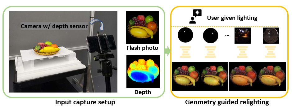
Figure 1: Illustration of our practical capture setting and the relighting application.

Capturing such large amount of images with calibrated lighting (e.g. using a light stage) requires considerable effort or cost, so many recent works try to ameliorate this issue by exploiting the local coherence structure of the light transport in the image domain [25, 30, 33].

On the other hand, the reconstruction based relighting requires the complete scene information to be given, including the geometry and material properties. The relighting can be then done by Monte-Carlo ray tracing in a physically based rendering system [26]. However, faithfully reconstructing the complete scene geometry and materials is difficult to achieve without considerable effort [11].

Therefore, both relighting methodologies are impractical in the daily photo-taking scenarios, where the environment is dynamic and taking multiple measurements correspond to the same scene is not possible. In this work we thus propose a practical approach called geometry guided image relighting. In terms of input, our approach only needs a flashlight photograph with its depth map, which can be easily obtained from a single photo shot. The outputs are the basic relit images under user-given directional light from the visible hemisphere, which can be further used for more complicated environmental relighting following the superposition rule. Our method operates entirely in the image domain, and thus needs no explicit scene reconstruction. Note that our input setting is easy to accommodate within many mobile phone cameras nowadays. This particular setting is illustrated in Figure 1. Our core contributions can be summarised as follows:

1. We propose geometry guided intrinsic image decomposition and shadow estimation under novel directional lighting, which enables competitive performance in image decomposition and relighting tasks, validated via comprehensive experiments on two large, physically accurate synthetic datasets [20, 35].

2. Our framework requires only a flashlight image and its depth map as necessary input, which is a significantly easier setup than the previous image-based relighting methods that require calibrated lighting environment, as well as the methods that rely on multiple views for reconstruction of complex scene.

The rest of this paper is organized as follows. In Section 2 we review previous work on image based relighting and surface BRDF estimation. We then explain the role of the flash photo and the depth map for the task of relighting, motivate our model design and lay out the details in Section 3.1. Important details about the datasets and training procedures are in Section 3.2. Quantitative evaluation of each module on synthetic data and experiments on real data are carried out in Section 4. The paper is concluded in Section 5 with discussion on future research.

2 Related Work

Image based relighting

Image based relighting techniques are based on the light transport equation [22]

$$\mathbf{I}=\mathbf{T}\mathbf{L}$$ (1)

where $\mathbf{I},\mathbf{T},\mathbf{L}$ denote the image vector, light transport matrix and the light vector, respectively, with their values all in the linear intensity domain. This equation essentially means the superposition principle for combining images under different lighting. Earlier works [8, 29] densely sample the light transport matrix in order to perform relighting. Such brute-force alike methods perform very well in general, and work with essentially arbitrary geometries and materials, but the sample size is usually huge. Often these approaches require dedicated hardware, calibrated lighting, significant capture time and storage.

To reduce such hard effort, recent approaches [25, 33, 10, 30, 28] aim to exploit the local coherence structure of the light transport by making use of the data-driven representations, reducing the required sampling to a few hundred images for a single scene. A very recent work [35] uses deep learning to represent such structure within large synthetic datasets, and meanwhile it learns the optimal sparse lighting directions, reducing the input to as few as five images, which is referred to as the optimal sparse sampling (OSS) approach. However, for the above purely image-based methods, calibrated lighting condition is still essential and thus can be still unrealistic in many practical cases. We therefore propose to capture a single flashlight photo and its depth map to alleviate the requirement of multiple calibrated lighting.

Finally, there are also recent works that utilize the expressive power of deep neural networks for directly relighting more constrained objects like human faces from a single image [31, 32, 36].

Intrinsic image decomposition

Estimating the intrinsic images that can be used to model an observed image is an active research area for decades. It is often called inverse graphics because they are inverse problems to the forward graphics models. The more complex the material and geometry a scene has, the more complicated the forward graphics model will become. For example, the simple shading model [3]

$${\bf I}={\bf R}\odot{\bf S}$$ (2)

which decomposes the image ${\bf I}$ of mainly diffusive objects into its multiplicative components of reflectance ${\bf R}$ and shading ${\bf S}$. The shading term can be further decomposed into lighting configuration and surface normal. Earlier works develop optimization models which estimate the shading (and therefore surface normal) assuming the Lambertian surface property, e.g. [16] with known lighting, or [2] with unknown lighting, or with more complex materials [15]. See also references therein for more comprehensive review on this matter. These previous works accomplish their tasks under simplifying assumptions and hand-crafted priors, thus less applicable to model general scenes. On the other end, the image modelling can be as complex as the entire physically based rendering system. Such is the approach of differentiable rendering [23], which can potentially support a range of hard inverse graphics problems.

Material estimation itself has also been the focus of many previous works. These methods involve modelling the material, usually as a microfacet BRDF model [18]. For instances, [24] reconstructs the material assuming known geometry and lighting. [14] estimates spatially varying BRDF parameters from multiple flashlight image co-located with camera for near planar scenes. [13] performs BRDF estimation from images under different lighting using dictionary learning. Recent methods tend to utilize the representation power of deep networks trained on large datasets, e.g. the very recent works [9, 19] that reconstruct spatially varying BRDF parameters for near planar scenes. [20] proposes a large synthetic dataset to learn shape, surface normal, diffuse albedo and specular roughness altogether from a single flash photograph, which is referred to as single image photometric stereo, abbreviated SIPS.

Our relighting framework includes an intrinsic image decomposition step and follows closely the setting in [20]. But our work is different in one key aspect in that we require the depth map corresponding to the flashlight image, which turns out to be very beneficial for the estimating the other intrinsic images. Note that making use of depth cue for intrinsic image decomposition tasks have been explored in [1, 6] and many others. However these work consider only the simple shading model (2) and thus fall short of material reconstruction for relighting.

Finally, one can perform full reconstruction of geometry, material and environmental lighting as in [34] using a Kinect sensor, whose capture takes considerable time. One can also acquire full surface reflectance as in [8, 21, 11] using a light stage, which is in fact closely related to the image-based relighting method. While of great quality, such highly calibrated conditions is very hard to obtain and implement in common scenarios.

3 Framework

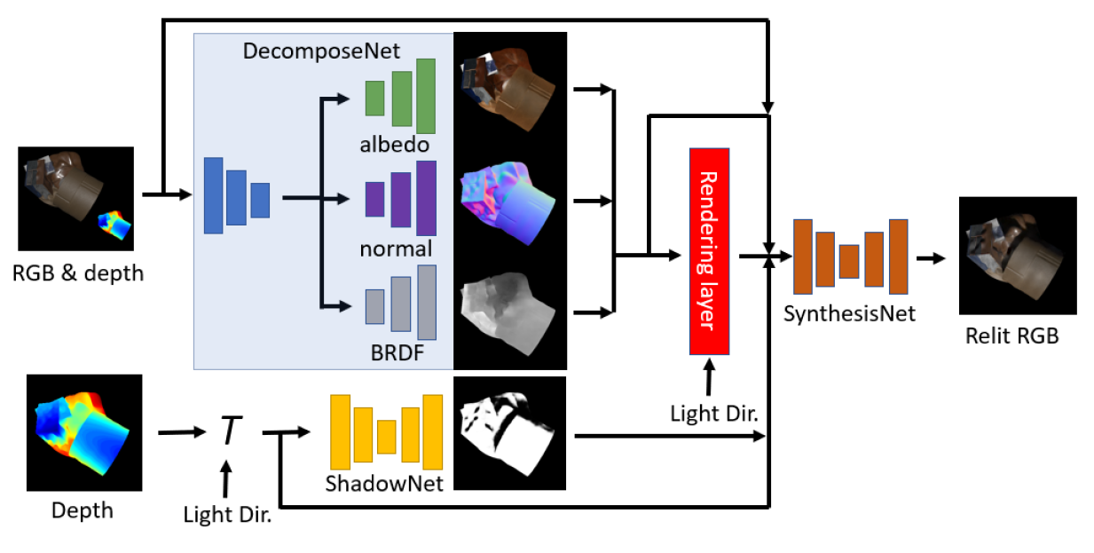
Figure 2: Model architecture overview. Our model can be conceptually divided into three parts: DecomposeNet, where geometry guided intrinsic image decomposition is performed; ShadowNet, which learns the global geometric relation between scene points after the shadow encoding transform $T$; SynthesisNet, which re-combines the different intrinsic components and synthesizes the relit image under the user given lighting direction.

As alluded in Section 1, the desired model must be capable of relighting with a single camera shot, which leads to our design decisions. In terms of the framework, we have aimed for one that operates entirely in the image space, since the reconstruction can hardly be done well enough for a complex scene, which often results in unpleasant artifacts, c.f. Fig.3. In terms of the capture setup, we have required the color image to be taken under a (or almost) co-located flashlight, for three reasons: 1) the constrained lighting helps ease the complexity of scene intrinsics estimation; 2) since the flash and the camera are (almost) co-located, the flashlight image contains (almost) no shadow, thus it eliminates the hard work to distinguish shadows from textures; 3) such flashlight images are easy to obtain with many mobile devices. We can further assume the only light source in the input image is the flashlight, since it may be obtained by taking two photos at essentially the same time, one with flash and one without, and subtracting them in the linear intensity domain.

3.1 Model design

Now given a flashlight image ${I}_{\text{flash}}$ and its (possibly noisy) depth map $D$, our task is to predict the same capture but under novel, user-given lighting. To achieve this goal we incorporate geometry from the depth map that will guide our model to reason about the global high frequency component in a relit image, namely the shadow and glossy highlight.

Since we have aimed for an image based approach, we have to compute the shadow in the image domain without resorting to reconstruction. Thus we design ShadowNet, which learns a binary cast shadow image, where zero value indicates shadow, solely from the depth map of the flash image and the given light direction ${\omega}$. Note that the cast shadow is a function of the global geometry of our opaque scene. ShadowNet will output a cast shadow map $I_{\text{shadow}}$ from the properly transformed depth map $T(\omega,D)$ such that it encodes the information of the novel lighting.

$$I_{\text{shadow}}=\mathbf{ShadowNet}(T(\omega,D))$$ (3)

Besides a shadow map, we need also to learn the other non-trivial local appearance change due to the new lighting direction. This leads to our second component, DecomposeNet, which perform principled scene analysis based on a pre-defined appearance model. Specifically, it infers the diffuse albedo map, surface normal map and spatially varying BRDF map of the captured scene. In this work we adopt the microfacet BRDF model of [18]. This BRDF model is controlled by a parameter called roughness, which is the subject of our prediction. Its value ranges in $(0,1]$, and the smaller the value, the more specular the material will appear.

$$I_{\text{albedo}},I_{\text{normal}},I_{\text{roughness}}=\mathbf{DecomposeNet}(I_{\text{flash}},D)$$ (4)

Since the previous components output the appearance under direct lighting, we need to add the global, indirect lighting effect to form the final image. The last component, SynthesisNet, reconstructs the image under novel directional lighting.

$$I_{\text{relit}}=\mathbf{SynthesisNet}(\omega,D,I_{\text{albedo}},I_{\text{normal}},$$ (5)

$$I_{\text{roughness}},I_{\text{shadow}},I_{\text{flash}})$$

The structure of our model is illustrated in Figure 2. We next explain in details the design principle and loss function of each individual component. More details can be found in the supplementary material.

Learning cast shadow

One of the most significant factors that contributes to the visual realism of a synthesized image is cast shadow. There are many ways to encode the visibility information and we choose the following method that works well in practice. We first convert the depth image $D$ to the corresponding point cloud image, namely a three-channel image with each channel stores the $x,y,z$ coordinates in the camera’s Euclidean coordinate system. Suppose the light is in direction $\omega$. We complete it into an orthonormal basis, in the form of a matrix $R$ such that the third column is $\omega$. We then transform a point $p=(x,y,z)^{T}$ by

$$T:p\mapsto R^{T}p+t$$ (6)

where $t$ is a suitable translation. In our case we simply use $t=(0,0,1)^{T}$. Note that this transform can be implemented as a convolution layer of kernel size $1\times 1$.

The transformed point coordinates, which is again a three-channel image, will be the input of an hour-glass shaped convolutional neural network with skip links (U-Net) to predict a shadow image. We use the pixel-wise binary cross-entropy loss $\mathcal{L}_{\text{shadow}}$ for supervised training. More details about its design motivation and computation of $R$ can be found in the supplementary material.

Learning image decomposition

Having described how to generate the shadow image, which is about learning the geometric relations between scene points that are possibly far apart, now we head to the more local image analysis task of intrinsic image decomposition, making use of the flashlight color image.

Since the three tasks, namely estimating diffuse albedo, surface normal and roughness, are not mutually exclusive, we use a shared encoder that branches into three different decoders, as shown in part of Figure 2.

The shared encoder then takes $I_{\text{flash}},P$ as inputs, and the feature from the last layer are fed into three individual decoders, with skip-links connected to intermediate layers of the encoder to ensure that the high-frequency details are preserved. It is worth mentioning that, although we assumed the depth image in the input, surface normal estimation will benefit from the flashlight color image. One obvious reason is that the depth map obtained may contain noise. But the benefit even holds true for synthetic data with perfect depth, since the depth map only represents the large-scale smooth geometry, while the micro-scale non-smooth geometry are represented separately using surface normal textures [5].

The roughness prediction branch is supervised by pixel-wise binary cross-entropy loss $\mathcal{L}_{\text{roughness}}$. The normal prediction branch and the diffuse albedo prediction branch use $L^{1}$ loss on both pixel value and image gradients, denoted by $\mathcal{L}_{\text{normal}}$ and $\mathcal{L}_{\text{albedo}}$.

Image synthesis under novel lighting

Once we have the diffuse albedo, surface normal and roughness maps, we can already compute in close form a $1$-bounce image $I_{\text{render}}$ of the imaged scene under light from arbitrary direction $\omega$, though without cast shadow. To add the cast shadow, enhance the quality, we pass the concatenation of $I_{\text{shadow}}$, $I_{\text{render}}$, $I_{\text{flash}}$, $I_{\text{albedo}}$, $I_{\text{normal}}$, $I_{\text{roughness}}$ and $T(\omega,D)$ to a final U-Net structure SynthesisNet to predict the final image under lighting from direction $\omega$. This network is also trained using a combination of $L^{1}$ losses on both image and image gradient, denoted by $\mathcal{L}_{\text{relight}}$.

3.2 Datasets and training procedures

It is often essential to have a large amount of high quality data sampled from diverse scenarios for a deep learning method to work well. For the image relighting task, there are usually hundreds or thousands of “basis images” that come with a single view of a scene. Consequently, to collect a large dataset containing diverse scenes is very challenging. To address this issue, Xu et al. [35] proposed a large photo-realistic synthetic dataset. The major part of Xu’s dataset contains 500 training scenes and 100 testing scenes, each generated by taking random combinations of shapes, surface normal maps, diffuse albedo textures and specular roughness maps. For each scene, a total of 1053 images are rendered with directional lighting over the visible hemisphere. We consider Xu’s dataset to be one of the ideal datasets for training the relighting model with directional lighting. To adapt Xu’s dataset to our task, we additionally render the depth map for each scene, using the geometry provided in their dataset, as well as the binary shadow image for each lighting direction.

Unfortunately, Xu’s dataset does NOT contain those ground truth surface normal maps, diffuse albedo textures and specular roughness maps. This means that we cannot directly supervise our DecomposeNet using Xu’s dataset alone. We address this problem by utilize another complimentary dataset proposed by Li et al. [20]. It contains ground truth intrinsic images but not the relighting, and a different BRDF model than [35]. To train our model with these two datasets, we adopt a stage-wise training strategy as follows.

In the first stage, we train the module ShadowNet on Xu’s data using loss $\mathcal{L}_{\text{shadow}}$, and DecomposeNet on Li’s data using loss $\mathcal{L}_{\text{albedo}}+\mathcal{L}_{\text{normal}}+\mathcal{L}_{\text{roughness}}$, both for 5 epochs. The training on two datasets can be done in parallel. In the second stage, we fix the pretrained networks ShadowNet and DecomposeNet from the first stage and train SynthesisNet on Xu’s data using $\mathcal{L}_{\text{relight}}$ for 5 epochs. For all training, the batch size is set to be $4$, and we use the Adam optimizer with default hyper-parameters with initial learning rate $5\times 10^{-4}$ and decay it by $\times 0.1$ every two epochs. Totalling at $27M$ parameters, our model is relatively more compact in sizes than the models released by [35] ($33M$) and [20] ($64M$). We will open source our implementation to promote future research in this direction.

4 Evaluation and results

4.1 Influence by the quality of depth input

Since our framework requires depth map as input, a first question would be how the quality of depth affects the results, in terms of both training and testing, since for real data it is difficult to obtain perfect depth as ground-truth. In this respect, we quantitatively evaluate our ShadowNet, DecomposeNet and SynthesisNet modules. We train two models using identical procedures, one (Clean) with clean depths and the other (Noisy) with random Gaussian noise and Gaussian blur applied. For input depth in range $[0,1]$ of size $256\times 256$, we choose $\mu=0,\sigma=6.25\times 10^{-2}$ for Gaussian noise and $\sigma=1$ for Gaussian blur. An instance for clean and noisy depths is illustrated in the bottom-left of Fig.5. During testing, Clean uses original testing data and Noisy uses the same except for the noisy depth under the same perturbation scheme. The numerical results in Mean Squared Error (MSE) are shown in Table 1 with PSNR visualization for each testing lighting direction in Fig.7. Typical testing results are shown in Fig.4 and 5.

From Table 1, we can observe that for DecomposeNet, the albedo and BRDF roughness estimation tend to be more robust to the noise in depth. In fact, the albedo task even sees an increase in performance. The increase in performance of diffuse albedo estimation is possibly due the nature of the task. The diffuse appearance of the flash image is less affected by local depth fluctuations and thus noisy geometry can be treated as an effective data augmentation. Note this is not the case for the normal estimation and roughness estimation. The ShadowNet also has a drop in performance and thus affects SynthesisNet. This is expected, since shadow map prediction should rely on accurate geometry. Note that all results from DecomposeNet compare favorably to SIPS [20], which is a considerably more complicated model. This demonstrates the effectiveness of geometry guided image decomposition.

MSE	Albedo	Normal	Roughness	Shadow	Relight
Gray Clean.	$0.72\times 10^{-2}$	$\mathbf{1.53\times 10^{-2}}$	$\mathbf{4.18\times 10^{-2}}$	$\mathbf{1.26\times 10^{-2}}$	$\mathbf{0.40\times 10^{-2}}$ [t]
Noisy.	$\mathbf{0.48\times 10^{-2}}$	$1.85\times 10^{-2}$	$4.23\times 10^{-2}$	$5.53\times 10^{-2}$	$0.54\times 10^{-2}$ [t]
[20]	${4.84\times 10^{-2}}$	${3.81\times 10^{-2}}$	${1.93\times 10^{-1}}$	$N/A$	$N/A$ [t]

Table 1: Influence by the quality of depth input. The quality of depth has a notable effect on normal and shadow estimation.

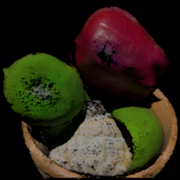
(a)

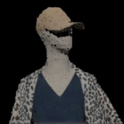
(b)

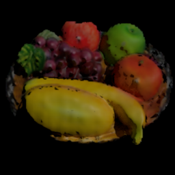
(c)

Figure 3: Reconstruction based relighting results. Note the sever artifacts due to the difficulty of generating a good mesh from a single noisy depth for complex shapes. For comparison, our results are shown in Fig.9

(a)

(b)

(c)

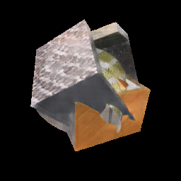
(d)

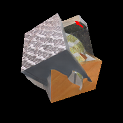
(e)

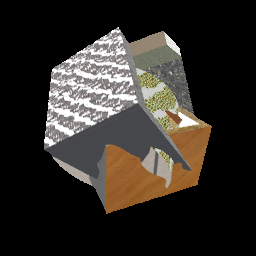
(f)

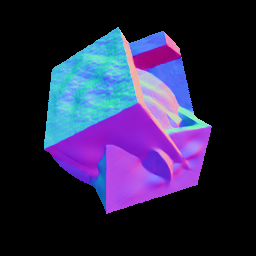
(g)

(h)

(i)

(j)

(k)

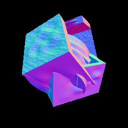
(l)

(a) Clean.

(b) Noisy

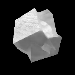
(c) Env.

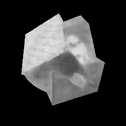
(d) [20]Init.

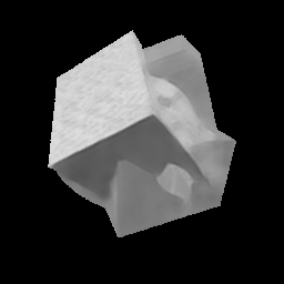
(e) [20]Refine.

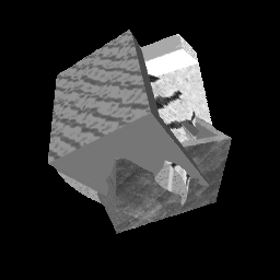
(f) Truth

Figure 4: Visual comparison for DecomposeNet under different input configurations on Li’s testing dataset [20]. Each row shows albedo, normal and roughness map respectively. The initial and final results from the three-stage model of [20] are also included for comparison. Note our albedo and normal estimation are much more accurate than [20] thanks to the geometry guidance. Note the arrows marked in (c). Please zoom-in for better details.

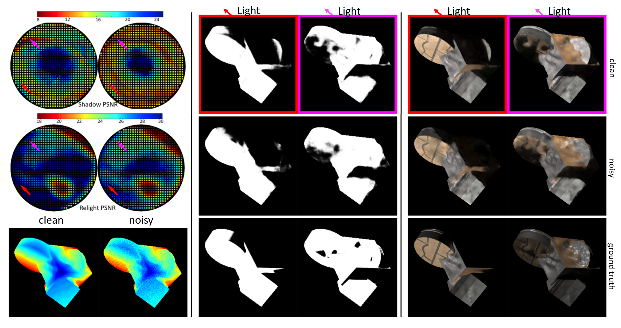
Figure 5: Visual comparison for ShadowNet and SynthesisNet trained with clean and noisy depths. On the left we show the PSNR-direction plot for the current scene, with clean and noisy depth inputs illustrated at the bottom. The shadow estimation and relighting under novel light directions (marked on the PSNR plot) are shown in the middle and right columns. The first row represents results of Clean, and second row Noisy, and the last row ground-truth.

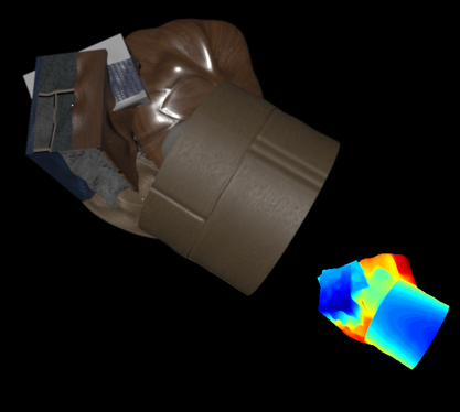
(a)

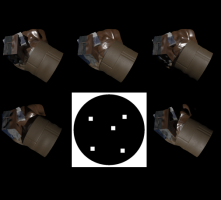
(b)

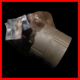
(c)

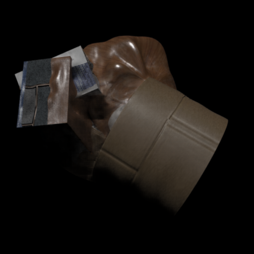
(d)

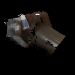
(e)

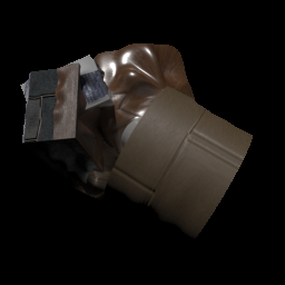
(f)

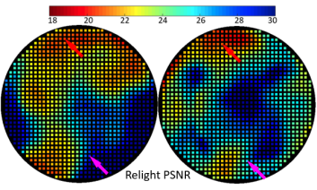
(a) Ours vs. OSS[35]

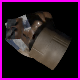
(b) Ours

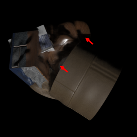
(c) OSS [35]

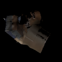
(d) SIPS [20]

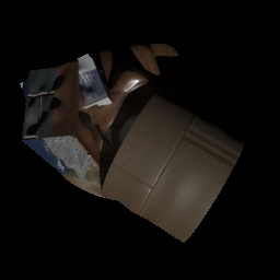
(e) Truth

Figure 6: Visual comparison of relighting performance. The input setting between ours and OSS is illustrated on the top-left, and the PSNR-direction plot on the bottom-left. Two large angle lighting directions are chosen for visualization. Please zoom-in for better details.

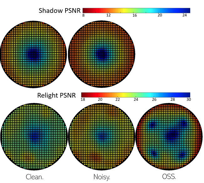
(a)

Figure 7: Average PSNRs with respect to lighting directions for both ShadowNet and SynthesisNet on Xu’s testing dataset [35]. The result from OSS in the default setting (five input images under different calibrated directional lighting) is included for comparison.

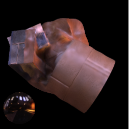
(a)

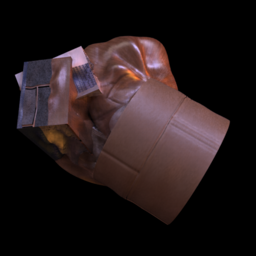
(b)

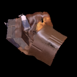
(c)

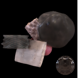
(a) Ours

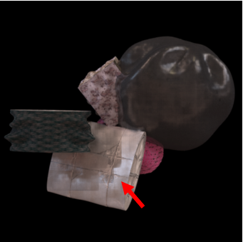
(b) OSS [35]

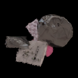
(c) SIPS [20]

Figure 8: Comparison for relighting under novel environmental light. Note the block-ish artifact from OSS in the second row (b), because it makes no use of geometric information. SIPS reconstruction does not work well when the underlying scene geometry is complex, along with other technical problems during the scene reconstruction. Please zoom-in for better details.

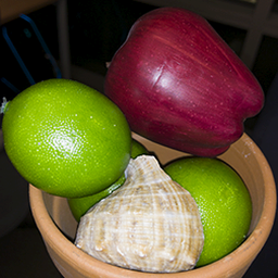
(a)

(b)

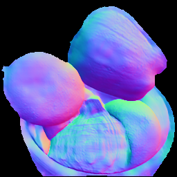
(c)

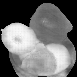
(d)

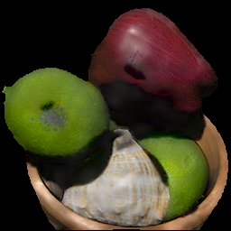
(e)

(f)

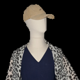
(g)

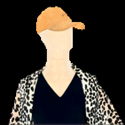
(h)

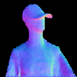
(i)

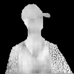
(j)

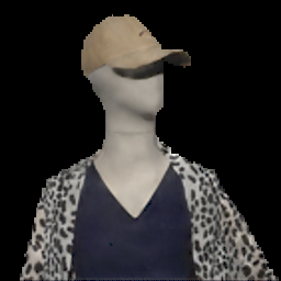
(k)

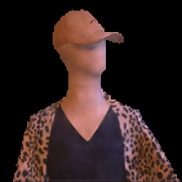
(l)

(a) Flash

(b) Albedo

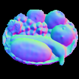
(c) Normal

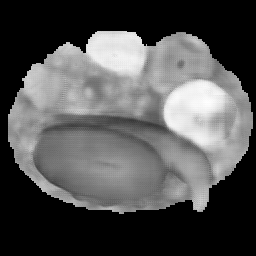
(d) Roughness

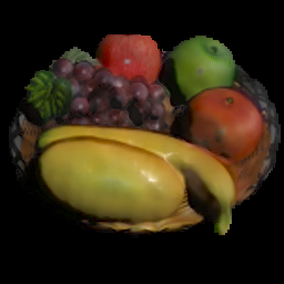
(e) Dir. light

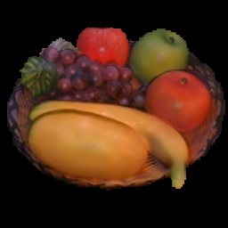
(f) Env. light

Figure 9: Visual evaluation of our model on real data under novel directional light and environmental light. The image and depth in the first row is taken from the real dataset provided in [20]. The images and depths in the last two rows are taken by our mobile phone camera with Time-of-Flight sensor.

4.2 Comparison with reconstruction based method

For this baseline approach we reconstruct the scene using MeshLab [7] from the input noisy depth map. Specifically, we choose the ball-pivoting method [4] which yields the best empirical meshing result. We texture map our inferred albedo, normal and material images, and relight the scene via physically based rendering. The results on our real data captured using a mobile phone are shown in Fig.3. As can be seen, there are severe artifacts in the cast shadows and holes in the surface, since it is difficult to produce a nice mesh from a single noisy depth map of a complex scene. In contrast, we show our results under the same lighting in Fig.9 where such artifacts are effectively avoided. This should justify our use of image-based approach.

4.3 Relighting performance evaluation

To conduct quantitative evaluation, ground truth relighting results are necessary. Since most real datasets do not contain geometry that fits our input setting, we therefore utilize photo-realistic synthetic data for this purpose, following the practice of [35]. The main state-of-the-art relighting approach to compare is optimal sparse sampling (OSS) [35], which in its default setting utilizes five input images, each under calibrated directional light source. Note that its capture setting is much more complicated than ours. We compare the input setting of OSS with ours in the top-right corner of Fig.6. We visualize results of the three approaches under the large angle lighting in Fig.6. The average PSNR over the Xu’s testing dataset of each direction is shown in Fig.7. We also compare the environmental relighting performance qualitatively with OSS and visualize it in Fig.8. More comparison can be found in the supplementary video.

Quantitatively, as shown in Fig.7, our relighting results compare favourably with OSS for small lighting angels and is satisfactory when the angle is large. We observe that OSS has more block-ish artifacts in shadow, as marked by red arrows in the second row of Fig.6(c), and the second row of Fig.8(b), since geometric information is absent from the shadow synthesis in OSS. Thanks to multiple samples, OSS is better at producing more faithful highlights. Note that our highlight computation uses the original BRDF as in Li’s dataset [20]. Since the OSS has different BRDFs with no ground truth given, our rendering layer computes the rendering that is incompatible with OSS. SynthesisNet can compensate for this defect to a certain extent, though not able to perfectly close the gap, causing blurry highlight in the final results under large angle lighting. Better performance can be expected if a unified dataset is available.

We also consider the related approach SIPS based on scene reconstruction from a single flashlight image [20], where the depth estimated from the color image and not taken into account for guiding the decomposition task. The depth estimation of this method usually degrades severely when the scene is complex and the relighting completely fails. Here we show the qualitative results in Fig.6 and Fig.8 using the same reconstruction pipeline detailed in Section 4.2. We can observe that SIPS behaves poorly in the relighting task for the complex shapes in Xu’s dataset, and the associated technical problems e.g. holes, from the scene reconstruction further degrades the visual quality. This demonstrates the advantage of our image based method without need for reconstruction.

Finally, in Fig.9 we demonstrate some results by directly applying our trained model on real images captured by mobile phone cameras. Notice the realistic cast shadows we produce between the individual objects as well as the glossy highlights under novel directional and environmental lighting. Please refer to our supplementary video for more thorough visualization results.

5 Conclusion and future work

We have proposed a framework for geometry guided neural image relighting with flash photography. The flashlight provides us a simple constrained lighting condition for material inference, and the geometry guidance from the depth map allows our model to reason about the global image appearance under a novel lighting condition. Our modular design allows the model to learn different high frequency effects like cast shadows and glossy highlights separately, while remains conceptually simple.

There are several future directions which can be explored. The first would be extending this framework to the multi-modal sensor domain, for example a Time-of-Flight(ToF) RGB-D camera module. In this case the infrared image may provide additional cues for material inference, and can potentially further alleviate the flashlight constraint. Secondly, creating a physically accurate synthetic dataset with full lighting conditions and ground-truth material and geometries, as well as large real dataset with full lighting conditions and geometry, can be extremely helpful to promote future research in this direction.

Appendix A Additional explanation on our model design

A.1 Why we need shadow estimation and intrinsic image decomposition

To motivate our model design, we need first introduce some elements of the physically based rendering model for an opaque scene. Let $L(p^{\prime}\to p)$ denote the radiance from point $p^{\prime}$ to $p$ in an opaque scene $\mathcal{A}$. Its resulting exiting radiance $L(p\to p^{\prime\prime})$ from $p$ to another $p^{\prime\prime}$ can be computed as a certain fraction of $L(p^{\prime}\to p)$ [26]:

$$L(p\to p^{\prime\prime})=f(p^{\prime}\to p\to p^{\prime\prime})G(p^{\prime}\to p)L(p^{\prime}\to p)$$ (7)

There are two distinctive factors in the above expression. The first is $f(p^{\prime}\to p\to p^{\prime\prime})$, the BRDF at $p$, which encodes the material property. Such a BRDF can be decomposed into diffusive and glossy components. The diffusive component (which is equivalent to the diffuse albedo) is simply the constant term in a BRDF. Hence the more glossy a BRDF is, the more it depends the geometric relation between the points $p^{\prime},p$ and $p^{\prime\prime}$. The second $G(p^{\prime}\to p)$ term encodes the geometric relation between $p^{\prime}$ and $p$, including global intensity fall-off related to the distance between $p^{\prime}$ and $p$; Lambert’s cosine law, which concerns the surface normals at $p$ and $p^{\prime}$; most importantly, their mutual visibility, which is a dominating term in $G$ when the scale of the scene is small.

Now in Expression (7), consider the source light ray $p^{\prime}\to p$ to be in direction $\omega$, and $p^{\prime\prime}$ is our camera. This equation corresponds to the $1$-bounce (i.e. direct illumination) image under directional lighting. The outgoing radiance $L(p\to p^{\prime\prime})$ will vary smoothly with respect to $\omega$, except when the mutual visibility term changes its value, or enters/exits the glossy component of the BRDF. In the image space, the first kind of discontinuity appears in the form of cast shadow, and the latter appears in the form of glossy highlights. These discontinuities are the main source of local incoherence in light transport. Hence for relighting, we argue that predicting them will be necessary to alleviate multiple captures under calibrated lighting. A naive model without factoring the relighting into these components exhibit very poor results on complex scenes.

If the geometry of the scene is available, it is possible to have a more reliable estimate of the BRDF $f$ and the geometric term $G$. First of all, material inference can be made under particular profile of intensity, light direction and surface local geometry, which makes the challenging problem of material estimation easier to solve than purely based on color images [20]. Also, the mutual visibility term can also be estimated by reasoning the geometric relations between the scene points. Thus our model first performs analysis on both image and geometry to obtain estimation on the BRDF and visibility terms, which result in the glossy highlight and cast shadow in an image under novel lighting.

A.2 Why encoding cast shadow as view-dependent scene coordinates

In computer graphics, the computation of the cast shadow map has been successful with well-modeled geometry. The main computation is to check whether the ray between a scene point and the light source is blocked by some other opaque scene surface. In screen space rendering, checking whether the pixel $(i,j)$ is in shadow is done by comparing the smallest depth value rendered from the light perspective, called shadow mapping (which requires a new rendering pass), with the true depth value at $(i,j)$. If the shadow mapping’s value is smaller, then the pixel should be in shadow.

However, shadow computation has been less explored with a single depth map without resorting to scene reconstruction, which is often a challenging task in application scenarios. Here we propose to directly learn the shadow image from depth map and the given light direction $\omega$. The key to our approach is a transform $T$ of the depth map defined by $\omega$. The principle is the same with that of the screen space method: the shadow created by a directional light is the same with the occlusion seen from an orthographic camera from the light direction. So we can encode this shadow information by transforming the scene points from the camera’s Euclidean coordinate system to the light’s Euclidean coordinate system. We then use a neural network to retrieve the encoded shadow image. The computation of matrix $R$ can be done as follows. Given the vector $\omega$, we find two basis vectors $e_{i},e_{j}$ out of the standard coordinate frame to from $(e_{i},e_{j},\omega)$ so that they are linearly independent. Then we apply the Gramm-Schmidt orthogonalization procedure to form the matrix $R$. In our implementation, we simply use the python provided function linalg.null_space. Although it may be the case for nearby directions different $R$’s are generated, we find it has little impact to the results and can be treated as a form of data augmentation.

Appendix B Network details

We use the Leaky-ReLU non-linearity with negative slope $-0.1$. All convolutional parameters are initialized using He’s method [12], the bias terms are initialized to be zero. Albedo and relighting prediction layers has no non-linearity and no bias term; normal prediction layer has per pixel normalization to have unit Euclidean norm; roughness and shadow prediction layers have sigmoid activation. The specific structure are detailed in the following table.

DecomposeNet: RGB encoder
Layer	K	S	Channels	I	O	Input Channels
rgb_conv0	6$\times$6	2	4/32	1	2	$I_{\rm RGB}$, $I_{\rm D}$ [t]
rgb_conv1	4$\times$4	2	32/64	2	4	rgb_conv0
rgb_conv2	4$\times$4	2	64/128	4	8	rgb_conv1
rgb_conv3	4$\times$4	2	128/256	8	16	rgb_conv2
rgb_conv4	4$\times$4	2	256/512	16	32	rgb_conv3
DecomposeNet: 3 copies of albedo, normal and roughness decoders
upconv0	4$\times$4	2	512/256	32	16	rgb_conv4
upconv1	4$\times$4	2	256/128	16	8	rgb_conv3, upconv0
upconv2	4$\times$4	2	128/128	8	4	rgb_conv2, upconv1
upconv3	4$\times$4	2	128/64	4	2	rgb_conv1, upconv2
upconv4	4$\times$4	2	64/64	2	1	rgb_conv0, upconv3
DecomposeNet: albedo, normal and roughness estimation layers
Albedo	5$\times$5	1	64/3	1	1	upconv4
Normal	5$\times$5	1	64/3	1	1	upconv4
roughness	5$\times$5	1	64/1	1	1	upconv4

ShadowNet
Layer	K	S	Channels	I	O	Input Channels
conv0	6$\times$6	2	3/32	1	2	$T(\omega,T_{\rm D})$
conv1	4$\times$4	2	32/64	2	4	conv0
conv2	4$\times$4	2	64/128	4	8	conv1
conv3	4$\times$4	2	128/256	8	16	conv2
conv4	4$\times$4	2	256/256	16	32	conv3
upconv0	4$\times$4	2	256/256	32	16	conv4
upconv1	4$\times$4	2	256/256	16	8	conv3, upconv0
upconv2	4$\times$4	2	256/128	8	4	conv2, upconv1
upconv3	4$\times$4	2	128/64	4	2	conv1, upconv2
upconv4	4$\times$4	2	64/32	2	1	conv0, upconv3
shadow	6$\times$6	2	32/1	1	1	upconv4

SynthesisNet
Layer	K	S	Channels	I	O	Input Channels
conv0	6$\times$6	2	17/64	1	2	$I_{\rm RGB},T(\omega,T_{\rm D})$, etc.
conv1	4$\times$4	2	64/128	2	4	conv0
conv2	4$\times$4	2	128/128	4	8	conv1
conv3	4$\times$4	2	128/256	8	16	conv2
conv4	4$\times$4	2	256/256	16	32	conv3
upconv0	4$\times$4	2	256/512	32	16	conv4
upconv1	4$\times$4	2	512/256	16	8	conv3, upconv0
upconv2	4$\times$4	2	256/128	8	4	conv2, upconv1
upconv3	4$\times$4	2	128/64	4	2	conv1, upconv2
upconv4	4$\times$4	2	64/32	2	1	conv0, upconv3
relight	5$\times$5	2	32/3	1	1	upconv4

Table 2: Network architecture. K means kernel size, S means stride, and Channels is the number of input and output channels. I and O are the input and output downsampling factor relative to the initial input. Separation by “,” in the Input Channels means concatenation.

Appendix C BRDF model

We use the microfacet BRDF model as in [18]. In details, let $\mathbf{l},\mathbf{v}$ be the unit vectors in the (negative of) incoming light direction and outgoing light direction, respectively. Let $\mathbf{h}$ be the unit vector in the same direction of $\frac{\mathbf{l}+\mathbf{v}}{2}$, and $\mathbf{n}$ be the surface normal vector. The BRDF model is written as

$$f(\mathbf{l},\mathbf{v})=\frac{D(\mathbf{h})F(\mathbf{v},\mathbf{h})G(\mathbf{l},\mathbf{v})}{4(\mathbf{n}\cdot\mathbf{v})(\mathbf{n}\cdot\mathbf{v})}$$

where

$$D(\mathbf{h})=\frac{\alpha^{2}}{\pi((\mathbf{n}\cdot\mathbf{v})(\alpha^{2}-1)+1)^{2}}$$

here $\alpha=Roughness^{2}$, and

$$G(\mathbf{l},\mathbf{v})=G_{1}(\mathbf{l})G_{1}(\mathbf{v})$$

$$G_{1}(\mathbf{v})=\frac{\mathbf{n}\cdot\mathbf{v}}{(\mathbf{n}\cdot\mathbf{v})(1-k)+k}$$

$$k=\frac{(Roughness+1)^{2}}{8}$$

and

$$F(\mathbf{v},\mathbf{h})=F_{0}+(1-F_{0})^{((-5.55473(\mathbf{v}\cdot\mathbf{h})-6.98316)(\mathbf{v}\cdot\mathbf{h})}$$

where we use $F_{0}=0.05$.

Appendix D Additional experiments

D.1 Influence by environmental light

An important issue in practice is that we often do not have a perfect dark room for capturing pure flash photographs, and it may not be always possible to subtract two photos of the same scene one with flash and one without. We therefore experiment with the effect of this additional environmental lighting component in the DecomposeNet module. Specifically, we train a variant of our model, called Env, with the following modifications. In the input, we replace the flashlight-only color image with a pair of images consist 1) a color image whose dominating light source is flashlight but also contains environmental light component, with background color coming from the environmental map, and 2) a binary mask that marks out the object to be relighted. This is a much simplified design compared to SIPS. Since estimating the environmental lighting is highly ill-posed, from Table 3 we see a drop in performance as compared to the Clean baseline, however still compared favorably to SIPS.

MSE	Albedo	Normal	Roughness
Gray Env.	$\mathbf{0.99\times 10^{-2}}$	$\mathbf{1.60\times 10^{-2}}$	$\mathbf{4.47\times 10^{-2}}$ [t]
[20] Init.	${5.64\times 10^{-2}}$	${4.51\times 10^{-2}}$	${2.06\times 10^{-1}}$ [t]
Gray [20] Refine.	${4.84\times 10^{-2}}$	${3.81\times 10^{-2}}$	${1.93\times 10^{-1}}$ [t]

Table 3: DecomposeNet evaluation and comparison when input color image contains environmental lighting. Note that while our model is a single stage model, [20] is a three-stage model with cascaded refinement modules. Here we show its results of initial estimation and final refinement.

D.2 Result visualization video

We have included a video to visualize the relighting under continuous change of the lighting directions as well as the environmental light. Specifically, we rotate the directional light source at $30$ degree about the optical axis, and rotate the environmental light source about optical axis. The results for both synthetic data and real data are shown.

References

- [1] J. T. Barron and J. Malik. Intrinsic scene properties from a single rgb-d image. In Proceedings of the IEEE Conference on Computer Vision and Pattern Recognition, pages 17–24, 2013.
- [2] J. T. Barron and J. Malik. Shape, illumination, and reflectance from shading. IEEE transactions on pattern analysis and machine intelligence, 37(8):1670–1687, 2014.
- [3] H. Barrow, J. Tenenbaum, A. Hanson, and E. Riseman. Recovering intrinsic scene characteristics. Comput. Vis. Syst, 2(3-26):2, 1978.
- [4] F. Bernardini, J. Mittleman, H. Rushmeier, C. Silva, and G. Taubin. The ball-pivoting algorithm for surface reconstruction. IEEE transactions on visualization and computer graphics, 5(4):349–359, 1999.
- [5] J. F. Blinn. Simulation of wrinkled surfaces. ACM SIGGRAPH computer graphics, 12(3):286–292, 1978.
- [6] Q. Chen and V. Koltun. A simple model for intrinsic image decomposition with depth cues. In Proceedings of the IEEE International Conference on Computer Vision, pages 241–248, 2013.
- [7] P. Cignoni, M. Callieri, M. Corsini, M. Dellepiane, F. Ganovelli, and G. Ranzuglia. Meshlab: an open-source mesh processing tool. 2008.
- [8] P. Debevec, T. Hawkins, C. Tchou, H.-P. Duiker, W. Sarokin, and M. Sagar. Acquiring the reflectance field of a human face. In Proceedings of the 27th annual conference on Computer graphics and interactive techniques, pages 145–156. ACM Press/Addison-Wesley Publishing Co., 2000.
- [9] V. Deschaintre, M. Aittala, F. Durand, G. Drettakis, and A. Bousseau. Single-image svbrdf capture with a rendering-aware deep network. ACM Transactions on Graphics (TOG), 37(4):128, 2018.
- [10] M. Fuchs, V. Blanz, H. Lensch, and H.-P. Seidel. Adaptive sampling of reflectance fields. ACM Transactions on Graphics (TOG), 26(2):10, 2007.
- [11] K. Guo, P. Lincoln, P. Davidson, J. Busch, X. Yu, M. Whalen, G. Harvey, S. Orts-Escolano, R. Pandey, J. Dourgarian, et al. The relightables: volumetric performance capture of humans with realistic relighting. ACM Transactions on Graphics (TOG), 38(6):1–19, 2019.
- [12] K. He, X. Zhang, S. Ren, and J. Sun. Delving deep into rectifiers: Surpassing human-level performance on imagenet classification. In Proceedings of the IEEE international conference on computer vision, pages 1026–1034, 2015.
- [13] Z. Hui and A. C. Sankaranarayanan. Shape and spatially-varying reflectance estimation from virtual exemplars. IEEE Transactions on Pattern Analysis and Machine Intelligence, 39(10):2060–2073, 2016.
- [14] Z. Hui, K. Sunkavalli, J.-Y. Lee, S. Hadap, J. Wang, and A. C. Sankaranarayanan. Reflectance capture using univariate sampling of brdfs. In Proceedings of the IEEE International Conference on Computer Vision, pages 5362–5370, 2017.
- [15] C. Innamorati, T. Ritschel, T. Weyrich, and N. J. Mitra. Decomposing single images for layered photo retouching. In Computer Graphics Forum, volume 36, pages 15–25. Wiley Online Library, 2017.
- [16] M. K. Johnson and E. H. Adelson. Shape estimation in natural illumination. In CVPR 2011, pages 2553–2560. IEEE, 2011.
- [17] Y. Kanamori and Y. Endo. Relighting humans: occlusion-aware inverse rendering for full-body human images. arXiv preprint arXiv:1908.02714, 2019.
- [18] B. Karis. Real shading in unreal engine 4. Epic Games, 2013.
- [19] Z. Li, K. Sunkavalli, and M. Chandraker. Materials for masses: Svbrdf acquisition with a single mobile phone image. In Proceedings of the European Conference on Computer Vision (ECCV), pages 72–87, 2018.
- [20] Z. Li, Z. Xu, R. Ramamoorthi, K. Sunkavalli, and M. Chandraker. Learning to reconstruct shape and spatially-varying reflectance from a single image. In SIGGRAPH Asia 2018 Technical Papers, page 269. ACM, 2018.
- [21] A. Meka, C. Haene, R. Pandey, M. Zollhoefer, S. Fanello, G. Fyffe, A. Kowdle, X. Yu, J. Busch, J. Dourgarian, P. Denny, S. Bouaziz, P. Lincoln, M. Whalen, G. Harvey, J. Taylor, S. Izadi, A. Tagliasacchi, P. Debevec, C. Theobalt, J. Valentin, and C. Rhemann. Deep reflectance fields - high-quality facial reflectance field inference from color gradient illumination. volume 38, 2019.
- [22] R. Ng, R. Ramamoorthi, and P. Hanrahan. All-frequency shadows using non-linear wavelet lighting approximation. In ACM Transactions on Graphics (TOG), volume 22, pages 376–381. ACM, 2003.
- [23] M. Nimier-David, D. Vicini, T. Zeltner, and W. Jakob. Mitsuba 2: A retargetable forward and inverse renderer. ACM Trans. Graph., 38(6), 2019.
- [24] G. Oxholm and K. Nishino. Shape and reflectance estimation in the wild. IEEE transactions on pattern analysis and machine intelligence, 38(2):376–389, 2015.
- [25] P. Peers, D. K. Mahajan, B. Lamond, A. Ghosh, W. Matusik, R. Ramamoorthi, and P. Debevec. Compressive light transport sensing. ACM Transactions on Graphics (TOG), 28(1):3, 2009.
- [26] M. Pharr, W. Jakob, and G. Humphreys. Physically based rendering: From theory to implementation. Morgan Kaufmann, 2016.
- [27] J. Philip, M. Gharbi, T. Zhou, A. A. Efros, and G. Drettakis. Multi-view relighting using a geometry-aware network. ACM Transactions on Graphics (TOG), 38(4):1–14, 2019.
- [28] P. Ren, Y. Dong, S. Lin, X. Tong, and B. Guo. Image based relighting using neural networks. ACM Transactions on Graphics (TOG), 34(4):111, 2015.
- [29] P. Sen, B. Chen, G. Garg, S. R. Marschner, M. Horowitz, M. Levoy, and H. Lensch. Dual photography. In ACM Transactions on Graphics (TOG), volume 24, pages 745–755. ACM, 2005.
- [30] P. Sen and S. Darabi. Compressive dual photography. In Computer Graphics Forum, volume 28, pages 609–618. Wiley Online Library, 2009.
- [31] S. Sengupta, A. Kanazawa, C. D. Castillo, and D. W. Jacobs. Sfsnet: Learning shape, reflectance and illuminance of faces in the wild. In Proceedings of the IEEE Conference on Computer Vision and Pattern Recognition, pages 6296–6305, 2018.
- [32] T. Sun, J. T. Barron, Y.-T. Tsai, Z. Xu, X. Yu, G. Fyffe, C. Rhemann, J. Busch, P. Debevec, and R. Ramamoorthi. Single image portrait relighting. ACM Transactions on Graphics (TOG), 38(4):79, 2019.
- [33] J. Wang, Y. Dong, X. Tong, Z. Lin, and B. Guo. Kernel nyström method for light transport. ACM Transactions on Graphics (TOG), 28(3):29, 2009.
- [34] H. Wu and K. Zhou. Appfusion: Interactive appearance acquisition using a kinect sensor. In Computer Graphics Forum, volume 34, pages 289–298. Wiley Online Library, 2015.
- [35] Z. Xu, K. Sunkavalli, S. Hadap, and R. Ramamoorthi. Deep image-based relighting from optimal sparse samples. ACM Transactions on Graphics (TOG), 37(4):126, 2018.
- [36] H. Zhou, S. Hadap, K. Sunkavalli, and D. W. Jacobs. Deep single-image portrait relighting. In Proceedings of the IEEE International Conference on Computer Vision, pages 7194–7202, 2019.