Prediction on Properties of Rare-earth 2-17-X Magnets Ce₂Fe_17-xCo_xCN : A Combined Machine-learning and Ab-initio Study

Abstract

We employ a combination of machine learning and first-principles calculations to predict magnetic properties of rare-earth lean magnets. For this purpose, based on training set constructed out of experimental data, the machine is trained to make predictions on magnetic transition temperature (T_c), largeness of saturation magnetization ($\mu_{0}$M_s), and nature of the magnetocrystalline anisotropy (K_u). Subsequently, the quantitative values of $\mu_{0}$M_s and K_u of the yet-to-be synthesized compounds, screened by machine learning, are calculated by first-principles density functional theory. The applicability of the proposed technique of combined machine learning and first-principles calculations is demonstrated on 2-17-X magnets, Ce₂Fe_17-xCo_xCN. Further to this study, we explore stability of the proposed compounds by calculating vacancy formation energy of small atom interstitials (N/C). Our study indicates a number of compounds in the proposed family, offers the possibility to become solution of cheap, and efficient permanent magnet.

I Introduction

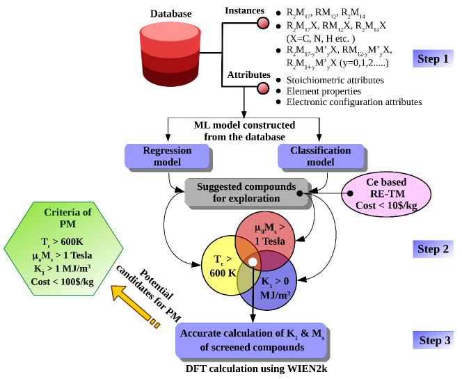
Figure 1: (Color online) Steps of Machine learning combined DFT approach for predictions of properties in Ce₂Fe_17-xCo_xCN permanent magnets.

Permanent magnets are a part of almost all the most important technologies, starting from acoustic transducers, motors and generators, magnetic field and imaging systems to more recent technologies like computer hard disk drives, medical equipment, magneto-mechanics etc.PM The search for efficient permanent magnets is thus everlasting. In this connection, the family of rare-earth (RE) and 3d transition metal (TM) based intermetallics has evolved over last 50 years or so, and has transformed the landscape of permanent magnets.RE-TM ; sun Two most prominent examples of RE-TM permanent magnets, that are currently in commercial production, together with hard magnetic ferrites, are SmCo₅, and NdFe₁₄B.

While SmCo₅ and NdFe₁₄B provide reasonably good solutions, keeping in mind the resource criticality of RE elements like Nd and Sm, a significant amount of effort has been put forward in search of new permanent magnets without critical RE elements or with less content of those. The idea is to optimize the price-to-performance ratio.RE-TM This has lead to two routes, (a) search for potential magnets devoid of rare-earth elements,RE-free and (b) designing of rare-earth lean intermetallics using abundant RE elements such as La and Ce instead of Sm and Nd.acta ; Pandey ; Ce As stressed by Coey,coey2012 the demand in hand is to seek for new, low-cost magnets with maximum energy product bridging the ferrites and presently used RE magnets. Following the route (b), cheap, new ternary and quartnary RE-lean RE-TM intermetallics need to be explored, as binaries have been well explored. In parallel, Co being expensive, it may be worthwhile to focus on intermetallic compounds containing Fe.

Starting from the simplest binary RE-TM structure of CaCu₅, by replacing $n$ out of $m$ RE (R) sites with a pair of TM (M) sites, R_m-nM_5m+2n structures are obtained. This can give rise to several possible binary structures of different chemical compositions, listed in order of RE-leanness; RM₁₃ (7.1$\%$), RM₁₂ (7.7$\%$), R₂M₁₇ (10.5$\%$), R₂M₁₄ (12.5 $\%$), RM₅ (16.7$\%$), R₆M₂₃ (20.7 $\%$), R₂M₇ (22.2 $\%$), RM₃ (25 $\%$), RM₂ (33 $\%$) etc. Judging by the rare-earth content, 1:13, 1:12, 2:17, 2:14 compounds may form examples of rare-earth lean materials. It is desirable to modify the known binary compounds containing low cost RE’s belonging to these families to achieve best possible intrinsic magnetic properties, namely (i) high spontaneous or saturation magnetization ($\mu_{0}$M_s), at least around 1T, (ii) a Curie temperature (T_c) high enough for the contemplated devise use, 600 K or above, and (iii) a mechanism for creating sufficiently high easy-axis coercivity (K_u). The synthesis and optimization of properties of real materials in experiment is both time-consuming and costly, being mostly based on trial and error. Computational approach in this connection is of natural interest to screen compounds, before they can be suggested and tested in laboratory. Typical computational approaches in this regard are based on density functional theory (DFT) calculations. A detailed calculation estimating all required magnetic properties, i.e M_s, T_c, K_u from first-principles is expensive and also not devoid of shortcomings. For example, estimation of T_c relies on parametrization of DFT or supplemented $U$ corrected theory of DFT+$U$ total energies to construct spin Hamiltonian and solution of spin Hamiltonian by mean field or Monte Carlo method. While this approach would work for localized insulators, its application to metallic systems with itinerant magnetism is questionable, as it fails even for elemental metals like Fe, Co and Ni.fe-co-ni A more reasonable approach of DFT+dynamical mean field (DMFT)dmft is significantly more expensive. An alternative approach would be to use machine learning (ML) technique based on a suitable training dataset. This approach has been used for RE-TM permanent magnets based on DFT calculated magnetic properties database of M_s and K_u.acta ; srep Creation of database based on calculations, even with high throughput calculations is expensive, and relies on the approximations of the theory. It would be far more desirable to built a dataset based on experimental results, and then train the ML algorithm based on that. However, the size and availability of the experimental data in required format can be a concern. Focusing on the available experimental data on RE lean intermetallics, the set of T_c is largest, followed by that for K_u, and M_s. While the quantitative values of T_c’s in Kelvin or degree Celsius are available in literature, for magnetocrystalline anisotropy often only the information whether they are easy-axis or easy-plane are available. Similarly, the $\mu_{o}$M_s values are reported either in $\mu_{B}/f.u.$ or in emu/gm or in Tesla, conversion from $\mu_{B}/f.u.$ and emu/gm to Tesla requiring information of the volume and density, which may introduce inaccuracies up to one decimal point. Restricting experimental data to those containing values of K_u, and $\mu_{o}$M_s values in the same format (either Tesla or $\mu_{B}/f.u.$ or emu/gm) reduces the dataset of K_u and M_s significantly, making application of ML questionable. We thus use a two-prong approach, as illustrated in Fig. 1. We first create a database of T_c, M_s and K_u from available experimental data on RE-lean intermetallics, and use ML for prediction of T_c values, for predicting whether $\mu_{0}$M_s satisfies the criteria of being larger than 1 Tesla, and for predicting the sign of K_u. For M_s and K_u, ML thus serves the purpose of initial screening. We next evaluate M_s and the magnetic anisotropy properties based on elaborate DFT calculations. Calculation of the magnetic anisotropy energy (MAE) is challenging due to its extremely small value. However, since the pioneering work of Brooks,brooks several studiesmazin ; smco5 ; Pandey ; durga have shown that $U$ corrected DFT generally reproduces the orientation and the right order of magnitude of the MAE.
We demonstrate applicability of our proposed approach on Ce and Fe based 2:17 RE-TM intermetallics, Ce₂Fe_17-xCo_x compounds ($x$ = 1, $\ldots$, 7). Our choice is based on following criteria, (a) the compounds contain rare earth Ce which is the cheapest one among the RE family having market price of $\sim$ 5 USD/Kg.marketprice The cost of other components Fe, C and N are all $<$ 1 USD/Kg. The price of Co is higher than Fe,marketprice being less abundant metal. The Co:Fe ratio is thus restricted within 0.4. (b) Co substitution in place of Fe has been reportedodkhuu1 ; odkhuu2 to be efficient in simultaneous enhancements of K_u as well as T_c in several TM magnets. This is in sharp contrast to other TM substitutes, such as Ti, Mo, Cr, and V, where magnetic anisotropy as well as T_c are generally suppressed. (c) the search space belongs to 2:17 family, which is the family in which most of the instances in our training set belongs to. (d) this class of compounds is found to be more stable than the well explored 1:12 compounds. (e) for large saturation magnetization it is desirable to use Fe-rich compounds, which is also less expensive compared to Co. (f) although Ce has negative second order Stefan’s factor which favors in-plane MAE, experimental findings support that the nitrogenation and carbonation can switch the MAE from easy plane to easy axis.xu (g) though R₂Fe₁₇ compounds display large magnetization value due to high Fe content, these compounds are disadvantageous as they exhibit low Curie temperature.book Presence of Co, as well as C/N interstitials help in increasing T_c. (h) while magnetic properties of carbo-nitrides are expected to be similar to that of nitrides for sufficiently high concentration of N, carbo-nitride compounds have been proven to show better thermal stability.chen

Our study suggests that Fe-rich Ce₂Fe_17-xCo_xCN compounds may form potential candidate materials for low-cost permanent magnets, satisfying the necessary requirements of a permanent magnet with T_c $>$ 600 K, $\mu_{0}$M_s $>$ 1 Tesla and easy-axis K_u $>$ 1 MJ/m³. The calculated maximal energy product and estimated anisotropy field, which are technologically interesting figures of merit for hard-magnetic materials, turn to be within the reasonable range. Some of the studied compounds may possibly bridge the gap between low maximal energy product and high anisotropy field for SmCo₅ and vice versa for Nd₂Fe₁₄B.

II Machine learning approach

II.1 Database construction & Training of Model

Aiming to search new candidates for permanent magnets we use supervised machine learning (ML) algorithm which helps us to screen compounds with high T_c (T_c $\gtrsim$ 600 K), high M_s ($\mu_{0}$M${}_{s}>$ 1 Tesla), and easy axis anisotropy (K_u $>$ 0) among the huge number of possible candidates of unexplored RE-TM intermetallics. The first step of any ML algorithm is to construct a dataset. We construct three datasets of existing RE-TM compounds for T_c, M_s and K_u separately using the following sources: ICSD,icsd the handbook of magnetic materials,mm the book of magnetism and magnetic materials,mmm and other relevant references.debref1 ; debref2 ; debref3 ; debref4 ; debref5 ; debref6 ; debref7 ; debref8 ; debref ; debref9 ; debref10 ; debref11 ; debref12 ; debref13 ; debref14 ; debref15 ; k1-1 ; k1-2 ; k1-3 ; k1-5 ; k1-6 ; k1-7 ; k1-9 ; k1-10 ; k1-11 ; k1-12 ; k1-13 ; k1-14 ; k1-15 ; k1-16 ; k1-19 ; k1-20 ; k1-21 ; xu ; k1-23 ; k1-24 ; k1-25 ; k1-26 ; k1-27 ; k1-28 ; k1-29 ; k1-31 ; k1-32 ; k1-33 ; k1-34 ; k1-35 ; chen ; k1-37 ; k1-38 ; k1-39 ; n1 ; n2 ; n3 ; n4 ; n5 ; n6 The datasets are presented as supplementary materials (SM)suppl as easy reference for future users. To construct the database of rare-earth lean compounds, RE percentage in the intermetallic compounds is restricted to $14\%$ which includes the four different binary RE-TM combinations namely RM₁₂, RM₁₃, R₂M₁₇ and R₂M₁₄ along with their interstitial and derived compounds. We discard RM₁₃ from the dataset as only few candidates are available from this series with known experimental T_c, M_s and K_u.

We list a total of 565 compounds with reported experimental T_c, among which majority of the compounds (about $55\%$) belong to R₂M₁₇ series. The minimum contribution to the dataset comes from R₂M₁₄ (about $10\%$) family. The highest T_c in the dataset belongs to R₂M₁₇ class of compounds namely Lu₂Co₁₇ debref1 with T${}_{c}\sim$ 1203 K and the compound with lowest T_c is NdCo_7.2Mn_4.8 ($\sim$ 120 K),mm a member from RM₁₂ family. In the dataset all three compositions with RE to TM ratio 2:17, 2:14 and 1:12 show a large variation in T_c having the difference between maximum and minimum values as 1051, 775 and 991 K respectively. There exists few compounds in the dataset with more than one reported value of T_c. For example T_c of SmFe₁₀Mo₂ has been reported with two different values of 421 Ksmfe10mo21 and 483 K.smfe19mo22 There are other examples of such multiple T_c.mtc1 ; mtc2 ; mtc3 ; mtc4 ; mtc5 The quality of the sample, their growth conditions, coexistence of compounds in two or multiple phases and accuracy of the measurements may lead to the multiple values of T_c reported for a particular compound. In such cases, we consistently consider the largest among the reported values of T_c. Notably in majority of cases we find little variation in reported values of T_c ($\sim$ 20-50 K).

Attribute Type	Attribute	Notation	Value range
Stoichiometric	CW absolute deviation	$<\Delta Z>$	1.70-16.74
	of atomic no.
	CW av. of	$<Z_{TM}>$	10-33.30
	atomic no. of TM
	CW av. of	$<Z_{LE}>$	0-9.79
	atomic no. of LE
	CW av. Z	$<Z>$	21.08-37.71
	CW electronegativity	$\Delta\epsilon$	0.61-1.84
	diff. of RE $\&$ TM
	CW RE percentage	$RE\%$	4.76-14.29
	CW TM percentage	$TM\%$	38.46-95.24
	CW LE percentage	$LE\%$	0-53.85
Element	Atomic no. of RE	$Z_{RE}$	58-71
	Presence of	$N_{TM}$	yes/no
	more than one TM
	Presence of LE	$N_{LE}$	yes/no
Electronic	Total no. of f electrons	$f^{n}$	1-28
	Total no. of f electrons	$d^{n}$	30-136

Table 1: List of 13 different attributes with description, notation and range used in the ML algorithm. Here ”CW” stands for ”composition-weighted”.

The dataset of M_s is relatively smaller than T_c, containing only 195 entries. The majority of the compounds in this dataset belong to 2:17 composition similar to the database of T_c. The relatively smaller dimension of M_s dataset is primarily due to fact that experimental reports available for M_s are much less than T_c. Secondly M_s has been mostly reported at room temperature, in some cases at low temperature. To maintain uniformity of the dataset we consider M_s reported at room temperature, resulting in a lesser number of compounds in the M_s dataset.

Reports with quoted values of anisotropy constant are even more rare. Our exhaustive search resulted in only 73 data points. This pushes the dataset size to the limit of ML algorithms, for which predictive capability becomes questionable due to large bias masking the small variance.njp On other hand, if we allow for also experimental data reporting only sign of K_u, this dataset gets expanded to a reasonable size of 258.

After constructing the dataset, we carry out preprocessing of the data, as outlined in Ref.ourml . It comprises of removal of noisy data, outliers and correlated attributes. For details see Appendix.

The next and the most crucial step is to construct a set of simple attributes, which are capable of describing the instances (in this case RE-TM compounds) and then deploy ML algorithm to map them to a target (in this case T_c, M_s and K_u). The attributes considered in this study are summarized in Table. I, which can be divided into three broad categories, namely, stoichiometric attributes, element properties and electronic configuration attributes. The stoichiometric attributes may contain the information of both elemental and compositional properties as suggested by Ward et al.ward This is based on taking compositional weights (CW) of elemental properties.

In the third step, we train different popular machine learning algorithms with the constructed dataset for prediction. We use ML algorithm in three different problems; (a) to predict the compounds with T_c more than 600 K, (b) compounds with $\mu_{0}$M${}_{s}>$ 1 Tesla, and (c) compounds with easy-axis anisotropy. Regression is used in the former case, whereas latter two cases are treated as classification problems. We use five different ML algorithms for regression in case of T_c namely Ridge Regression (RR),RR Kernel Ridge Regression (KRR),KRR Random Forest (RF),RF ; RF1 Support Vector Regression (SVR)SVR and Artificial Neural Network (ANN).ANN The details can be found in Appendix. Out of the five different ML algorithms, it is seen that random forest performs best, which has been also successfully used for prediction of Heusler compounds,heusler half-Hausler compounds,hh double perovskite compounds,ourml half-Heusler semiconductor with low-thermal-conductivity,half-heusler zeolite crystal structure classificationzeolite etc. Results presented in the following are based on random forest method.

II.2 Model evaluation

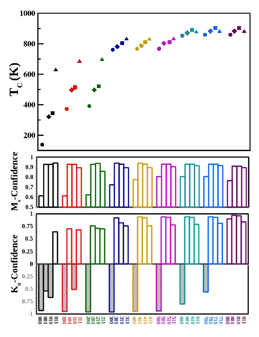
Figure 2: (Color online) ML predictions of Curie temperature (T_c) from regression model, and saturation magnetization (M_s) and anisotropy constant (K_u) from classification model. The upper (middle/lower) panel shows the results of T_c (M_s/K_u). The exploration set is Ce₂Fe_17-xCo_xC_yN_z where $y$ and $z$ can have values either 0 or 1, and $x$ = 0 $\ldots$ 8, acronymed as $x$$y$$z$. In the top panel, non-interstitial compounds, carbonated, nitrogenated and carbo-nitrogenated compounds are symbolized by circle, diamond, square and upper triangle. Different colors specify compounds with different $x$ values. The middle panel shows the ML prediction confidence for M_s. In the lower panel, ML prediction confidence for K_u is illustrated. Here the upper (lower) half having bars with no-fill (shaded) shows the confidence for the compounds with positive (negative) K_u.

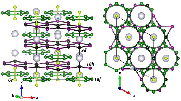
Figure 3: (Color online) Crystal structure of Ce₂Fe_17-xCo_xCN magnets. The Ce, Fe/Co and C/N atoms are shown with large, medium and small balls, respectively. Four transition metal sublattices 9$d$, 18$f$, 18$h$ and 6$c$ are shown in black, green, magenta and yellow colored balls, respectively. Left panel shows the crystal structure viewed with c-axis pointed vertically up and the right panel shows the crystal structure viewed along the c-axis.

The final step is to employ the trained algorithm on yet-to-be synthesized RE-TM compounds, and thus to explore new compositions with targeted properties. We choose Ce₂Fe_17-xCo_xC_yN_z ($y$,$z$ = 0/1; $x$ = 0 $\ldots$ 8) as the exploration set for application of the trained ML algorithm. This results in a set of 36 compounds among which 8 compositions (Ce₂Fe_17-xCo_xCN, $x$ = 1, $\ldots$, 8) have neither been synthesized experimentally nor studied theoretically, to the best of our knowledge. We apply our trained ML algorithms on all of these 36 compounds and the results are summarized in Fig. 2. The top panel of Fig. 2 shows the predicted T_c of all the compounds. It is seen that the nitrogenation or carbonation increases the T_c with respect to their respective parent compound Ce₂Fe_17-xCo_x. Our ML model predicts that the nitrides have higher T_c than that of the carbides. For $x$ $\leq$ 5, the enhancement of T_c is maximum for the compounds where both carbon and nitrogen are present. For $x$ $>$ 5, T_c shows slight decrease compared to only nitrogenated case. It is also noted that the relative rise in T_c in interstitial compounds compared to parent compounds, decays gradually with Co concentration. The increase in T_c varies from $\sim$ 200 K to 10 K as $x$ varies from 0 to 8 for carbides and nitrides whereas introduction of both nitrogen and carbon shows the variation from $\sim$ 310 K to 30 K. Our result reproduces the trend of experimental findings in a qualitative manner. The experimental results for $x$ = 0 (Ce₂Fe₁₇),fuji1992 ; fuji1995 concluded that the enhancement in T_c is highest in presence of both carbon and nitrogenalto93 ; chen93 (T${}_{c}\sim$ 721 K), followed by nitrogenated compoundbuschow90 ; liu91 (T${}_{c}\sim$ 700 K) and lowest for carbonated compoundalto93 ; chen93 (T${}_{c}\sim$ 589 K). Though it is not possible to compare the results quantitatively as the stoichiometry of the experimentally studied carbonated and nitrogenated compounds are not the same as in our exploration dataset, but the overall trend is similar. We also find that our ML model underestimates the T_c of the pure binary compound Ce₂Fe₁₇.book This is expected, as already discussed, our model is less precise for the prediction of low T_c compounds.
Switching to the M_s part, the middle panel of Fig. 2 shows the confidence of classification of compounds with $\mu_{0}$M_s more than 1 T. The confidence value closer to 1 implies that the prediction is viable to be more accurate. All the compounds are classified in favor of forming permanent magnets with $\mu_{0}$M${}_{s}>$1 T. For compounds like Ce₂Fe_17-xCo_x the prediction confidence varies from 0.6 to 0.8 with increasing Co concentration, whereas the carbon and nitride compounds are always classified with high prediction confidence.
The predictions from classification model on K_u is shown in bottom panel of Fig. 2. We find while the anisotropy of Fe_17-xCo_x compounds without interstitial C/N ($x$ = 2, $\ldots$ 7) atoms are predicted to be easy-plane, their carbonated/nitrogenated/carbo-nitrogenated counterparts show easy-axis anisotropy. For pure Fe compounds, apart from carbo-nitrogenated compound, all are predicted to be easy-plane, while for Fe₁₆Co compounds carbonated as well as carbo-nitrogenated compounds are predicted to be easy-axis. This in turn, highlights the effectiveness of Co substitution on making K_u positive. We note the prediction confidence of the carbo-nitrogenated compounds are around 0.75.
On basis of the above ML analysis, we pick up seven yet-to-be synthesized compounds, Ce₂Fe_17-xCo_xCN, $x$ = 1, $\ldots$, 7. This choice is guided by the compounds satisfying T${}_{c}>$ 600 K from regression model, and $\mu_{0}$M${}_{s}>$ 1 Tesla with easy-axis anisotropy from classification models, and being Fe-rich. In following, we describe their crystal structure, and present results of DFT calculated electronic structure, anisotropy properties, and stability properties.

III DFT Calculated Properties of Predicted Compounds

III.1 Crystal Structure

The Ce₂Fe₁₇ compounds crystallize in the rhombohedral Th₂Zn₁₇-type structure (space group R$\bar{3}$m), derived from the CaCu₅-type structure with a pair (dumbbell) of Fe atoms for each third rare earth atom in the basal plane and the substituted layers stacked in the sequence ABCABC $\ldots$. As shown in Fig. 3, the transition metal atoms are divided into four sublattices, 9$d$, 18$f$, 18$h$ and 6$c$, having 3 (9), 6(18), 6 (18), and 2 (6) multiplicity in the one (three) formula unit primitive-rhombohedral (hexagonal) unit cell. The TM atoms occupying the 6$c$ sites, referred as dumbbell sites, form the $\ldots$-TM-TM-RE-RE-$\ldots$ chains running along the c-axis of the hexagonal cell. The 18$f$ TM atoms form a hexagonal layer, which alternates with the hexagonal layer formed by 9$d$ and 18$h$ TM atoms. The 6$c$ TM-TM doumbells pass through the hexagons formed by 18$f$ TM’s. For the interstitial C and N atoms, neutron powder diffraction,neutron EXAFS experiments confirmed that they fill voids of nearly octahedral shape formed by a rectangle of 18$f$ and 18$h$ TM atoms and two RE atoms at opposite corners, which are the 9$e$ sites of Th₂Zn₁₇-type structure, and having the shortest distance from the RE sites among all available interstitial sites. All our calculations are thus carried out with C/N atoms in 9$e$ positions. The RE atoms in 6$c$ position as well as light elements C/N in 9$e$ interstitial sites belong to the same layer as 18$f$ TMs. As the 9$e$ sites are in the same $c$-plane with the RE sites, having RE atoms at neighbors, introduction of interstitials like C and N, is expected to have a profound influence on the the electronic environment of RE atom, thereby altering the magneto-crystalline anisotropy.

Although the R$\bar{3}$m symmetry is lowered upon Co substitution and the spin-orbit coupling (SOC) in the anisotropy calculation, for the ease of identification, we will still use the the notations 9$d$, 18$f$, 18$h$ and 6$c$. Our total energy calculations show that Co preferentially occupy sites in the sequence 9$d$ $>$ 18$h$ $>$ 6$c$ $>$ 18$f$. Out of available 17 TM sites we have considered Co substitution up to 7 sites, which result in Fe-rich phases of compositions Ce₂Fe_17-xCo_xCN with $x$ = 1, 2, $\ldots$, 7. Following the site preference we consider Co atoms in 9$d$ and 18$h$ sites.

We expect the lattice parameters not to change much upon Co substitution, as Fe and Co, being neighboring elements in periodic table, has similar atomic radii. Nevertheless, to check the influence of Co substitution on lattice structure, we optimize the lattice constant and the volume for all $x$ values. Following our expectation, the results show only a marginal decrease in lattice parameter and volume (with a maximum deviation of 1$\%$) upon increasing Co content, in line with the findings by Odkhuu et al.odkhuu2 for 1:12 compounds, and the experimental findings by Xu and Shaheen on 2:17 compounds.xu This minimal change is found to have no appreciable effect on magnetic properties, as explicitly checked on representative compounds with $x$ = 1, 4 and 7. We thus choose the lattice structure as the optimized lattice structure of $x$ = 0 (see Appendix), with lattice constant = 6.59 $\AA$ and angle $\beta$ = 83.3^o of the rhombohedral unit cellkou-cs in subsequent calculations.

III.2 Magnetic Moment and Electronic Structure

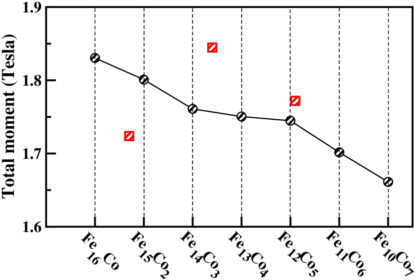
Figure 4: (Color online) Calculated total moment (black circles), $\mu_{0}$M in Tesla plotted for increasing Co concentrations of Ce₂Fe_17-xCo_xCN compounds. Shown are also experimental resultsxu (red, square) for Ce₂Fe_17-xCo_xN_y compounds measured at room temperature. For comparison between T = 0 K calculated moments, and experimental data measured at room temperature, the experimental data has been scaled by a factor of 1.3.

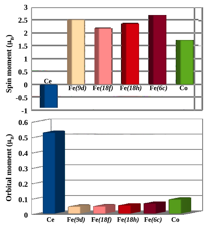
Figure 5: (Color online) Calculated spin (top) and orbital (bottom) moments at Ce, Fe(9$d$), Fe(18$f$), Fe(18$h$), Fe(6$c$) and Co sites in the representative case of Ce₂Fe₁₅Co₂CN compound.

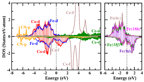
Figure 6: (Color online) Left: Density of states of Ce₂Fe₁₅Co₂CN compound, projected onto Ce $f$ (brown), Ce $d$ (shaded green), Fe $d$ (blue), Co $d$ (shaded red) and CN $p$ (shaded orange) characters. Right: Density of states of Ce₂Fe₁₅Co₂CN compound projected to different Fe $d$’s: Fe(9$d$) (shaded indigo), Fe(18$h$) (magenta), Fe(18$f$) (green) and Fe(6$c$) (brown). The zero of the energy is set at Fermi energy.

In the following we present the DFT results for the magnetic moments and density of states (DOS), as given in GGA+$U$+SOC calculations. The details of the DFT calculations are presented in the Appendix. Importance of application of supplemented Hubbard $U$ on RE sites within LDA or GGA+$U$ formalism is considered as one of the possible means to deal with localized $f$ orbitals of RE ions, and have shown to provide reasonable description.mazin ; smco5 Previous calculations in compounds containing Ce, showed variation of $U$ within 3 eV to 6 eV, keeps the results qualitatively same.Pandey ; eriksson In the following, we present results for $U$ applied on Ce atoms chosen to be 6 eV.

Fig. 4 shows the calculated total magnetic moments of the seven mixed Fe-Co compounds, Ce₂Fe_17-xCo_xCN ($x$ = 1, 2, $\ldots$7). The total magnetic moment shows a decreasing trend with increase of Co concentration, arising from the fact that Co moment is smaller that of Fe. However, it is reassuring to note that even for compound with largest Co concentration, Ce₂Fe₁₀Co₇CN, the calculated moment is more than 1.65 Tesla. This is in agreement with ML prediction, which predicts $\mu_{0}$M_s of all the considered compounds to be larger than 1 Tesla, though it is to be noted the ML predictions are made for room temperature moments while the DFT calculated moments are at T = 0 K. The measured values of total moment in corresponding nitrogenated compounds show good comparison (cf Fig. 4) with our calculated moments. In particular, barring the data on x $\approx$ 2, the other two data point show good matching with the trend of theoretical results. We note that the experimentally determined moments are for Ce₂Fe_17−xCo_xN_y compounds, which contains only N as interstitial atom, and the value of $y$ is not mentioned, which may even vary depending on value of $x$.

Fig. 5 shows the spin and orbital moments projected to Ce, Fe(9$d$), Fe(18$f$), Fe(18$h$), Fe(6$c$) and Co atoms for the representative case of Ce₂Fe₁₅Co₂CN compound. The results for other Co concentrations are similar. In presence of large SOC coupling at Ce site, a substantial orbital moment develops, which is oppositely aligned to its spin moment following Hund’s rule. Considering 3+ nominal valence of Ce, it would be in 4$f^{1}$ state, with S=1/2 and L=3. While the calculated value of Ce spin moment is close to 1 $\mu_{B}$ ($\approx$ 0.95 $\mu_{B}$) in accordance with nominal S=1/2 state, the orbital moment shows significant quenching with a calculated value of about 0.5 $\mu_{B}$. This value of orbital moment is in agreement with DFT calculated values of other Ce containing RE-TM magnets.Pandey ; chauhan The 4$f$ electrons are coupled to 5$d$ electrons at Ce site by intra-atomic exchange interaction, following which their spin moments are aligned in parallel direction. The delocalized 5$d$ electrons at Ce site, hybridize with Fe/Co 3$d$ electrons, favoring antiparallel alignment of Ce and Fe/Co spins, as found in Fig. 5. The spin magnetic moment at Fe sites show a distribution, with Fe at 6$c$ site having largest moment, followed by Fe at 9$d$ and 18$h$ sites while Fe at 18$f$ site shows the lowest moment. We notice that Fe (6$c$) atoms occupying the dumbbell sites, have less connectivity compared to Fe(9$d$), Fe (18$f$) and Fe (18$h$), and thus possess the largest moment, being of most localized character. Among Fe (9$d$), Fe(18$f$), Fe(18$h$) sites Fe (18$f$) has smallest moment, driven by the fact that interstitial C and N atoms are in same plane as Fe (18$f$) causing enhanced $d$-$p$ hybridization, and reduction in moment. These spin moments though are larger than that of bulk Fe ($\approx$ 2.2 $\mu_{B}$). The orbital moment at Fe sites are tiny ($\approx$ 0.05 $\mu_{B}$). In comparison, Co shows significantly smaller spin moment ($\approx$ 1.7 $\mu_{B}$) and somewhat larger orbital moment ($\approx$ 0.1 $\mu_{B}$), justifying the fall in total moment with increasing concentration of Co.

Fig. 6 shows the density of states of Ce₂Fe₁₅Co₂CN, projected to various orbital characters. The Ce 4$f$ states are all unoccupied in the majority spin channel, partly occupied in the minority spin channel, in accordance with nominal $f^{1}$ occupancy. The RE 4$f$ - TM 3$d$ hybridization through empty RE 5$d$ states is visible, making the spin splitting at Fe and Co sites antiparallel to that of Ce. The C/N $p$ states mostly spanning the energy range -7 eV to -4 eV, show non negligible mixing with Fe $d$, Co $d$ and Ce characters, justifying their role in influencing the magnetic properties. Fe $d$ and Co $d$ states span about the same energy range from -4 eV to 2 eV, with states mostly occupied in the majority spin channel and partially occupied in the minority spin channel, largely accounting for the metallicity of the compound. Spin splitting of Fe $d$ is larger than that of Co, being consistent with larger magnetic moment of Fe compared to Co. Projection to different inequivalent Fe sites (cf right panel of Fig. 6), Fe(9$d$), Fe(18$h$), Fe(18$f$) and Fe(6$c$) shows that Fe(6$c$) belonging to dumbbell pair is distinct from other Fe sites, which also exhibit largest magnetic moment among all Fe’s.

III.3 Magneto-crystalline Anisotropy

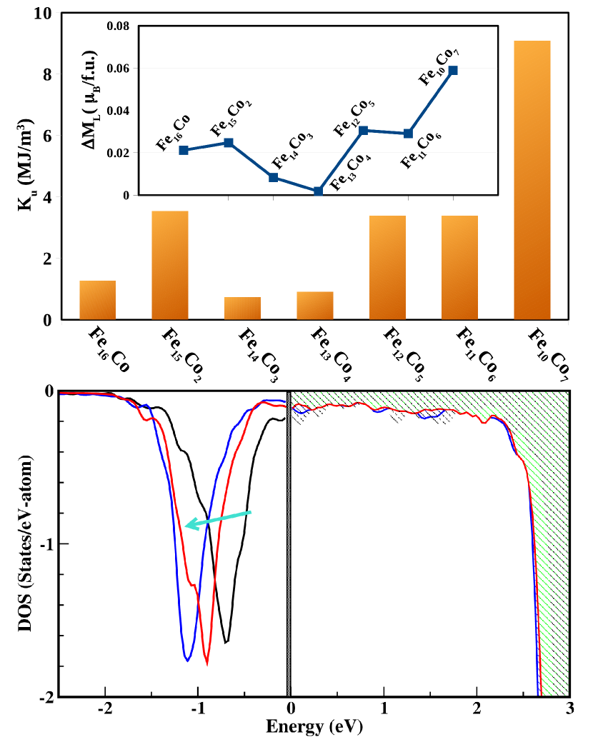
Figure 7: (Color online) Top: Calculated magnetocrytalline anisotropy constant in MJ/m³ plotted for increasing Co concentrations of Ce₂Fe_17-xCo_xCN compounds. The inset shows the anisotropy in orbital moment (see text for details). Bottom: The GGA+$U$+SOC DOS projected to Ce $f$ energy states with magnetization axis pointed along easy-axis, for Ce₂Fe₁₇ (black), Ce₂Fe₁₇CN (red) and Ce₂Fe₁₆CoCN (blue). The zero of the energy is set at Fermi energy, with unoccupied part shown shown as shaded. The arrow indicates the shift in occupied part.

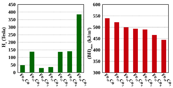
Figure 8: (Color online) Calculated anisotropy field in Tesla (left) and maximal energy product in kJ/m³ (right) plotted for increasing Co concentrations of Ce₂Fe_17-xCo_xCN compounds.

Having an understanding of the basic electronic structure, in terms of magnetic moments and density of states, we next focus on calculation of magneto-crystalline anisotropy constant, K_u, which is a crucial quantity responsible for coercivity in a permanent magnet. MAE defines the energy required for turning the orientation of the magnetic moment under applied field, expressed as $E(\theta)\approx K_{1}sin^{2}\theta+K_{2}sin^{4}\theta+K_{3}sin^{4}\theta cos4\phi$, where K₁, K₂, and K₃ are the magnetic anisotropy constants, $\theta$ is the polar angle between the magnetization vector and the easy axis ($c$-axis), and $\phi$ is the azimuthal angle between the magnetization component projected onto the $ab$ plane and the $a$-axis. In most cases, the higher order term K₃ is relatively small compared with K₁ and K₂. For $\theta$ = $\pi$/2, one may thus write $K_{u}\approx K_{1}+K_{2}$. It’s positive and negative values indicate the easy axis and easy plane anisotropy, respectively. To satisfy the criteria of a good permanent magnet, it should have easy axis anisotropy with value larger than 1 MJ/m³.coey2012 ; RE-TM The MAE in RE-TM arises from two contributions, (i) MAE of the RE sublattice due to strong spin-orbit coupling and crystal field effect and (ii) MAE of TM sublattice. The interplay of the two decides the net sign and magnitude. In particular, in the proposed compounds, presence of Co with significant value of orbital moment, makes the contribution of TM sublattice important. While 2:17 compounds, primarily show easy plane anisotropy, switching to easy axis anisotropy for interstitial compounds have been reported. In particular, upon nitrogenation, easy plane anisotropy has been reported for Ce containing mixed Fe-Co compounds.xu As mentioned already, the interstitial atoms occupy the same plane as the RE atoms, significantly influencing their properties. With predicted high T_c and large saturation moment of our proposed compounds with carbonation and nitrogenation, it remains to be seen whether they would exhibit easy axis anisotropy of reasonable values, as required for a legitimate candidate for permanent magnet. For this purpose, we carry out calculations within GGA+$U$+SOC with magnetization axis pointing along the crystallographic c-axis and perpendicular to it. The importance of application of $U$ on proper description of MAE in terms of its sign and order of magnitude has been stressed upon by several authors.Pandey ; mazin In order to establish our method on calculation of MAE involving small energy difference, we first apply our method to known and well studied case of SmCo₅, with choice of $U$ = 6 eV on Sm, and obtained a MAE value of 24.4 meV/f.u, which agrees well with GGA+$U$+SOC calculated value of 21.6 meV/f.u., reported in literaturemazin as well as experimentally measured values of 13-16 meV/f.u.expt The calculated results for the proposed Ce₂Fe_17-xCo_xCN are shown in top panel of Fig. 7. We found that MAE shows site-dependence on the Co substitution. We consider configurations with Co atoms substituting Fe(9$d$) and Fe(18$h$) sites, configurations involving other substituting sites being energetically much higher. We consider configurations which are energetically close (within 600 K) and calculate the Co-composition dependent MAE using the virtual crystal approximation. Specifically, for $x$ = 1 we consider configurations Co@Fe(9$d$) and Co@Fe(18$h$), the latter being 3.58 meV higher compared to former. Similarly for $x$ = 2, we consider Co@ 2 $\times$ Fe(9$d$) and Co@ 2 $\times$ Fe(18$h$), the latter being 4.43 meV higher compared to former. For $x$ = 3, the configurations considered are, Co@ 2 $\times$ Fe(9$d$)+ Fe(18$h$); Co@ 3 $\times$ Fe(9$d$); Co@Fe(9$d$) + 2 $\times$ Fe(18$h$), the energies being 0 meV (set as zero of energy), 12.37 meV and 47.66 meV, respectively. For $x$ = 4, the configurations considered are, Co@ 2 $\times$ Fe(9$d$) + 2 $\times$ Fe (18$h$); Co@ 3 $\times$ Fe(9$d$) + Fe(18$h$), the energies being 0 meV (set as zero of energy) and 36.5 meV, respectively. For $x$ = 5 , 6 and 7, only one configuration is considered, others being energetically much higher, namely, Co@3 $\times$ Fe(9$d$) + 2 $\times$ Fe(18$h$), Co@3 $\times$ Fe(9$d$)+ 3 $\times$ Fe(18$h$) and Co@3 $\times$ Fe(9$d$) + 4 $\times$ Fe(18$h$), respectively.

Considering spin-orbit effect only on Ce atom, it is found to account for about 60$\%$ of the calculated MAE. We find all the calculated MAE is positive, in good agreement with ML prediction on mixed Fe-Co carbo-nitride compounds. Further MAE values show non-monotonic dependence on Co concentration. Such non-monotonic trend upon varying TM content has been also reported in context of R(Fe_1-xCo_x)₁₁TiZ (R = Y and Ce; Z= H, C, and N)Ce and R-TM systems in general.hal In the inset of top panel of Fig. 7, we show the calculated orbital magnetic anisotropy ($\Delta$M_L) defined as $\Delta$M_L = M_L(a) - M_L(c), as employed in Ref.odkhuu2, , M_L(c) and M_L(a) being the orbital moment along the $c$-axis and $a$-axis, respectively. We find a correlation between $\Delta$M_L and K_u, qualitatively satisfying Bruno’s expressionbruno for itinerant ferromagnets given as, K_u = ($\frac{\xi}{4\mu_{B}}$) $\Delta$ M_L, where $\xi$ is the strength of SOC.

Most of the easy-axis K_u values are found to be larger than 1 MJ/m³, except Fe₁₄Co₃ and Fe₁₃Co₄ for which it is found to be 0.74 and 0.91 MJ/m³, respectively. Few of the concentrations exhibit easy-axis K_u values larger than 2 MJ/m³, e.g. Fe₁₅Co₂ (3.54 MJ/m³), Fe₁₂Co₅ (3.39 MJ/m³), Fe₁₁Co₆ (3.39 MJ/m³), Fe₁₀Co₇ (9.10 MJ/m³), being comparable to Nd₂Fe₁₄B (4.9 MJ/m³).ndfeb

To obtain microscopic understanding of the role of Co substitution and doping by C, N on magnetocrystalline anisotropy, we further calculate the magnetocrystalline anisotropy of Fe-only compounds Ce₂Fe₁₇, Ce₂Fe₁₇C, Ce₂Fe₁₇N and Ce₂Fe₁₇CN. This results in negative K_u values for Ce₂Fe₁₇, and Ce₂Fe₁₇C (-2.12 MJ/m³ and -1.35 MJ/m³), a tiny positive value for Ce₂Fe₁₇N (0.26 MJ/m³) and positive value for co-doped compound Ce₂Fe₁₇CN (1.27 MJ/m³). We further plot the GGA+$U$+SOC density of states (cf bottom panel, Fig. 7) with magnetization axis along c-axis projected to Ce $f$ states for Ce₂Fe₁₇, Ce₂Fe₁₇CN and Ce₂Fe₁₆CoCN, which is expected to reveal the mechanism of uniaxial anisotropy. We find that a lowering of occupied Ce $f$ energy states and increase in band width occur upon introduction of light elements C and N. This gets further helped by substitution of Co, caused by hybridization between Ce $f$ states and Co $d$ and C,N $p$ states. This gain in hybridization energy stabilizes easy-axis magnetization (cf. Ref.jsps, ) as observed experimentally.xu

III.4 Maximal energy product and Anisotropy Field

While, the estimates of K_u and $\mu_{0}$M_s are useful information to access the effectiveness of the suggested materials as permanent magnets, technologically interesting figures of merit of hard magnetic materials, are the maximal energy product (BH)_max and anisotropy field H_a. These can be estimated from the knowledge of $\mu_{0}$M_s and K_u as follows,

$$(BH)_{max}=\frac{(0.9\mu_{0}M_{s})^{2}}{4\mu_{0}}$$

$$H_{a}=\frac{2K_{u}}{\mu_{0}M_{s}}$$

The factor 0.9 in the expression for (BH)_max implies the common assumption that ideally out 10$\%$ of a processed bulk hard magnet consists of non-magnetic phases.non The estimated (BH)_max and H_a is shown in Fig. 8. The (BH)_max value is found to range from 444 to 540 kJ/m³, in comparison to experimentally measured values 516 kJ/m³ and 219 kJ/m³ for Nd₂Fe₁₄Ben and SmCo₅,en respectively. The H_a shows a strong variation with Co concentration, ranging from $\approx$ 1 Tesla to 14 Tesla.ha

We further note that the hardness parameter, defined as $\kappa$ = $\sqrt{\frac{K_{u}}{\mu_{0}M_{s}^{2}}}$, turns out to be greater than 1 for Ce₂Fe₁₅Co₂CN, Ce₂Fe₁₂Co₅CN, Ce₂Fe₁₁Co₆CN, and Ce₂Fe₁₀Co₇CN compounds, employing the calculated T = 0 K values of K_u and M_s.

III.5 Stability

Unlike the other RE-TM magnets like 1:12 compounds, one of the advantage of 2:17 compounds is their stability. Both stable form of Ce₂Fe₁₇ and its Co substituted form have been reported in literature.xu Calculation of formation enthalpies, as given in Ref.odkhuu2, , $E_{form}=\frac{E_{compound}-\sum_{k}N_{k}\epsilon_{k}}{\sum_{k}N_{k}}$, where $N_{k}$ indicate number of different atoms (Ce, Fe, Co, N and C) in the cell, and $\epsilon_{k}$ denote energy/atom of bulk Ce in FCC structure, $\alpha-$ Fe, Co in HCP structure, in molecular nitrogen and C in graphite structure, gives values -0.61 to -0.59 eV/atom for the studied Ce₂Fe_17-xCo_xCN compounds.

A major challenge with interstitial compounds, though, is the nitrogen diffusion.chen It has been further suggested the blockage of nitrogen diffusion by carbon layer is useful in reduction of nitrogen outgassing in carbo-nitrides. In particular, heating up Sm₂Fe₁₇ carbo-nitrides at a constant rate in a differential scanning calorimeter, the onset temperature of nitrogen outgassing was found to be higher by more than 40 K, as compared to nitride counterpart.chen This justifies the choice of carbo-nitrides as our exploration set. To this end, we calculate the vacancy formation energy of the interstitial atoms in our chosen compounds. For this purpose, we calculate the formation energy of the N and/or C vacancy ($\Delta E_{f}$) defined as,

$$\Delta E_{f}=E^{N(C)_{vac}}-E^{pristine}+E_{N(C)}$$

where $E^{N(C)_{vac}}$ and $E^{pristine}$ denote the optimized total energies of compound containing N and/or C vacancy, and vacancy free compound. The internal positions for defect free pristine structure and structures containing nitrogen and/or carbon vacancies are performed keeping the lattice parameters fixed. $E_{N(C)}$ is the energy per N or C atom, which is obtained from calculation of N₂ molecule or graphite. The obtained results for Ce₂Fe_17-xCo_xCN compounds in minimum energy configuration of Co is shown in Table II. The vacancy formation energies show hardly any variation on chosen configuration for a given Co concentration.

	$\Delta E_{f}(CN)$	$\Delta E_{f}(N)$	$\Delta E_{f}(C)$
$x$ = 1	4.32	2.10	0.97
$x$ = 2	3.99	2.09	0.85
$x$ = 3	4.16	2.09	0.88
$x$ = 4	3.98	2.10	0.79
$x$ = 5	3.82	2.07	0.70
$x$ = 6	3.91	2.05	0.72
$x$ = 7	3.78	2.01	0.69

Table 2: Vacancy formation energy for carbon ($\Delta E_{f}(C)$), nitrogen ($\Delta E_{f}(N)$) and nitrogen-carbon ($\Delta E_{f}(CN)$) in eV in Ce₂Fe_17-xCo_xCN compounds.

The vacancy formation energies, listed in Table II, show only small variation between compounds of varying Co concentration, with the general trend $\Delta E_{f}(CN)$ $>$ $\sum$ ($\Delta E_{f}(N)$ + $\Delta E_{f}(C)$). The individual nitrogen vacancy formation energy and carbon vacancy formation energy, are in overall agreement with that found for related compound, SmCaFe₁₇C(N)₃.Pandey The vacancy formation energy for co-doped carbon-nitrogen compounds are found to be enhanced by about 35-40 $\%$ compared to the sum of the individual C and N vacancy formation energies, proving the carbo-nitrogenation co-doping to provide better thermal stability. We also check our results by repeating vacancy formation energy calculations for $x$ = 0 compounds, which however do not show significant difference, suggesting Co doping not having major role in stability, as also indicated by no significant variation of results between $x$ = 1, 2, 3, 4, 5, 6 and 7.

IV Conclusion

Designing alternative solutions for permanent magnets, satisfying the criteria of low-cost, while keeping the magnetic properties comparable to those of permanent magnets in use, is of utmost importance for cost-effective technology. Towards this goal, we use a combined route of machine learning, based on experimental data, and the first-principles calculations. While machine learning has been applied for problem of rare-earth magnets,acta those studies have been based on the dataset created out of high throughput calculations. Being dependent on calculation-based inputs, creation of such database is not only computationally expensive, but also not devoid of approximations of the theory. Our study, to the best of our knowledge, being based on a exhaustive search of experimental data, is first of this kind in context of rare-earth magnets.

While a large volume of experimental data is available with numerical value of T_c, the corresponding dataset with numerical values of M_s and K_u is small. On the other hand, there exists sizable dataset with information of K_u being positive (easy axis) or negative (easy plane), and $\mu_{0}$M_s being larger or smaller than 1 Tesla. We thus employ regression model of machine learning training to make predictions on numerical values of T_c, and classification model to make predictions on sign of K_u, and $\mu_{0}$M_S being larger or smaller than 1 Tesla. We apply the trained machine learning to 2:17 rare-earth transition metal compounds with carbon and nitrogen in interstitials. We choose the compounds to contain abundant rare-earth Ce, and to be Fe-rich to make them cost-effective. Although nitrogenated version of this series has been investigated,xu the systematic study of the carbo-nitride family to the best of our knowledge is unavailable. The machine learning predicts T_c of the chosen carbo-nitride family to be larger than 600 K, $\mu_{0}$M_S $>$ 1 Tesla, and K_u $>$ 0, thereby indicating the possibility of them to become good solutions for cost-effective, permanent magnets. Subsequent first-principles calculations, show T=0 K, $\mu_{0}$M_S to be larger than 1.65 Tesla, and K_u $\gtrsim$ 1 MJ/m³ for the entire family, Ce₂Fe_17-xCo_xCN ($x$ = 1, $\ldots$ 7). Calculated K_u values are found to be comparable to the state-of-art permanent magnet Nd₂Fe₁₄B for Ce₂Fe₁₅Co₂CN, Ce₂Fe₁₂Co₅CN, Ce₂Fe₁₁Co₆CN, and Ce₂Fe₁₀Ce₇CN. This results in two figure of merits for hard magnets, (BH)_max and H_a in range of 444-540 kJ/m³ and $\approx$ 1 - 14 T, respectively.

In spite of good magnetic properties, one of the limitation of practical applications of interstitial 2:17 magnets is the formation of nitrogen/carbon vacancies at high temperature. By calculating the N-(C)-vacancy formation energy, we show that carbo-nitrogenation co-doping enhances the vacancy formation energy significantly, by 35-40 $\%$ compared to sum of individual doping. This is likely to improve the thermal stability at high temperature condition.

Our computational exercise based on exhaustive search of experimental database, should motivate future experimental processes in making high-performance 2:17 interstitial magnets, with cheapest RE element Ce, the most abundant $3d$ metal, Fe and cheap non-metal interstitial dopings like C and N. The estimated price-to-performance based on calculated energy product, and available market pricemarketprice turns out to be 0.03-0.22 USD/J. The enhanced thermal stability of the carbo-nitrides compounds against the vacancy formation of the light elements further boosts the promises of the suggested compounds.

V Acknowledgement

The authors acknowledge the support of DST Nano-mission for the computational facility used in this study.

VI Appendices

VI.1 DFT details

DFT calculations for electronic structure, magnetocrystalline anisotropy are performed using the all-electron density-functional-theory code in full potential linear augmented plane wave (FP-LAPW) basis, as implemented in WIEN2K code.wien2k For expensive structural optimization calculations, the plane wave based calculations, as implemented in Vienna Ab-initio Simulation Package (VASP),vasp are carried out. The exchange-correlation functional is chosen to be generalized-gradient approximation (GGA) of Perdew, Burke, and Ernzerhof.PBE The localized nature of 4$f$ states of Ce is captured through GGA+$U$ calculations,gga+u with choice of $U$ = 6 eV and J_H = 0.8 eV. For light rare earths like Ce the $U$ value was shown to range from 4 eV to 7 eV, without affecting much the physical properties.eriksson The spin-orbit coupling effect at Ce, and TM sites are captured through GGA+$U$+SOC calculations.
For FP-LAPW calculations, APW $+$ lo is used as the basis set, and the spherical harmonics are expanded upto $l=$ 10 and the charge density and potentials are represented upto $l=$ 6. The sphere radii are set at 2.5, 1.9, 2.34, 1.56 and 1.51 bohr for Ce, Fe, Co, N, and C. For good convergence, a RK_max value (the product of the smallest sphere radius and the largest plane-wave expansion wave vector) of 7.0 is used. We set the cutoff between core and valence states at $-$8.0 Ry. The k-space integrations are performed with 112 k-points in irreducible Brillouin zone (BZ), following the report of use of 80 k-points in irreducible BZ in case of SmCo₅ to provide good estimate of MAE.mazin Nevertheless, the convergence of results on k-space mesh is checked by carrying out calculation with 260 k-points.
The structural optimization in plane wave basis is carried out starting with experimental structure of Sm₂Fe₁₇CN, kou-cs replacing Sm with Ce, and relaxing all the internal coordinates until forces on all of the atoms become less than 0.001 eV/Å. Upon moving from Sm 2:17 carbide/nitride interstitial compounds to Ce counterpart, the cell volume changes only nominally by 0.2$\%$ to 0.4$\%$.Pandey For the plane wave calculations, energy cut-off of 600 eV and Monkhorst pack $k$-points mesh of $8\times 8\times 8$ are used.
All the calculations are performed by considering a collinear spin arrangement. The MAE is obtained by calculating the GGA+$U$+SOC total energies of the system, in FP-LAPW basis as K_u = E_a - E_c , where E_a and E_c are the energies for the magnetization oriented along the crystallographic $a$ and $c$ directions, respectively. For accurate estimates of vacancy formation energy, we also use FP-LAPW basis.

VI.2 Data preprocessing in Machine Learning

While constructing the database, we avoid inclusion of noisy data. We do bootstrapping to normalize the data which is followed by removal of outliers with the help of violin plot. A data is removed if it lies outside of Q1-1.5$\times$IQR or Q3+1.5$\times$IQR, where IQR is the interquartile range and Q1, Q2 and Q3 are lower, median and upper quartile respectively. In the next step we identify correlated attributes using Pearson’s correlation coefficient which can be defined as,

$$r=\dfrac{\sum_{i=1}^{i=n}(x_{i}-\bar{x})(y_{i}-\bar{y})}{\sqrt{\sum_{i=1}^{i=n}(x_{i}-\bar{x})^{2}}\sqrt{\sum_{i=1}^{i=n}(y_{i}-\bar{y})^{2}}}$$

Here $n$ is the sample size, $x_{i}$ and $y_{i}$ are sample points and $\bar{x}$ and $\bar{y}$ are the sample means.

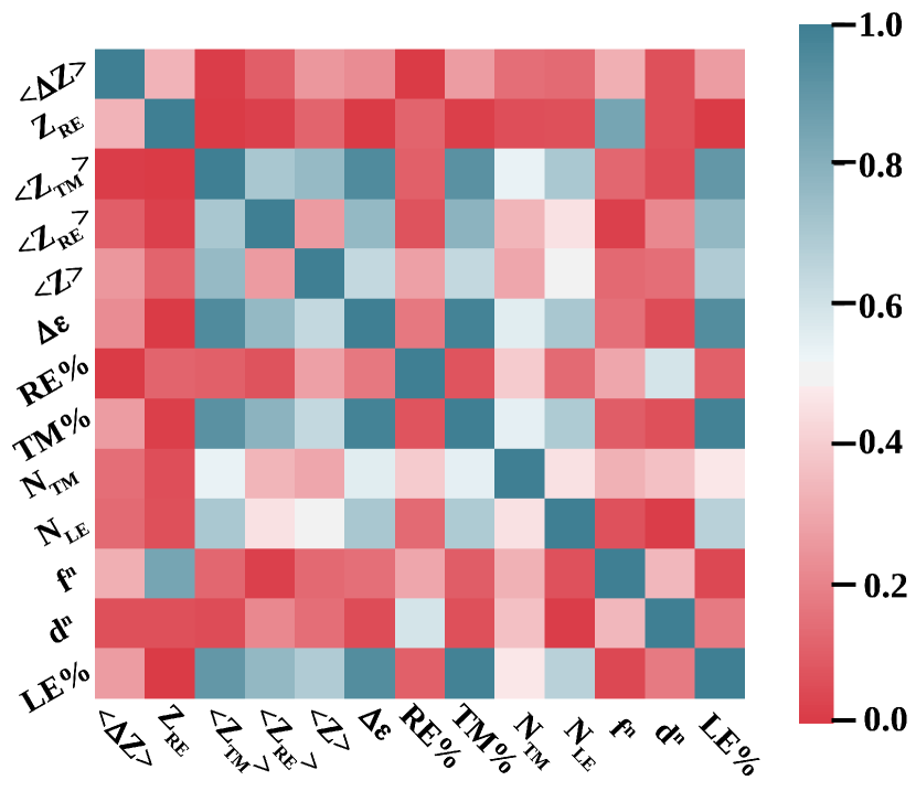
Figure 9: (Color online) Heatmap indicating the correlation between different attributes considered to built ML algorithm. The color code is shown in the side panel. The boxes with red represent weak or no correlation, whereas blue boxes represent strong correlation between the attributes.

The heatmap obtained by using the above mentioned correlation is shown in Fig. 9. The correlation between the attributes is mapped between 0 and 1, considering the absolute values. The highly correlated attributes with correlation greater than 0.75 are as follows:

1. Electronegativity difference between RE and TM ($\Delta\epsilon$) and CW average of atomic no. of TM ($<Z_{TM}>$)

2. CW TM percentage ($TM\%$) and CW average of atomic no. of TM ($<Z_{TM}>$).

3. CW TM percentage ($TM\%$) and Electronegativity difference between RE and TM ($\Delta\epsilon$).

4. Total number of f electrons ($f^{n}$) and Atomic no. of RE ($Z_{RE}$).

5. LE percentage ($LE\%$) and CW average of atomic no. of TM ($<Z_{TM}>$).

6. LE percentage ($LE\%$) and Electronegativity difference between RE and TM ($\Delta\epsilon$).

7. LE percentage ($LE\%$) and CW TM percentage ($TM\%$).

We thus discard $\Delta\epsilon$, $LE\%$, $Z_{RE}$ and $<Z_{TM}>$ from the list of attributes.

VI.3 Model construction for training in ML

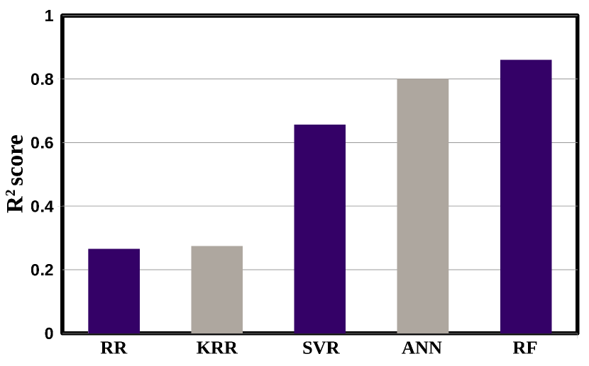
Figure 10: (Color online) Coefficient of determination $R^{2}$ score of five different ML algorithms applied to T_c dataset.

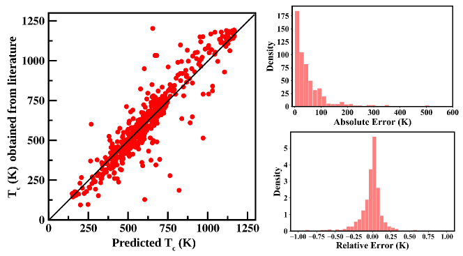
Figure 11: (Color online) Model output from RF algorithm for T_c of RE-TM intermetallics. The left panel shows the comparison of T_c obtained from literature and predicted T_c. The distribution of absolute error between predicted T_c and actual T_c is shown in the upper, right panel, while the lower, right panel presents the distribution of relative error for the compounds with T${}_{c}>$ 600 K.

The performance of a model can be quantified in terms of coefficient of determination which can be expressed as follows:R2

$$R^{2}=1-\dfrac{\sum_{i=1}^{N}[y_{i}-f(x_{i})]^{2}}{\sum_{i=1}^{N}[y_{i}-\mu]^{2}}$$

for predictions ${f(x_{i})}$ and a set of actual values ${y_{i}}$ with mean $\mu$. If the algorithm performs perfectly, $R^{2}$ score is 1. Fig. 10 shows score $R^{2}$ for five different algorithms. RR algorithm circumvents issues in ordinary linear regression like over-fitting or failure in finding unique solution due to multicollinearity. It develops on least square error by adding an extra penalty/regularization term to the loss function of ordinary linear regression. KRR builds on the ridge regression technique by using kernel trick trick so that it can capture the nonlinearity present in the feature space. It can fit a non linear function by learning from a linear function spanned by a kernel which in turn mimics a non-linear function in the original space. SVR originated from support vector machines which are mainly popular in classification problem. It is based on the idea to search a hyperplane plane by minimizing the error which is able to separate two different classes. SVR also uses kernel trick to map the data into a high dimensional feature space and then performs linear regression to fit the data. These three models are based on the same principle of linear regression and SVR is the best form according to our result. $R^{2}$ score is 0.66 for SVR whereas it is found to be poor ($\approx$ 0.25) for other two algorithms.

Apart from these we use two other algorithms, ANN and RF. The model performance scores are satisfactory for both of them. A simple ANN architecture called perceptron implements a processing element or artificial neuron called Threshold Logic Unit (TLU) which can have one or more input(s) and one output. Each input is related to a weight. The TLU calculates the weighted sum of its inputs, applies a step function (generally Heaviside or sign function) to it and outputs the result. A perceptron perceptron is simply a layer of TLUs operating in parallel and connected to all the inputs. Training an ANN model is equivalent to learning each weight factor in an iterative cycle. A more complex system (Multi-Layer Perceptron) can be built by associating additional interconnected layers to the architecture. A well functioning system consists of an input layer, several hidden layers and an output layer. In our case we have one input layer, two hidden layers where rectified linear unit (ReLU)relu is used as activation function along with L2 regularization in the kernel, and an output layer. The constructed ANN model shows 0.80 as $R^{2}$ score.
Random forest is an ensemble method which consists of multiple decision trees. Each tree is built on a portion of entire training data with a subset of total number of attributes. Tree algorithm is based on ’top to bottom’ approach, starting from a root node, it consists of many intermediate nodes and ends at leaf nodes. At each node of a tree a particular attribute classifies the data and helps to grow the tree. The prediction is based on accumulating the results from all such trees, taking ensemble average in case of regression or considering votes from majority trees in case of classification. Such an algorithm can capture the complex and nonlinear interaction between different attributes and can built a robust and sophisticated model. Our random forest consists of 100 trees built by bootstrappedboot sampling of the training set. Each tree allows checking a maximum of $\log_{2}$(number of features) while detecting the best split node. The quality of such a split is measured by using mean squared error (Gini index) in regression (classification). The model efficiency is calculated by running out-of-bag samples down each of the trees. We use ten-fold cross validation to extract the hyper-parameter and to construct the best model.
Fig. 11 shows the result of the best regression model using RF algorithm in case of T_c. The plot in the left panel shows the predicted T_c versus T_c obtained from experiments. The determination score $R^{2}$ is high enough (0.86), indicating a good agreement between the predicted T_c and experimentally reported T_c. The mean absolute error in this model is 60 K. Additionally we evaluate absolute error and relative error for the compounds with T${}_{c}>$ 600 K (cf Fig. 11, right panel). This analysis helps to determine the model performance for the compounds with T${}_{c}>$ 600 K as we are interested to predict new RE-TM intermetallics with high T_c. The distribution of absolute error shows that for the most of the compounds ($\approx$ 85$\%$) the absolute error is less than 100 K. For 65$\%$ of the predicted cases, the absolute error is less than 50 K. We also check the absolute error for the compounds with T${}_{c}<$ 300 K (not included in the figure). In this case our model predicts $\approx$ 76$\%$ compounds with absolute error less than 100 K and 50$\%$ instances are predicted with absolute error of 50 K. This observation prompts us to conclude that though the model prediction is in general good, it is less accurate for low T_c compounds compared to high T_c compounds. The distribution of relative error, expressed as $\epsilon_{rel}$ = (T${}_{c}^{exp}$ -T${}_{c}^{predicted}$)/T${}_{c}^{exp}$, provides further support to this statement, which is shown in bottom, right panel of Fig. 11. The relative error distribution appears Gaussian like with slight asymmetry about the mean position. The relative error is less in the right side of the mean position than the left side suggesting the prediction of T_c suffers less overestimation than underestimation. As found, only 1$\%$ of the instances are having $\epsilon_{rel}$ $>$ 50$\%$, 3$\%$ of the instances have 50$\%$ $>$ $\epsilon_{rel}$ $>$ 30$\%$ and 2$\%$ instances have 30$\%>$ $\epsilon_{rel}>$ 25$\%$, most cases having tiny values of $\epsilon_{rel}$. This gives us confidence in accuracy of the predicted T_c for compounds with T_cs exceeding 600 K.

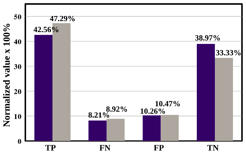
Figure 12: (Color online) Normalized confusion matrix for $\mu_{0}$M_s(violet) and K_u(grey) classification using 10-fold cross-validation. Here positive (negative) class represents either compounds with $\mu_{0}$M${}_{s}>(<)$ 1T, or compounds with uniaxial anisotropy i.e K${}_{u}>(<)$ 0 MJ/m³. True positive/negative or TP/TN are the compounds where their classes are predicted correctly. Whereas false positive (FP) and false negative (FN) are the off-diagonal terms of the matrix where the classes are incorrectly classified.

Turning to M_s, we use random forest algorithm to classify high M_s from low M_s compounds. The best model by performing 10-fold cross validation is built up with 81.53$\%$ accuracy. The resultant confusion matrix is shown in Fig. 12. For classification problem, F1 score determines the balance between precision and recall. In this case F1 score 82.2$\%$ indicates good anticipation with slight favour towards the prediction of compounds with high M_s ($\mu_{0}$M_s $>$ 1) (83.8$\%$) compared to the compounds with low M_s ($\mu_{0}$M_s $<$ 1) (79.2$\%$).
Similar to M_s, we use random forest algorithm for K_u, to classify positive K_u from negative K_u compounds. The best model by performing 10-fold cross validation, in this case, is built up with 80.62$\%$ accuracy Like M_s, in this case F1 score for positive K_u is 83$\%$ and for negative is K_u 77.5$\%$ suggesting slight preference of classification towards positive K_u which is also captured in the plot of confusion matrix as shown in Fig. 12.

References

- (1) K. Buschow, Rep. Prog. Phys. 54 1123 (1991).
- (2) J. M. D. Coey, IEEE Trans. Magn. 47, 4671 (2011).
- (3) Hong Sun, Y. Otani and J.M.D. Coey, Magnetism and Magnetic Materials 104-107 1439-1440 (1992).
- (4) A. Vishina, O. Y. Vekilova, T. Björkman, A. Bergman, H. C. Herper, O. Eriksson, Phys. Rev. B 101, 094407 (2020).
- (5) J. J. Möller, W. Körner, G. Krugel, D. F. Urban, Acta Materialia 153, 53 (2018).
- (6) T. Pandey, M-H. Du and D. S. Parker, Phys. Rev. Appl. 9 034002 (2018).
- (7) L. Ke and D. D. Johnson, Phys. Rev. B 94, 024423 (2016).
- (8) J. M. D. Coey, Scr. Mater. 67, 524 (2012).
- (9) S. V. Halilov, H. Eschrig, A. Y. Perlov, P. M. Oppeneer, Phys. Rev. B 58, 293 (1998).
- (10) A. Georges, G. Kotliar, W. Krauth, and M. J. Rozenberg, Rev. Mod. Phys. 68, 13 (1996).
- (11) W. Körner, G. Krugel, C. Elsässer, Sci. Rep. 6 24686 92016).
- (12) H. Brooks, Phys. Rev. 58 909 (1940).
- (13) P. Larson, I. I. Mazin and D. A. Papaconstantopoulos, Phys. Rev. B 67 214405 (2003)
- (14) S. Yehia, S. H. Aly, A. E. Aly, Computational Materials Science 41 482 (2008).
- (15) H. Ucar, R. Choudhary, D. Paudyal, J. Magn. Magn. Mater, 496 165902 (2020).
- (16) https://en.wikipedia.org/wiki/Prices-of-chemical-elements; J.M.D.Coey Engineering 6, 119 (2020).
- (17) D. Odkhuu, and S. C. Hong, Phys. Rev. Appl. 11, 054085 (2019).
- (18) D. Odkhuu, T. Ochirkhuyag, S. C. Hong, Phys. Rev. Appl. 13, 054076 (2020).
- (19) Xie Xu and S. A. Shaheen, Journal of Applied Physics 73, 5896 (1993).
- (20) H. Fujii, H. Sun. (1995). Chapter 3 Interstitially modified intermetallics of rare earth and 3D elements. Handbook of Magnetic Materials, 303-404.
- (21) X. Chen, Z. Altounian and D. H. Ryan, J. Magn. Magn. Mater. 125 169 (1993).
- (22) https://icsd.nist.gov/guide.html
- (23) K.H.J. Buschow, Handbook of Magnetic Materials, Volumes 6 9 (Elsevier, 1991-1995).
- (24) J. M. D. Coey, Magnetism and Magnetic Materials (Cambridge University Press, 2010)
- (25) Shiqiang Liu, Chin. Phys. B 28, 017501 (2019).
- (26) S. R. Mishra, Gary J. Long, O. A. Pringle, D. P. Middleton, Z. Hu et al., J. Appl. Phys. 79, 3145 (1996).
- (27) H. Klesnar, K. Hiebl and P. Rogl, Journal of the Less-Common Metals 154, 217 (1989).
- (28) R. Guetari, R. Bez, A. Belhadj, K. Zehani, A. Bezergheanu, N. Mliki, L. Bessais, C.B. Cizmas, Journal of Alloys and Compounds 588, 64 (2014).
- (29) Y. Otani, D. P. F. Hurley, Hong Sun, and J. M. D. Coey, Journal of Applied Physics 69, 5584 (1991).
- (30) M. Merches, W.E. Wallace and R.S. Craig, Journal of Magnetism and Magnetic Materials 24, 97 (1981).
- (31) F. Pourarian, R. Obermyer, Y. Zheng, S. G. Sankar, and W. E. Wallace, Journal of Applied Physics 73, 6272 (1993).
- (32) F. Weitzer, H. Klesnar, K. Hiebl, and P. Rogl, J. Appl. Phys. 67, 2544 (1990).
- (33) X.P. Zhong, R.J. Radwanski, F.R. de Boer, T.H. Jacobs and K.H.J. Buschow, Journal of Magnetism and Magnetic Materials 86, 333 (1990).
- (34) A. T. Pedziwiatr and W. E. Wallace, Journal of Applied Physics 61, 3439 (1987).
- (35) R. van Mens, Journal of Magnetism and Magnetic Materials 61, 24 (1986).
- (36) Hu Bo-Ping and J. M. D. Coey, Journal of the Less-Common Metals 142, 295 (1988).
- (37) H. Y. Chen, S. G. Sankar, and W. E. Wallace, Journal of Applied Physics 63, 3969 (1988).
- (38) M. Juczyk and W. E. Wallace, Journal of Magnetism and Magnetic Materials 59, 182 (1986).
- (39) Y.G. Xiao, G.H. Rao, Q. Zhang, G.Y. Liu, Y. Zhang, J.K. Liang, Journal of Alloys and Compounds 407, 1 (2006).
- (40) E. Girt, M. Guillot, I. P. Swainson, Kannan M. Krishnan, Z. Altounian, and G. Thomas, Journal of Applied Physics 87, 5323 (2000).
- (41) Wolfgang Körner, Georg Krugel, and Christian Elsässer, Sci. Rep 6, 24686 (2016).
- (42) A.M. Schönhöbel et al., Journal of Alloys and Compounds 786, 969-974 (2019).
- (43) Y.Z. Wang et al., Journal of Magnetism and Magnetic Materials 104-107, 1132-1134 (1992).
- (44) E.P Wohlfarth and K.H.J. Buschow, Handbook of Magnetic Materials, Vol-4 (Elsevier, 1988).
- (45) Y.Z. Wang et al., Journal of Applied Physics 73, 6251 (1993).
- (46) D. P. F. Hurley and J M D Coey, J. Phys. Condens. Matter 4, 5573 (1992).
- (47) Yosuke Harashima, Kiyoyuki Terakura, Hiori Kino, Shoji Ishibashi, and Takashi Miyake, Phys. Rev. B 92, 184426 (2015).
- (48) Y.G. Xiao, G.H. Rao, Q. Zhang, J. Luo, G.Y. Liu, Y. Zhang, and J.K. Liang, Physica B 369, 56 (2005).
- (49) V.K. Sinha, S.F. Cheng, W.E. Wallace, and S.G. Sankar, Journal of Magnetism and Magnetic Materials 81, 227-233 (1989).
- (50) M. Jurczyk, Journal of Magnetism and Magnetic Materials 89, L5-L7 (1990).
- (51) M. Katter, J. Wecker, C. Kuhrt, L. Schultz, X.C. Kou, and R. Grössinger, Journal of Magnetism and Magnetic Materials 111, 293-300 (1992).
- (52) M. Jurczyk and W.E. Wallace, Journal of Magnetism and Magnetic Materials 59, L182-L184 (1986).
- (53) Yang Fu-ming, Li Qing-an, Zhao Ru-wen, Kuang Jian-ping, F. R. de Boer, J. P. Liu, K. V. Rao, G. Nicolaides, and K. H. J. Buschow, Journal of Alloys and Compounds 177, 93 (1991).
- (54) Bao-gen Shen, Fang-wei Wang, Lin-shu Kong, Lei Cao, and Hui-qun Guo, Journal of Magnetism and Magnetic Materials 127, L267-L272 (1993).
- (55) X. C. Kou, T. S. Zhao, R. Grössinger, and F. R. de Boer, Phys. Rev. B 46, 6225 (1992).
- (56) Zhi-gang Sun et al, J. Phys. Condens. Matter 12, 2495 (2000).
- (57) Z.X. Tang, E.W. Singleton, and G.C. Hadjipanayis, IEEE Trans. on Magn., 28, 5 (1992).
- (58) C.H. de Groot, K.H.J. Buschow, and F.R. de Boer, Physica B 229, 213-216 (1997).
- (59) L. Zhang, D.C. Zeng, Y.N. Liang, J.C.P. Klaasse, E. Bruck, Z.Y. Liu, F.R. de Boer, and K.H.J. Buschow, Journal of Magnetism and Magnetic Materials 214, 31-36 (2000).
- (60) Bing Liang, Bao-gen Shen, Fang-wei Wang, Tong-yun Zhao, Zhao-hua Cheng, Shao-ying Zhang, Hua-yang Gong, and Wen-shan Zhan, Journal of Applied Physics 82, 3452 (1997).
- (61) Zhi-gang Sun, Shao-ying Zhang, Hong-wei Zhang, and Bao-gen Shen, Journal of Alloys and Compounds 322, 69–73 (2001).
- (62) Lin Qin, Sun Yunxi, Lan Jian, Lu Shizhong, and Jiang Hongwei, Chinese Phys. Lett. 8 , No. 5 , 267 (1991).
- (63) Jing-Yun Wang, Bao-Gen Shen, Shao-Ying Zhang, Wen-Shan Zhan, and Li-Gang Zhang, Journal of Applied Physics 87, 427 (2000).
- (64) O. Isnard, and M. Guillot, Journal of Applied Physics 87, 5326 (2000).
- (65) Zhi-gang Sun, Hong-wei Zhang, Shao-ying Zhang, and Bao-gen Shen, Physica B 305, 127–134 (2001).
- (66) M.V. Satyanarayana, H. Fujii, and W.E. Wallace, Journal of Magnetism and Magnetic Materials 40, 241-246 (1984).
- (67) Zhi-gang Sun, Hong-wei Zhang, Shao-ying Zhang, Jing-yun Wang, and Bao-gen Shen, J. Phys. D: Appl. Phys. 33, 485–491 (2000).
- (68) Zhi-gang Sun, Hong-wei Zhang, Shao-ying Zhang, Jing-yun Wang, and Bao-gen Shen, Journal of Applied Physics 87, 8666 (2000).
- (69) E. A. Tereshina, H. Drulis, Y. Skourski, and I. S. Tereshina, Phys. Rev. B 87, 214425 (2013).
- (70) Yingchang Yang, Qi Pan, Xiaodong Zhang, and Senlin Ge, J. Appl. Phys. 72, 2989 (1992).
- (71) Z Altounian, Xu Bo Liu, and Er Girt, J. Phys. Condens. Matter 15, 3315–3322 (2003).
- (72) Linshu Kong, Jiabin Yao, Minghou Zhang, and Yingchang Yang, Journal of Applied Physics 70, 6154 (1991).
- (73) O. Isnard, S. Miraglia, J.L. Soubeyroux, D. Fruchart, and p. L’Heritier, Journal of Magnetism and Magnetic Materials 137, 151-156 (1994).
- (74) D. P. Middleton, S. R. Mishra, Gary J. Long, O. A. Pringle, Z. Hu, W. B. Yelon, F. Grandjean, and K. H. J.Buschow, Journal of Applied Physics 78, 5568 (1995).
- (75) T. Pandey and David S. Parker, Sci Rep 8, 3601 (2018).
- (76) H. Luo, Z. Hu, W. B. Yelon, S. R. Mishra, G. J. Long, O. A. Pringle, D. P. Middleton, and K. H. J. Buschow, Journal of Applied Physics 79, 6318 (1996).
- (77) O. Isnard, S. Miraglia, D. Fruchart, j. Deportes, and P. L’Heritier, Journal of Magnetism and Magnetic Materials 131, 76-82 (1994).
- (78) A.V. Andreev, D. Rafaja, J. Kamarad, Z. Arnold, Y. Homma, Y. Shiokawa, Journal of Alloys and Compounds 383, 40–44 (2004).
- (79) The supplementary materials contain the three datasets for Tc, Ms and Ku.
- (80) V. Psycharis, M. Anagnostou, C. Christides, and D. Niarchos, Journal of Applied Physics 70, 6122 (1991).
- (81) K. Ohashi, Y. Tawara, R. Osugi, and M. Shimao, Journal of Applied Physics 64, 5714 (1988).
- (82) Satoshi Hirosawa, Yutaka Matsuura, Hitoshi Yamamoto, Setsuo Fujimura, Masato Sagawa et al,J. Appl. Phys. 59, 873 (1986).
- (83) C. Abache and H. Oesterreicher,J. Appl. Phys. 57, 4112 (1985).
- (84) Z. X. Tang, G. C. Hadjipanayis and V. Papaefthymiou, Journal of Alloys and Compounds 194, 87 (1993).
- (85) Y. Z. Wang, B. P. Hu, X. L. Rao, G. C. Liu, L. Yin, W. Y. Lai, W. Gong, and G. C. Hadjipanayis, Journal of Applied Physics 73, 6251 (1993).
- (86) M. Anagnostou, C. Christides and D. Niarchos, Solid State Communications, 78, 681 (1991).
- (87) Y. Zhang and C. Ling, npj Computational Materials 4, 25 (2018).
- (88) Anita Halder, Aishwaryo Ghosh, and Tanusri Saha Dasgupta, Phys. Rev. Materials 3, 084418 (2019).
- (89) L. Ward, A. Agrawal, A. Choudhary, and C. Wolverton, npj Comp. Mat. 2, 16028 (2016).
- (90) Wessel N. van Wieringen, Lecture notes on ridge regression, 2020, arXiv:1509.09169v5.
- (91) Vladimir Vovk, Kernel ridge regression, Empirical Inference, Springer Berlin Heidelberg, 2013, ISBN 9783642411366.
- (92) Leo. Breiman, Random forests, Machine learning 45.1,5-32 (2001).
- (93) Andy Liaw, and Matthew Wiener, ”Classification and regression by randomForest.”, R news 2.3, 18-22 (2002).
- (94) Harris Drucker, CJC Burges, Linda Kaufman, Alex J. Smola, and Vladimir Vapnik, Support vector regression machines, Advances in neural information processing systems, pp. 155-161, 1997.
- (95) Mohamad Hassoun, Fundamentals of artificial neural networks, MIT press, 1995, ISBN 9780262514675.
- (96) Anton O. Oliynyk, Erin Antono, Taylor D. Sparks, Leila Ghadbeigi, Michael W. Gaultois, Bryce Meredig and Arthur Mar ,Chem. Mater. 28, 7324 (2016).
- (97) Fleur Legrain, Jesús Carrete, Ambroise van Roekeghem, Georg K.H. Madsen and Natalio Mingo, J. Phys. Chem. B 122, 625 (2018).
- (98) Jesús Carrete, Wu Li, and Natalio Mingo, Shidong Wang, and Stefano Curtarolo, Phys. Rev. X 4, 011019 (2014).
- (99) D. Andrew Carr, Mohammed Lach-hab, Shujiang Yang, Iosif I. Vaisman, Estela Blaisten-Barojas, Microporous and Mesoporous Materials 117, 339 (2009).
- (100) Fujii, H., K. Tatami, M. Akayama and K.Yamamoto, 1992a, in: Proc. 6th Int. Conf. on Ferrites, ICF6, Tokyo and Kyoto, Japan (The Japan Society of Powder and Powder Metallurgy, Tokyo) p. 1081.
- (101) Fujii, H., M. Akayama, K. Nakao and K. Tatami, J. Alloys Comp. 219, 10 (1995).
- (102) Altounian, Z., X. Chen, L.X. Liao, D.H. Ryan and J.O. StrOm-Olsen, J. Appl. Phys. 73, 6017 (1993).
- (103) Chen, X., Z. Altounian and D.H. Ryan, J. Magn. Magn. Mater. 125, 169 (1993).
- (104) Buschow, K.H.J., T.H. Jacobs and W. Coene, IEEE Trans. Magn. MAG-26, 1364 (1990).
- (105) Liu, J.P., K. Bakker, ER. de Boer, T.H. Jacobs, D.B. de Mooij and K.H.J. Buschow, J. Less-Common Met. 170, 109 (1991).
- (106) W.G. Haije, T. H. Jacobs and K. H. J Buschow, J. Less-Common Met. 163 353 (1990); T. W. Capehart, R.K. Misra and F.E. Pickerton, App. Phys. Lett. 58 1395 (1991).
- (107) X. C. Kou, R. Grossinger, M. Katter, J. Wecker, L. Schultz, T. H. Jacobs, K. H. J Buschow, Journal of Applied Physics, 70, 2272(1991).
- (108) I.L.M. Locht, Y.O. Kvashnin, D.C.M. Rodrigues, M. Pereiro, A. Bergman, L. Bergqvist, A.I. Lichtenstein, M.I. Katsnelson, A. Delin, A.B. Klautau, B. Johansson, I. Di Marco, O. Eriksson, Phys. Rev. B 94, 085137 (2016).
- (109) R. K. Chouhan, A. K. Pathak, D. Paudyal, V.K. Pecharsky, arXiv:806.01990.
- (110) B. Szpunar, Acta Phys. Pol. A 60, 791 (1981); T.-S. Zhao, H.-M. Jin, R. Grossinger, X.-C. Kou, and H.R. Kirchmayr, J. Appl. Phys. 70, 6134 (1991); I.A. Al-Omari, R. Skomski, R.A. Thomas, D. Leslie-Pelecky, and D.J. Sellmyer, IEEE Trans. Magn. MAG-37, 2534 (2001).
- (111) N. Thuy, J. Franse, N. Hong, and T. Hien, J. Phys. Colloques 49, 499 (1988).
- (112) P. Bruno, Phys. Rev. B 39, 865 (1989).
- (113) J. Herbst, Rev. Mod. Phys. 63, 819 (1991).
- (114) T. Miyake and H. Akai, J. Phys. Soc. Jpn 87, 041009 (2018).
- (115) Y. Hirayama, Y. Takahashi, S. Hirosawa, K. Hono, Scripta Mater. 95, 70, (2015).
- (116) K.H.J. Buschow, Concise Encyclopedia of Magnetic and Superconducting Materials, Elsevier, 2005, ISBN 9780080457659.
- (117) J.M.D. Coey, Magnetism and Magnetic Materials, 2010, ISBN 0521816149, https://doi.org/10.1017/CBO9780511845000 arXiv:arXiv:1011.1669v3.
- (118) P. Blaha, K. Schwarz, G. K. H. Madsen, D. Kvasnicka and J. Luitz, WIEN2K, An Augmented Plane Wave + Loca Orbitals Program for Calculating Crystal Properties (Technische Universität Wien, Vienna, 2001).
- (119) G. Kresse and J. Hafner, Phys. Rev. B 47, R558 (1993), G. Kresse and J. Furthmueller, Phys. Rev. B 54, 11169 (1996).
- (120) J. P. Perdew, K. Burke, and M. Ernzerhof, Phys. Rev. Lett. 77, 3865 (1996); 78, 1396(E) (1997).
- (121) A.I. Liechtenstein, V.I. Anisimov, and J. Zaanen, Phys. Rev. B52, R5467 (1995).
- (122) Nico JD Nagelkerke, ”A note on a general definition of the coefficient of determination.”, Biometrika 78.3 ,691-692 (1991).
- (123) Bernhard Schölkopf, ”The kernel trick for distances”, Advances in neural information processing systems, 301-307 (2001).
- (124) Support Vector Regression(SVR), https://icme.hpc.msstate.edu/mediawiki/images/5/55/SVR.pdf
- (125) I. Stephen, ”Perceptron-based learning algorithms.”, IEEE Transactions on neural networks 50.2, 179 (1990).
- (126) Di Wei, Anurag Bhardwaj, and Jianing Wei, Deep Learning Essentials, Packt Publishing, 2018, ISBN 9781785880360.
- (127) Bradley Efron, and Robert J Tibshirani, An Introduction to the Bootstrap, CRC Press, 1994, ISBN 9780412042317.