The effective theory of nuclear scattering for a WIMP of arbitrary spin

Abstract

We introduce a systematic approach to characterize the most general non-relativistic WIMP–nucleus interaction allowed by Galilean invariance for a WIMP of arbitrary spin $j_{\chi}$ in the approximation of one–nucleon currents. Five nucleon currents arise from the nonrelativistic limit of the free nucleon Dirac bilinears. Our procedure consists in (1) organizing the WIMP currents according to the rank of the $2j_{\chi}+1$ irreducible operator products of up to $2j_{\chi}$ WIMP spin vectors, and (2) coupling each of the WIMP currents to each of the five nucleon currents. The transferred momentum $q$ appears to a power fixed by rotational invariance. For a WIMP of spin $j_{\chi}$ we find a basis of 4+20$j_{\chi}$ independent operators that exhaust all the possible operators that drive elastic WIMP–nucleus scattering in the approximation of one–nucleon currents. By comparing our operator basis, which is complete, to the operators already introduced in the literature we show that some of the latter for $j_{\chi}=1$ were not independent and some were missing. We provide explicit formulas for the squared scattering amplitudes in terms of the nuclear response functions, which are available in the literature for most of the targets used in WIMP direct detection experiments.

1 Introduction

In one of its most popular scenarios dark matter (DM) is believed to be composed of Weakly Interacting Massive Particles (WIMPs) with a mass in the GeV-TeV range and weak–type interactions with ordinary matter. Such small but non vanishing interactions can drive WIMP scattering off nuclear targets, and the measurement of the ensuing nuclear recoils in low–background detectors (direct detection, DD) represents the most straightforward way to detect them.

The most popular WIMP candidates are provided by extensions of the Standard Model such as Supersymmetry or Large Extra Dimensions which are in growing tension with the constraints from the Large Hadron Collider (LHC). As a consequence, model-independent approaches have become increasingly popular to interpret DM search experiments [1, 2, 3, 4, 5, 6, 7, 8, 9, 10, 11, 12, 13, 14, 15, 16, 17, 18, 19, 20, 21, 22, 23].

In particular, since the DD process is non–relativistic (NR), on general grounds the WIMP-nucleon interaction can be parameterized with an effective Hamiltonian ${\bf\mathcal{H}}$ that complies with Galilean symmetry. The effective Hamiltonian ${\bf\mathcal{H}}$ to zero-th order in the WIMP-nucleon relative velocity $\vec{v}$ and momentum transfer $\vec{q}$ has been known since at least Ref. [24], and consists of the usual spin-dependent (SD) and spin-independent (SI) terms. To first order in $\vec{v}$, the effective Hamiltonian ${\bf\mathcal{H}}$ has been systematically described in [25, 26] for WIMPs of spin 0 and 1/2, and less systematically described in [27, 28] for WIMPs of spin 1 and in [29] for WIMPs of spin 3/2. An extension to spin-1/2 inelastic DM to first-order approximation in the WIMP mass difference can be found in [30].

In this paper we systematically extend the WIMP-nucleon effective interaction approach to the case of a WIMP with arbitrary spin $j_{\chi}$. As in [25, 26, 27, 28, 29], we focus on elastic WIMP-nucleus scattering and include one-nucleon currents only [25, 26]. The effective Hamiltonian ${\bf\mathcal{H}}$ is a sum of WIMP-nucleon operators $\mathcal{O}_{j}t^{\tau}$, each multiplied by a coefficient $c_{j}^{\tau}$,

$${\bf\mathcal{H}} = \sum_{\tau=0,1}\sum_{j=1}^{N}c_{j}^{\tau}\mathcal{O}_{j}t^{\tau}.$$ (1.1)

Here $\tau$ is an isospin index (0 for isoscalar and 1 for isovector), $t^{0}=1$, $t^{1}=\tau_{3}$ are nucleon isospin operators (the $2\times 2$ identity and the third Pauli matrix, respectively), and the $\mathcal{O}_{j}$’s ($j=1,N$) are operators in the space of WIMP-nucleon states. Alternatively, the sum over the isospin index $\tau$ can be replaced by a sum over protons and neutrons using the following relations between the isoscalar and isovector coupling constants $c^{0}_{j}$ and $c^{1}_{j}$ and the proton and neutron coupling constants $c^{p}_{j}$ and $c^{n}_{j}$,

$$c^{p}_{j}=\frac{c^{0}_{j}+c^{1}_{j}}{2},\qquad c^{n}_{j}=\frac{c^{0}_{j}-c^{1}_{j}}{2}.$$ (1.2)

Table 1: Non-relativistic Galilean invariant operators discussed in the literature ([26, 27, 28]) for a dark matter particle of spin $0$, $1/2$ and $1$, and their relation with the WIMP–nucleon operators ${\cal O}_{X,s,l}$ defined in Eqs. (3.22). Notice that the sign convention for the momentum transfer $\vec{q}$ used in this table and throughout the paper is opposite to that of Refs. [26, 27, 28].

${\cal O}_{1}$	$1$	${\cal O}_{M,0,0}$
1-3 ${\cal O}_{2}$	$(\vec{v}{}^{\,+}_{\chi N})^{2}$	$N.A.$
1-3 ${\cal O}_{3}$	$-i\vec{S}_{N}\cdot(\vec{{\widetilde{q}}}\times\vec{v}{}^{\,+}_{\chi N})$	$-{\cal O}_{\Phi,0,1}$
1-3 ${\cal O}_{4}$	$\vec{S}_{\chi}\cdot\vec{S}_{N}$	${\cal O}_{\Sigma,1,0}$
1-3 ${\cal O}_{5}$	$-i\vec{S}_{\chi}\cdot(\vec{{\widetilde{q}}}\times\vec{v}{}^{\,+}_{\chi N})$	$-{\cal O}_{\Delta,1,1}$
1-3 ${\cal O}_{6}$	$(\vec{S}_{\chi}\cdot\vec{{\widetilde{q}}})(\vec{S}_{N}\cdot\vec{{\widetilde{q}}})$	$-{\cal O}_{\Sigma,1,2}$
1-3 ${\cal O}_{7}$	$\vec{S}_{N}\cdot\vec{v}{}^{\,+}_{\chi N}$	${\cal O}_{\Omega,0,0}$
1-3 ${\cal O}_{8}$	$\vec{S}_{\chi}\cdot\vec{v}{}^{\,+}_{\chi N}$	${\cal O}_{\Delta,1,0}$
1-3 ${\cal O}_{9}$	$-i\vec{S}_{\chi}\cdot(\vec{S}_{N}\times\vec{{\widetilde{q}}})$	${\cal O}_{\Sigma,1,1}$
1-3 ${\cal O}_{10}$	$-i\vec{S}_{N}\cdot\vec{{\widetilde{q}}}$	$-{\cal O}_{\Sigma,0,1}$
1-3 ${\cal O}_{11}$	$-i\vec{S}_{\chi}\cdot\vec{{\widetilde{q}}}$	$-{\cal O}_{M,1,1}$
1-3 ${\cal O}_{12}$	$\vec{S}_{\chi}\cdot(\vec{S}_{N}\times\vec{v}{}^{\,+}_{\chi N})$	$-{\cal O}_{\Phi,1,0}$

${\cal O}_{13}$	${\cal O}_{10}{\cal O}_{8}$	$-{\cal O}_{\Phi,1,1}$
1-3 ${\cal O}_{14}$	${\cal O}_{11}{\cal O}_{7}$	$-{\cal O}_{\Omega,1,1}$
1-3 ${\cal O}_{15}$	$-{\cal O}_{11}{\cal O}_{3}$	$-{\cal O}_{\Phi,1,2}$
1-3 ${\cal O}_{16}$	$-{\cal O}_{10}{\cal O}_{5}$	$-{\cal O}_{\Phi,1,2}-\tilde{q}^{2}{\cal O}_{\Phi,1,0}$
1-3 ${\cal O}_{17}$	$-i\vec{\tilde{q}}\cdot{\bf\cal S}\cdot\vec{v}{}^{\,+}_{\chi N}$	${\cal O}_{\Delta,2,1}$
1-3 ${\cal O}_{18}$	$-i\vec{\tilde{q}}\cdot{\bf\cal S}\cdot\vec{S}_{N}$	${\cal O}_{\Sigma,2,1}-\frac{1}{3}{\cal O}_{\Sigma,0,1}$
1-3 ${\cal O}_{19}$	$\vec{\tilde{q}}\cdot{\bf\cal S}\cdot\vec{\tilde{q}}$	${\cal O}_{M,2,2}+\frac{1}{3}\tilde{q}^{2}{\cal O}_{M,0,0}$
1-3 ${\cal O}_{20}$	$\left(\vec{S}_{N}\times\vec{\tilde{q}}\right)\cdot{\bf\cal S}\cdot\vec{\tilde{q}}$	-${\cal O}_{\Sigma,2,2}$
1-3 ${\cal O}_{21}$	$\vec{v}{}^{\,+}_{\chi N}\cdot{\bf\cal S}\cdot\vec{S}_{N}$	$\frac{1}{3}{\cal O}_{\Omega,0,0}$
1-3 ${\cal O}_{22}$	$\left(-i\vec{\tilde{q}}\times\vec{v}{}^{\,+}_{\chi N}\right)\cdot{\cal S}\cdot\vec{S}_{N}$	$-{\cal O}_{\Phi,2,1}-\frac{1}{3}{\cal O}_{\Phi,0,1}$
1-3 ${\cal O}_{23}$	$-i\vec{\tilde{q}}\cdot{\cal S}\cdot\left(\vec{S}_{N}\times\vec{v}{}^{\,+}_{\chi N}\right)$	$-{\cal O}_{\Phi,2,1}+\frac{1}{3}{\cal O}_{\Phi,0,1}$
1-3 ${\cal O}_{24}$	$-\vec{v}{}^{\,+}_{\chi N}\cdot{\cal S}\cdot\left(\vec{S}_{N}\times i\vec{\tilde{q}}\right)$	$-{\cal O}_{\Phi,2,1}-\frac{1}{3}{\cal O}_{\Phi,0,1}$

The $\mathcal{O}_{j}$ operators introduced in [26, 27, 28] are listed in the first and second columns of Table 1 (the third column shows their expressions in terms of the operators ${\cal O}_{X,s,l}$ that we introduce systematically in Section 3). The symbol $1_{\chi N}$ denotes the identity operator, $\vec{q}$ is the momentum transferred from the WIMP to the nucleus, a tilde over $q$ denotes $\tilde{q}=q/m_{N}$ (and $\vec{\tilde{q}}$=$\vec{q}/m_{N}$), where $m_{N}$ is the nucleon mass, $\vec{S}_{\chi}$ and $\vec{S}_{N}$ are the WIMP and nucleon spins, respectively, and $\mathcal{S}_{ij}=\delta_{ij}-\frac{1}{2}(S_{\chi i}S_{\chi j}+S_{\chi j}S_{\chi i})$ is a DM spin–1 operator (see Section 6.1 for its identification with the symbol $\mathcal{S}$ used in [27, 28]). Moreover,

$$\vec{v}_{\chi N}=\vec{v}_{\chi}-\vec{v}_{N}$$ (1.3)

is the WIMP–nucleon relative velocity, and

$$\vec{v}{}^{\,+}_{\chi N}=\vec{v}_{\chi N}-\frac{\vec{q}}{2\mu_{\chi N}},$$ (1.4)

where $\mu_{\chi N}$ is the reduced WIMP–nucleon mass. The operators listed in Table 1 are invariant under Galilean transformations.

The operators ${\cal O}_{1}$ and ${\cal O}_{4}$ are the only two operators to zero-th order in $\vec{v}_{\chi N}$ and $\vec{q}$. If terms up to first order in $\vec{v}_{\chi N}$ are included, ${\bf\mathcal{H}}$ in [25, 26] contains 4 terms for a WIMP of spin 0 (${\cal O}_{1,3,7,10}$) and 15 terms for a WIMP of spin 1/2 (${\cal O}_{1,3,\ldots,16}$). Earlier work on effective WIMP-nucleon interactions beyond the usual SI and SD considered only operators independent of $\vec{v}_{\chi N}$ [3]. Later work to include WIMPs of spin 1 enlarged the effective Hamiltonian to a total of 18 terms in [27] (${\cal O}_{1,\ldots,18}$) and eventually 24 terms in [28] (${\cal O}_{1,\ldots,24}$). Beyond spin 1, Ref. [29] shows a particular example for a WIMP of spin 3/2. Our systematic treatment shows that some of these operators are not independent. Specifically, a look at the third column in Table 1 reveals that ${\cal O}_{7}$ and ${\cal O}_{21}$ are multiples of the same operator, ${\cal O}_{22}$ and ${\cal O}_{24}$ are the same operator, and ${\cal O}_{23}$ is a linear combination of ${\cal O}_{3}$ and ${\cal O}_{22}$. Details are given in Section 6.2.

The expected DD scattering rate is obtained by evaluating the effective Hamiltonian $\mathcal{H}$ between initial and final nuclear states. The expected differential rate for WIMP–nucleus elastic scattering off a nuclear target $T$, differential in the energy deposited $E_{R}$, is given by

$$\left(\frac{dR}{dE_{R}}\right)_{T}=MN_{T}\int_{v_{T,min}(E_{R})}^{v_{esc}}\frac{\rho_{\chi}}{m_{\chi}}\,v\,\frac{d\sigma_{T}}{dE_{R}}\,f(\vec{v},t)d^{3}v,$$ (1.5)

where $M$ is the mass of the detector, $N_{T}$ is the number of target nuclei per unit detector mass, $\rho_{\chi}$ is the mass density of dark matter in the neighborhood of the Sun, $m_{\chi}$ is the WIMP mass, $f(v)$ is the WIMP speed distribution in the reference frame of the Earth, and $v_{T,min}(E_{R})$ is the minimal speed an incoming WIMP needs to have in the target reference frame to deposit energy $E_{R}$. For elastic WIMP scattering,

$$v_{T,\rm min}(E_{R})=\sqrt{\frac{m_{T}E_{R}}{2\mu_{\chi T}^{2}}},$$ (1.6)

where $m_{T}$ is equal to the nuclear target mass and ${\mu_{\chi T}}$ is equal to the WIMP–nucleus reduced mass. As shown in [26], the differential cross section ${d\sigma_{T}}/{dE_{R}}$ in Eq. (1.5) can be put into the form

$$\frac{d\sigma_{T}}{dE_{R}}=\frac{2m_{T}}{4\pi v^{2}}\sum_{\tau=0,1}\sum_{\tau^{\prime}=0,1}\sum_{k}R_{k}^{\tau\tau^{\prime}}\widetilde{F}_{Tk}^{\tau\tau^{\prime}},$$ (1.7)

where the sums contain products of WIMP and nuclear response functions $R_{k}^{\tau\tau^{\prime}}(v,q)$ and $\widetilde{F}_{Tk}^{\tau\tau^{\prime}}(q)$ (the latter are the nuclear response functions $W_{Tk}^{\tau\tau^{\prime}}(q)$ in [25, 26] apart from a multiplying factor). In the expression above, WIMP and nuclear physics are factorized in the product of the nuclear response functions $\widetilde{F}_{Tk}^{\tau\tau^{\prime}}$, which depend on $q^{2}$, and the WIMP response functions $R_{k}^{\tau\tau^{\prime}}$, which depend on $c^{\tau}_{j}$, $q^{2}$, and $(\vec{v}{}^{\,+}_{\chi T})^{2}=\big{[}\vec{v}_{\chi T}-\vec{q}/(2\mu_{\chi T})\big{]}^{2}$, where $\vec{v}_{\chi T}$ is the WIMP-nucleus relative velocity and $\mu_{\chi T}$ is the WIMP-nucleus reduced mass. The index $k$ runs over combinations of nucleon currents. This factorization holds if two–nucleon effects [21, 31, 32] are neglected.

To generalize the expressions above for a WIMP of arbitrary spin, the crucial observation is that, thanks to the factorization between the WIMP and the nucleon currents, the latter are unchanged and completely fixed irrespective of the WIMP spin. This has two consequences: (i) the effective operators ${\cal O}_{j}t^{\tau}$ for a WIMP of arbitrary spin can be obtained in a systematic way by saturating the nucleon current with increasing powers of the vectors $\vec{q}$, $\vec{v}{}^{\,+}_{\chi N}$ and $\vec{S_{\chi}}$; (ii) the shell model determinations of the nuclear response functions $\widetilde{F}^{\tau\tau^{\prime}}_{Tk}(q)$ available in the literature [26, 33] can also be used for WIMPs of spin higher that 1.

The only new ingredients required to upgrade the cross section of Eq. (1.7) to a WIMP of arbitrary spin are WIMP response functions $R_{k}^{\tau\tau^{\prime}}$ that include the WIMP-nucleon operators for WIMPs of any spin. We compute their explicit expressions and give them in Eqs. (5.43). To obtain such expressions we find it convenient to define WIMP–nucleon interaction Hamiltonian operators in terms of tensors irreducible under the rotation group. The corresponding operator basis ${\cal O}_{X,s,l}$ is given in Eqs. (3.22) or, alternatively, in Eqs. (3.23), and differs from that of the $\mathcal{O}_{j}$ operators of Eq. (1.1). The third column in Table 1 gives the dictionary between the two operator bases, from which an analogous dictionary among the corresponding Wilson coefficients $c^{\tau}_{j}$ can be obtained in a straightforward way.

This paper is organized as follows. In Section 2 we review the nuclear currents that arise in the non-relativistic limit of nucleon Dirac bilinears. In Section 3 we introduce a basis ${\cal O}_{j}t^{\tau}$ of WIMP–nucleon interaction operators for the Hamiltonian of Eq. (1.1) and a WIMP of arbitrary spin. In Section 4 we “put the nucleons inside the nucleus” and present the ensuing effective WIMP–nucleus Hamiltonian. In Section 5 we derive the squared WIMP–nucleus scattering amplitude, resulting in Eqs. (5.43), which are the main result of this paper. We discuss our findings in Section 6 and conclude in Section 7.

2 Non-relativistic nucleon currents

There is a standard procedure to find all possible non-relativistic one-nucleon current operators in a nucleus. First one finds the free-nucleon operators that appear in the non-relativistic limit of the free nucleon currents (the Dirac bilinears). Then one sums the corresponding density operators over the $A$ nucleons in the nucleus.

In the non-relativistic limit, the nucleon Dirac bilinears $\overline{\psi}_{\rm f}\Gamma\psi_{\rm i}$, where $\Gamma$ is any combination of Dirac $\gamma$ matrices and $\psi$ is the Dirac spinor for a relativistic free nucleon, reduce to linear combinations of five non-relativistic bilinears $\chi^{\dagger}_{\rm f}\widehat{O}_{X}t_{N}^{\tau}\chi_{\rm i}$, where $\chi$ is a non-relativistic Pauli spinor for the nucleon, $t^{\tau}_{N}$ is the isospin operator ($\tau=0,1$ for the isoscalar and isovector parts, respectively), and $\widehat{O}_{X}$ is one of the free-nucleon operators

$$\widehat{O}_{M}=1,\quad\widehat{\vec{O}}_{\Sigma}=\vec{\sigma}_{N},\quad\widehat{\vec{O}}_{\Delta}=\widehat{\vec{v}}{}^{\,+}_{N},\quad\widehat{\vec{O}}_{\Phi}=\widehat{\vec{v}}{}^{\,+}_{N}\times\vec{\sigma}_{N},\quad\widehat{O}_{\Omega}=\widehat{\vec{v}}{}^{\,+}_{N}\cdot\vec{\sigma}_{N}.$$ (2.1)

Here $\vec{\sigma}_{N}$ is the vector of Pauli spin matrices acting on the spin states of the nucleon $N$, and $\widehat{\vec{v}}{}^{\,+}_{N}$ is the operator

$$\widehat{\vec{v}}{}^{\,+}_{N}=-\frac{i}{m_{N}}\left(\overrightarrow{\frac{\partial}{\partial\vec{r}_{N}}}-\overleftarrow{\frac{\partial}{\partial\vec{r}_{N}}}\right)$$ (2.2)

(in the position representation), where $\vec{r}_{N}$ and $m_{N}$ are the position vector and the mass of the nucleon $N$.

The operator $\widehat{\vec{v}}{}^{\,+}_{N}$ is defined so that its matrix elements between free nucleon states are

$$\chi^{\dagger}_{\rm f}\,\widehat{\vec{v}}{}^{\,+}_{N}\chi_{\rm i}=\vec{v}{}^{\,+}_{N}\equiv\frac{\vec{v}_{N,\rm i}+\vec{v}_{N,\rm f}}{2},$$ (2.3)

where $\vec{v}_{N,\rm i}$ and $\vec{v}_{N,\rm f}$ are the initial and final velocities of the nucleon. By contrast, the nucleon velocity operator is

$$\widehat{\vec{v}}_{N}=-\frac{i}{m_{N}}\frac{\partial}{\partial\vec{r}_{N}}.$$ (2.4)

For a nucleon in a nucleus, one introduces one-nucleon current densities where a volume-density version of the operator $\widehat{\vec{v}}{}^{\,+}_{N}$ appears. Each of the five free-nucleon operators $\widehat{{\cal O}}_{X}t_{N}^{\tau}$ ($X=M,\Sigma,\Delta,\Phi,\Omega$) has a corresponding one-nucleon current density defined by

$$\widehat{j}^{\tau}_{M}(\vec{r}) =\sum_{N=1}^{A}\delta(\vec{r}-\widehat{\vec{r}}_{N})\,t^{\tau}_{N},$$

$$\widehat{\vec{j}}{}^{\tau}_{\Sigma}(\vec{r}) =\sum_{N=1}^{A}\delta(\vec{r}-\widehat{\vec{r}}_{N})\,\vec{\sigma}_{N}t^{\tau}_{N},$$

$$\widehat{\vec{j}}{}^{\tau}_{\Delta,\rm sym}(\vec{r}) =\sum_{N=1}^{A}\big{[}\delta(\vec{r}-\widehat{\vec{r}}_{N})\,\widehat{\vec{v}}_{N}\big{]_{\rm sym}}t^{\tau}_{N},$$

$$\widehat{\vec{j}}{}^{\tau}_{\Phi,\rm sym}(\vec{r}) =\sum_{N=1}^{A}\big{[}\delta(\vec{r}-\widehat{\vec{r}}_{N})\,\widehat{\vec{v}}_{N}\big{]_{\rm sym}}\times\vec{\sigma}_{N}t^{\tau}_{N},$$

$$\widehat{j}^{\tau}_{\Omega,\rm sym}(\vec{r}) =\sum_{N=1}^{A}\big{[}\delta(\vec{r}-\widehat{\vec{r}}_{N})\,\widehat{\vec{v}}_{N}\big{]_{\rm sym}}\cdot\vec{\sigma}_{N}t^{\tau}_{N}.$$ (2.5)

Here the index $N$ refers to the nucleon on which the operator acts (we abuse the notation $N$ by using it to refer to a particular free nucleon and also as a summation index over nucleons bound in a nucleus). Moreover, the symbol $\big{[}\cdots\big{]_{\rm sym}}$ stands for the symmetrization operation

$$\big{[}\delta(\vec{r}-\widehat{\vec{r}}_{N})\,\widehat{\vec{v}}_{N}\big{]_{\rm sym}}=\frac{1}{2}[\delta(\vec{r}-\widehat{\vec{r}}_{N})\,\widehat{\vec{v}}_{N}+\widehat{\vec{v}}_{N}\delta(\vec{r}-\widehat{\vec{r}}_{N})].$$ (2.6)

This symmetrized operator is Hermitian and is the volume density version of the operator $\widehat{\vec{v}}{}^{\,+}_{N}$, in the sense that its free-nucleon matrix elements between nucleon wave functions $\psi_{1}(\vec{r}_{N})$ and $\psi_{2}(\vec{r}_{N})$ obey the relation

$$\int\psi_{1}^{*}(\vec{r}_{N})\big{[}\delta(\vec{r}-\widehat{\vec{r}}_{N})\,\widehat{\vec{v}}_{N}\big{]_{\rm sym}}\psi_{2}^{*}(\vec{r}_{N})\,d^{3}r_{N}=\int\delta(\vec{r}-\vec{r}_{N})\,\big{[}\psi_{1}^{*}(\vec{r}_{N})\widehat{\vec{v}}{}^{\,+}_{N}\psi_{2}^{*}(\vec{r}_{N})\big{]}\,d^{3}r_{N}.$$ (2.7)

This justifies the replacement of $\vec{v}{}^{\,+}_{N}$ with $[\delta(\vec{r}-\vec{r}_{N})\vec{v}_{N}]_{\rm sym}$ in passing from a free-nucleon operator to a one-nucleon current in a nucleus.

Hence the following correspondence applies between free-nucleon operators and one-nucleon currents,

$$\widehat{O}_{M}t_{N}^{\tau} \to \widehat{j}^{\tau}_{M}(\vec{r}),$$

$$\widehat{\vec{O}}_{\Sigma}t_{N}^{\tau} \to \widehat{\vec{j}}{}^{\tau}_{\Sigma}(\vec{r}),$$

$$\widehat{\vec{O}}_{\Delta}t_{N}^{\tau} \to \widehat{\vec{j}}{}^{\tau}_{\Delta,\rm sym}(\vec{r}),$$

$$\widehat{\vec{O}}_{\Phi}t_{N}^{\tau} \to \widehat{\vec{j}}{}^{\tau}_{\Phi,\rm sym}(\vec{r}),$$

$$\widehat{O}_{\Omega}t_{N}^{\tau} \to \widehat{j}{}^{\tau}_{\Omega,\rm sym}(\vec{r}).$$ (2.8)

In problems involving the transfer of a momentum $\vec{q}$ to the nucleus (such as the problem we are interested in, namely the scattering of WIMPs off nuclei), another variant of the one-nucleon currents appears. These are currents defined in the Breit frame of the nucleus, namely the reference frame in which the nucleus momentum changes sign when the momentum $\vec{q}$ is transferred. The velocity of the Breit frame is

$$\vec{v}{}^{\,+}_{T}=\frac{\vec{v}_{T,\rm i}+\vec{v}_{T,\rm f}}{2},$$ (2.9)

where $\vec{v}_{T,\rm i}$ and $\vec{v}_{T,\rm f}$ are the initial and final velocities of the nucleus. Since the velocity of the nucleus $\vec{v}_{T}$ equals the velocity of the center of mass of the system of nucleons,

$$\vec{v}_{T}=\frac{1}{A}\sum_{N}\vec{v}_{N},$$ (2.10)

Eqs. (2.3) and (2.9) imply

$$\vec{v}{}^{\,+}_{T}=\frac{1}{A}\sum_{N}\vec{v}{}^{\,+}_{N}.$$ (2.11)

Let

$$\vec{v}_{NT}=\vec{v}_{N}-\vec{v}{}^{\,+}_{T}$$ (2.12)

be the nucleon velocity in the nucleus Breit frame corresponding to momentum transfer $\vec{q}$. The Breit-frame currents are defined as the symmetrized currents with $\vec{v}_{N}$ replaced by $\vec{v}_{NT}$,

$$\widehat{\vec{j}}{}^{\tau}_{\widetilde{\Delta}}(\vec{r}) =\sum_{N=1}^{A}[\delta(\vec{r}-\widehat{\vec{r}}_{N})\,\widehat{\vec{v}}_{NT}]_{\rm sym}t^{\tau}_{N},$$

$$\widehat{\vec{j}}{}^{\tau}_{\widetilde{\Phi}}(\vec{r}) =\sum_{N=1}^{A}[\delta(\vec{r}-\widehat{\vec{r}}_{N})\,\widehat{\vec{v}}_{NT}\times\vec{\sigma}_{N}]_{\rm sym}t^{\tau}_{N},$$

$$\widehat{j}^{\tau}_{\widetilde{\Omega}}(\vec{r}) =\sum_{N=1}^{A}[\delta(\vec{r}-\widehat{\vec{r}}_{N})\,\widehat{\vec{v}}_{NT}\cdot\vec{\sigma}_{N}]_{\rm sym}t^{\tau}_{N}.$$ (2.13)

The Breit-frame currents are related to the symmetrized currents via

$$\widehat{\vec{j}}{}^{\tau}_{\Delta,\rm sym}(\vec{r}) =\widehat{\vec{j}}{}^{\tau}_{\widetilde{\Delta}}(\vec{r})+\vec{v}^{\,+}_{T}\,\widehat{j}^{\tau}_{M}(\vec{r}),$$

$$\widehat{\vec{j}}{}^{\tau}_{\Phi,\rm sym}(\vec{r}) =\widehat{\vec{j}}{}^{\tau}_{\widetilde{\Phi}}(\vec{r})+\vec{v}^{\,+}_{T}\times\widehat{j}^{\tau}_{\Sigma}(\vec{r}),$$

$$\widehat{\vec{j}}{}^{\tau}_{\Omega,\rm sym}(\vec{r}) =\widehat{\vec{j}}{}^{\tau}_{\widetilde{\Omega}}(\vec{r})+\vec{v}^{\,+}_{T}\cdot\widehat{j}^{\tau}_{\Sigma}(\vec{r}).$$ (2.14)

One also defines the non-symmetrized currents in the Breit frame

$$\widehat{\vec{j}}{}^{\tau}_{\Delta}(\vec{r}) =\sum_{N=1}^{A}\delta(\vec{r}-\widehat{\vec{r}}_{N})\,\widehat{\vec{v}}_{NT}t^{\tau}_{N},$$

$$\widehat{\vec{j}}{}^{\tau}_{\Phi}(\vec{r}) =\sum_{N=1}^{A}\delta(\vec{r}-\widehat{\vec{r}}_{N})\,\widehat{\vec{v}}_{NT}\times\vec{\sigma}_{N}t^{\tau}_{N},$$

$$\widehat{j}^{\tau}_{\Omega}(\vec{r}) =\sum_{N=1}^{A}\delta(\vec{r}-\widehat{\vec{r}}_{N})\,\widehat{\vec{v}}_{NT}\cdot\vec{\sigma}_{N}t^{\tau}_{N}.$$ (2.15)

When we later consider the scattering of WIMPs in the Born approximation, the plane wave WIMP wave functions contribute a factor $e^{i\vec{q}\cdot\vec{r}}$ to the amplitude, and the Fourier transform of the one-nucleon Breit-frame currents appears,

$$j^{\tau}_{X}(\vec{q}) =\int d^{3}r\,e^{i\vec{q}\cdot\vec{r}}\,j^{\tau}_{X}(\vec{r}),\qquad\text{for $X=M,\Omega,\widetilde{\Omega}$,}$$

$$\vec{j}^{\tau}_{X}(\vec{q}) =\int d^{3}r\,e^{i\vec{q}\cdot\vec{r}}\,\vec{j}^{\tau}_{X}(\vec{r}),\qquad\text{for $X=\Sigma,\Delta,\Phi,\widetilde{\Delta},\widetilde{\Phi}$.}$$ (2.16)

Substituting Eqs. (2.13) into Eqs. (2.16), and using the relation

$$\int\psi_{1}^{*}(\vec{r}_{N})\big{[}e^{i\vec{q}\cdot\vec{r}_{N}}\,\widehat{\vec{v}}_{N}\big{]_{\rm sym}}\psi_{2}^{*}(\vec{r}_{N})\,d^{3}r_{N}$$

$$=\int e^{i\vec{q}\cdot\vec{r}_{N}}\,\Big{[}\psi_{1}^{*}(\vec{r}_{N})\Big{(}\widehat{\vec{v}}_{N}+\frac{\vec{q}}{2m_{N}}\Big{)}\psi_{2}^{*}(\vec{r}_{N})\Big{]}\,d^{3}r_{N},$$ (2.17)

one finds the following identities between the Fourier-transformed symmetrized and non-symmetrized one–nucleon currents in the Breit frame,

$$j^{\tau}_{\widetilde{\Delta}}(\vec{q}) =j^{\tau}_{\Delta}(\vec{q})+\frac{\vec{q}}{2m_{N}}\,j^{\tau}_{M}(\vec{q}),$$

$$j^{\tau}_{\widetilde{\Phi}}(\vec{q}) =j^{\tau}_{\Phi}(\vec{q})+\frac{\vec{q}}{2m_{N}}\times\vec{j}^{\tau}_{\Sigma}(\vec{q}),$$

$$j^{\tau}_{\widetilde{\Omega}}(\vec{q}) =j^{\tau}_{\Omega}(\vec{q})+\frac{\vec{q}}{2m_{N}}\cdot\vec{j}^{\tau}_{\Sigma}(\vec{q}).$$ (2.18)

3 WIMP–nucleon operators

In this section we describe the effective interaction Hamiltonian of a WIMP with a free nucleon. The five free-nucleon operators $\widehat{O}_{X}$ ($X=M,\Omega,\Sigma,\Delta,\Phi$) in Eq. (2.1) depend on the nucleon velocity, which is not invariant under Galilean boosts. Indeed, to comply with Galilean invariance one must introduce five corresponding WIMP-nucleon operators $\widehat{{\cal O}}_{X}$ ($X=M,\Omega,\Sigma,\Delta,\Phi$) that depend on the relative WIMP-nucleon velocity instead (in the following we drop the hat on top of operators, unless it is needed for clarity)

$$\vec{v}_{\chi N}=\vec{v}_{\chi}-\vec{v}_{N}.$$ (3.1)

However from the non-relativistic limit of the nucleon Dirac bilinears one knows that $\vec{v}_{N}$ appears in the combination $\vec{v}{}^{\,+}_{N}$ of Eq. (2.17). If the WIMP has spin–1/2 the same argument implies that the analogous combination

$$\vec{v}{}^{\,+}_{\chi}=\vec{v}_{\chi}-\frac{\vec{q}}{2m_{\chi}}$$ (3.2)

appears also from the non-relativistic limit of the WIMP Dirac bilinear. Then combining Eqs. (3.1) and (3.2) one concludes that the WIMP–nucleon operators consistent to Eq. (2.1) must be:

$$\widehat{{\cal O}}_{M}=1,\quad\widehat{\vec{{\cal O}}}_{\Sigma}=\vec{\sigma}_{N},\quad\widehat{\vec{{\cal O}}}_{\Delta}=\vec{v}{}^{\,+}_{\chi N},\quad\widehat{\vec{{\cal O}}}_{\Phi}=\vec{v}{}^{\,+}_{\chi N}\times\vec{\sigma}_{N},\quad\widehat{{\cal O}}_{\Omega}=\vec{v}{}^{\,+}_{\chi N}\cdot\vec{\sigma}_{N}.$$ (3.3)

where:

$$\vec{v}{}^{\,+}_{\chi N}=\vec{v}{}^{\,+}_{\chi}-\vec{v}{}^{\,+}_{N}.$$ (3.4)

We now show that this conclusion holds also for a WIMP of arbitrary spin. In order to do so one writes the non-relativistic Hamiltonian $\widehat{H}_{\chi N}$ for an interacting system made of a WIMP $\chi$ and a nucleon $N$,

$$H_{\chi N}=\frac{\vec{p}_{\chi}^{2}}{2m_{\chi}}+\frac{\vec{p}_{N}^{2}}{2m_{N}}+V_{\chi N}.$$ (3.5)

The most general interaction Hamiltonian $V_{\chi N}$ depends on the WIMP spin operator $\vec{S}_{\chi}$, the nucleon spin operator $\vec{S}_{N}$, and, imposing Galilean invariance, on the relative WIMP-nucleon position operator $\vec{r}_{\chi N}$ and its conjugate relative momentum operator $\vec{p}_{\chi N}$. Moreover, Eqs. (2.1) imply that the interaction Hamiltonian is either independent of $\vec{p}_{\chi N}$ or linear in $\vec{p}_{\chi N}$. In the latter case, since $V_{\chi N}$ must be Hermitian and it depends on the non-commuting operators $\vec{r}_{\chi N}$ and $\vec{p}_{\chi N}$, a prescription needs to be set up on the order in which these two operators appear. Any combination of the form $f_{1}(\vec{r}_{\chi N})\,\vec{p}_{\chi N}\,f_{2}(\vec{r}_{\chi N})$, where $f_{1}(\vec{r}_{\chi N})$ and $f_{2}(\vec{r}_{\chi N})$ are arbitrary functions, can be rearranged with the $\vec{r}_{\chi N}$ dependence on the left of the operator $\vec{p}_{\chi N}$ by commuting $\vec{p}_{\chi N}$ and $f_{2}(\vec{r}_{\chi N})$ and regarding their commutator as an extra term in the Hamiltonian. Thus there is no loss of generality in assuming that the dependence on $\vec{r}_{\chi N}$ is on the left of $\vec{p}_{\chi N}$, as in $f(\vec{r}_{\chi N})\,\vec{p}_{\chi N}$. Then an Hermitian term in the Hamiltonian is obtained by constructing the symmetric combination

$$\Big{[}f(\vec{r}_{\chi N})\,\vec{p}_{\chi N}\Big{]}_{\rm sym}=\frac{1}{2}\Big{(}f(\vec{r}_{\chi N})\,\vec{p}_{\chi N}+\vec{p}_{\chi N}\,f(\vec{r}_{\chi N})\Big{)}.$$ (3.6)

Since the nucleon has spin 1/2, the interaction Hamiltonian $V_{\chi N}$ can be split into terms independent of the nucleon spin operator $\vec{S}_{N}$ and terms linear in $\vec{S}_{N}$ (notice that the non-relativistic limit of the nucleon Dirac bilinears in Section 2 shows that symmetric tensor terms of the form $p_{\chi N,i}S_{N,j}+p_{\chi N,j}S_{N,i}$ do not appear). So the interaction Hamiltonian $V_{\chi N}$ must have the form

$$V_{\chi N} =V_{\chi N}^{\tau}\,t_{N}^{\tau}$$ (3.7)

with

$$V_{\chi N}^{\tau} =V_{M}^{\tau}\big{(}\vec{r}_{\chi N},\vec{S}_{\chi}\big{)}+\vec{S}_{N}\cdot\vec{V}_{\Sigma}^{\tau}\big{(}\vec{r}_{\chi N},\vec{S}_{\chi}\big{)}+\Big{[}\vec{V}_{\Delta}^{\tau}\big{(}\vec{r}_{\chi N},\vec{S}_{\chi}\big{)}\cdot\vec{v}_{\chi N}\Big{]}_{\rm sym}$$

$$+\vec{S}_{N}\cdot\Big{[}\vec{V}_{\Phi}^{\tau}\big{(}\vec{r}_{\chi N},\vec{S}_{\chi}\big{)}\times\vec{v}_{\chi N}\Big{]}_{\rm sym}+\vec{S}_{N}\cdot\Big{[}V_{\Omega}^{\tau}\big{(}\vec{r}_{\chi N},\vec{S}_{\chi}\big{)}\,\vec{v}_{\chi N}\Big{]}_{\rm sym}.$$ (3.8)

Here we have introduced the relative WIMP-nucleon velocity operator $\vec{v}_{\chi N}$ defined by

$$\vec{v}_{\chi N}=\frac{1}{\mu_{\chi N}}\,\vec{p}_{\chi N}.$$ (3.9)

The interaction amplitude for the WIMP–nucleon scattering process (in the Born approximation) is then given by

$$\langle f|V_{\chi N}|i\rangle =\int d^{3}r_{\chi}d^{3}r_{N}e^{-i\vec{p}_{\chi,\rm f}\cdot\vec{r}_{\chi}-i\vec{p}_{N,\rm f}\cdot\vec{r}_{N}}\,V_{\chi N}\,e^{i\vec{p}_{\chi,\rm i}\cdot\vec{r}_{\chi}+i\vec{p}_{N,\rm i}\cdot\vec{r}_{N}}$$

$$=\int d^{3}Rd^{3}r_{\chi N}e^{-i\vec{p}_{\rm tot,f}\cdot\vec{R}-i\vec{p}_{\chi N,\rm f}\cdot\vec{r}_{\chi N}}\,V_{\chi N}\,e^{i\vec{p}_{\rm tot,i}\cdot\vec{R}+i\vec{p}_{\chi N,\rm i}\cdot\vec{r}_{\chi N}}$$

$$=(2\pi)^{3}\delta(\vec{p}_{\rm tot,f}-\vec{p}_{\rm tot,i})\,\int d^{3}r_{\chi N}e^{-i\vec{p}_{\chi N,\rm f}\cdot\vec{r}_{\chi N}}\,V_{\chi N}\,e^{i\vec{p}_{\chi N,\rm i}\cdot\vec{r}_{\chi N}}$$ (3.10)

where $\vec{p}_{\chi,\rm i}$, $\vec{p}_{\chi,\rm f}$, $\vec{p}_{N,\rm i}$, $\vec{p}_{N,\rm f}$ are the initial and final momenta of the WIMP and the nucleon, and in the integral we have explicitly separated the motion of the center of mass with coordinates $(\vec{R},\vec{p}_{\rm tot})$.

The integral appearing in Eq. (3.10) is a function of $\vec{q}=\vec{p}_{\chi N,\rm i}-\vec{p}_{\chi N,\rm f}$ and $\vec{v}{}^{\,+}_{\chi N}=(\vec{p}_{\chi N,\rm i}+\vec{p}_{\chi N,\rm f})/(2\mu_{\chi N})$. The dependence on $\vec{v}{}^{\,+}_{\chi N}$ gives the operators in Eq. (3.3) multiplied by functions of $\vec{q}$, namely the Fourier transforms

$$V_{X}^{\tau}\big{(}\vec{q},\vec{S}_{\chi}\big{)}=\int d^{3}r_{\chi N}\,e^{i\vec{q}\cdot\vec{r}_{\chi N}}V_{X}^{\tau}\big{(}\vec{r}_{\chi N},\vec{S}_{\chi}\big{)}$$ (3.11)

of the potentials in Eq. (3.8).

As a way of example, the explicit contribution to the amplitude from $\vec{V}_{\Delta}$ is

$$\int d^{3}r_{\chi N}e^{-i\vec{p}_{\chi N,\rm f}\cdot\vec{r}_{\chi N}}\,\Big{[}\vec{V}_{\Delta}^{\tau}\big{(}\vec{r}_{\chi N},\vec{S}_{\chi}\big{)}\cdot\vec{v}_{\chi N}\Big{]}_{\rm sym}\,e^{i\vec{p}_{\chi N,\rm i}\cdot\vec{r}_{\chi N}}$$

$$=\frac{1}{2\mu_{\chi N}}\int d^{3}r_{\chi N}e^{-i\vec{p}_{\chi N,\rm f}\cdot\vec{r}_{\chi N}}\,\Big{[}2\vec{V}_{\Delta}^{\tau}\big{(}\vec{r}_{\chi N},\vec{S}_{\chi}\big{)}\cdot\vec{p}_{\chi N}+[\vec{p}_{\chi N},\vec{V}_{\Delta}(\vec{r}_{\chi N},\vec{S}_{\chi}\big{)}]\Big{]}\,e^{i\vec{p}_{\chi N,\rm i}\cdot\vec{r}_{\chi N}}$$

$$=\int d^{3}r_{\chi N}e^{i\vec{q}\cdot\vec{r}_{\chi N}}\,\Big{[}\vec{V}_{\Delta}^{\tau}\big{(}\vec{r}_{\chi N},\vec{S}_{\chi}\big{)}\cdot\vec{v}_{\chi N,\rm i}-\frac{i}{2\mu_{\chi N}}\vec{\nabla}\cdot\vec{V}_{\Delta}(\vec{r}_{\chi N},\vec{S}_{\chi}\big{)}\Big{]}$$

$$=\int d^{3}r_{\chi N}e^{i\vec{q}\cdot\vec{r}_{\chi N}}\,\vec{V}_{\Delta}^{\tau}\big{(}\vec{r}_{\chi N},\vec{S}_{\chi}\big{)}\cdot\Big{[}\vec{v}_{\chi N,\rm i}-\frac{\vec{q}}{2\mu_{\chi N}}\Big{]}$$

$$=\int d^{3}r_{\chi N}e^{i\vec{q}\cdot\vec{r}_{\chi N}}\,\vec{V}_{\Delta}^{\tau}\big{(}\vec{r}_{\chi N},\vec{S}_{\chi}\big{)}\cdot\vec{v}{}^{\,+}_{\chi N}$$

$$=\vec{\widetilde{V}}{}^{\tau}_{\Delta}\big{(}\vec{q},\vec{S}_{\chi}\big{)}\cdot\vec{v}{}^{\,+}_{\chi N}.$$ (3.12)

Analogous steps show that also the contributions from $\vec{V}_{\Phi}$ and $\vec{V}_{\Omega}$ are proportional to the $\vec{v}{}^{\,+}_{\chi N}$ operator. This shows that the effective operators of Eq. (3.3) written in terms of $\vec{v}{}^{\,+}_{\chi N}$ must drive the WIMP–nucleon interaction also for WIMPs of spin higher that 1/2. Notice that for elastic WIMP-nucleon scattering,

$$\vec{q}\cdot\vec{v}{}^{\,+}_{\chi N}=0.$$ (3.13)

The WIMP-nucleon operators $\widehat{{\cal O}}_{X}$ are related to the free-nucleon operators $\widehat{O}_{X}$ by means of the relations, obtained by using $\vec{v}{}^{\,+}_{\chi N}=\vec{v}{}^{\,+}_{\chi}-\vec{v}{}^{\,+}_{N}$,

$$\widehat{{\cal O}}_{M}=\widehat{O}_{M},$$

$$\widehat{\vec{{\cal O}}}_{\Sigma}=\widehat{\vec{O}}_{\Sigma},$$

$$\widehat{\vec{{\cal O}}}_{\Delta}=\vec{v}{}^{\,+}_{\chi}\widehat{O}_{M}-\widehat{\vec{O}}_{\Delta},$$

$$\widehat{\vec{{\cal O}}}_{\Phi}=\vec{v}{}^{\,+}_{\chi}\times\widehat{\vec{O}}_{\Sigma}-\widehat{\vec{O}}_{\Phi},$$

$$\widehat{{\cal O}}_{\Omega}=\vec{v}{}^{\,+}_{\chi}\cdot\widehat{\vec{O}}_{\Sigma}-\widehat{O}_{\Omega}.$$ (3.14)

The operators $\widehat{{\cal O}}_{X}$ ($X=M,\Omega,\Sigma,\Delta,\Phi$) are either invariant under rotations ($\widehat{{\cal O}}_{M}$ and $\widehat{{\cal O}}_{\Omega}$) or transform as vectors ($\widehat{\vec{{\cal O}}}_{\Sigma}$, $\widehat{\vec{{\cal O}}}_{\Delta}$, $\widehat{\vec{{\cal O}}}_{\Phi}$). Therefore rotational invariance of the interaction Hamiltonian term imposes that the scalar operators $\widehat{{\cal O}}_{M}$ and $\widehat{{\cal O}}_{\Omega}$ multiply a scalar WIMP operator $\widehat{o}$, and the vector operators $\widehat{\vec{{\cal O}}}_{\Sigma}$, $\widehat{\vec{{\cal O}}}_{\Delta}$, $\widehat{\vec{{\cal O}}}_{\Phi}$ multiply a vector WIMP operator $\widehat{\vec{o}}$ as in $\widehat{\vec{o}}\cdot\widehat{\vec{{\cal O}}}_{X}$.

On the other hand, the effective interaction term for a WIMP of spin $j_{\chi}$ must contain up to the product of $2j_{\chi}$ WIMP spin vectors, in order to mediate transitions where the third component of the WIMP spin changes from $\pm j_{\chi}$ to $\mp j_{\chi}$. Using index notation $S_{i}$ for the $i$-th component of the vector $\vec{S}_{\chi}$ (we drop the subscript $\chi$ in $S_{\chi,i}$ for more readability), there are interaction terms containing no $S_{i}$ or a product of $s$ factors $S_{i}$ up to $s=2j_{\chi}$,

$$1,\quad S_{i_{1}},\quad S_{i_{1}}S_{i_{2}},\quad S_{i_{1}}S_{i_{2}}S_{i_{3}},\quad\dots,\quad S_{i_{1}}S_{i_{2}}\cdots S_{i_{2j_{\chi}}}.$$ (3.15)

In other words, there are $2j_{\chi}+1$ possible products of the WIMP spin operator for a WIMP of spin $j_{\chi}$. Each product can be labeled by the number $s$ of WIMP spin factors $S_{i}$. An alternative way to reach the same conclusion is to show that the $2j_{\chi}+1$ products in Eq. (3.15) are a basis in the space of spin operators for spin $j_{\chi}$. Once the number of WIMP spin factors is fixed to $s$, and the scalar or vector nature of the free-nucleon operator $\widehat{O}_{X}$ is considered, the number of ${\widetilde{q}}$ factors is constrained by rotational invariance. In particular, in the case of a scalar nucleon operator $\widehat{O}_{X}$ ($X=M,{\Omega}$), the WIMP operator $\widehat{o}$ must be a scalar, and all the indices $i_{1}\cdots i_{s}$ in $S_{i_{1}}\cdots S_{i_{s}}$ must be saturated by terms ${\widetilde{q}}_{i_{1}}\cdots{\widetilde{q}}_{i_{s}}$. The resulting WIMP operator is $S_{i_{1}}\cdots S_{i_{s}}{\widetilde{q}}_{i_{1}}\cdots{\widetilde{q}}_{i_{s}}$. On the other hand, in the case of a vector nucleon operator $\vec{\widehat{O}}_{X}$ ($X=\Sigma,\Delta,\Phi$), a vector WIMP operator $\widehat{\vec{o}}$ is needed, and the $s$ indices in $S_{i_{1}}\cdots S_{i_{s}}$ must be saturated by an appropriate number of ${\widetilde{q}}$ factors in order to obtain a vector. This can be achieved in three ways: (1) by using $s-1$ factors of ${\widetilde{q}}$ to produce $S_{i_{1}}\cdots S_{i_{s}}{\widetilde{q}}_{i_{1}}\cdots{\widetilde{q}}_{i_{s-1}}$ with free index $i_{s}$, (2) by using $s$ factors of ${\widetilde{q}}$ to produce $\epsilon_{i_{s}lm}S_{i_{1}}\cdots S_{i_{s-1}}S_{l}{\widetilde{q}}_{i_{1}}\cdots{\widetilde{q}}_{i_{s-1}}{\widetilde{q}}_{m}$, again with free index $i_{s}$, and (3) by using $s+1$ factors of ${\widetilde{q}}$ to produce $S_{i_{1}}\cdots S_{i_{s}}{\widetilde{q}}_{i_{1}}\cdots{\widetilde{q}}_{i_{s}}{\widetilde{q}}_{i_{s+1}}$, with free index $i_{s+1}$.

A further consideration informs our choice of basis interaction terms. In the calculation of the cross section for WIMP–nucleus scattering, traces of the $S_{i_{1}}\cdots S_{i_{s}}$ operators are needed. The latter are greatly simplified if for the products of WIMP spin operators one uses irreducible tensors (i.e., belonging to irreducible representations of the rotation group). Irreducible tensors are completely symmetric under exchange of any two of their indices and have zero trace under contraction of any number of pairs of indices (they are symmetric traceless tensors). In addition, an irreducible tensor of rank $s$ has $2s+1$ independent components, and belongs to the irreducible representation of the rotation group of spin $s$. Irreducible tensor operators of different rank are independent, in the sense that the trace of their product is zero. As a consequence, there are no interference terms in the cross section between irreducible operators of different spin. Therefore we use the following $2j_{\chi}+1$ irreducible spin tensors as a basis in the spin space of a WIMP of spin $j_{\chi}$,

$$1,\quad\overbracket{S_{i_{1}}}{},\quad\overbracket{S_{i_{1}}S_{i_{2}}}{},\quad\overbracket{S_{i_{1}}S_{i_{2}}S_{i_{3}}}{},\quad\dots,\quad\overbracket{S_{i_{1}}S_{i_{2}}\cdots S_{i_{2j_{\chi}}}}{}.$$ (3.16)

Here, borrowing the notation of [38], we use an overbracket over an expression containing a set of indices to indicate that the free indices under the bracket are completely symmetrized and all of their contractions are subtracted. For example,

$$\overbracket{A_{ij}}{}=\frac{1}{2}\left(A_{ij}+A_{ji}\right)-\frac{1}{3}\,\delta_{ij}\,A^{k}_{~{}k}.$$ (3.17)

Notice that $\overbracket{1}{}=1$ and $\overbracket{A_{i}}{}=A_{i}$. More details are given in Appendices D.2 and D.3.

When the potentials $V_{X}(\vec{r}_{\chi N},\vec{S}_{\chi})$ in Eq. (3.8) are expanded onto the basis (3.16), the coefficients of the expansion are tensor functions of ranks from 0 to $2j_{\chi}+1$ of the magnitude $r_{\chi N}=|\vec{r}_{\chi N}|$, These tensor functions can be written as derivatives of scalar functions of $r_{\chi N}$. For instance, introducing a factor $(-1)^{s}$ for our later convenience,

$$V_{M}^{\tau}\big{(}\vec{r}_{\chi N},\vec{S}_{\chi}\big{)}=\sum_{s=0}^{2j_{\chi}}\,(-1)^{s}\,\overbracket{S_{i_{1}}S_{i_{2}}\cdots S_{i_{s}}}{}\,\partial_{i_{1}}\partial_{i_{2}}\cdots\partial_{i_{s}}V_{M,s,s}^{\tau}(r_{\chi N}).$$ (3.18)

When the same procedure is applied to the Fourier transforms $V_{X}^{\tau}(\vec{q},\vec{S}_{\chi})$ in Eq. (3.11), the coefficient functions are tensor products of the form $iq_{i_{1}}\,iq_{i_{2}}\,\cdots\,iq_{i_{s}}$ multiplied by scalar functions of the magnitude $q=|\vec{q}|$. For example,

$$V_{M}^{\tau}\big{(}\vec{q},\vec{S}_{\chi}\big{)}=\sum_{s=0}^{2j_{\chi}}\,\overbracket{S_{i_{1}}S_{i_{2}}\cdots S_{i_{s}}}{}i^{s}q_{i_{1}}q_{i_{2}}\cdots q_{i_{s}}V_{M,s,s}^{\tau}(q).$$ (3.19)

The scalar functions $V_{X,s,l}^{\tau}(q)$ will give the $q$ dependence of the coefficients $c^{\tau}_{X,s,l}(q)$ in Eq. (3.24) below.

Using the irreducible spin products in Eq. (3.16) in place of those in Eq. (3.15), we are lead to introduce the scalar WIMP operators

$$i^{s}\overbracket{S_{i_{1}}\cdots S_{i_{s}}}{}\,{\widetilde{q}}_{i_{1}}\cdots{\widetilde{q}}_{i_{s}},$$ (3.20)

and the vector WIMP operators

$$i^{s}\overbracket{S_{i_{1}}\cdots S_{i_{s}}}{}{\widetilde{q}}_{i_{1}}\cdots{\widetilde{q}}_{i_{s-1}} \text{(free index $i_{s}$)},$$

$$i^{s}\epsilon_{ijk}\overbracket{S_{i_{1}}\cdots S_{i_{s-1}}S_{j}}{}{\widetilde{q}}_{i_{1}}\cdots{\widetilde{q}}_{i_{s-1}}{\widetilde{q}}_{k} \text{(free index $i$)},$$

$$i^{s+1}\overbracket{S_{i_{1}}\cdots S_{i_{s}}}{}{\widetilde{q}}_{i_{1}}\cdots{\widetilde{q}}_{i_{s}}{\widetilde{q}}_{i_{s+1}} \text{(free index $i_{s+1}$)}.$$ (3.21)

The three vector operators correspond to the three possible combinations of angular momenta $s$ (the number of $S$ factors) and $l$ (the number of ${\widetilde{q}}$ factors) with total angular momentum 1.

Following the procedure outlined above we define the following basis of WIMP–nucleon operators ${\cal O}_{X,s,l}$, all of which are irreducible in WIMP spin space and Hermitian,

$${\cal O}_{M,s,s} =i^{s}\,\overbracket{S_{i_{1}}\cdots S_{i_{s}}}{}\,{\widetilde{q}}_{i_{1}}\cdots{\widetilde{q}}_{i_{s}} (s\geq 0),$$

$${\cal O}_{\Omega,s,s} =i^{s}\,\overbracket{S_{i_{1}}\cdots S_{i_{s}}}{}\,{\widetilde{q}}_{i_{1}}\cdots{\widetilde{q}}_{i_{s}}(\vec{v}{}^{\,+}_{\chi N}\cdot\vec{\sigma}_{N})/2 (s\geq 0),$$

$${\cal O}_{\Sigma,s,s-1} =i^{s-1}\,\overbracket{S_{i_{1}}\cdots S_{i_{s}}}{}\,{\widetilde{q}}_{i_{1}}\cdots{\widetilde{q}}_{i_{s-1}}(\vec{\sigma}_{N})_{i_{s}}/2 (s\geq 1),$$

$${\cal O}_{\Sigma,s,s} =i^{s}\,\overbracket{S_{i_{1}}\cdots S_{i_{s}}}{}\,{\widetilde{q}}_{i_{1}}\cdots{\widetilde{q}}_{i_{s-1}}(\vec{{\widetilde{q}}}\times\vec{\sigma}_{N})_{i_{s}}/2 (s\geq 1),$$

$${\cal O}_{\Sigma,s,s+1} =i^{s+1}\,\overbracket{S_{i_{1}}\cdots S_{i_{s}}}{}\,{\widetilde{q}}_{i_{1}}\cdots{\widetilde{q}}_{i_{s}}(\vec{{\widetilde{q}}}\cdot\vec{\sigma}_{N})/2 (s\geq 0),$$

$${\cal O}_{\Delta,s,s-1} =i^{s-1}\,\overbracket{S_{i_{1}}\cdots S_{i_{s}}}{}\,{\widetilde{q}}_{i_{1}}\cdots{\widetilde{q}}_{i_{s-1}}(\vec{v}{}^{\,+}_{\chi N})_{i_{s}} (s\geq 1),$$

$${\cal O}_{\Delta,s,s} =i^{s}\,\overbracket{S_{i_{1}}\cdots S_{i_{s}}}{}\,{\widetilde{q}}_{i_{1}}\cdots{\widetilde{q}}_{i_{s-1}}(\vec{{\widetilde{q}}}\times\vec{v}{}^{\,+}_{\chi N})_{i_{s}} (s\geq 1),$$

$${\cal O}_{\Delta,s,s+1} =i^{s+1}\,\overbracket{S_{i_{1}}\cdots S_{i_{s}}}{}\,{\widetilde{q}}_{i_{1}}\cdots{\widetilde{q}}_{i_{s}}(\vec{{\widetilde{q}}}\cdot\vec{v}{}^{\,+}_{\chi N}) (s\geq 0),$$

$${\cal O}_{\Phi,s,s-1} =i^{s-1}\,\overbracket{S_{i_{1}}\cdots S_{i_{s}}}{}\,{\widetilde{q}}_{i_{1}}\cdots{\widetilde{q}}_{i_{s-1}}(\vec{v}{}^{\,+}_{\chi N}\times\vec{\sigma}_{N})_{i_{s}}/2 (s\geq 1),$$

$${\cal O}_{\Phi,s,s} =i^{s}\,\overbracket{S_{i_{1}}\cdots S_{i_{s}}}{}\,{\widetilde{q}}_{i_{1}}\cdots{\widetilde{q}}_{i_{s-1}}(\vec{{\widetilde{q}}}\times(\vec{v}{}^{\,+}_{\chi N}\times\vec{\sigma}_{N}))_{i_{s}}/2 (s\geq 1),$$

$${\cal O}_{\Phi,s,s+1} =i^{s+1}\,\overbracket{S_{i_{1}}\cdots S_{i_{s}}}{}\,{\widetilde{q}}_{i_{1}}\cdots{\widetilde{q}}_{i_{s}}(\vec{{\widetilde{q}}}\cdot\vec{v}{}^{\,+}_{\chi N}\times\vec{\sigma}_{N})/2 (s\geq 0).$$ (3.22)

Each operator of Eqs. (3.22) is to be multiplied by the isoscalar or isovector operator $t^{0}$ or $t^{1}=\tau_{3}$ to form ${\cal O}^{\tau}_{X,s,l}={\cal O}_{X,s,l}t^{\tau}$.

The basis operators in Eqs. (3.22) can also be written in vector notation as follows, where the overbrackets amount to taking the symmetric traceless part of the product of WIMP spin matrices (in the following equation and in Tables 2–6 we use the notation $\vec{S}_{N}$ and $\vec{S}_{\chi}$ for the nucleon and WIMP spins, respectively)

$${\cal O}_{M,s,s} =\overbracket{(i\,\vec{{\widetilde{q}}}\cdot\vec{S}_{\chi})^{s}}{} (s\geq 0),$$

$${\cal O}_{\Omega,s,s} =\overbracket{(i\,\vec{{\widetilde{q}}}\cdot\vec{S}_{\chi})^{s}}{}\,(\vec{v}{}^{\,+}_{\chi N}\cdot\vec{S}_{N}) (s\geq 0),$$

$${\cal O}_{\Sigma,s,s-1} =\overbracket{(i\,\vec{{\widetilde{q}}}\cdot\vec{S}_{\chi})^{s-1}(\vec{S}_{N}\cdot\vec{S}_{\chi})}{} (s\geq 1),$$

$${\cal O}_{\Sigma,s,s} =\overbracket{(i\,\vec{{\widetilde{q}}}\cdot\vec{S}_{\chi})^{s-1}(i\,\vec{{\widetilde{q}}}\times\vec{S}_{N}\cdot\vec{S}_{\chi})}{} (s\geq 1),$$

$${\cal O}_{\Sigma,s,s+1} =\overbracket{(i\,\vec{{\widetilde{q}}}\cdot\vec{S}_{\chi})^{s}}{}\,(i\,\vec{{\widetilde{q}}}\cdot\vec{S}_{N}) (s\geq 0),$$

$${\cal O}_{\Delta,s,s-1} =\overbracket{(i\,\vec{{\widetilde{q}}}\cdot\vec{S}_{\chi})^{s-1}(\vec{v}{}^{\,+}_{\chi N}\cdot\vec{S}_{\chi})}{} (s\geq 1),$$

$${\cal O}_{\Delta,s,s} =\overbracket{(i\,\vec{{\widetilde{q}}}\cdot\vec{S}_{\chi})^{s-1}(i\,\vec{{\widetilde{q}}}\times\vec{v}{}^{\,+}_{\chi N}\cdot\vec{S}_{\chi})}{} (s\geq 1),$$

$${\cal O}_{\Delta,s,s+1} =\overbracket{(i\,\vec{{\widetilde{q}}}\cdot\vec{S}_{\chi})^{s}}{}(i\,\vec{{\widetilde{q}}}\cdot\vec{v}{}^{\,+}_{\chi N}) (s\geq 0),$$

$${\cal O}_{\Phi,s,s-1} =\overbracket{(i\,\vec{{\widetilde{q}}}\cdot\vec{S}_{\chi})^{s-1}(\vec{v}{}^{\,+}_{\chi N}\times\vec{S}_{N}\cdot\vec{S}_{\chi})}{} (s\geq 1),$$

$${\cal O}_{\Phi,s,s} =\overbracket{(i\,\vec{{\widetilde{q}}}\cdot\vec{S}_{\chi})^{s-1}(\vec{v}{}^{\,+}_{\chi N}\cdot\vec{S}_{\chi})}{}\,(i\,\vec{{\widetilde{q}}}\cdot\vec{S}_{N}) (s\geq 1),$$

$${\cal O}_{\Phi,s,s+1} =\overbracket{(i\,\vec{{\widetilde{q}}}\cdot\vec{S}_{\chi})^{s}}{}\,(i\,\vec{{\widetilde{q}}}\times\vec{v}{}^{\,+}_{\chi N}\cdot\vec{S}_{N}) (s\geq 0).$$ (3.23)

The indices in the symbol of the operator ${\cal O}_{X,s,l}$ follow the following scheme. The first index $X$ is the nucleon current ($X=M$, $\Omega$, $\Sigma$, $\Delta$, and $\Phi$ for the nucleon currents $1$, $\vec{v}{}^{\,+}_{\chi N}\cdot\vec{\sigma}_{N}$, $\vec{\sigma}_{N}$, $\vec{v}{}^{\,+}_{\chi N}$, and $\vec{v}{}^{\,+}_{\chi N}\times\vec{\sigma}_{N}$, respectively). The second index $s$ is the number of WIMP spin operators $\vec{S}_{\chi}$ appearing in ${\cal O}_{X,s,l}$. This can be considered as the spin of the operator. It ranges from $s=0$ to twice the WIMP spin $s=2j_{\chi}$. The third index $l$ is the power of the momentum exchange vector $q_{i}$ in the operator ${\cal O}_{X,s,l}$. This can be considered as the angular momentum of the operator. A factor of $i$ is introduced for every power of $q$. We include the operator ${\cal O}_{\Delta,s,s+1}$ in our list of basis operators even if it is zero for elastic scattering because $\vec{v}{}^{\,+}_{\chi N}\cdot\vec{q}=0$; it may appear in inelastic scattering in which the nucleus transitions to another energy level.

The relation between our operators and those defined in [25, 26] and [27] is listed in Table 1 (see Section 6.1 for the case of WIMP spin 1). Notice that following common usage in the WIMP dark matter community we define $\vec{q}$ as the momentum transferred to the nucleus, whereas [25, 26] use $\vec{q}$ for the momentum lost by the nucleus; thus our $\vec{q}$ and that in  [25, 26] have opposite signs. Tables 2–6 summarize the explicit forms of the effective operators for WIMPs of spin 0, 1/2, 1, 3/2, and 2.

Table 2: Effective WIMP-nucleon operators appearing for WIMPs of spin $\geq 0$.

${\cal O}_{M,0,0}=\,$ 1	${\cal O}_{\Sigma,0,1}=\,$ $i\vec{{\widetilde{q}}}\cdot\vec{S}_{N}$
1-2 ${\cal O}_{\Phi,0,1}=\,$ $i\vec{{\widetilde{q}}}\times\vec{v}{}^{\,+}_{\chi N}\cdot\vec{S}_{N}$	${\cal O}_{\Omega,0,0}=\,$ $\vec{v}{}^{\,+}_{\chi N}\cdot\vec{S}_{N}$

Table 3: Effective WIMP-nucleon operators for WIMPs of spin $\geq 1/2$.

${\cal O}_{M,1,1}=\,$ $i\vec{S}_{\chi}\cdot\vec{{\widetilde{q}}}$	${\cal O}_{\Sigma,1,0}=\,$ $\vec{S}_{\chi}\cdot\vec{S}_{N}$
1-2 ${\cal O}_{\Sigma,1,1}=\,$ $i\vec{S}_{\chi}\cdot(\vec{{\widetilde{q}}}\times\vec{S}_{N})$	${\cal O}_{\Sigma,1,2}=\,$ $-(\vec{S}_{\chi}\cdot\vec{{\widetilde{q}}})(\vec{{\widetilde{q}}}\cdot\vec{S}_{N})$
1-2 ${\cal O}_{\Delta,1,0}=\,$ $\vec{S}_{\chi}\cdot\vec{v}{}^{\,+}_{\chi N}$	${\cal O}_{\Delta,1,1}=\,$ $i\vec{S}_{\chi}\cdot(\vec{{\widetilde{q}}}\times\vec{v}{}^{\,+}_{\chi N})$
1-2 ${\cal O}_{\Phi,1,0}=\,$ $\vec{S}_{\chi}\cdot(\vec{v}{}^{\,+}_{\chi N}\times\vec{S}_{N})$	${\cal O}_{\Phi,1,1}=\,$ $i(\vec{S}_{\chi}\cdot\vec{v}{}^{\,+}_{\chi N})(\vec{{\widetilde{q}}}\cdot\vec{S}_{N})$
1-2 ${\cal O}_{\Phi,1,2}=\,$ $-(\vec{S}_{\chi}\cdot\vec{{\widetilde{q}}})(\vec{{\widetilde{q}}}\times\vec{v}{}^{\,+}_{\chi N}\cdot\vec{S}_{N})$	${\cal O}_{\Omega,1,1}=\,$ $i(S_{\chi}\cdot\vec{{\widetilde{q}}})(\vec{v}{}^{\,+}_{\chi N}\cdot\vec{S}_{N})$

Table 4: Effective WIMP-nucleon operators for WIMPs of spin $\geq 1$.

${\cal O}_{M,2,2}=\,$ $-\,(\vec{{\widetilde{q}}}\cdot\vec{S}_{\chi})^{2}\,\hbox to0.0pt{\hss$\overbracket{\phantom{t}\hskip 31.0001pt}{}$}$	${\cal O}_{\Sigma,2,1}=\,$ $i\,(\vec{{\widetilde{q}}}\cdot\vec{S}_{\chi})\vec{S}_{\chi}\hbox to0.0pt{\hss$\overbracket{\phantom{t}\hskip 37.00002pt}{}$}\cdot\vec{S}_{N}$
1-2 ${\cal O}_{\Sigma,2,2}=\,$ $-\,(\vec{{\widetilde{q}}}\cdot\vec{S}_{\chi})\vec{S}_{\chi}\hbox to0.0pt{\hss$\overbracket{\phantom{t}\hskip 37.00002pt}{}$}\times\vec{{\widetilde{q}}}\cdot\vec{S}_{N}$	${\cal O}_{\Sigma,2,3}=\,$ $-i\,(\vec{{\widetilde{q}}}\cdot\vec{S}_{\chi})^{2}\,\hbox to0.0pt{\hss$\overbracket{\phantom{t}\hskip 31.0001pt}{}$}\,(\vec{{\widetilde{q}}}\cdot\vec{S}_{N})$
1-2 ${\cal O}_{\Delta,2,1}=\,$ $i\,(\vec{{\widetilde{q}}}\cdot\vec{S}_{\chi})\vec{S}_{\chi}\hbox to0.0pt{\hss$\overbracket{\phantom{t}\hskip 37.00002pt}{}$}\cdot\vec{v}{}^{\,+}_{\chi N}$	${\cal O}_{\Delta,2,2}=\,$ $-\,(\vec{{\widetilde{q}}}\cdot\vec{S}_{\chi})\vec{S}_{\chi}\hbox to0.0pt{\hss$\overbracket{\phantom{t}\hskip 37.00002pt}{}$}\times\vec{{\widetilde{q}}}\cdot\vec{v}{}^{\,+}_{\chi N}$
1-2 ${\cal O}_{\Phi,2,1}=\,$ $i\,(\vec{{\widetilde{q}}}\cdot\vec{S}_{\chi})\vec{S}_{\chi}\hbox to0.0pt{\hss$\overbracket{\phantom{t}\hskip 37.00002pt}{}$}\cdot\vec{v}{}^{\,+}_{\chi N}\times\vec{S}_{N}$	${\cal O}_{\Phi,2,2}=\,$ $-\,(\vec{{\widetilde{q}}}\cdot\vec{S}_{\chi})\vec{S}_{\chi}\hbox to0.0pt{\hss$\overbracket{\phantom{t}\hskip 37.00002pt}{}$}\cdot\vec{v}{}^{\,+}_{\chi N}\,(\vec{{\widetilde{q}}}\cdot\vec{S}_{N})$
1-2 ${\cal O}_{\Phi,2,3}=\,$ $-i\,(\vec{{\widetilde{q}}}\cdot\vec{S}_{\chi})^{2}\,\hbox to0.0pt{\hss$\overbracket{\phantom{t}\hskip 31.0001pt}{}$}\,(\vec{{\widetilde{q}}}\cdot\vec{v}{}^{\,+}_{\chi N}\times\vec{S}_{N})$	${\cal O}_{\Omega,2,2}=\,$ $-\,(\vec{{\widetilde{q}}}\cdot\vec{S}_{\chi})^{2}\,\hbox to0.0pt{\hss$\overbracket{\phantom{t}\hskip 31.0001pt}{}$}\,(\vec{v}{}^{\,+}_{\chi N}\cdot\vec{S}_{N})$
$(\vec{{\widetilde{q}}}\cdot\vec{S}_{\chi})^{2}\,\hbox to0.0pt{\hss$\overbracket{\phantom{t}\hskip 27.9001pt}{}$}=(\vec{S}_{\chi}\cdot\vec{{\widetilde{q}}})^{2}-\tfrac{1}{3}j_{\chi}(j_{\chi}+1){\widetilde{q}}^{2}$ ,   $(\vec{{\widetilde{q}}}\cdot\vec{S}_{\chi})\vec{S}_{\chi}\hbox to0.0pt{\hss$\overbracket{\phantom{t}\hskip 33.30002pt}{}$}=\frac{1}{2}\big{[}(\vec{S}_{\chi}\cdot\vec{{\widetilde{q}}})\vec{S}_{\chi}+\vec{S}_{\chi}(\vec{S}_{\chi}\cdot\vec{{\widetilde{q}}})\big{]}-\tfrac{1}{3}j_{\chi}(j_{\chi}+1)\,\vec{{\widetilde{q}}}$

Table 5: Effective WIMP-nucleon operators for WIMPs of spin $j_{\chi}\geq 3/2$.

${\cal O}_{M,3,3}=\,$ $-i\,(\vec{{\widetilde{q}}}\cdot\vec{S}_{\chi})^{3}\,\hbox to0.0pt{\hss$\overbracket{\phantom{t}\hskip 31.0001pt}{}$}$	${\cal O}_{\Sigma,3,2}=\,$ $-\,(\vec{{\widetilde{q}}}\cdot\vec{S}_{\chi})^{2}\vec{S}_{\chi}\hbox to0.0pt{\hss$\overbracket{\phantom{t}\hskip 42.00003pt}{}$}\cdot\vec{S}_{N}$
1-2 ${\cal O}_{\Sigma,3,3}=\,$ $-i\,(\vec{{\widetilde{q}}}\cdot\vec{S}_{\chi})^{2}\vec{S}_{\chi}\hbox to0.0pt{\hss$\overbracket{\phantom{t}\hskip 42.00003pt}{}$}\times\vec{{\widetilde{q}}}\cdot\vec{S}_{N}$	${\cal O}_{\Sigma,3,4}=\,$ $(\vec{{\widetilde{q}}}\cdot\vec{S}_{\chi})^{3}\,\hbox to0.0pt{\hss$\overbracket{\phantom{t}\hskip 31.0001pt}{}$}\,(\vec{{\widetilde{q}}}\cdot\vec{S}_{N})$
1-2 ${\cal O}_{\Delta,3,2}=\,$ $-\,(\vec{{\widetilde{q}}}\cdot\vec{S}_{\chi})^{2}\vec{S}_{\chi}\hbox to0.0pt{\hss$\overbracket{\phantom{t}\hskip 42.00003pt}{}$}\cdot\vec{v}{}^{\,+}_{\chi N}$	${\cal O}_{\Delta,3,3}=\,$ $-i\,(\vec{{\widetilde{q}}}\cdot\vec{S}_{\chi})^{2}\vec{S}_{\chi}\hbox to0.0pt{\hss$\overbracket{\phantom{t}\hskip 42.00003pt}{}$}\times\vec{{\widetilde{q}}}\cdot\vec{v}{}^{\,+}_{\chi N}$
1-2 ${\cal O}_{\Phi,3,2}=\,$ $-\,(\vec{{\widetilde{q}}}\cdot\vec{S}_{\chi})^{2}\vec{S}_{\chi}\hbox to0.0pt{\hss$\overbracket{\phantom{t}\hskip 42.00003pt}{}$}\cdot\vec{v}{}^{\,+}_{\chi N}\times\vec{S}_{N}$	${\cal O}_{\Phi,3,3}=\,$ $-i\,(\vec{{\widetilde{q}}}\cdot\vec{S}_{\chi})^{2}\vec{S}_{\chi}\hbox to0.0pt{\hss$\overbracket{\phantom{t}\hskip 42.00003pt}{}$}\cdot\vec{v}{}^{\,+}_{\chi N}\,(\vec{{\widetilde{q}}}\cdot\vec{S}_{N})$
1-2 ${\cal O}_{\Phi,3,4}=\,$ $(\vec{{\widetilde{q}}}\cdot\vec{S}_{\chi})^{3}\,\hbox to0.0pt{\hss$\overbracket{\phantom{t}\hskip 31.0001pt}{}$}\,(\vec{{\widetilde{q}}}\cdot\vec{v}{}^{\,+}_{\chi N}\times\vec{S}_{N})$	${\cal O}_{\Omega,3,3}=\,$ $-i\,(\vec{{\widetilde{q}}}\cdot\vec{S}_{\chi})^{3}\,\hbox to0.0pt{\hss$\overbracket{\phantom{t}\hskip 31.0001pt}{}$}\,(\vec{v}{}^{\,+}_{\chi N}\cdot\vec{S}_{N})$
$(\vec{{\widetilde{q}}}\cdot\vec{S}_{\chi})^{3}\,\hbox to0.0pt{\hss$\overbracket{\phantom{t}\hskip 27.9001pt}{}$}=(\vec{{\widetilde{q}}}\cdot\vec{S}_{\chi})^{3}-\frac{3}{5}{\widetilde{q}}^{2}j_{\chi}(j_{\chi}+1)(\vec{{\widetilde{q}}}\cdot\vec{S}_{\chi})$
$(\vec{{\widetilde{q}}}\cdot\vec{S}_{\chi})^{2}\vec{S}_{\chi}\hbox to0.0pt{\hss$\overbracket{\phantom{t}\hskip 37.80003pt}{}$}=\frac{1}{3}\big{[}(\vec{{\widetilde{q}}}\cdot\vec{S}_{\chi})^{2}\vec{S}_{\chi}+(\vec{{\widetilde{q}}}\cdot\vec{S}_{\chi})\vec{S}_{\chi}(\vec{{\widetilde{q}}}\cdot\vec{S}_{\chi})+\vec{S}_{\chi}(\vec{{\widetilde{q}}}\cdot\vec{S}_{\chi})^{2}\big{]}-\frac{2}{5}j_{\chi}(j_{\chi}+1)(\vec{{\widetilde{q}}}\cdot\vec{S}_{\chi})\,\vec{{\widetilde{q}}}-\frac{1}{5}j_{\chi}(j_{\chi}+1){\widetilde{q}}^{2}\,\vec{S}_{\chi}$

Table 6: Effective WIMP-nucleon operators for WIMPs of spin $j_{\chi}\geq 2$.

${\cal O}_{M,4,4}=\,$ $(\vec{{\widetilde{q}}}\cdot\vec{S}_{\chi})^{4}\,\hbox to0.0pt{\hss$\overbracket{\phantom{t}\hskip 32.00002pt}{}$}$	${\cal O}_{\Sigma,4,3}=\,$ $-i\,(\vec{{\widetilde{q}}}\cdot\vec{S}_{\chi})^{3}\vec{S}_{\chi}\hbox to0.0pt{\hss$\overbracket{\phantom{t}\hskip 42.00003pt}{}$}\cdot\vec{S}_{N}$
1-2 ${\cal O}_{\Sigma,4,4}=\,$ $(\vec{{\widetilde{q}}}\cdot\vec{S}_{\chi})^{3}\vec{S}_{\chi}\hbox to0.0pt{\hss$\overbracket{\phantom{t}\hskip 42.00003pt}{}$}\times\vec{{\widetilde{q}}}\cdot\vec{S}_{N}$	${\cal O}_{\Sigma,4,5}=\,$ $i\,(\vec{{\widetilde{q}}}\cdot\vec{S}_{\chi})^{4}\,\hbox to0.0pt{\hss$\overbracket{\phantom{t}\hskip 32.00002pt}{}$}\,(\vec{{\widetilde{q}}}\cdot\vec{S}_{N})$
1-2 ${\cal O}_{\Delta,4,3}=\,$ $-i\,(\vec{{\widetilde{q}}}\cdot\vec{S}_{\chi})^{3}\vec{S}_{\chi}\hbox to0.0pt{\hss$\overbracket{\phantom{t}\hskip 42.00003pt}{}$}\cdot\vec{v}{}^{\,+}_{\chi N}$	${\cal O}_{\Delta,4,4}=\,$ $(\vec{{\widetilde{q}}}\cdot\vec{S}_{\chi})^{3}\vec{S}_{\chi}\hbox to0.0pt{\hss$\overbracket{\phantom{t}\hskip 42.00003pt}{}$}\times\vec{{\widetilde{q}}}\cdot\vec{v}{}^{\,+}_{\chi N}$
1-2 ${\cal O}_{\Phi,4,3}=\,$ $-i\,(\vec{{\widetilde{q}}}\cdot\vec{S}_{\chi})^{3}\vec{S}_{\chi}\hbox to0.0pt{\hss$\overbracket{\phantom{t}\hskip 42.00003pt}{}$}\cdot\vec{v}{}^{\,+}_{\chi N}\times\vec{S}_{N}$	${\cal O}_{\Phi,4,4}=\,$ $(\vec{{\widetilde{q}}}\cdot\vec{S}_{\chi})^{3}\vec{S}_{\chi}\hbox to0.0pt{\hss$\overbracket{\phantom{t}\hskip 42.00003pt}{}$}\cdot\vec{v}{}^{\,+}_{\chi N}\,(\vec{{\widetilde{q}}}\cdot\vec{S}_{N})$
1-2 ${\cal O}_{\Phi,4,5}=\,$ $i\,(\vec{{\widetilde{q}}}\cdot\vec{S}_{\chi})^{4}\,\hbox to0.0pt{\hss$\overbracket{\phantom{t}\hskip 32.00002pt}{}$}\,(\vec{{\widetilde{q}}}\cdot\vec{v}{}^{\,+}_{\chi N}\times\vec{S}_{N})$	${\cal O}_{\Omega,4,4}=\,$ $(\vec{{\widetilde{q}}}\cdot\vec{S}_{\chi})^{4}\,\hbox to0.0pt{\hss$\overbracket{\phantom{t}\hskip 32.00002pt}{}$}\,(\vec{v}{}^{\,+}_{\chi N}\cdot\vec{S}_{N})$
$(\vec{{\widetilde{q}}}\cdot\vec{S}_{\chi})^{4}\,\hbox to0.0pt{\hss$\overbracket{\phantom{t}\hskip 28.80002pt}{}$}=(\vec{{\widetilde{q}}}\cdot\vec{S}_{\chi})^{4}-\frac{6}{7}j_{\chi}(j_{\chi}+1){\widetilde{q}}^{2}(\vec{{\widetilde{q}}}\cdot\vec{S}_{\chi})^{2}+\frac{3}{35}j_{\chi}^{2}(j_{\chi}+1)^{2}{\widetilde{q}}^{4}$
$(\vec{{\widetilde{q}}}\cdot\vec{S}_{\chi})^{3}\vec{S}_{\chi}\hbox to0.0pt{\hss$\overbracket{\phantom{t}\hskip 37.80003pt}{}$}=\frac{1}{4}\big{[}(\vec{{\widetilde{q}}}\cdot\vec{S}_{\chi})^{3}(\vec{S}_{N}\cdot\vec{S}_{\chi})+(\vec{{\widetilde{q}}}\cdot\vec{S}_{\chi})^{2}(\vec{S}_{N}\cdot\vec{S}_{\chi})(\vec{{\widetilde{q}}}\cdot\vec{S}_{\chi})+(\vec{{\widetilde{q}}}\cdot\vec{S}_{\chi})(\vec{S}_{N}\cdot\vec{S}_{\chi})(\vec{{\widetilde{q}}}\cdot\vec{S}_{\chi})^{2}+(\vec{S}_{N}\cdot\vec{S}_{\chi})(\vec{{\widetilde{q}}}\cdot\vec{S}_{\chi})^{3}\big{]}$
$\phantom{myabbrev=}-\frac{3}{14}j_{\chi}(j_{\chi}+1){\widetilde{q}}^{2}\big{[}(\vec{{\widetilde{q}}}\cdot\vec{S}_{\chi})(\vec{S}_{N}\cdot\vec{S}_{\chi})+(\vec{S}_{N}\cdot\vec{S}_{\chi})(\vec{{\widetilde{q}}}\cdot\vec{S}_{\chi})\big{]}$
$\phantom{myabbrev=}-\frac{3}{7}j_{\chi}(j_{\chi}+1)(\vec{S}_{N}\cdot\vec{{\widetilde{q}}})(\vec{{\widetilde{q}}}\cdot\vec{S}_{\chi})^{2}+\frac{3}{35}j_{\chi}^{2}(j_{\chi}+1)^{2}{\widetilde{q}}^{2}(\vec{{\widetilde{q}}}\cdot\vec{S}_{N})$

A general WIMP–nucleon operator ${\cal O}_{\chi N}$ is a linear combination of the basis WIMP–nucleon operators in Eqs. (3.22),

$$\widehat{{\cal O}}_{\chi N}=\sum_{X\tau s\,l}c^{\tau}_{X,s,l}(q)\,\widehat{{\cal O}}_{X,s,l}\,t^{\tau}_{N}.$$ (3.24)

The coefficients $c^{\tau}_{X,s,l}(q)$ are in principle functions of the magnitude $q$ of the momentum transfer, determined by the Fourier transforms of the potentials in Eq. (3.8) as $c^{\tau}_{X,s,l}(q)=m_{N}^{l}V_{X,s,l}^{\tau}(q)$. In some phenomenological studies they have been taken as constants.

We can group the basis operators according to the five nucleon currents $X=M,\Omega,\Sigma,\Delta,\Phi$ as

$$\widehat{{\cal O}}_{\chi N}=\sum_{\tau}t^{\tau}\Big{(}\ell_{M}^{\tau}\,\widehat{{\cal O}}_{M}+\vec{\ell}_{\Sigma}^{\tau}\cdot\widehat{\vec{{\cal O}}}_{\Sigma}+\vec{\ell}_{\Delta}^{\tau}\cdot\widehat{\vec{{\cal O}}}_{\Delta}+\vec{\ell}_{\Phi}^{\tau}\cdot\widehat{\vec{{\cal O}}}_{\Phi}+\ell_{\Omega}^{\tau}\,\widehat{{\cal O}}_{\Omega}\Big{)}.$$ (3.25)

Here the operators $\widehat{{\cal O}}_{M},\widehat{\vec{{\cal O}}}_{\Sigma},\widehat{\vec{{\cal O}}}_{\Delta},\widehat{\vec{{\cal O}}}_{\Phi},\widehat{{\cal O}}_{\Omega}$ are those appearing in Eq. (3.3), and the WIMP currents $\ell_{M}$, $\ell_{\Omega}$, $\vec{\ell}_{\Sigma}$, $\vec{\ell}_{\Delta}$, $\vec{\ell}_{\Phi}$ can be obtained by substituting Eqs. (3.22) into Eq. (3.24),

$$\ell_{M}^{\tau} =\sum_{s=0}^{2j_{\chi}}i^{s}\,\overbracket{S_{i_{1}}\cdots S_{i_{s}}}{}\,{\widetilde{q}}_{i_{1}}\cdots{\widetilde{q}}_{i_{s}}\,c^{\tau}_{M,s,s},$$

$$\ell_{\Omega}^{\tau} =\frac{1}{2}\sum_{s=0}^{2j_{\chi}}i^{s}\,\overbracket{S_{i_{1}}\cdots S_{i_{s}}}{}\,{\widetilde{q}}_{i_{1}}\cdots{\widetilde{q}}_{i_{s}}\,c^{\tau}_{\Omega,s,s},$$

$$\ell_{\Sigma,i}^{\tau} =\frac{1}{2}ic^{\tau}_{\Sigma,0,1}\,{\widetilde{q}}_{i}$$

$$+\frac{1}{2}\sum_{s=1}^{2j_{\chi}}i^{s-1}\,\overbracket{S_{i_{1}}\cdots S_{i_{s}}}{}\,{\widetilde{q}}_{i_{1}}\cdots{\widetilde{q}}_{i_{s-1}}\Big{(}c^{\tau}_{\Sigma,s,s-1}\,\delta_{i_{s}i}-ic^{\tau}_{\Sigma,s,s}\,\epsilon_{i_{s}ij}{\widetilde{q}}_{j}-c^{\tau}_{\Sigma,s,s+1}\,{\widetilde{q}}_{i_{s}}{\widetilde{q}}_{i}\Big{)},$$

$$\ell_{\Delta,i}^{\tau} =ic^{\tau}_{\Delta,0,1}\,{\widetilde{q}}_{i}$$

$$+\sum_{s=1}^{2j_{\chi}}i^{s-1}\,\overbracket{S_{i_{1}}\cdots S_{i_{s}}}{}\,{\widetilde{q}}_{i_{1}}\cdots{\widetilde{q}}_{i_{s-1}}\Big{(}c^{\tau}_{\Delta,s,s-1}\,\delta_{i_{s}i}-ic^{\tau}_{\Delta,s,s}\,\epsilon_{i_{s}ij}{\widetilde{q}}_{j}-c^{\tau}_{\Delta,s,s+1}\,{\widetilde{q}}_{i_{s}}{\widetilde{q}}_{i}\Big{)},$$

$$\ell_{\Phi,i}^{\tau} =\frac{1}{2}ic^{\tau}_{\Phi,0,1}\,{\widetilde{q}}_{i}$$

$$+\frac{1}{2}\sum_{s=1}^{2j_{\chi}}i^{s-1}\,\overbracket{S_{i_{1}}\cdots S_{i_{s}}}{}\,{\widetilde{q}}_{i_{1}}\cdots{\widetilde{q}}_{i_{s-1}}\Big{(}c^{\tau}_{\Phi,s,s-1}\,\delta_{i_{s}i}-ic^{\tau}_{\Phi,s,s}\epsilon_{i_{s}ij}{\widetilde{q}}_{j}-c^{\tau}_{\Phi,s,s+1}\,{\widetilde{q}}_{i_{s}}{\widetilde{q}}_{i}\Big{)}.$$ (3.26)

Eq. (3.25) applies to WIMP interactions with a free nucleon.

4 Effective WIMP–nucleus Hamiltonian

We now pass from the Hamiltonian describing the interaction of a WIMP with a free nucleon to the effective Hamiltonian that describes the interaction of the WIMP with the whole nucleus. Under the approximation that the WIMP interacts only with one nucleon at a time (the one-nucleon approximation), what we need to do is to “put the nucleon inside the nucleus” and use the relative velocity of the WIMP with respect to the nucleus (i.e., the center of mass of the system of nucleons).

Let $\vec{v}_{\chi T}$ be the WIMP velocity in the reference frame of the nucleus center of mass. Introduce $\vec{v}{}^{\,+}_{\chi T}$ as

$$\vec{v}{}^{\,+}_{\chi T}=\vec{v}{}^{\,+}_{\chi}-\vec{v}{}^{\,+}_{T}=\vec{v}_{\chi T}-\frac{\vec{q}}{2\mu_{\chi T}}.$$ (4.1)

In the notation of [25, 26],

$$\vec{v}{}^{\,+}_{\chi T}=\vec{v}{}^{\perp}_{T}$$ (4.2)

(see footnote 4).

For elastic WIMP-nucleus scattering,

$$\vec{q}\cdot\vec{v}{}^{\,+}_{\chi T}=0,$$ (4.3)

and

$$(\vec{v}{}^{\,+}_{\chi T})^{2}=v_{\chi T}^{2}-\frac{q^{2}}{4\mu_{\chi T}^{2}}.$$ (4.4)

The recipe to “put the nucleon inside the nucleus” is to replace the free-nucleon operators $\widehat{O}_{X}t^{\tau}$ by their respective symmetrized nucleon current densities $\widehat{j}^{\tau}_{X}$. In more detail, using

$$\vec{v}{}^{\,+}_{\chi N}=\vec{v}{}^{\,+}_{\chi T}-\vec{v}{}^{\,+}_{NT},$$ (4.5)

Eqs. (2.14) and (3.14) imply the following replacements

$$\widehat{{\cal O}}_{M}t_{N}^{\tau}\to\widehat{j}^{\tau}_{M},$$

$$\widehat{\vec{{\cal O}}}_{\Sigma}t_{N}^{\tau}\to\widehat{\vec{j}}{}^{\tau}_{\Sigma},$$

$$\widehat{\vec{{\cal O}}}_{\Delta}t_{N}^{\tau}\to\vec{v}{}^{\,+}_{\chi T}\widehat{j}{}^{\tau}_{M}-\widehat{\vec{j}}{}^{\tau}_{\widetilde{\Delta}},$$

$$\widehat{\vec{{\cal O}}}_{\Phi}t_{N}^{\tau}\to\vec{v}{}^{\,+}_{\chi T}\times\widehat{\vec{j}}{}^{\tau}_{\Sigma}-\widehat{\vec{j}}{}^{\tau}_{\widetilde{\Phi}},$$

$$\widehat{{\cal O}}_{\Omega}t_{N}^{\tau}\to\vec{v}{}^{\,+}_{\chi T}\cdot\widehat{\vec{j}}{}^{\tau}_{\Sigma}-\widehat{j}{}^{\tau}_{\widetilde{\Omega}}.$$ (4.6)

A Fourier transform (which applies for WIMP wave functions that are plane waves) leads to the WIMP-nucleus effective Hamiltonian

$$\widehat{H}(\vec{q})=\sum_{\tau}\Big{[}\widetilde{\ell}_{M}^{\tau}\,\widehat{j}^{\tau}_{M}(\vec{q})+\vec{\widetilde{\ell}}{}_{\Sigma}^{\tau}\cdot\widehat{\vec{j}}{}^{\tau}_{\Sigma}(\vec{q})-\vec{\ell}_{\Delta}^{\tau}\cdot\widehat{\vec{j}}{}^{\tau}_{\widetilde{\Delta}}(\vec{q})-\vec{\ell}_{\Phi}^{\tau}\cdot\widehat{\vec{j}}{}^{\tau}_{\widetilde{\Phi}}(\vec{q})-\ell_{\Omega}\,\widehat{j}^{\tau}_{\widetilde{\Omega}}(\vec{q})\Big{]},$$ (4.7)

where

$$\widetilde{\ell}_{M}^{\tau} =\ell_{M}^{\tau}+\vec{\ell}_{\Delta}^{\tau}\cdot\vec{v}{}^{\,+}_{\chi T},$$

$$\vec{\widetilde{\ell}}{}_{\Sigma}^{\tau} =\vec{\ell}_{\Sigma}^{\tau}+\ell_{\Omega}\,\vec{v}{}^{\,+}_{\chi T}+\vec{\ell}_{\Phi}^{\tau}\times\vec{v}{}^{\,+}_{\chi T}.$$ (4.8)

5 Scattering amplitude squared

In this Section we outline the procedure to calculate the square of the amplitude for the scattering process driven by the effective Hamiltonian of Eq. (4.7). As already pointed out, the factorization between the nuclear currents $j^{\tau}_{X}$, $\vec{j}^{\tau}_{X}$ and the WIMP currents $l^{\tau}_{X}$, $\vec{l}^{\tau}_{X}$ implies that, compared to the results in the literature for a WIMP of spin $\leq$1 [25, 26, 27] , the nuclear part of the calculation will not change when the currents (3.26) are used to describe the interaction of a WIMP with arbitrary spin. As a consequence, part of the procedure has already been described elsewhere [25, 26]. Nevertheless, for completeness, in this Section we review the full calculation, albeit focusing on how to obtain the WIMP spin averages from the currents of Eqs. (3.26). In the latter derivation the convenience of assuming irreducible representations of the rotation group for the basis WIMP–nucleon operators introduced in Section 3 becomes apparent, as all the results are obtained by using the two master equations (5.19–5.20) for traces of products of irreducible spin operators. The proof of some of the derivations used in this Section, including those of Eqs. (5.19–5.20), are provided in the Appendices.

5.1 Sum/average over nuclear spins

Nuclear targets in direct dark matter detection experiments are usually unpolarized, thus the cross section is summed over final nuclear spins and averaged over initial nuclear spins. Let $H_{\rm f\,\!i}=\langle{\rm f}|\widehat{H}|{\rm i}\rangle$ indicate the transition matrix element of the effective Hamiltonian between an initial WIMP–nucleus state $|{\rm i}\rangle$ and a final WIMP–nucleus state $|{\rm f}\rangle$. The sum/average over nuclear polarizations is defined as a sum over final nuclear azimuthal quantum numbers $M_{f}$ and an average over initial nuclear azimuthal quantum numbers $M_{i}$,

$$\overline{H_{\rm f\,\!i}^{*}H_{\rm f\,\!i}} =\frac{1}{2J_{i}+1}\sum_{M_{i}=-J_{i}}^{J_{i}}\sum_{M_{f}=-J_{f}}^{J_{f}}H_{\rm f\,\!i}^{*}H_{\rm f\,\!i}.$$ (5.1)

Here $J_{i}$ and $J_{f}$ denote the initial and final total angular momentum of the nucleus.

As far as the nuclear part is concerned, the calculation requires to expand the nuclear currents $j^{\tau}_{X}$, $\vec{j}^{\tau}_{X}$ in spherical and vector spherical harmonics, and to obtain the sums over initial and final nuclear spins for each nuclear current multipole operator making use of the Wigner–Eckart theorem.

When the Fourier transform of the non-symmetrized nucleon currents in Eqs. (2.15) is expanded into multipoles one obtains

$$\widehat{j}_{M}^{\tau}(\vec{q})=\sum_{JM}4\pi i^{J}\,Y_{JM}^{*}(\hat{q})\,\widehat{M}_{JM}^{\tau}(q),$$

$$\widehat{j}_{\Omega}^{\tau}(\vec{q})=\sum_{JM}4\pi i^{J}\,Y_{JM}^{*}(\hat{q})\,\widehat{\Omega}_{JM}^{\tau}(q)$$ (5.2)

for the scalar currents, and

$$\widehat{\vec{j}}{}^{\tau}_{\Sigma}(q)=\sum_{JM}4\pi i^{J}\big{[}-i\vec{Y}_{JM}^{({\rm L})*}(\hat{q})\,\widehat{\Sigma}_{JM}^{\prime\prime\,\tau}(q)-i\vec{Y}_{JM}^{({\rm TE})*}(\hat{q})\,\widehat{\Sigma}_{JM}^{\prime\,\tau}(q)+i\vec{Y}_{JM}^{({\rm TM})*}(\hat{q})\,\widehat{\Sigma}_{JM}^{\tau}(q)\big{]},$$

$$\widehat{\vec{j}}{}^{\tau}_{\Delta}(q)=-\frac{iq}{m_{N}}\sum_{JM}4\pi i^{J}\big{[}-i\vec{Y}_{JM}^{({\rm L})*}(\hat{q})\,\widehat{\Delta}_{JM}^{\prime\prime\,\tau}(q)+i\vec{Y}_{JM}^{({\rm TE})*}(\hat{q})\,\widehat{\Delta}_{JM}^{\prime\,\tau}(q)+i\vec{Y}_{JM}^{({\rm TM})*}(\hat{q})\,\widehat{\Delta}_{JM}^{\tau}(q)\big{]},$$

$$\widehat{\vec{j}}{}^{\tau}_{\Phi}(q)=-\frac{iq}{m_{N}}\sum_{JM}4\pi i^{J}\big{[}\vec{Y}_{JM}^{({\rm L})*}(\hat{q})\,\widehat{\Phi}_{JM}^{\prime\prime\,\tau}(q)+\vec{Y}_{JM}^{({\rm TE})*}(\hat{q})\,\widehat{\Phi}_{JM}^{\prime\,\tau}(q)-\vec{Y}_{JM}^{({\rm TM})*}(\hat{q})\,\widehat{\Phi}_{JM}^{\tau}(q)\big{]}$$ (5.3)

for the vector currents. In the expression above, which is obtained using the multipole expansion of the scalar and vector plane waves provided in Appendix A, the one-nucleon operators $\widehat{X}^{\tau}_{JM}$, $\widehat{X}^{\prime\tau}_{JM}$ and $\widehat{X}^{\prime\prime\tau}_{JM}$ (with $X$=$M,\Sigma,\Delta,\Phi,\Omega$) arise [39, 40, 41]. We provide them explicitly in Eq. (C.3). For the vector operators $X$=$\Sigma,\Delta,\Phi$, we follow the standard notation that double–primed quantities indicate a longitudinal multipole (L), single–primed quantities correspond to a transverse–electric multipole (TE) and unprimed quantities indicates a transverse–magnetic multipole (TM). Moreover, in the expressions above $\vec{Y}_{JM}^{({\rm L})}$, $\vec{Y}_{JM}^{({\rm TE})}$ and $\vec{Y}_{JM}^{({\rm TM})}$ are longitudinal, transverse electric, and transverse magnetic spherical harmonics defined in terms of the vector spherical harmonics $\vec{Y}_{JLM}(\hat{q})$. We provide them explicitly in Eqs. (A.5)–(A.7) and (A.8).

The operators $\widehat{\vec{j}}{}^{\tau}_{\Delta}$, $\widehat{\vec{j}}{}^{\tau}_{\Phi}$ and $\widehat{j}_{\Omega}^{\tau}$ in Eq. (C.3) correspond to the non-symmetrized nuclear currents of Eqs. (2.15). As explained in Section 2 the WIMP–nucleus scattering process is driven by the symmetrized currents in Eqs. (2.18). So after symmetrization one obtains

$$\widehat{j}_{\Omega,\rm sym}^{\tau}(\vec{q})=\sum_{JM}4\pi i^{J}\,Y_{JM}^{*}(\hat{q})\,\widehat{\widetilde{\Omega}}{}_{JM}^{\tau}(q),$$

$$\widehat{\vec{j}}{}^{\tau}_{\Delta,\rm sym}(q)=-\frac{iq}{m_{N}}\sum_{JM}4\pi i^{J}\big{[}-i\vec{Y}_{JM}^{({\rm L})*}(\hat{q})\,\widehat{\widetilde{\Delta}}{}_{JM}^{\prime\prime\,\tau}(q)+i\vec{Y}_{JM}^{({\rm TE})*}(\hat{q})\,\widehat{\Delta}_{JM}^{\prime\,\tau}(q)+i\vec{Y}_{JM}^{({\rm TM})*}(\hat{q})\,\widehat{\Delta}_{JM}^{\tau}(q)\big{]},$$

$$\widehat{\vec{j}}{}^{\tau}_{\Phi,\rm sym}(q)=-\frac{iq}{m_{N}}\sum_{JM}4\pi i^{J}\big{[}\vec{Y}_{JM}^{({\rm L})*}(\hat{q})\,\widehat{\Phi}_{JM}^{\prime\prime\,\tau}(q)+\vec{Y}_{JM}^{({\rm TE})*}(\hat{q})\,\widehat{\widetilde{\Phi}}{}_{JM}^{\prime\,\tau}(q)-\vec{Y}_{JM}^{({\rm TM})*}(\hat{q})\,\widehat{\widetilde{\Phi}}{}_{JM}^{\tau}(q)\big{]},$$ (5.4)

with the symmetrized operators, indicated by a tilde, given in Eqs. (C.2).

When the multipole expansions of the nucleon currents (5.2,5.4) are inserted into the effective WIMP–nucleon Hamiltonian $\widehat{H}$ in Eq. (4.7), one obtains the multipole expansion of $\widehat{H}$,

$$\widehat{H}=\sum_{JM}4\pi i^{J}\bigg{[}Y_{JM}^{\tau*}(\hat{q})\,\widehat{H}_{JM}+\vec{Y}_{JM}^{({\rm TE})}(\hat{q})\cdot\widehat{\vec{H}}{}_{JM}^{({\rm TE})}+\vec{Y}_{JM}^{({\rm TM})}(\hat{q})\cdot\widehat{\vec{H}}{}_{JM}^{({\rm TM})}\bigg{]},$$ (5.5)

with

$$\widehat{H}_{JM}=\sum_{\tau}\bigg{(}\widetilde{\ell}_{M}^{\tau}\,\widehat{M}_{JM}^{\tau}-i\vec{\widetilde{\ell}}{}_{\Sigma}\cdot\hat{q}\,\widehat{\Sigma}_{JM}^{\prime\prime\,\tau}-\frac{q}{m_{N}}\vec{\ell}_{\Delta}^{\tau}\cdot\hat{q}\,\widehat{\widetilde{\Delta}}{}_{JM}^{\prime\prime\,\tau}-\frac{iq}{m_{N}}\vec{\ell}_{\Phi}^{\tau}\cdot\hat{q}\,\widehat{\Phi}_{JM}^{\prime\prime\,\tau}-\frac{iq}{m_{N}}\ell_{\Omega}^{\tau}\,\widehat{\widetilde{\Omega}}{}_{JM}^{\tau}\bigg{)},$$

$$\widehat{\vec{H}}{}^{({\rm TE})}_{JM}=\sum_{\tau}\bigg{(}-i\vec{\widetilde{\ell}}{}_{\Sigma}^{\tau}\,\widehat{\Sigma}_{JM}^{\prime\,\tau}+\frac{q}{m_{N}}\vec{\ell}_{\Delta}^{\tau}\,\widehat{\Delta}_{JM}^{\prime\,\tau}-\frac{iq}{m_{N}}\vec{\ell}_{\Phi}\widehat{\widetilde{\Phi}}_{JM}^{\prime\,\tau}\bigg{)},$$

$$\widehat{\vec{H}}{}^{({\rm TM})}_{JM}=\sum_{\tau}\bigg{(}i\vec{\widetilde{\ell}}{}_{\Sigma}^{\tau}\,\widehat{\Sigma}_{JM}^{\tau}+\frac{q}{m_{N}}\vec{\ell}_{\Delta}^{\tau}\,\widehat{\Delta}_{JM}^{\tau}+\frac{iq}{m_{N}}\vec{\ell}_{\Phi}\widehat{\widetilde{\Phi}}_{JM}^{\tau}\bigg{)}.$$ (5.6)

We provide the details of the rest of the calculation of the sum/average over nuclear spins in Appendix B. The result is

$$\overline{H_{\rm f\,\!i}^{*}H_{\rm f\,\!i}} =\sum_{\tau\tau^{\prime}}\bigg{\{}\widetilde{\ell}_{M}^{\tau}\widetilde{\ell}_{M}^{\tau^{\prime}*}\,F^{\tau\tau^{\prime}}_{M}+\widetilde{\ell}_{\Sigma i}^{\tau}\widetilde{\ell}_{\Sigma j}^{\tau^{\prime}*}\hat{q}_{i}\hat{q}_{j}\,F^{\tau\tau^{\prime}}_{\Sigma^{\prime\prime}}+\frac{1}{2}\widetilde{\ell}_{\Sigma i}^{\tau}\widetilde{\ell}_{\Sigma j}^{\tau^{\prime}*}\big{(}\delta_{ij}-\hat{q}_{i}\hat{q}_{j}\big{)}\,F^{\tau\tau^{\prime}}_{\Sigma^{\prime}}$$

$$+\frac{2q}{m_{N}}\mathop{\rm Im}\big{(}\hat{q}_{i}\ell_{\Phi i}^{\tau}\widetilde{\ell}_{M}^{\tau^{\prime}*}\,F^{\tau\tau^{\prime}}_{\Phi^{\prime\prime}M}\big{)}+\frac{q}{m_{N}}\mathop{\rm Im}\big{(}\epsilon_{ijk}\widetilde{\ell}_{\Sigma,i}^{\tau}\ell_{\Delta j}^{\tau^{\prime}*}\hat{q}_{k}F^{\tau\tau^{\prime}}_{\Sigma^{\prime}\Delta}\big{)}$$

$$+{\widetilde{q}}^{2}\ell_{\Phi i}^{\tau}\ell_{\Phi j}^{\tau^{\prime}*}\hat{q}_{i}\hat{q}_{j}\,F^{\tau\tau^{\prime}}_{\Phi^{\prime\prime}}+\frac{1}{2}{\widetilde{q}}^{2}\ell_{\Phi i}^{\tau}\ell_{\Phi j}^{\tau^{\prime}*}\big{(}\delta_{ij}-\hat{q}_{i}\hat{q}_{j}\big{)}\,F^{\tau\tau^{\prime}}_{\widetilde{\Phi}^{\prime}}$$

$$+\frac{1}{2}{\widetilde{q}}^{2}\ell_{\Delta i}^{\tau}\ell_{\Delta j}^{\tau^{\prime}*}\big{(}\delta_{ij}-\hat{q}_{i}\hat{q}_{j}\big{)}\,F^{\tau\tau^{\prime}}_{\Delta}\bigg{\}}.$$ (5.7)

Here we use the notation of [25], where the nuclear response functions $F^{\tau\tau^{\prime}}_{X}$ are defined by

$$F^{\tau\tau^{\prime}}_{XY}(q)=\frac{4\pi}{2J_{i}+1}\sum_{J_{f}}\langle J_{f}||\widehat{X}_{J}^{\tau}(q)||J_{i}\rangle\,\langle J_{f}||\widehat{Y}_{J}^{\tau}(q)||J_{i}\rangle^{*},$$ (5.8)

with $\langle J_{f}||\widehat{X}^{\tau}_{J}(q)||J_{i}\rangle$ being the reduced matrix elements of the one-nucleon multipole operator $\widehat{X}^{\tau}_{JM}$ defined in Eq. (C.3). Ref. [26] uses the notation

$$F^{\tau\tau^{\prime}}_{XY}(q)=\frac{4\pi}{2J_{i}+1}\sum_{J_{f}}\,W^{\tau\tau^{\prime}}_{XY}(q).$$ (5.9)

We write $F^{\tau\tau^{\prime}}_{X}(q)$ for $F^{\tau\tau^{\prime}}_{XX}(q)$. In Eq. (5.7) only the multipole operators $X$=$M$, $\Sigma^{\prime}$, $\Sigma^{\prime\prime}$, $\Delta$, $\Phi^{\prime\prime}$ and $\widetilde{\Phi}^{\prime}$ appear, which correspond to $P$ and $T$ invariant nuclear ground states. These are the only allowed responses under the assumption that the nuclear ground state is an eigenstate of P and CP. The parity of the nucleon currents and their multipoles under space-reflection $P$ and time-reversal $T$ are collected in Table 7.

Table 7: Parity of the nucleon currents under space reflection $P$ and time reversal $T$. Columns $P_{J}$ and $T_{J}$ list the parities of their $J$-th multipole moments (the notation ${\rm L}$, ${\rm TE}$, and ${\rm TM}$ stands for longitudinal, transverse electric, and transverse magnetic multipole, respectively). The last column lists the allowed $J$’s in a ground state that is $P$ and $T$ (or $CP$) invariant.

$X$	Operator	$P$	$T$	Mult.:	$P_{J}$	$T_{J}$	Ground state
$M$	$1$	$+1$	$+1$		$(-1)^{J}$	$(-1)^{J}$	even $J$
1-8 $\widetilde{\Omega}$	$\vec{v}{}^{\,+}_{N}\cdot\vec{\sigma}_{N}$	$-1$	$+1$		$(-1)^{J+1}$	$(-1)^{J}$	forbidden
1-8 $\Sigma$	$\vec{\sigma}_{N}$	$+1$	$-1$	${\rm L}$:	$(-1)^{J+1}$	$(-1)^{J+1}$	odd $J$
				${\rm TE}$:	$(-1)^{J+1}$	$(-1)^{J+1}$	odd $J$
				${\rm TM}$:	$(-1)^{J}$	$(-1)^{J+1}$	forbidden
1-8 $\widetilde{\Delta}$	$\vec{v}{}^{\,+}_{N}$	$-1$	$-1$	${\rm L}$:	$(-1)^{J}$	$(-1)^{J+1}$	forbidden
				${\rm TE}$:	$(-1)^{J}$	$(-1)^{J+1}$	forbidden
				${\rm TM}$:	$(-1)^{J+1}$	$(-1)^{J+1}$	odd $J$
1-8 $\widetilde{\Phi}$	$\vec{v}{}^{\,+}_{N}\times\vec{\sigma}_{N}$	$-1$	$+1$	${\rm L}$:	$(-1)^{J}$	$(-1)^{J}$	even $J$
				${\rm TE}$:	$(-1)^{J}$	$(-1)^{J}$	even $J$
				${\rm TM}$:	$(-1)^{J+1}$	$(-1)^{J}$	forbidden

5.2 Sum/average over WIMP spins

The sum/averages over the nuclear spins Eqs. (5.7) contain products of the WIMP currents $\ell^{\tau}_{X}$ and $\vec{\ell}^{\tau}_{X}$. The average of these products over the initial WIMP spins and their sum over the final WIMP spins defines the unpolarized WIMP response functions $R^{\tau\tau^{\prime}}_{XY}$, apart from conventional factors. We indicate the sum/average over WIMP spins with an overline over the product of WIMP currents. (The context makes it clear if the overline denotes a sum/average over nuclear spins or WIMP spins; a double overline denotes a sum/average over both.) Thinking of the WIMP currents $\ell^{\tau}_{X}$ and $\vec{\ell}^{\tau}_{X}$ as matrices in WIMP spin space, and thus of $\ell^{\tau*}_{X}$ as the Hermitian conjugate of the matrix $\ell^{\tau}_{X}$, we have

$$\overline{\ell^{\tau}_{X}\ell^{\tau^{\prime}*}_{Y}}\equiv\frac{1}{2j_{\chi}+1}\mathop{\rm tr}\big{(}\ell^{\tau}_{X}\ell^{\tau^{\prime}*}_{Y}\big{)}$$ (5.10)

and similar relations for the vector WIMP currents.

In particular, taking the average over nuclear and WIMP spins of Eq. (5.7) yields

$$\overline{\overline{H_{\rm f\,\!i}^{*}H_{\rm f\,\!i}}}= \sum_{\tau\tau^{\prime}}\bigg{\{}R^{\tau\tau^{\prime}}_{M}\,F^{\tau\tau^{\prime}}_{M}+R^{\tau\tau^{\prime}}_{\Sigma^{\prime\prime}}\,F^{\tau\tau^{\prime}}_{\Sigma^{\prime\prime}}+R^{\tau\tau^{\prime}}_{\Sigma^{\prime}}\,F^{\tau\tau^{\prime}}_{\Sigma^{\prime}}$$

$$+{\widetilde{q}}^{2}\Big{[}R^{\tau\tau^{\prime}}_{\Phi^{\prime\prime}M}\,F^{\tau\tau^{\prime}}_{\Phi^{\prime\prime}M}+R^{\tau\tau^{\prime}}_{\Sigma^{\prime}\Delta}\,F^{\tau\tau^{\prime}}_{\Sigma^{\prime}\Delta}+R^{\tau\tau^{\prime}}_{\Phi^{\prime\prime}}\,F^{\tau\tau^{\prime}}_{\Phi^{\prime\prime}}+R^{\tau\tau^{\prime}}_{\widetilde{\Phi}^{\prime}}\,F^{\tau\tau^{\prime}}_{\widetilde{\Phi}^{\prime}}+R^{\tau\tau^{\prime}}_{\Delta}\,F^{\tau\tau^{\prime}}_{\Delta}\Big{]}\bigg{\}},$$ (5.11)

where, matching the notation of [26],

$$R^{\tau\tau^{\prime}}_{M} =\overline{\widetilde{\ell}^{\tau}_{M}\widetilde{\ell}^{\tau^{\prime}*}_{M}},$$

$$R^{\tau\tau^{\prime}}_{\Sigma^{\prime}} =\frac{1}{2}\big{(}\delta_{ij}-\hat{q}_{i}\hat{q}_{j}\big{)}\overline{\widetilde{\ell}_{\Sigma i}^{\tau}\widetilde{\ell}_{\Sigma j}^{\tau^{\prime}*}},$$

$$R^{\tau\tau^{\prime}}_{\Sigma^{\prime\prime}} =\hat{q}_{i}\hat{q}_{j}\overline{\widetilde{\ell}_{\Sigma i}^{\tau}\widetilde{\ell}_{\Sigma j}^{\tau^{\prime}*}},$$

$$R^{\tau\tau^{\prime}}_{\Delta} =\frac{1}{2}\big{(}\delta_{ij}-\hat{q}_{i}\hat{q}_{j}\big{)}\overline{\ell_{\Delta i}^{\tau}\ell_{\Delta j}^{\tau^{\prime}*}},$$

$$R^{\tau\tau^{\prime}}_{\widetilde{\Phi}^{\prime}} =\frac{1}{2}\big{(}\delta_{ij}-\hat{q}_{i}\hat{q}_{j}\big{)}\overline{\ell_{\Phi i}^{\tau}\ell_{\Phi j}^{\tau^{\prime}*}},$$

$$R^{\tau\tau^{\prime}}_{\Phi^{\prime\prime}} =\hat{q}_{i}\hat{q}_{j}\overline{\ell_{\Phi i}^{\tau}\ell_{\Phi j}^{\tau^{\prime}*}},$$

$$R^{\tau\tau^{\prime}}_{\Phi^{\prime\prime}M} =\frac{2m_{N}}{q}\mathop{\rm Im}\big{(}\hat{q}_{i}\overline{\ell_{\Phi i}^{\tau}\widetilde{\ell}_{M}^{\tau^{\prime}*}}\big{)},$$

$$R^{\tau\tau^{\prime}}_{\Sigma^{\prime}\Delta} =\frac{m_{N}}{q}\mathop{\rm Im}\big{(}\epsilon_{ijk}\overline{\widetilde{\ell}_{\Sigma^{\prime}i}^{\tau}\ell_{\Delta j}^{\tau^{\prime}*}}\hat{q}_{k}\big{)}.$$ (5.12)

We now use Eqs. (4.8) and the fact that the $\overline{\ell_{X}\ell^{*}_{Y}}$ are functions of the vector $\vec{q}$ only. Thus, for example, $\overline{\ell^{\tau}_{M}\ell^{\tau^{\prime}*}_{X,i}}$ is proportional to $\hat{q}_{i}$,

$$\overline{\ell^{\tau}_{M}\ell^{\tau^{\prime}*}_{X,i}}=L^{\tau\tau^{\prime}}_{MX}\,\hat{q}_{i}$$ (5.13)

with coefficient given by

$$L^{\tau\tau^{\prime}}_{MX}=\hat{q}_{i}\overline{\ell^{\tau}_{M}\ell^{\tau^{\prime}*}_{X,i}}.$$ (5.14)

On the other hand $\overline{\ell^{\tau}_{X,i}\ell^{\tau^{\prime}*}_{Y,j}}$ is the sum of a term in $\delta_{ij}-\hat{q}_{i}\hat{q}_{j}$, a term in $\hat{q}_{i}\hat{q}_{j}$, and a term in $\epsilon_{ijk}\hat{q}_{k}$,

$$\overline{\ell^{\tau}_{X,i}\ell^{\tau^{\prime}*}_{Y,j}}=L^{\perp\tau\tau^{\prime}}_{XY}\,(\delta_{ij}-\hat{q}_{i}\hat{q}_{j})+L^{||\tau\tau^{\prime}}_{XY}\,\hat{q}_{i}\hat{q}_{j}+L^{\times\tau\tau^{\prime}}_{XY}\,\epsilon_{ijk}\hat{q}_{k},$$ (5.15)

with respective coefficients given by

$$L^{\perp\tau\tau^{\prime}}_{XY} =\tfrac{1}{2}(\delta_{ij}-\hat{q}_{i}\hat{q}_{j})\overline{\ell^{\tau}_{X,i}\ell^{\tau^{\prime}*}_{Y,j}},$$

$$L^{||\tau\tau^{\prime}}_{XY} =\hat{q}_{i}\hat{q}_{j}\,\overline{\ell^{\tau}_{X,i}\ell^{\tau^{\prime}*}_{Y,j}},$$

$$L^{\times\tau\tau^{\prime}}_{XY} =\tfrac{1}{2}\epsilon_{ijk}\hat{q}_{k}\overline{\ell^{\tau}_{X,i}\ell^{\tau^{\prime}*}_{Y,j}}.$$ (5.16)

We can express the WIMP response functions $R^{\tau\tau^{\prime}}_{XY}$ in terms of the coefficients $L^{\tau\tau^{\prime}}_{XY}$. Writing $L^{\tau\tau^{\prime}}_{XX}=L^{\tau\tau^{\prime}}_{X}$ and introducing

$$L_{M}^{\tau\tau^{\prime}}=\overline{\ell_{M}^{\tau}\ell_{M}^{\tau^{\prime}*}},\qquad L_{\Omega}^{\tau\tau^{\prime}}=\overline{\ell_{\Omega}^{\tau}\ell_{\Omega}^{\tau^{\prime}*}},$$ (5.17)

we obtain

$$R^{\tau\tau^{\prime}}_{M} =L^{\tau\tau^{\prime}}_{M}+(v{}^{\,+}_{\chi T})^{2}\,L^{\perp\tau\tau^{\prime}}_{\Delta},$$

$$R^{\tau\tau^{\prime}}_{\Sigma^{\prime}} =L^{\perp\tau\tau^{\prime}}_{\Sigma}+\frac{1}{2}(v{}^{\,+}_{\chi T})^{2}\,\big{(}L^{\tau\tau^{\prime}}_{\Omega}+L^{||\tau\tau^{\prime}}_{\Phi}\big{)},$$

$$R^{\tau\tau^{\prime}}_{\Sigma^{\prime\prime}} =L^{||\tau\tau^{\prime}}_{\Sigma}+(v{}^{\,+}_{\chi T})^{2}\,L^{\perp\tau\tau^{\prime}}_{\Phi},$$

$$R^{\tau\tau^{\prime}}_{\Delta} =L^{\perp\tau\tau^{\prime}}_{\Delta},$$

$$R^{\tau\tau^{\prime}}_{\widetilde{\Phi}^{\prime}} =L^{\perp\tau\tau^{\prime}}_{\Phi},$$

$$R^{\tau\tau^{\prime}}_{\Phi^{\prime\prime}} =L^{||\tau\tau^{\prime}}_{\Phi},$$

$$R^{\tau\tau^{\prime}}_{\Phi^{\prime\prime}M} =\frac{2m_{N}}{q}\mathop{\rm Im}L^{\tau\tau^{\prime}}_{\Phi M},$$

$$R^{\tau\tau^{\prime}}_{\Sigma^{\prime}\Delta} =\frac{2m_{N}}{q}\mathop{\rm Im}L^{\times\tau\tau^{\prime}}_{\Sigma\Delta}.$$ (5.18)

The last step is the calculation of the traces of the WIMP currents contained in the coefficients $L^{\tau\tau^{\prime}}_{XY}$. In Section 3 we chose to write the effective Hamiltonian in terms of irreducible tensors $\overbracket{S_{i_{1}}\cdots S_{i_{s}}}{}$ of products of WIMP spin operators. As a consequence, all the traces can be calculated by making use of the two following master equations

$$\frac{1}{2j_{\chi}+1}\mathop{\rm tr} \Big{(}\overbracket{S_{i_{1}}\cdots S_{i_{s}}}{}\hat{q}_{i_{1}}\cdots\hat{q}_{i_{s}}\overbracket{S_{j_{1}}\cdots S_{j_{s^{\prime}}}}{}\hat{q}_{j_{1}}\cdots\hat{q}_{j_{s^{\prime}}}\Big{)}=\delta_{ss^{\prime}}\,B_{j_{\chi},s},$$ (5.19)

and

$$\frac{1}{2j_{\chi}+1}\mathop{\rm tr} \Big{(}\overbracket{S_{i_{1}}\cdots S_{i_{s}}}{}\hat{q}_{i_{1}}\cdots\hat{q}_{i_{s-1}}a_{i_{s}}\overbracket{S_{j_{1}}\cdots S_{j_{s^{\prime}}}}{}\hat{q}_{j_{1}}\cdots\hat{q}_{j_{s^{\prime}-1}}b_{j_{s^{\prime}}}\Big{)}=$$

$$\Big{[}\,\hat{q}_{i}\hat{q}_{j}+\frac{s+1}{2s}(\delta_{ij}-\hat{q}_{i}\hat{q}_{j})\Big{]}a_{i}b_{j}\,\delta_{ss^{\prime}}\,B_{j_{\chi},s}\qquad(s\geq 1).$$ (5.20)

Here

$$B_{j_{\chi},s}=\frac{s!}{(2s+1)!!}\frac{s!}{(2s-1)!!}\,K_{j_{\chi},0}\cdots K_{j_{\chi},s-1},$$ (5.21)

with

$$K_{j_{\chi},i}=j_{\chi}\left(j_{\chi}+1\right)-\frac{i}{2}\left(\frac{i}{2}+1\right).$$ (5.22)

The first few values of $B_{j_{\chi},s}$ are

$$B_{j_{\chi},0}=1,\qquad B_{j_{\chi},1}=\frac{j_{\chi}(j_{\chi}+1)}{3},\qquad B_{j_{\chi},2}=\frac{4}{45}j_{\chi}(j_{\chi}+1)\Big{(}j_{\chi}(j_{\chi}+1)-\frac{3}{4}\Big{)},$$

$$B_{j_{\chi},3}=\frac{4}{175}j_{\chi}(j_{\chi}+1)\Big{(}j_{\chi}(j_{\chi}+1)-\frac{3}{4}\Big{)}\Big{(}j_{\chi}(j_{\chi}+1)-2\Big{)},$$

$$B_{j_{\chi},4}=\frac{64}{11025}j_{\chi}(j_{\chi}+1)\Big{(}j_{\chi}(j_{\chi}+1)-\frac{3}{4}\Big{)}\Big{(}j_{\chi}(j_{\chi}+1)-2\Big{)}\Big{(}j_{\chi}(j_{\chi}+1)-\frac{15}{4}\Big{)}.$$ (5.23)

A proof of the equations above is provided in Appendix D.3.

Let us start with the scalar currents, which are readily obtained. For example,

$$L^{\tau\tau^{\prime}}_{M} =\frac{1}{2j_{\chi}+1}\mathop{\rm tr}\Big{(}\ell^{\tau}_{M}\ell^{\tau^{\prime}*}_{M}\big{)}$$

$$=\sum_{s=0}^{2j_{\chi}}\sum_{s^{\prime}=0}^{2j_{\chi}}\frac{1}{2j_{\chi}+1}\mathop{\rm tr}\Big{(}\overbracket{S_{i_{1}}\cdots S_{i_{s}}}{}\,{\widetilde{q}}_{i_{1}}\cdots{\widetilde{q}}_{i_{s}}\,c^{\tau}_{M,s,s}\overbracket{S_{j_{1}}\cdots S_{j_{s}}}{}\,{\widetilde{q}}_{j_{1}}\cdots{\widetilde{q}}_{j_{s}}\,c^{\tau^{\prime}*}_{M,s,s}\Big{)}$$

$$=\sum_{s=0}^{2j_{\chi}}B_{\j_{\chi},s}c^{\tau}_{M,s,s}\,c^{\tau^{\prime}*}_{M,s,s}\,{\widetilde{q}}^{2s}.$$ (5.24)

And similarly

$$L^{\tau\tau^{\prime}}_{\Omega} =\frac{1}{4}\sum_{s=0}^{2j_{\chi}}B_{j_{\chi},s}c^{\tau}_{\Omega,s,s}\,c^{\tau^{\prime}*}_{\Omega,s,s}\,{\widetilde{q}}^{2s}.$$ (5.25)

The vector currents $2\ell_{\Sigma,i}^{\tau}$, $\ell_{\Delta,i}^{\tau}$, and $2\ell_{\Phi,i}^{\tau}$ have similar expressions, and we give details about the calculation of $L^{\tau\tau^{\prime}}_{\Sigma}$ only. We need

$$\frac{1}{2j_{\chi}+1}\mathop{\rm tr}\Big{(}\overbracket{S_{i_{1}}\cdots S_{i_{s}}}{}\,{\widetilde{q}}_{i_{1}}\cdots{\widetilde{q}}_{i_{s-1}}a^{\tau}_{\Sigma,i_{s}i}\overbracket{S_{j_{1}}\cdots S_{j_{s}}}{}\,{\widetilde{q}}_{j_{1}}\cdots{\widetilde{q}}_{j_{s-1}}a^{\tau^{\prime}*}_{\Sigma,j_{s}j}\Big{)},$$ (5.26)

where

$$a^{\tau}_{\Sigma,i_{s}i}=c^{\tau}_{\Sigma,s,s-1}\,\delta_{i_{s}i}-ic^{\tau}_{\Sigma,s,s}\,\epsilon_{i_{s}ik}{\widetilde{q}}_{k}-c^{\tau}_{\Sigma,s,s+1}\,{\widetilde{q}}_{i_{s}}{\widetilde{q}}_{i}.$$ (5.27)

Split $a^{\tau}_{\Sigma,i_{s}i}$ into a part parallel to $\hat{q}_{i_{s}}$ and a part perpendicular to $\hat{q}_{i_{s}}$,

$$a^{\tau}_{\Sigma,i_{s}i}=a^{||\tau}_{\Sigma,i}\hat{q}_{i_{s}}+a^{\perp\tau}_{\Sigma,i_{s}i},$$ (5.28)

where

$$a^{||\tau}_{\Sigma,i} =c^{||\tau}_{\Sigma,s}\,\hat{q}_{i},$$

$$a^{\perp\tau}_{\Sigma,i_{s}i} =c^{\tau}_{\Sigma,s,s-1}\big{(}\delta_{i_{s}i}-\hat{q}_{i_{s}}\hat{q}_{i}\big{)}-ic^{\tau}_{\Sigma,s,s}\,\epsilon_{i_{s}ij}{\widetilde{q}}_{j},$$ (5.29)

with

$$c^{||\tau}_{\Sigma,s} =c^{\tau}_{\Sigma,s,s-1}-c^{\tau}_{\Sigma,s,s+1}\,{\widetilde{q}}^{2}.$$ (5.30)

Then

$$\frac{1}{2j_{\chi}+1}\mathop{\rm tr}\Big{(}\overbracket{S_{i_{1}}\cdots S_{i_{s}}}{}\,{\widetilde{q}}_{i_{1}}\cdots{\widetilde{q}}_{i_{s-1}}a^{\tau}_{\Sigma,i_{s}i}\overbracket{S_{j_{1}}\cdots S_{j_{s}}}{}\,{\widetilde{q}}_{j_{1}}\cdots{\widetilde{q}}_{j_{s-1}}a^{\tau^{\prime}*}_{\Sigma,j_{s}j}\Big{)}$$

$$=B_{j_{\chi},s}\,{\widetilde{q}}^{2s-2}\Big{[}a^{||\tau}_{\Sigma,i}\,a^{||\tau^{\prime}*}_{\Sigma,j}+\frac{s+1}{2s}\big{(}\delta_{mn}-\hat{q}_{m}\hat{q}_{n}\big{)}\,a^{\perp\tau}_{\Sigma,mi}\,a^{\perp\tau^{\prime}*}_{\Sigma,nj}\Big{]}$$

$$=B_{j_{\chi},s}\,{\widetilde{q}}^{2s-2}\Big{[}\hat{q}_{i}\hat{q}_{j}\,c^{||\tau}_{\Sigma}c^{||\tau^{\prime}*}_{\Sigma}+\frac{s+1}{2s}\big{(}\delta_{ij}-\hat{q}_{i}\hat{q}_{j}\big{)}\,\big{(}c^{\tau}_{\Sigma,s,s-1}c^{\tau^{\prime}*}_{\Sigma,s,s-1}+c^{\tau}_{\Sigma,s,s}c^{\tau^{\prime}*}_{\Sigma,s,s}\,{\widetilde{q}}^{2}\big{)}\Big{]}.$$ (5.31)

Here we used

$$\big{(}\delta_{mn}-\hat{q}_{m}\hat{q}_{n}\big{)}\,a^{\perp\tau}_{\Sigma,mi}\,a^{\perp\tau^{\prime}*}_{\Sigma,nj} =c^{\tau}_{\Sigma,s,s-1}c^{\tau^{\prime}*}_{\Sigma,s,s-1}\,\big{(}\delta_{ij}-\hat{q}_{i}\hat{q}_{j}\big{)}+c^{\tau}_{\Sigma,s,s}c^{\tau^{\prime}*}_{\Sigma,s,s}\,\epsilon_{mik}{\widetilde{q}}_{k}\,\epsilon_{mjl}{\widetilde{q}}_{l}$$

$$=\big{(}c^{\tau}_{\Sigma,s,s-1}c^{\tau^{\prime}*}_{\Sigma,s,s-1}+c^{\tau}_{\Sigma,s,s}c^{\tau^{\prime}*}_{\Sigma,s,s}\,{\widetilde{q}}^{2}\big{)}\,\big{(}\delta_{ij}-\hat{q}_{i}\hat{q}_{j}\big{)}.$$ (5.32)

Therefore,

$$4\overline{\ell_{\Sigma,i}^{\tau}\ell_{\Sigma,j}^{\tau^{\prime}*}} =c^{\tau}_{\Sigma,0,1}\,c^{\tau^{\prime}*}_{\Sigma,0,1}{\widetilde{q}}_{i}{\widetilde{q}}_{j}+\sum_{s=1}^{2j_{\chi}}B_{j_{\chi},s}\,{\widetilde{q}}^{2s-2}\Big{[}\hat{q}_{i}\hat{q}_{j}\,c^{||\tau}_{\Sigma}c^{||\tau^{\prime}*}_{\Sigma}$$

$$\qquad\qquad+\frac{s+1}{2s}\big{(}\delta_{ij}-\hat{q}_{i}\hat{q}_{j}\big{)}\,\big{(}c^{\tau}_{\Sigma,s,s-1}c^{\tau^{\prime}*}_{\Sigma,s,s-1}+c^{\tau}_{\Sigma,s,s}c^{\tau^{\prime}*}_{\Sigma,s,s}\,{\widetilde{q}}^{2}\big{)}\Big{]}.$$ (5.33)

Then

$$L^{||\tau\tau^{\prime}}_{\Sigma} =\frac{1}{4}c^{\tau}_{\Sigma,0,1}\,c^{\tau^{\prime}*}_{\Sigma,0,1}{\widetilde{q}}^{2}+\frac{1}{4}\sum_{s=1}^{2j_{\chi}}B_{j_{\chi},s}\,{\widetilde{q}}^{2s-2}\big{(}c^{\tau}_{\Sigma,s,s-1}-c^{\tau}_{\Sigma,s,s+1}\,{\widetilde{q}}^{2}\big{)}\,\big{(}c^{\tau^{\prime}*}_{\Sigma,s,s-1}-c^{\tau^{\prime}*}_{\Sigma,s,s+1}\,{\widetilde{q}}^{2}\big{)},$$ (5.34)

$$L^{\perp\tau\tau^{\prime}}_{\Sigma} =\frac{1}{4}\sum_{s=1}^{2j_{\chi}}B_{j_{\chi},s}\,\frac{s+1}{2s}\,{\widetilde{q}}^{2s-2}\,\big{(}c^{\tau}_{\Sigma,s,s-1}c^{\tau^{\prime}*}_{\Sigma,s,s-1}+c^{\tau}_{\Sigma,s,s}c^{\tau^{\prime}*}_{\Sigma,s,s}\,{\widetilde{q}}^{2}\big{)}.$$ (5.35)

Similar calculations for the other vector currents give

$$L^{\perp\tau\tau^{\prime}}_{\Delta} =\sum_{s=1}^{2j_{\chi}}B_{j_{\chi},s}\,\frac{s+1}{2s}\,{\widetilde{q}}^{2s-2}\,\big{(}c^{\tau}_{\Delta,s,s-1}c^{\tau^{\prime}*}_{\Delta,s,s-1}+c^{\tau}_{\Delta,s,s}c^{\tau^{\prime}*}_{\Delta,s,s}\,{\widetilde{q}}^{2}\big{)},$$ (5.36)

$$L^{||\tau\tau^{\prime}}_{\Phi} =\frac{1}{4}c^{\tau}_{\Phi,0,1}\,c^{\tau^{\prime}*}_{\Phi,0,1}{\widetilde{q}}^{2}+\frac{1}{4}\sum_{s=1}^{2j_{\chi}}B_{j_{\chi},s}\,{\widetilde{q}}^{2s-2}\big{(}c^{\tau}_{\Phi,s,s-1}-c^{\tau}_{\Phi,s,s+1}\,{\widetilde{q}}^{2}\big{)}\,\big{(}c^{\tau^{\prime}*}_{\Phi,s,s-1}-c^{\tau^{\prime}*}_{\Phi,s,s+1}\,{\widetilde{q}}^{2}\big{)},$$ (5.37)

$$L^{\perp\tau\tau^{\prime}}_{\Phi} =\frac{1}{4}\sum_{s=1}^{2j_{\chi}}B_{j_{\chi},s}\,\frac{s+1}{2s}\,{\widetilde{q}}^{2s-2}\,\big{(}c^{\tau}_{\Phi,s,s-1}c^{\tau^{\prime}*}_{\Phi,s,s-1}+c^{\tau}_{\Phi,s,s}c^{\tau^{\prime}*}_{\Phi,s,s}\,{\widetilde{q}}^{2}\big{)}.$$ (5.38)

The quantities $L^{\tau\tau^{\prime}}_{\Phi M}$ and $L^{\tau\tau^{\prime}}_{\Sigma\Delta}$ are obtained as follows

$$L^{\tau\tau^{\prime}}_{\Phi M} =\hat{q}_{i}\overline{\ell^{\tau}_{\Phi,i}\ell^{\tau^{\prime}*}_{M}}$$

$$=\frac{i}{2}\Big{[}c^{\tau}_{\Phi,0,1}\,c^{\tau^{\prime}*}_{M,0,0}\,{\widetilde{q}}-\sum_{s=1}^{2j_{\chi}}\,B_{j_{\chi},s}\,{\widetilde{q}}^{2s-1}\,(c^{\tau}_{\Phi,s,s-1}-c^{\tau}_{\Phi,s,s+1}{\widetilde{q}}^{2})c^{\tau^{\prime}*}_{M,s,s}\Big{]},$$ (5.39)

$$L^{\times\tau\tau^{\prime}}_{\Sigma\Delta} =\frac{1}{2}\epsilon_{ijk}\hat{q}_{k}\overline{\ell_{\Sigma,i}\ell^{*}_{\Delta,j}}$$

$$=\frac{i}{2}\sum_{s=1}^{2j_{\chi}}B_{j_{\chi},s}\,\frac{s+1}{2s}\,{\widetilde{q}}^{2s-1}\big{(}c^{\tau}_{\Sigma,s,s-1}c^{\tau^{\prime}*}_{\Delta,s,s}+c^{\tau}_{\Sigma,s,s}c^{\tau^{\prime}*}_{\Delta,s,s-1}\big{)}.$$ (5.40)

Finally, inserting the expressions for $L^{\tau\tau^{\prime}}_{XY}$ into (5.18), the explicit expressions in the next subsection are obtained for the eight response functions $R^{\tau\tau^{\prime}}_{XY}$ with $X$=$M$, $\Phi^{\prime\prime}$, $\Phi^{\prime\prime}M$, $\tilde{\Phi}^{\prime}$, $\Sigma^{\prime\prime}$, $\Sigma^{\prime}$, $\Delta$ and $\Delta\Sigma^{\prime}$.

5.3 Results

The unpolarized differential cross section for WIMP-nucleus scattering is given by the expression (our $v^{\,+2}_{\chi T}\equiv(\vec{v}^{\,+}_{\chi T})^{2}$ is equal to $v_{T}^{\perp 2}$ in the notation of [25])

$$\frac{d\sigma_{T}}{dE_{R}}=\frac{2m_{T}}{4\pi v^{2}}\sum_{\tau=0,1}\sum_{\tau^{\prime}=0,1}\sum_{X}R_{X}^{\tau\tau^{\prime}}\big{(}v^{\,+2}_{\chi T},{\widetilde{q}}^{2}\big{)}\widetilde{F}_{TX}^{\tau\tau^{\prime}}({\widetilde{q}}),$$ (5.41)

where the sum is over $X=M,\Phi^{\prime\prime},\Phi^{\prime\prime}M,\tilde{\Phi}^{\prime},\Sigma^{\prime\prime},\Sigma^{\prime},\Delta,\Delta\Sigma^{\prime}$. The functions $\widetilde{F}_{TX}^{\tau\tau^{\prime}}({\widetilde{q}})$ are given in terms of the nuclear response functions in Eq. (5.8) and available in the literature by the expressions

$$\widetilde{F}_{TX}^{\tau\tau^{\prime}}({\widetilde{q}})=F_{X}^{\tau\tau^{\prime}}({\widetilde{q}}), \text{for $X=M,\Sigma^{\prime},\Sigma^{\prime\prime}$},$$

$$\widetilde{F}_{TX}^{\tau\tau^{\prime}}({\widetilde{q}})={\widetilde{q}}^{2}\,F_{X}^{\tau\tau^{\prime}}({\widetilde{q}}), \text{for $X=\Delta,\widetilde{\Phi}^{\prime},\Phi^{\prime\prime},\Sigma^{\prime}\Delta,\Phi^{\prime\prime}M$}.$$ (5.42)

The functions $R^{\tau\tau^{\prime}}_{k}\big{(}v^{\,+2}_{\chi T},{\widetilde{q}}^{2}\big{)}$ are the WIMP response functions, given for WIMPs of any spin by

$$R_{M}^{\tau\tau^{\prime}} \big{(}v^{\,+2}_{\chi T},{\widetilde{q}}^{2}\big{)}=v^{\,+2}_{\chi T}\,R_{\Delta}^{\tau\tau^{\prime}}\big{(}v^{\,+2}_{\chi T},{\widetilde{q}}^{2}\big{)}+\sum_{s=0}^{2j_{\chi}}B_{j_{\chi},s}c_{M,s,s}^{\tau}c_{M,s,s}^{\tau^{\prime}*}{\widetilde{q}}^{2s}$$

$$R_{\Phi^{\prime\prime}}^{\tau\tau^{\prime}} \big{(}v^{\,+2}_{\chi T},{\widetilde{q}}^{2}\big{)}=\frac{1}{4}c_{\Phi,0,1}^{\tau}c_{\Phi,0,1}^{\tau^{\prime}*}{\widetilde{q}}^{2}$$

$$+\frac{1}{4}\sum_{s=1}^{2j_{\chi}}B_{j_{\chi},s}{\widetilde{q}}^{2s-2}\big{(}c_{\Phi,s,s-1}^{\tau}-c_{\Phi,s,s+1}^{\tau}{\widetilde{q}}^{2}\big{)}\big{(}c_{\Phi,s,s-1}^{\tau^{\prime}*}-c_{\Phi,s,s+1}^{\tau^{\prime}*}{\widetilde{q}}^{2}\big{)}$$

$$R_{\Phi^{\prime\prime}M}^{\tau\tau^{\prime}} \big{(}v^{\,+2}_{\chi T},{\widetilde{q}}^{2}\big{)}=-c_{\Phi,0,1}^{\tau}c_{M,0,0}^{\tau^{\prime}*}+\sum_{s=1}^{2j_{\chi}}B_{j_{\chi},s}{\widetilde{q}}^{2s-2}\big{(}c_{\Phi,s,s-1}^{\tau}-c_{\Phi,s,s+1}^{\tau}{\widetilde{q}}^{2}\big{)}c_{M,s,s}^{\tau^{\prime}*},$$

$$R_{\tilde{\Phi}^{\prime}}^{\tau\tau^{\prime}} \big{(}v^{\,+2}_{\chi T},{\widetilde{q}}^{2}\big{)}=\sum_{s=1}^{2j_{\chi}}B_{j_{\chi},s}\frac{s+1}{8s}{\widetilde{q}}^{2s-2}\big{(}c_{\Phi,s,s-1}^{\tau}c_{\Phi,s,s-1}^{\tau^{\prime}*}+c_{\Phi,s,s}^{\tau}c_{\Phi,s,s}^{\tau^{\prime}*}{\widetilde{q}}^{2}\big{)},$$

$$R_{\Sigma^{\prime\prime}}^{\tau\tau^{\prime}} \big{(}v^{\,+2}_{\chi T},{\widetilde{q}}^{2}\big{)}=v^{\,+2}_{\chi T}\,R_{\tilde{\Phi}^{\prime}}^{\tau\tau^{\prime}}\left(v^{\,+2}_{\chi T},{\widetilde{q}}^{2}\right)+\frac{1}{4}c_{\Sigma,0,1}^{\tau}c_{\Sigma,0,1}^{\tau^{\prime}*}{\widetilde{q}}^{2}$$

$$+\sum_{s=1}^{2j_{\chi}}\frac{1}{4}B_{j_{\chi},s}{\widetilde{q}}^{2s-2}\big{(}c_{\Sigma,s,s-1}^{\tau}-c_{\Sigma,s,s+1}^{\tau}{\widetilde{q}}^{2}\big{)}\big{(}c_{\Sigma,s,s-1}^{\tau^{\prime}*}-c_{\Sigma,s,s+1}^{\tau^{\prime}*}{\widetilde{q}}^{2}\big{)},$$

$$R_{\Sigma^{\prime}}^{\tau\tau^{\prime}} \big{(}v^{\,+2}_{\chi T},{\widetilde{q}}^{2}\big{)}=\frac{1}{2}\,v^{\,+2}_{\chi T}\,R_{\Phi^{\prime\prime}}^{\tau\tau^{\prime}}\left(v^{\,+2}_{\chi T},{\widetilde{q}}^{2}\right)+\sum_{s=0}^{2j_{\chi}}\frac{1}{8}B_{j_{\chi},s}\,c_{\Omega,s,s}^{\tau}c_{\Omega,s,s}^{\tau^{\prime}*}v^{\,+2}_{\chi T}{\widetilde{q}}^{2s}$$

$$+\sum_{s=1}^{2j_{\chi}}\frac{1}{8}B_{j_{\chi},s}\frac{s+1}{s}{\widetilde{q}}^{2s-2}\big{(}c_{\Sigma,s,s-1}^{\tau}c_{\Sigma,s,s-1}^{\tau^{\prime}*}+c_{\Sigma,s,s}^{\tau}c_{\Sigma,s,s}^{\tau^{\prime}*}{\widetilde{q}}^{2}\big{)},$$

$$R_{\Delta}^{\tau\tau^{\prime}} \big{(}v^{\,+2}_{\chi T},{\widetilde{q}}^{2}\big{)}=\sum_{s=1}^{2j_{\chi}}B_{j_{\chi},s}\frac{s+1}{2s}{\widetilde{q}}^{2s-2}\big{(}c_{\Delta,s,s-1}^{\tau}c_{\Delta,s,s-1}^{\tau^{\prime}*}+c_{\Delta,s,s}^{\tau}c_{\Delta,s,s}^{\tau^{\prime}*}{\widetilde{q}}^{2}\big{)},$$

$$R_{\Delta\Sigma^{\prime}}^{\tau\tau^{\prime}} \big{(}v^{\,+2}_{\chi T},{\widetilde{q}}^{2}\big{)}=-\sum_{s=1}^{2j_{\chi}}B_{j_{\chi},s}\frac{s+1}{2s}{\widetilde{q}}^{2s-2}\big{(}c_{\Delta,s,s}^{\tau}c_{\Sigma,s,s-1}^{\tau^{\prime}*}+c_{\Delta,s,s-1}^{\tau}c_{\Sigma,s,s}^{\tau^{\prime}*}\big{)},$$ (5.43)

We recall that

$$v^{\,+2}_{\chi T}=v_{\chi T}^{2}-\frac{q^{2}}{4\mu_{\chi T}^{2}}$$ (5.44)

(see Eq. (4.1) with $\vec{q}\cdot\vec{v}{}^{\,+}_{\chi T}=0$) and

$$B_{j_{\chi},s}=\frac{s!}{(2s+1)!!}\frac{s!}{(2s-1)!!}\,K_{j_{\chi},0}\cdots K_{j_{\chi},s-1}$$ (5.45)

with

$$K_{j_{\chi},i}=j_{\chi}\left(j_{\chi}+1\right)-\frac{i}{2}\left(\frac{i}{2}+1\right)$$ (5.46)

(see Eq. 5.21). The equations above are valid for a WIMP of arbitrary spin $j_{\chi}$ and are the main result of the present paper. In particular, the adoption of the irreducible tensors in Eq. (3.16) implies that for a given value of $s$=$2j_{\chi}$ a different set of WIMP response functions $R_{X}^{\tau\tau^{\prime}}$ arises for each set of the operators ${\cal O}_{X,s,l}$ introduced in Section 3. For a WIMP of spin $j_{\chi}$ all the operators ${\cal O}_{X,s,l}$ with $s\leq 2j_{\chi}$ contribute to the cross section.

6 Discussion

In this Section we discuss some of the consequences of the results obtained in the previous Sections.

6.1 The case of spin 1

In Section 3 we expressed the WIMP–nucleon interaction Hamiltonian operators in terms of tensors irreducible under the rotation group. The case $j_{\chi}=1$ has already been discussed in the literature in terms of reducible operators [27, 28], so it is instructive to compare the two approaches.

The authors of Ref. [27] introduce a symbol $\mathcal{S}$ in expressions of the kind $\vec{a}\cdot\mathcal{S}\cdot\vec{b}$, where $\vec{a}$ and $\vec{b}$ are vectors (see, e.g., their Eq. (4)). They call it the symmetric combination of polarization vectors $\epsilon_{i}$. In their Appendix they give the expression

$$S_{ij}=\frac{1}{2}\left(\epsilon_{i}^{\dagger}\epsilon_{j}+\epsilon_{j}^{\dagger}\epsilon_{i}\right).$$ (6.1)

We want to identify the symbol $\mathcal{S}$ with an operator $\widehat{\mathcal{S}}$ in WIMP spin space (in this section we keep the hat over WIMP spin operators). We find the definitions of $\mathcal{S}$ and $S_{ij}$ as operators in Ref. [27] a little obscure. We interpret them as definitions in a particular basis, and then translate them to basis-independent definition in terms of the WIMP spin operators $S_{i}$ (where $i=1,2,3$). In particular, we identify the quantities $\epsilon_{i}^{s}$ in [27] with the components of the WIMP spin eigenstate $|1,s\rangle$ in the linear polarization basis $|e_{i}\rangle$, i.e.,

$$\epsilon_{i}^{s}=\langle e_{i}|1,s\rangle.$$ (6.2)

As standard, the linear polarization states in the $x$, $y$, and $z$ directions $|e_{i}\rangle$ (with $i=1,2,3$) are given in terms of the angular momentum eigenstates $|1,m\rangle$ (with $m=+1,0,-1$) by

$$|e_{1}\rangle=-\frac{1}{\sqrt{2}}\,|1,1\rangle+\frac{1}{\sqrt{2}}\,|1,-1\rangle,$$

$$|e_{2}\rangle=\frac{i}{\sqrt{2}}\,|1,1\rangle+\frac{i}{\sqrt{2}}\,|1,-1\rangle,$$

$$|e_{3}\rangle=|1,0\rangle.$$ (6.3)

Notice that $\langle e_{i}|e_{j}\rangle=\delta_{ij}$. The coefficients in the definition of the states $|e_{i}\rangle$ are the same as in the expressions of the Cartesian unit vectors $e_{x}$, $e_{y}$, $e_{z}$ in terms of the spherical basis vectors $e_{+1}=(-e_{x}-ie_{y})/\sqrt{2}$, $e_{0}=e_{z}$, and $e_{-1}=(e_{x}-ie_{y})/\sqrt{2}$.

The matrix elements of the spin matrices $\widehat{S}_{k}$ (with $k=1,2,3$) in the $|e_{i}\rangle$ and $|1,s\rangle$ bases are respectively

$$\langle e_{i}|\widehat{S}_{k}|e_{j}\rangle=i\epsilon_{ikj},$$ (6.4)

$$\langle 1,s^{\prime}|\widehat{S}_{k}|1,s\rangle=\langle 1,s^{\prime}|e_{i}\rangle\,\langle e_{i}|S_{k}|e_{j}\rangle\,\langle e_{j}|1,s\rangle=i\epsilon_{ikj}\epsilon_{i}^{s^{\prime}*}\epsilon_{j}^{s}.$$ (6.5)

The latter expression matches the formula $iS_{k}=\epsilon_{ijk}\epsilon_{i}^{\dagger}\epsilon_{j}$ after Eq. (B4) in [27] if it is interpreted as $i\widehat{S}_{k}=\epsilon_{ijk}|e_{j}\rangle\,\langle e_{i}|$, i.e., if the following identifications are made: $\epsilon_{i}\to|e_{i}\rangle$ and $\epsilon_{i}^{\dagger}\to\langle e_{i}|$. This motivates our interpretation of the definition of $S_{ij}$ in the Appendix of Ref. [27], namely $S_{ij}=\frac{1}{2}(\epsilon_{i}^{\dagger}\epsilon_{j}+\epsilon_{j}^{\dagger}\epsilon_{i})$, as

$$\widehat{S}_{ij}=\frac{1}{2}\big{(}|e_{j}\rangle\,\langle e_{i}|+|e_{i}\rangle\,\langle e_{j}|\big{)}.$$ (6.6)

Our goal is to write the operator $\widehat{S}_{ij}$ so identified in terms of products of the spin operators $\widehat{S}_{i}$ (where $i=1,2,3$). In the $|e_{i}\rangle$ basis, from Eq. (6.6),

$$\langle e_{m}|\widehat{S}_{ij}|e_{n}\rangle=\frac{1}{2}\big{(}\delta_{in}\delta_{jm}+\delta_{jn}\delta_{im}\big{)}.$$ (6.7)

Also,

$$\langle e_{m}|\widehat{S}_{i}\widehat{S}_{j}|e_{n}\rangle=i\epsilon_{mik}\,i\epsilon_{kjn}=\delta_{ij}\delta_{mn}-\delta_{in}\delta_{jm}.$$ (6.8)

Therefore

$$\langle e_{m}|(\widehat{S}_{i}\widehat{S}_{j}+\widehat{S}_{j}\widehat{S}_{i})|e_{n}\rangle =2\delta_{ij}\delta_{mn}-(\delta_{in}\delta_{jm}+\delta_{jn}\delta_{im})$$

$$=2\,\langle e_{m}|\delta_{ij}\widehat{1}-\widehat{S}_{ij}|e_{n}\rangle.$$ (6.9)

Hence

$$\widehat{S}_{ij} =\delta_{ij}\widehat{1}-\frac{1}{2}(\widehat{S}_{i}\widehat{S}_{j}+\widehat{S}_{j}\widehat{S}_{i}).$$ (6.10)

Using the symmetrization symbol $\{..\}$ and $j_{\chi}=1$ in the relation

$$\overbracket{\widehat{S}_{i}\widehat{S}_{j}}{}=\{\widehat{S}_{i}\widehat{S}_{j}\}-\frac{j_{\chi}(j_{\chi}+1)}{3}\delta_{ij}\widehat{1},$$ (6.11)

$\widehat{S}_{ij}$ can also be written as

$$\widehat{S}_{ij}=\delta_{ij}\widehat{1}-\{\widehat{S}_{i}\widehat{S}_{j}\}=\frac{1}{3}\delta_{ij}\widehat{1}-\overbracket{\widehat{S}_{i}\widehat{S}_{j}}{}.$$ (6.12)

The substitutions $\widehat{S}_{ij}\rightarrow-\overbracket{\widehat{S}_{i}\widehat{S}_{j}}{}+\frac{1}{3}\delta_{ij}\widehat{1}$ and $\vec{\tilde{q}}\rightarrow-\vec{\tilde{q}}$ produce the relations in Table 1 between the spin–1 operators ${\cal O}_{17,\ldots,20}$ and the operators ${\cal O}_{X,s,l}$ introduced in Section 3.

Similarly, we find the definition of the ${\cal S}_{ij}$ in Ref. [28] as operator also a little confusing. The definition in their equation (3.4) is consistent with the operator $\widehat{S}_{ij}$ that we identify in Eq. (6.10) if their equation (3.4) is interpreted as the transition amplitude of the operator $\widehat{S}_{ij}$ between initial and final helicity eigenstates. Let the initial and final helicity eigenstates for a spin-1 particle be

$$|h,s\rangle,\qquad|h^{\prime},s^{\prime}\rangle,$$ (6.13)

respectively. We identify the quantities $e_{si}$ and $e^{\prime}_{s^{\prime}i}$ in [28] with

$$e_{si}=\langle e_{i}|h,s\rangle,\qquad e^{\prime}_{s^{\prime}i}=\langle h^{\prime},s^{\prime}|e_{i}\rangle.$$ (6.14)

Then from Eq. (6.6) we have

$$\langle h^{\prime},s^{\prime}|\widehat{S}_{ij}|h,s\rangle=\frac{1}{2}\big{(}e_{si}e^{\prime}_{s^{\prime}j}+e_{sj}e^{\prime}_{s^{\prime}i}\big{)},$$ (6.15)

which equals ${\cal S}_{ij}^{s^{\prime}s}$ in [28] and reproduces their equation (3.4).

This clarifies that the symbols ${\cal S}$ in Dent et al. [27] and Catena et al. [28] can be identified with the operators

$$\widehat{S}_{ij} =\delta_{ij}\widehat{1}-\frac{1}{2}(\widehat{S}_{i}\widehat{S}_{j}+\widehat{S}_{j}\widehat{S}_{i}).$$ (6.16)

We now show that the additional operators ${\cal O}_{21,\ldots,24}$ of order $q$ introduced in [28] are not independent in the one-nucleon approximation. These operators do not arise from the non–relativistic limit of a high energy amplitude. They are obtained by combining ${\cal S}$ in rotationally invariant combinations with $\vec{S}_{N}$, $\vec{q}$ and $\vec{v}{}^{\,+}_{\chi N}$. Consider for example the operator ${\cal O}_{21}=\vec{v}{}^{\,+}_{\chi N}\cdot{\cal S}\cdot\vec{S}_{N}$. Using Eq. (6.12) one obtains

$${\cal O}_{21}=-\overbracket{S_{i}S_{j}}{}v^{\,+}_{\chi N,i}S_{N,j}+\frac{1}{3}\vec{v}^{\,+}_{\chi N}\cdot\vec{S}_{N}.$$ (6.17)

Since $\overbracket{S_{i}S_{j}}{}v^{\,+}_{\chi N,i}S_{N,j}=\overbracket{S_{i}S_{j}}{}\overbracket{v^{\,+}_{\chi N,i}S_{N,j}}{}$, and in one–nucleon approximation $\overbracket{v^{\,+}_{\chi N,i}S_{N,j}}{}$ does not contribute to the scattering process, i.e., it is not included among the currents in Eq. (2.1), the first term in the right hand side of Eq. (6.17) vanishes. Thus in the one-nucleon–scattering approximation,

$${\cal O}_{21}=\frac{1}{3}\vec{v}^{\,+}_{\chi N}\cdot\vec{S}_{N}=\frac{1}{3}{\cal O}_{7}=\frac{1}{3}{\cal O}_{\Omega,0,0}.$$ (6.18)

In general any interaction term depending on $\vec{v}^{\,+}_{\chi N}$ and $\vec{S}_{N}$ must be projected onto the currents of Eq. (2.1) using the decomposition

$$v{}^{\,+}_{\chi N,i}S_{N,j}=\frac{1}{3}\delta_{ij}\left(\vec{v}^{\,+}_{\chi N}\cdot\vec{S}_{N}\right)+\frac{1}{2}\epsilon_{ijk}\left(\vec{v}^{\,+}_{\chi N}\times\vec{S}_{N}\right)_{k}+\overbracket{v^{\,+}_{\chi N,i}S_{N,j}}{}.$$ (6.19)

In this way, for the additional operators ${\cal O}_{22,\ldots,24}$ defined in [28], we obtain

$${\cal O}_{22} = \left(i\frac{\vec{q}}{m_{N}}\times\vec{v}{}^{\,+}_{\chi N}\right)\cdot{\cal S}\cdot\vec{S}_{N}=-{\cal O}_{\Phi,2,1}-\frac{1}{3}{\cal O}_{\Phi,0,1},$$

$${\cal O}_{23} = i\frac{\vec{q}}{m_{N}}\cdot{\cal S}\cdot\left(\vec{S}_{N}\times\vec{v}{}^{\,+}_{\chi N}\right)=-{\cal O}_{\Phi,2,1}+\frac{1}{3}{\cal O}_{\Phi,0,1}={\cal O}_{22}-\frac{2}{3}{\cal O}_{3},$$

$${\cal O}_{24} = \vec{v}{}^{\,+}_{\chi N}\cdot{\cal S}\cdot\left(\vec{S}_{N}\times i\frac{\vec{q}}{m_{N}}\right)=-{\cal O}_{\Phi,2,1}-\frac{1}{3}{\cal O}_{\Phi,0,1}={\cal O}_{22}.$$ (6.20)

We conclude that in one–nucleon–scattering approximation, ${\cal O}_{22}$ and ${\cal O}_{24}$ correspond to the same operator, while ${\cal O}_{23}$ is a linear combination of ${\cal O}_{22}$ and ${\cal O}_{3}$.

6.2 The counting of independent operators

The procedure outlined in Section 3 consists in coupling one of the five nucleon currents of Eq. (2.1) to WIMP currents ordered according to the rank of the irreducible operators $\overbracket{S_{i_{s}}\cdots S_{i_{s}}}{}$ ($s=0,1,2,...$). The power $l$ of the transferred momentum $q$ descends from rotational invariance. For elastic WIMP-nucleus scattering, it is $l=s$ for the scalar nucleon operators ${\cal O}_{M}$ and ${\cal O}_{\Omega}$, $l=s,s\pm 1$ for the vector operators ${\cal O}_{\Sigma}$ and ${\cal O}_{\Phi}$, and $l=s,s-1$ for the vector operator ${\cal O}_{\Delta}$. Taking this into account, we can count the number of basis WIMP-nucleon operators as follows. For $s=0$, there are two operators ${\cal O}_{M,0,0}$ and ${\cal O}_{\Omega,0,0}$, and three operators ${\cal O}_{\Sigma,0,1}$, ${\cal O}_{\Phi,0,1}$ and ${\cal O}_{\Delta,0,1}$ (with the exception that for elastic scattering ${\cal O}_{\Delta,0,1}$ vanishes and is not counted). Thus for $s=0$ there is a total of five operators (four for elastic scattering). For $s>0$, Eqs. (3.22) show that at a fixed value of $s$ there is one operator for each scalar nucleon current (${\cal O}_{X,s,s}$ for $X=M,\Omega$) and there are three operators for each vector nucleon current (${\cal O}_{X,s,s-1}$, ${\cal O}_{X,s,s}$, ${\cal O}_{X,s,s+1}$ for $X=\Sigma,\Delta,\Phi$, with the exception that for elastic scattering ${\cal O}_{\Delta,s,s+1}$ vanishes). This implies that each value of $s>0$ contributes $2+3\times 3=11$ new operators (10 for elastic scattering). Since $s$ ranges from 0 to $2j_{\chi}$, the total number of independent operators for a WIMP of spin $j_{\chi}$ is $4+10\times 2j_{\chi}=4+20j_{\chi}$ for elastic scattering ($5+11\times 2j_{\chi}=5+22j_{\chi}$ for inelastic scattering). If we restrict the counting to operators that are independent of the WIMP-nucleon relative velocity, we keep only $X=M,\Sigma$, and find that at $s=0$ there are two operators and that each $s>0$ contributes 4 operators (one with $X=M$ and three with $X=\Sigma$). This gives a total of $2+8j_{\chi}$ velocity-independent basis operators. The number of linearly-independent operators for WIMPs of spin 0, 1/2, 1, 3/2, and 2 are collected in Table 8.

Table 8: Number of linearly-independent operators in the one-nucleon approximation.

WIMP spin	Elastic scattering	Inelastic scattering	Velocity-independent
$0$	4	5	2
$\tfrac{1}{2}$	14	16	10
$1$	24	27	18
$\tfrac{3}{2}$	34	38	26
$2$	44	49	34

The number of operators introduced so far in the literature for WIMP spin $j_{\chi}\leq 1$ is 24, as shown in Table 1. This number coincides with our counting of 24 basis operators for elastic scattering of WIMPs of spin $j_{\chi}\leq 1$. This is only a coincidence. The total number of independent operators that have appeared in the literature so far is actually 19, as 1 of those in Table 1 is of order $v^{2}$ (namely, ${\cal O}_{2}$) and 4 are linearly dependent on the other 19 (namely, ${\cal O}_{16}$, ${\cal O}_{21}$, and two among ${\cal O}_{22}$, ${\cal O}_{23}$, and ${\cal O}_{24}$). The 5 linearly-independent operators that have so far been missing in the literature for $j_{\chi}\leq$1 are

$${\cal O}_{\Omega,2,2},\quad{\cal O}_{\Sigma,2,3},\quad{\cal O}_{\Delta,2,2},\quad{\cal O}_{\Phi,2,2},\quad{\cal O}_{\Phi,2,3}$$ (6.21)

(see their absence from Table 1 and their presence in Table 4). In addition, for inelastic scattering, one should add the linearly independent operators,

$${\cal O}_{\Delta,0,1},\quad{\cal O}_{\Delta,1,2},\quad{\cal O}_{\Delta,2,3}.$$ (6.22)

Ref. [26] introduced 14 independent operators for $j_{\chi}\leq$ 1/2, in agreement to our counting for elastic scattering: the 16 operators ${\cal O}_{1,\ldots,16}$, minus the two operators ${\cal O}_{2}$ and ${\cal O}_{16}$, the former being quadratic in $v{}^{\,+}$ and the latter being a linear combination of ${\cal O}_{12}$ and ${\cal O}_{15}$. Ref. [27] introduced two additional operators for $j_{\chi}=1$, ${\cal O}_{17}$ and ${\cal O}_{18}$, accounting for 16 of the 24 independent operators for $j_{\chi}=1$. Ref. [28] introduced six additional operators ${\cal O}_{19,\ldots,24}$, but only three of them are linearly independent, bringing the number of independent operators for $j_{\chi}=1$ to 19 out of 24. Our addition of the operators in Eq. (6.21) completes the 24 linearly independent operators for elastic scattering of WIMPs of spin $j_{\chi}=1$.

6.3 Examples of differential scattering rates

In Figs. 1–4 we provide a few examples of the expected spectrum of the differential rate in Eq (1.5) as driven by some of the irreducible effective operators introduced in Eqs. (3.22). In particular Fig. 1 shows the differential rate for a 10 GeV mass WIMP on xenon and for the 10 irreducible effective operators ${\cal O}_{X,2,l}$ that arise for a WIMP with $j_{\chi}\geq$1. Fig. 2 shows the differential rate for the operators ${\cal O}_{X,3,l}$ arising for a WIMP with $j_{\chi}\geq$3/2. Figs. 3 and 4 show the analogous cases for a fluorine nuclear target. All the spectra are normalized to 1 event. For the WIMP velocity distribution $f(v)$, a truncated Maxwellian with escape velocity 550 km/s and rms velocity 270 km/s in the Galactic rest frame is adopted. In these plots one can observe how the spectra shift to larger recoil energies $E_{R}$ for growing $j_{\chi}$ due to the correlation between $E_{R}$ and the power of $q/m_{N}$ in the squared amplitude. Such correlation implies also a suppression of the contribution of higher–rank operators compared to lower–rank operators when their couplings are of the same order of magnitude. It must be remarked that from the point of view of a non–relativistic effective theory, one cannot rule out the possibility that the scattering rate of a WIMP with spin $j_{\chi}$ is driven by one of the higher–rank operators. We expect this to lead to non–standard phenomenological consequences.

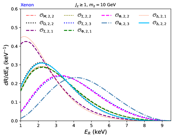
Figure 1: Expected differential scattering rate (1.5) normalized to 1 event for a 10 GeV mass WIMP with a xenon target and for the 10 irreducible effective operators ${\cal O}_{X,2,l}$ defined in Eqs. (3.22), assuming a WIMP of spin $j_{\chi}\geq$1.

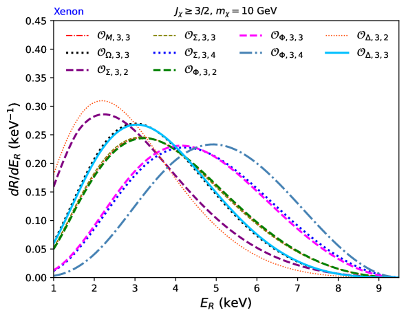
Figure 2: Same as Fig. 1 but for the 10 irreducible effective operators ${\cal O}_{X,3,l}$ and assuming a WIMP of spin $j_{\chi}\geq$3/2.

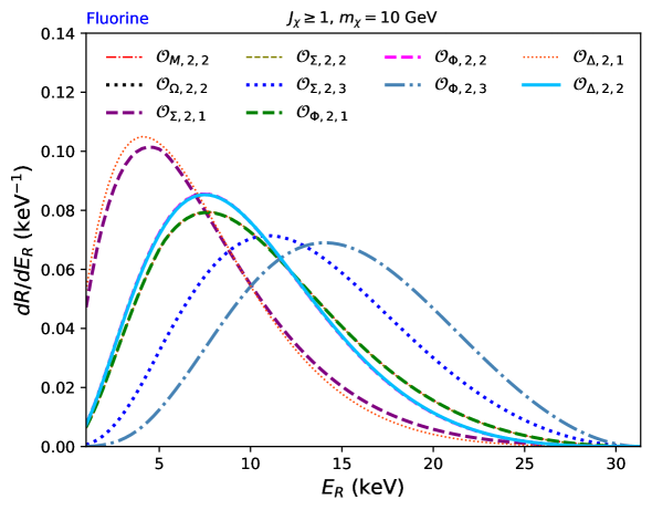
Figure 3: Same as Fig. 1 but for a fluorine target.

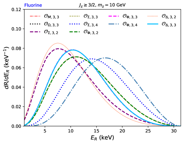
Figure 4: Same as in Fig. 2 but for a fluorine target.

7 Conclusions

In the present paper we have introduced a systematic approach that, in the one–nucleon approximation, describes the most general non-relativistic WIMP–nucleus interaction allowed by Galilean invariance for a WIMP of arbitrary spin. The resulting squared scattering amplitudes depend on the WIMP response functions of Eqs. (5.43), which are the main result of our paper, and on the same nuclear response functions as for WIMPs of spin $\leq$ 1. Many nuclear response functions are available in the literature for most of the targets used in WIMP direct detection experiments [26, 33].

In particular, we have expressed the WIMP–nucleon interaction Hamiltonian operators in terms of tensors irreducible under the rotation group. This has several advantages:

• it includes all the operators allowed by symmetry, including those that do not arise as the low–energy limit of standard point–like particle interactions with spin $\leq$1 mediators;

• it avoids double counting, allowing to show that some of the operators introduced in the literature for the spin-1 WIMP case are not independent (see Section 6.1);

• it greatly simplifies the calculation of the cross section, that was obtained from the two master equations (5.19-5.20) for the traces of WIMP spin operators;

• for a given WIMP spin $j_{\chi}$ the scattering cross section is given by a sum of cleanly separated contributions from irreducible operators of ranks 0, 1, 2, 3, …, up to $2j_{\chi}$, without interference terms (since irreducible operators of different rank do not interfere).

All the Wilson coefficients $c_{X,s,l}$ are defined up to arbitrary functions of the transferred momentum $q^{2}$. Moreover, as shown in Table 1, in some cases the change of basis from reducible to irreducible operators involves momentum–dependent coefficients.

From the phenomenological point of view, contributions from irreducible operators of higher rank are shifted to larger recoil energies compared with contributions from operators of lower rank. It may happen that lower rank operators vanish and the WIMP scattering rate is dominated by a higher rank operator. We expect this to lead to non–standard phenomenological consequences.

Appendix A Multipole expansion of a vector plane wave

It is well known that a plane wave $e^{i\vec{q}\cdot\vec{r}}$ can be expanded into spherical harmonics according to the equation

$$e^{i\vec{q}\cdot\vec{r}}=\sum_{L=0}^{\infty}\sum_{M=-L}^{L}4\pi i^{L}j_{L}(qr)Y_{LM}^{*}(\hat{q})Y_{LM}(\hat{r}).$$ (A.1)

Here $j_{L}(qr)$ is the spherical Bessel function of order $L$. Among equivalent forms of this expansion, Eq. (A.1) is a vector equation valid in any coordinate system that shows the explicit separate dependence on the unit vectors $\hat{q}$ and $\hat{r}$.

For a vector plane wave $\vec{\ell}\,e^{i\vec{q}\cdot\vec{r}}$, it is not hard to find in the literature expressions of its expansion into vector spherical harmonics in specific coordinate systems, for the most part with the $z$ axis chosen along the direction of the vector $\vec{q}$. Here we establish the following vector relation valid in all coordinate systems, showing the explicit separate dependence on the unit vectors $\hat{q}$ and $\hat{r}$ in analogy to Eq. (A.1).

$$e^{i\vec{q}\cdot\vec{r}}\,\vec{j}(\vec{r})=\sum_{J=0}^{\infty}\sum_{M=-J}^{J}4\pi i^{J}\bigg{[} -i\,\vec{Y}_{JM}^{({\rm L})*}(\hat{q})\,\,\bigg{(}\frac{1}{q}\frac{\partial M_{JM}(q,\vec{r})}{\partial\vec{r}}\bigg{)}\cdot\vec{j}(\vec{r})$$

$$+i\,\vec{Y}_{JM}^{({\rm TE})*}(\hat{q})\,\,\bigg{(}\!-\frac{i}{q}\frac{\partial}{\partial\vec{r}}\times\vec{M}^{M}_{JJ}(q,\vec{r})\bigg{)}\cdot\vec{j}(\vec{r})$$

$$+i\,\vec{Y}_{JM}^{({\rm TM})*}(\hat{q})\,\,\vec{M}^{M}_{JJ}(q,\vec{r})\cdot\vec{j}(\vec{r})\bigg{]}.$$ (A.2)

Here L, TE, and TM stand for longitudinal, transverse electric and transverse magnetic, respectively; the ${\rm TE}$ and ${\rm TM}$ terms start at $J=1$;

$$M_{JM}(q,\vec{r})=j_{J}(qr)Y_{JM}(\hat{r}),$$ (A.3)

$$\vec{M}^{M}_{JL}(q,\vec{r})=j_{J}(qr)\vec{Y}_{JLM}(\hat{r}).$$ (A.4)

Moreover,

$$\vec{Y}_{JM}^{({\rm L})}(\hat{q}) =\sqrt{\frac{J}{2J+1}}\vec{Y}_{J\,J-1\,M}(\hat{q})-\sqrt{\frac{J+1}{2J+1}}\vec{Y}_{J\,J+1\,M}(\hat{q})=\hat{q}\,Y_{JM}(\hat{q}),$$ (A.5)

$$\vec{Y}_{JM}^{({\rm TE})}(\hat{q}) =\sqrt{\frac{J+1}{2J+1}}\vec{Y}_{J\,J-1\,M}(\hat{q})+\sqrt{\frac{J}{2J+1}}\vec{Y}_{J\,J+1\,M}(\hat{q})=\frac{q}{\sqrt{J(J+1)}}\frac{\partial Y_{JM}(\hat{q})}{\partial\vec{q}},$$ (A.6)

$$\vec{Y}_{JM}^{({\rm TM})}(\hat{q}) =i\,\vec{Y}_{JJM}(\hat{q})=\hat{q}\times\vec{Y}_{JM}^{({\rm TE})}(\hat{q}),$$ (A.7)

are the longitudinal, transverse electric and transverse magnetic spherical harmonics, defined in terms of the vector spherical harmonics

$$\vec{Y}_{JLM}(\hat{q})=\sum_{\alpha=-L}^{L}\sum_{\beta=-1}^{1}C^{JM}_{L\alpha 1\beta}\,Y_{L\alpha}(\hat{q})\,\hat{e}_{\beta},$$ (A.8)

where $C^{JM}_{L\alpha 1\beta}$ is the Clebsch-Gordan coefficient for coupling angular momenta $L\alpha$ and $1\beta$ into $JM$, and $\hat{e}_{\beta}$ is the standard spherical basis

$$\hat{e}_{+1}=-(\hat{x}+i\hat{y})/\sqrt{2},\qquad\hat{e}_{0}=\hat{z},\qquad\hat{e}_{-1}=(\hat{x}-i\hat{y})/\sqrt{2}.$$ (A.9)

Eq. (A.2) can be obtained as follows. Write

$$\vec{\ell}\cdot\vec{j}\,e^{i\vec{q}\cdot\vec{r}}=\sum_{JM}\bigg{[}c^{({\rm L})}_{JM}\,\frac{1}{q}\frac{\partial M_{JM}(q,\vec{r})}{\partial\vec{r}}-ic^{({\rm TE})}_{JM}\,\frac{1}{q}\frac{\partial}{\partial\vec{r}}\times\vec{M}^{M}_{JJ}(q,\vec{r})+c^{({\rm TM})}_{JM}\,\vec{M}^{M}_{JJ}(q,\vec{r})\bigg{]}\cdot\vec{j}.$$ (A.10)

By using the relations

$$\frac{\partial M_{JM}(q,\vec{r})}{\partial\vec{r}}=q\bigg{(}\sqrt{\frac{J}{2J+1}}\vec{M}^{M}_{J\,J-1}+\sqrt{\frac{J+1}{2J+1}}\vec{M}^{M}_{J\,J+1}\bigg{)},$$ (A.11)

and

$$\frac{\partial}{\partial\vec{r}}\times\vec{M}^{M}_{JJ}(q,\vec{r})=iq\bigg{(}\sqrt{\frac{J+1}{2J+1}}\vec{M}^{M}_{J\,J-1}-\sqrt{\frac{J}{2J+1}}\vec{M}^{M}_{J\,J+1}\bigg{)},$$ (A.12)

express Eq. (A.10) in the form

$$\vec{\ell}\cdot\vec{j}\,e^{i\vec{q}\cdot\vec{r}}=\sum_{JLM}c_{JLM}\,j_{L}(qr)\,\vec{Y}_{JLM}(\hat{r})\cdot\vec{j},$$ (A.13)

where $L=J-1,J,J+1$ and

$$c^{({\rm L})}_{JM}=\sqrt{\frac{J}{2J+1}}c_{J\,J-1\,M}+\sqrt{\frac{J+1}{2J+1}}c_{J\,J+1\,M},$$ (A.14)

$$c^{({\rm TE})}_{JM}=\sqrt{\frac{J+1}{2J+1}}c_{J\,J-1\,M}+\sqrt{\frac{J}{2J+1}}c_{J\,J+1\,M},$$ (A.15)

$$c^{({\rm TM})}_{JM}=c_{JJM}.$$ (A.16)

The orthogonality relation for the vector spherical harmonics,

$$\int\vec{Y}^{*}_{JLM}(\hat{r})\cdot\vec{Y}_{J^{\prime}L^{\prime}M^{\prime}}(\hat{r})\,d\Omega_{r}=\delta_{JJ^{\prime}}\delta_{LL^{\prime}}\delta_{MM^{\prime}},$$ (A.17)

then gives

$$c_{JLM}=4\pi i^{L}\vec{\ell}\cdot\vec{Y}^{*}_{JLM}(\hat{q}).$$ (A.18)

Relations (A.5–A.7) finally lead to Eq. (A.2).

Appendix B Sum/average over nuclear spins

We provide here the details leading to Eq. (5.7). The matrix element of the effective WIMP–nucleon Hamiltonian between an initial nuclear state $|J_{i}M_{i}\rangle$ and a final nuclear state $\langle J_{f}M_{f}|$ can be expanded into multipoles using Eq. (5.5). Then the Wigner-Eckart theorem can be applied to the matrix element of each nuclear current multipole operator $\widehat{X}^{\tau}_{JM}(q)$ in the right-hand side of Eqs. (5.6),

$$\langle J_{f}M_{f}|\widehat{X}^{\tau}_{JM}(q)|J_{i}M_{i}\rangle=\frac{1}{\sqrt{2J_{f}+1}}\,\,C^{J_{f}M_{f}}_{J_{i}M_{i}JM}\,\,\langle J_{f}||\widehat{X}^{\tau}_{J}(q)||J_{i}\rangle,$$ (B.1)

where $C^{J_{f}M_{f}}_{J_{i}M_{i}JM}$ is the Clebsch-Gordan coefficient coupling angular momenta $J_{i}M_{i}$ and $JM$ into angular momentum $J_{f}M_{f}$, and $\langle J_{f}||\widehat{X}^{\tau}_{J}(q)||J_{i}\rangle$ is the reduced matrix element of the nuclear multipole operator. One then computes the sum/average over nuclear spins

$$\overline{H_{\rm f\,\!i}^{*}H_{\rm f\,\!i}}\equiv\frac{1}{2J_{i}+1}\sum_{M_{i}M_{f}}H_{\rm f\,\!i}^{*}H_{\rm f\,\!i}$$ (B.2)

using

$$\sum_{M_{i}M_{f}}C^{J_{f}M_{f}}_{J_{i}M_{i}JM}C^{J_{f}M_{f}}_{J_{i}M_{i}J^{\prime}M^{\prime}}=\frac{2J_{f}+1}{2J+1}\delta_{JJ^{\prime}}\delta_{MM^{\prime}}$$ (B.3)

and Eqs. (D.2)–(D.4). One obtains

$$\overline{H_{\rm f\,\!i}^{*}H_{\rm f\,\!i}}=\frac{4\pi}{2J_{i}+1}\sum_{J}\bigg{[} H_{J}^{*}H_{J}+\frac{1}{2}\big{(}\delta_{ij}-\hat{q}_{i}\hat{q}_{j}\big{)}\Big{(}H_{J,i}^{({\rm TE})*}H_{J,j}^{({\rm TE})}+H_{J,i}^{({\rm TM})*}H_{J,j}^{({\rm TM})}\Big{)}$$

$$-\hat{q}\cdot\mathop{\rm Re}\!\Big{(}\vec{H}_{J}^{({\rm TM})*}\times\vec{H}_{J}^{({\rm TE})}\Big{)}\bigg{]}.$$ (B.4)

Here

$$H_{J}=\sum_{\tau}\bigg{(}\widetilde{\ell}_{M}^{\tau}\,M_{J}^{\tau}-i\vec{\widetilde{\ell}}{}_{\Sigma}^{\tau}\cdot\hat{q}\,\Sigma_{J}^{\prime\prime\,\tau}-\frac{q}{m_{N}}\vec{\ell}_{\Delta}^{\tau}\cdot\hat{q}\,{\widetilde{\Delta}}_{J}^{\prime\prime\,\tau}-\frac{iq}{m_{N}}\vec{\ell}_{\Phi}^{\tau}\cdot\hat{q}\,\Phi_{J}^{\prime\prime\,\tau}-\frac{iq}{m_{N}}\ell_{\Omega}^{\tau}\,\Omega_{J}^{\tau}\bigg{)},$$ (B.5)

$$\vec{H}^{({\rm TE})}_{J}=\sum_{\tau}\bigg{(}-i\vec{\widetilde{\ell}}{}_{\Sigma}^{\tau}\,\Sigma_{J}^{\prime\,\tau}+\frac{q}{m_{N}}\vec{\ell}_{\Delta}^{\tau}\,\Delta_{J}^{\prime\,\tau}-\frac{iq}{m_{N}}\vec{\ell}_{\Phi}{\widetilde{\Phi}}_{J}^{\prime\,\tau}\bigg{)},$$ (B.6)

$$\vec{H}^{({\rm TM})}_{J}=\sum_{\tau}\bigg{(}i\vec{\widetilde{\ell}}{}_{\Sigma}^{\tau}\,\Sigma_{J}^{\tau}+\frac{q}{m_{N}}\vec{\ell}_{\Delta}^{\tau}\,\Delta_{J}^{\tau}+\frac{iq}{m_{N}}\vec{\ell}_{\Phi}\Phi_{J}^{\tau}\bigg{)},$$ (B.7)

with

$$X_{J}^{\tau}(q)=\langle J_{f}||\widehat{X}_{J}^{\tau}||J_{i}\rangle.$$ (B.8)

According to Table 7, the nuclear matrix elements that do not vanish in the nucleus ground state are

$$M^{\tau}_{J}(q),\Phi^{\prime\,\tau}_{J}(q),\Phi^{\prime\prime\,\tau}_{J}(q),\text{for $J$ even;}\qquad\Delta^{\tau}_{J}(q),\Sigma^{\prime\,\tau}_{J}(q),\Sigma^{\prime\prime\,\tau}_{J}(q),\text{for $J$ odd.}$$ (B.9)

This gives

$$H_{J} =\begin{cases}\widetilde{\ell}_{M}^{\tau}\,M_{J}^{\tau}-\frac{iq}{m_{N}}\vec{\ell}_{\Phi}^{\tau}\cdot\hat{q}\,\Phi_{J}^{\prime\prime\,\tau},&\text{for $J$ even,}\\[2.15277pt] -i\vec{\widetilde{\ell}}{}_{\Sigma}^{\tau}\cdot\hat{q}\,\Sigma_{J}^{\prime\prime\,\tau},&\text{for $J$ odd,}\end{cases}$$ (B.10)

$$\vec{H}_{JM}^{({\rm TE})} =\begin{cases}-\frac{iq}{m_{N}}\vec{\ell}_{\Phi}^{\tau}\,{\widetilde{\Phi}}_{J}^{\prime\,\tau},&\text{for $J$ even,}\\[2.15277pt] -i\vec{\widetilde{\ell}}{}_{\Sigma}^{\tau}\,\Sigma_{J}^{\prime\,\tau},&\text{for $J$ odd,}\end{cases}$$ (B.11)

$$\vec{H}_{JM}^{({\rm TM})} =\begin{cases}0,&\text{for $J$ even,}\\ \frac{q}{m_{N}}\vec{\ell}_{\Delta}^{\tau}\,\Delta_{J}^{\tau},&\text{for $J$ odd.}\end{cases}$$ (B.12)

Substituting the latter equations into Eq. (B.4) gives Eq. (5.7) in terms of the nuclear response functions defined in (5.8), with $F^{\tau\tau^{\prime}}_{XY}$ = $F^{\tau\tau^{\prime}}_{M}$, $F^{\tau\tau^{\prime}}_{\Sigma^{\prime}}$, $F^{\tau\tau^{\prime}}_{\Sigma^{\prime\prime}}$, $F^{\tau\tau^{\prime}}_{\Delta}$, $F^{\tau\tau^{\prime}}_{\Phi^{\prime\prime}}$, $F^{\tau\tau^{\prime}}_{\tilde{\Psi}^{\prime}}$, $F^{\tau\tau^{\prime}}_{M\Phi^{\prime\prime}}$ and $F^{\tau\tau^{\prime}}_{\Delta\Sigma^{\prime}}$.

Appendix C One-nucleon multipole operators

Here we list the one-nucleon multipole operators defined, for instance, in [39, 40, 41]. In the position-space representation, with $\vec{r}$ the position vector and $\vec{\sigma}$ the Pauli spin matrices, they are given by:

$$\widehat{M}_{JM}(q,\vec{r}) =j_{J}(qr)\,Y_{JM}(\hat{r}),$$

$$\widehat{\Delta}_{JM}(q,\vec{r}) =\vec{M}_{JJ}^{M}(q,\vec{r})\cdot\frac{1}{q}\frac{\partial}{\partial\vec{r}},$$

$$\widehat{\Delta}^{\prime}_{JM}(q,\vec{r}) =-i\bigg{(}\frac{1}{q}\frac{\partial}{\partial\vec{r}}\times\vec{M}_{JJ}^{M}(q,\vec{r})\bigg{)}\cdot\frac{1}{q}\frac{\partial}{\partial\vec{r}},$$

$$\widehat{\Delta}^{\prime\prime}_{JM}(q,\vec{r}) =\bigg{(}\frac{1}{q}\frac{\partial M_{JM}(q,\vec{r})}{\partial\vec{r}}\bigg{)}\cdot\frac{1}{q}\frac{\partial}{\partial\vec{r}},$$

$$\widehat{\Sigma}_{JM}(q,\vec{r}) =\vec{M}_{JJ}^{M}(q,\vec{r})\cdot\vec{\sigma},$$

$$\widehat{\Sigma}^{\prime}_{JM}(q,\vec{r}) =-i\bigg{(}\frac{1}{q}\frac{\partial}{\partial\vec{r}}\times\vec{M}_{JJ}^{M}(q,\vec{r})\bigg{)}\cdot\vec{\sigma},$$

$$\widehat{\Sigma}^{\prime\prime}_{JM}(q,\vec{r}) =\bigg{(}\frac{1}{q}\frac{\partial M_{JM}(q,\vec{r})}{\partial\vec{r}}\bigg{)}\cdot\vec{\sigma},$$

$$\widehat{\Phi}_{JM}(q,\vec{r}) =i\vec{M}_{JJ}^{M}(q,\vec{r})\cdot\bigg{(}\vec{\sigma}\times\frac{1}{q}\frac{\partial}{\partial\vec{r}}\bigg{)},$$

$$\widehat{\Phi}^{\prime}_{JM}(q,\vec{r}) =\bigg{(}\frac{1}{q}\frac{\partial}{\partial\vec{r}}\times\vec{M}_{JJ}^{M}(q,\vec{r})\bigg{)}\times\bigg{(}\vec{\sigma}\times\frac{1}{q}\frac{\partial}{\partial\vec{r}}\bigg{)},$$

$$\widehat{\Phi}^{\prime\prime}_{JM}(q,\vec{r}) =i\bigg{(}\frac{1}{q}\frac{\partial M_{JM}(q,\vec{r})}{\partial\vec{r}}\bigg{)}\cdot\bigg{(}\vec{\sigma}\times\frac{1}{q}\frac{\partial}{\partial\vec{r}}\bigg{)},$$

$$\widehat{\Omega}_{JM}(q,\vec{r}) =M_{JM}(q,\vec{r})\vec{\sigma}\cdot\frac{1}{q}\frac{\partial}{\partial\vec{r}}\,.$$ (C.1)

Moreover, the following definitions are given in [25] as implementation of Eq. (2.14),

$$\widehat{\widetilde{\Delta}}{}^{\prime\prime}_{JM}(q,\vec{r}) =\widehat{\Delta}^{\prime\prime}_{JM}(q,\vec{r})-\frac{1}{2}\widehat{M}_{JM}(q,\vec{r}),$$

$$\widehat{\widetilde{\Phi}}{}^{\prime}_{JM}(q,\vec{r}) =\widehat{\Phi}^{\prime}_{JM}(q,\vec{r})+\frac{1}{2}\widehat{\Sigma}_{JM}(q,\vec{r}),$$

$$\widehat{\widetilde{\Phi}}{}_{JM}(q,\vec{r}) =\widehat{\Phi}_{JM}(q,\vec{r})-\frac{1}{2}\widehat{\Sigma}^{\prime}_{JM}(q,\vec{r}),$$

$$\widehat{\widetilde{\Omega}}_{JM}(q,\vec{r}) =\widehat{\Omega}_{JM}(q,\vec{r})+\frac{1}{2}\widehat{\Sigma}^{\prime\prime}_{JM}(q,\vec{r})\,.$$ (C.2)

The one-nucleon operators appearing in Eqs. (5.2)–(5.4) are then

$$\widehat{X}_{JM}^{\tau}(q)=\sum_{N}\widehat{X}_{JM}(\vec{q},\vec{r}_{N})\,t^{\tau}_{N},$$ (C.3)

where $X=M,\Delta,\Delta^{\prime},\Delta^{\prime\prime},\Sigma,\Sigma^{\prime},\Sigma^{\prime\prime},\Phi,\Phi^{\prime},\Phi^{\prime\prime},\Omega,\widetilde{\Delta},\widetilde{\Phi},\widetilde{\Omega}$.

Appendix D Some mathematical identities

D.1 Sums of products of spherical harmonics over magnetic quantum number

In the sum/average over nuclear spins, one needs expressions for the sum over $M$ of products of scalar and vector spherical harmonics. The simplest one is for the case of the product of two scalar spherical harmonics. It is

$$\sum_{M=-J}^{J}Y_{JM}(\hat{r})\,Y^{*}_{JM}(\hat{r})=\frac{2J+1}{4\pi}.$$ (D.1)

Here we prove the following equations, written in dyadic notation (namely $\vec{a}\vec{b}\equiv a_{i}b_{j}$), with $\hat{r}$, $\hat{\uptheta}$, $\hat{\upphi}$ equal to the unit coordinate vectors in spherical coordinates $(r,\theta,\phi)$.

$$\sum_{M=-J}^{J}\vec{Y}^{({\rm TE})}_{JM}(\hat{r})\,Y^{*}_{JM}(\hat{r})=\sum_{M=-J}^{J}\vec{Y}^{({\rm TM})}_{JM}(\hat{r})\,Y^{*}_{JM}(\hat{r})=0,$$ (D.2)

$$\sum_{M=-J}^{J}\vec{Y}^{({\rm TE})}_{JM}(\hat{r})\,\vec{Y}^{({\rm TE})*}_{JM}(\hat{r})=\sum_{M=-J}^{J}\vec{Y}^{({\rm TM})}_{JM}(\hat{r})\,\vec{Y}^{({\rm TM})*}_{JM}(\hat{r})=\frac{2J+1}{4\pi}\,\frac{1}{2}\left(\hat{\uptheta}\,\hat{\uptheta}+\hat{\upphi}\,\hat{\upphi}\right),$$ (D.3)

$$\sum_{M=-J}^{J}\vec{Y}^{({\rm TM})}_{JM}(\hat{r})\,\vec{Y}^{({\rm TE})*}_{JM}(\hat{r})=\frac{2J+1}{4\pi}\,\frac{1}{2}\left(\hat{\upphi}\,\hat{\uptheta}-\hat{\uptheta}\,\hat{\upphi}\right).$$ (D.4)

To obtain Eqs. (D.2)–(D.4), one first writes

$$\vec{Y}^{({\rm L})}_{JM}(\hat{r}) =Y_{JM}(\hat{r})\,\hat{r},$$ (D.5)

$$\vec{Y}^{({\rm TE})}_{JM}(\hat{r}) =\frac{1}{\sqrt{J(J+1)}}\left[\frac{\partial Y_{JM}(\hat{r})}{\partial\theta}\,\hat{\uptheta}+\frac{1}{\sin\theta}\frac{\partial Y_{JM}(\hat{r})}{\partial\phi}\,\hat{\upphi}\right],$$ (D.6)

$$\vec{Y}^{({\rm TM})}_{JM}(\hat{r}) =\frac{1}{\sqrt{J(J+1)}}\left[-\frac{1}{\sin\theta}\frac{\partial Y_{JM}(\hat{r})}{\partial\phi}\,\hat{\uptheta}+\frac{\partial Y_{JM}(\hat{r})}{\partial\theta}\,\hat{\upphi}\right].$$ (D.7)

The sums over $M$ involving derivatives of the $Y_{JM}$ are evaluated by differentiating the addition theorem of spherical harmonics

$$\sum_{M=-J}^{J}Y_{JM}(\theta_{1},\phi_{1})\,Y^{*}_{JM}(\theta_{2},\phi_{2})=\frac{2J+1}{4\pi}\,P_{J}(\mu),$$ (D.8)

where $P_{J}(\mu)$ is the Legendre polynomial of order $J$ with

$$\mu=\cos\theta_{1}\cos\theta_{2}+\sin\theta_{1}\sin\theta_{2}\cos(\phi_{1}-\phi_{2}).$$ (D.9)

For example, with the $\to$ indicating the limit $(\theta_{1},\phi_{1})\to(\theta_{2},\phi_{2})$,

$$\sum_{M}\frac{\partial Y_{JM}(\theta_{1},\phi_{1})}{\partial\theta_{1}}\frac{\partial Y^{*}_{JM}(\theta_{2},\phi_{2})}{\partial\theta_{2}}=\frac{2J+1}{4\pi}\,\frac{\partial^{2}P_{J}(\mu)}{\partial\theta_{1}\partial\theta_{2}}\to\frac{2J+1}{4\pi}\,P^{\prime}_{J}(1).$$ (D.10)

In this way one finds, using $P^{\prime}_{J}(1)=J(J+1)/2$,

$$\sum_{M}\frac{\partial Y_{JM}}{\partial\theta}\frac{\partial Y^{*}_{JM}}{\partial\theta}=\sum_{M}\frac{1}{\sin^{2}\theta}\frac{\partial Y_{JM}}{\partial\phi}\frac{\partial Y^{*}_{JM}}{\partial\phi}=\frac{2J+1}{4\pi}\,\frac{J(J+1)}{2},$$ (D.11)

$$\sum_{M}\frac{\partial Y_{JM}}{\partial\theta}\frac{\partial Y^{*}_{JM}}{\partial\phi}=\sum_{M}\frac{\partial Y_{JM}}{\partial\theta}Y^{*}_{JM}=\sum_{M}\frac{\partial Y_{JM}}{\partial\phi}Y^{*}_{JM}=0.$$ (D.12)

Combining Eqs. (D.5)–(D.7) and (D.11)–(D.12) one obtains Eqs. (D.2)–(D.4).

D.2 Some relations between symmetric and symmetric traceless tensors

By definition, the symmetric traceless part $\overbracket{A_{i_{1}\cdot i_{s}}}{}$ of an rank-$s$ tensor $A_{i_{1}\cdots i_{s}}$ is obtained by first symmetrizing $A_{i_{1}\cdots i_{s}}$ completely with respect to all of its indices, and then subtracting all the possible traces, i.e., contractions of pairs of indices, double pairs of indices, …, $s/2$-tuple pairs of indices. There is a general formula for the resulting expression (cfr. Eq. (2.2) in [42] and [43], and (2.44) in [44], where the connection with Legendre polynomials is also explained),

$$\overbracket{A_{i_{1}\cdots i_{s}}}{}=\frac{1}{N_{s}}\sum_{p=0}^{\lfloor s/2\rfloor}C_{s,s-2p}\big{\{}\delta_{i_{1}i_{2}}\cdots\delta_{i_{2p-1}i_{2p}}S_{i_{2p+1}\cdots i_{s}k_{1}k_{1}\cdots k_{p}k_{p}}\big{\}},$$ (D.13)

where the sum is over the number $p$ of traces (or of Kronecker $\delta$’s) in the right hand side, $\lfloor s/2\rfloor$ is the largest integer smaller than or equal to $s/2$,

$$C_{s,s-2p}=(-1)^{p}\frac{(2s-2p)!}{2^{s}(s-p)!(s-2p)!}$$ (D.14)

is the coefficient of $x^{s-2p}$ in the Legendre polynomial $P_{s}(x)$ of order $s$ (in the standard normalization $P_{s}(1)=1$),

$$N_{s}=C_{s,s},$$ (D.15)

$$S_{i_{1}\cdots i_{s}}=\big{\{}A_{i_{1}\cdots i_{s}}\big{\}},$$ (D.16)

and curly brackets indicate complete symmetrization with respect to the free indices inside the brackets,

$$\big{\{}A_{i_{1}\cdots i_{s}}\big{\}}=\frac{1}{s!}\,\sum_{\pi}A_{i_{\pi(1)}\cdots i_{\pi(s)}},$$ (D.17)

with the sum over the permutations $\pi$ of $12\cdots s$.

For products of spin operators $\vec{S}$ and a vector $\vec{q}$, Eq. (D.13) gives

$$\overbracket{(\vec{q}\cdot\vec{S})^{n}}{}=\sum_{k=0}^{\lfloor n/2\rfloor}c_{n,k}\,q^{2k}\vec{S}^{\,2k}\,(\vec{q}\cdot\vec{S})^{n-2k},$$ (D.18)

where

$$c_{n,k}=(-1)^{k}\frac{(n!)^{2}(2n-2k)!}{k!(2n)!(n-2k)!(n-k)!}.$$ (D.19)

Recall that for a particle of spin $j_{\chi}$,

$$\vec{S}^{\,2}=j_{\chi}(j_{\chi}+1),\qquad\vec{S}^{\,2k}=[j_{\chi}(j_{\chi}+1)]^{k}.$$ (D.20)

The quantity $c_{n,k}$ is the coefficient of $x^{n-2k}$ in the monic Legendre polynomial $\overline{P}_{n}(x)$ of degree $n$ (in a monic polynomial, the coefficient of the term of highest degree is equal to 1),

$$\overline{P}_{n}(x)=\frac{(2n-1)!!}{n!}P_{n}(x)=\sum_{k=0}^{\lfloor n/2\rfloor}c_{n,k}x^{n-2k}.$$ (D.21)

The first few cases, relevant for WIMPs of spin up to 2, are

$$\overbracket{\vec{q}\cdot\vec{S}}{}=\vec{q}\cdot\vec{S},$$ (D.22)

$$\overbracket{(\vec{q}\cdot\vec{S})^{2}}{}=(\vec{q}\cdot\vec{S})^{2}-\frac{1}{3}q^{2}\vec{S}^{2},$$ (D.23)

$$\overbracket{(\vec{q}\cdot\vec{S})^{3}}{}=(\vec{q}\cdot\vec{S})^{3}-\frac{3}{5}q^{2}\vec{S}^{2}(\vec{q}\cdot\vec{S}),$$ (D.24)

$$\overbracket{(\vec{q}\cdot\vec{S})^{4}}{}=(\vec{q}\cdot\vec{S})^{4}-\frac{6}{7}q^{2}\vec{S}^{2}(\vec{q}\cdot\vec{S})^{2}+\frac{3}{35}q^{4}\vec{S}^{4}.$$ (D.25)

The coefficients can be compared to those appearing in the Legendre polynomials

$$P_{1}(x)=x,$$ (D.26)

$$P_{2}(x)=\frac{3}{2}\bigg{(}x^{2}-\frac{1}{3}\bigg{)},$$ (D.27)

$$P_{3}(x)=\frac{5}{2}\bigg{(}x^{3}-\frac{3}{5}x\bigg{)},$$ (D.28)

$$P_{4}(x)=\frac{35}{8}\bigg{(}x^{4}-\frac{6}{7}x^{2}+\frac{3}{35}\bigg{)}.$$ (D.29)

The reason for the equality of these coefficients is that Legendre polynomials are the expressions in polar angles of the symmetric traceless tensors that define electrostatic multipoles. The identities that connect these quantities are

$$\big{(}\vec{q}\cdot\vec{\nabla}\big{)}^{l}\frac{1}{r}=(-1)^{l}\frac{(2l-1)!!}{r^{2l+1}}(\vec{q}\cdot\vec{r})^{l}=\frac{(-1)^{l}}{l!}\frac{P_{l}(\cos\theta)}{r^{2l+1}},$$ (D.30)

$$(\vec{q}\cdot\vec{r})^{l}=\frac{l!}{(2l-1)!!}q^{l}r^{l}P_{l}(\cos\theta),$$ (D.31)

where $\theta$ is the angle between $\vec{q}$ and $\vec{r}$.

A formula for products of spin operators $\vec{S}$ involving two vectors $\vec{q}$ and $\vec{a}$ is

$$\overbracket{(\vec{a}\cdot\vec{S})\,(\vec{q}\cdot\vec{S})^{n-1}}{}=\sum_{k=0}^{\lfloor n/2\rfloor}c_{n,k}\,\bigg{\{} \frac{2k}{n-2k}\,q^{2k-2}\vec{S}^{\,2k}\,\vec{a}\cdot\vec{q}\,\,\big{[}(\vec{q}\cdot\vec{S})^{n-2k}\big{]_{\rm sym}}$$

$$+\frac{n-4k}{n-2k}\,q^{2k}\vec{S}^{\,2k}\,\,\big{[}(\vec{a}\cdot\vec{S})\,(\vec{q}\cdot\vec{S})^{n-2k-1}\big{]_{\rm sym}}\bigg{\}}.$$ (D.32)

It can be obtained by replacing one of the directional derivatives $\vec{q}\cdot\vec{\nabla}$ in Eq. (D.30) with $\vec{a}\cdot\vec{\nabla}$, leading to the polynomials

$$P_{l}(a,x)=P_{l}(x)+\frac{a-x}{l}\frac{dP_{l}(x)}{dx}.$$ (D.33)

The first few cases are

$$\overbracket{\vec{a}\cdot\vec{S}}{}=\vec{a}\cdot\vec{S},$$ (D.34)

$$\overbracket{(\vec{a}\cdot\vec{S})\,(\vec{q}\cdot\vec{S})}{}=\big{[}(\vec{a}\cdot\vec{S})\,(\vec{q}\cdot\vec{S})\big{]_{\rm sym}}-\frac{1}{3}\,\vec{a}\cdot\vec{q}\,\vec{S}^{2},$$ (D.35)

$$\overbracket{(\vec{a}\cdot\vec{S})\,(\vec{q}\cdot\vec{S})^{2}}{}=\big{[}(\vec{a}\cdot\vec{S})\,(\vec{q}\cdot\vec{S})^{2}\big{]_{\rm sym}}-\frac{2}{5}\,(\vec{a}\cdot\vec{q})\,\vec{S}^{2}\,(\vec{q}\cdot\vec{S})-\frac{1}{5}q^{2}\vec{S}^{\,2}(\vec{a}\cdot\vec{S}),$$ (D.36)

$$\overbracket{(\vec{a}\cdot\vec{S})\,(\vec{q}\cdot\vec{S})^{3}}{}=\big{[}(\vec{a}\cdot\vec{S})\,(\vec{q}\cdot\vec{S})^{3}\big{]_{\rm sym}}-\frac{3}{7}\,(\vec{a}\cdot\vec{q})\,\vec{S}^{2}\,(\vec{q}\cdot\vec{S})^{2}$$

$$\qquad\qquad\qquad\quad\,\,-\frac{3}{7}q^{2}\vec{S}^{2}\big{[}(\vec{a}\cdot\vec{S})\,(\vec{q}\cdot\vec{S})\big{]_{\rm sym}}+\frac{3}{35}\,(\vec{a}\cdot\vec{q})\,q^{2}\vec{S}^{4}.$$ (D.37)

Compare the coefficients to those in $P_{l}(a,x)$,

$$P_{1}(a,x)=a,$$ (D.38)

$$P_{2}(a,x)=\frac{3}{2}\bigg{(}ax-\frac{1}{3}\bigg{)},$$ (D.39)

$$P_{3}(a,x)=\frac{5}{2}\bigg{(}ax^{2}-\frac{2}{5}x-\frac{1}{5}a\bigg{)},$$ (D.40)

$$P_{4}(a,x)=\frac{35}{8}\bigg{(}ax^{3}-\frac{3}{7}x^{2}-\frac{3}{7}ax+\frac{3}{35}\bigg{)}.$$ (D.41)

For completeness, we recall that

$$\big{[}(\vec{a}\cdot\vec{S})\,(\vec{q}\cdot\vec{S})\big{]_{\rm sym}}=\frac{1}{2}\Big{[}(\vec{a}\cdot\vec{S})\,(\vec{q}\cdot\vec{S})+(\vec{q}\cdot\vec{S})\,(\vec{a}\cdot\vec{S})\Big{]},$$ (D.42)

$$\big{[}(\vec{a}\cdot\vec{S})\,(\vec{q}\cdot\vec{S})^{2}\big{]_{\rm sym}}=\frac{1}{3}\Big{[}(\vec{a}\cdot\vec{S})\,(\vec{q}\cdot\vec{S})^{2}+(\vec{q}\cdot\vec{S})\,(\vec{a}\cdot\vec{S})\,(\vec{q}\cdot\vec{S})+(\vec{q}\cdot\vec{S})^{2}\,(\vec{a}\cdot\vec{S})\Big{]},$$ (D.43)

$$\big{[}(\vec{a}\cdot\vec{S})\,(\vec{q}\cdot\vec{S})^{3}\big{]_{\rm sym}}=\frac{1}{4}\Big{[}(\vec{a}\cdot\vec{S})\,(\vec{q}\cdot\vec{S})^{3}+(\vec{q}\cdot\vec{S})\,(\vec{a}\cdot\vec{S})\,(\vec{q}\cdot\vec{S})^{2}$$

$$\qquad\qquad\qquad\qquad\quad\,\,\,+(\vec{q}\cdot\vec{S})^{2}\,(\vec{a}\cdot\vec{S})\,(\vec{q}\cdot\vec{S})+(\vec{q}\cdot\vec{S})^{3}\,(\vec{a}\cdot\vec{S})\Big{]},$$ (D.44)

and so on.

Inverse relations to Eqs. (D.18) and (D.32), giving the symmetric products of spin operators in terms of the symmetric traceless products, are

$$\big{[}(\vec{q}\cdot\vec{S})^{n}\big{]_{\rm sym}}=\sum_{k=0}^{\lfloor n/2\rfloor}d_{n,k}\,q^{2k}\vec{S}^{\,2k}\,\overbracket{(\vec{q}\cdot\vec{S})^{n-2k}}{},$$ (D.45)

and

$$\big{[}(\vec{a}\cdot\vec{S})\,(\vec{q}\cdot\vec{S})^{n-1}\big{]_{\rm sym}}=\sum_{k=0}^{\lfloor n/2\rfloor}d_{n,k}\,\bigg{[} \frac{2k}{n}\,q^{2k-2}\vec{S}^{\,2k}\,\vec{a}\cdot\vec{q}\,\,\overbracket{(\vec{q}\cdot\vec{S})^{n-2k}}{}$$

$$+\frac{n-2k}{n}\,q^{2k}\vec{S}^{\,2k}\,\,\overbracket{(\vec{a}\cdot\vec{S})\,(\vec{q}\cdot\vec{S})^{n-2k-1}}{}\bigg{]},$$ (D.46)

where

$$d_{n,k}=\frac{(2k-1)!!(2n-4k+1)!!}{(2n-2k+1)!!}{n\choose 2k}.$$ (D.47)

The quantities $d_{n,k}$ appear in the expansion of powers of $x$ in monic Legendre polynomials,

$$x^{n}=\sum_{k=0}^{\lfloor n/2\rfloor}d_{n,k}\overline{P}_{n-2k}(x).$$ (D.48)

The first few cases are

$$\big{[}\vec{q}\cdot\vec{S}\big{]_{\rm sym}}=\overbracket{\vec{q}\cdot\vec{S}}{},$$ (D.49)

$$\big{[}(\vec{q}\cdot\vec{S})^{2}\big{]_{\rm sym}}=\overbracket{(\vec{q}\cdot\vec{S})^{2}}{}+\frac{1}{3}q^{2}\vec{S}^{\,2},$$ (D.50)

$$\big{[}(\vec{q}\cdot\vec{S})^{3}\big{]_{\rm sym}}=\overbracket{(\vec{q}\cdot\vec{S})^{3}}{}+\frac{3}{5}q^{2}\vec{S}^{\,2}\overbracket{\vec{q}\cdot\vec{S}}{},$$ (D.51)

$$\big{[}(\vec{q}\cdot\vec{S})^{4}\big{]_{\rm sym}}=\overbracket{(\vec{q}\cdot\vec{S})^{4}}{}+\frac{6}{7}q^{2}\vec{S}^{\,2}\overbracket{(\vec{q}\cdot\vec{S})^{2}}{}+\frac{1}{5}q^{4}\vec{S}^{\,4},$$ (D.52)

$$\big{[}\vec{a}\cdot\vec{S}\big{]_{\rm sym}}=\overbracket{\vec{a}\cdot\vec{S}}{},$$ (D.53)

$$\big{[}(\vec{a}\cdot\vec{S})\,(\vec{q}\cdot\vec{S})\big{]_{\rm sym}}=\overbracket{(\vec{a}\cdot\vec{S})\,(\vec{q}\cdot\vec{S})}{}+\frac{1}{3}\,\vec{a}\cdot\vec{q}\,\vec{S}^{\,2},$$ (D.54)

$$\big{[}(\vec{a}\cdot\vec{S})\,(\vec{q}\cdot\vec{S})^{2}\big{]_{\rm sym}}=\overbracket{(\vec{a}\cdot\vec{S})\,(\vec{q}\cdot\vec{S})^{2}}{}+\frac{2}{5}\,\vec{a}\cdot\vec{q}\,\vec{S}^{\,2}\overbracket{\vec{q}\cdot\vec{S}}{}+\frac{1}{5}q^{2}\vec{S}^{\,2}\overbracket{\vec{a}\cdot\vec{S}}{},$$ (D.55)

$$\big{[}(\vec{a}\cdot\vec{S})\,(\vec{q}\cdot\vec{S})^{3}\big{]_{\rm sym}}=\overbracket{(\vec{a}\cdot\vec{S})\,(\vec{q}\cdot\vec{S})^{3}}{}+\frac{3}{7}\,\vec{a}\cdot\vec{q}\,\vec{S}^{\,2}\overbracket{(\vec{q}\cdot\vec{S})^{2}}{}$$

$$\qquad\qquad\qquad\qquad+\frac{3}{7}q^{2}\vec{S}^{\,2}\overbracket{(\vec{a}\cdot\vec{S})\,(\vec{q}\cdot\vec{S})^{2}}{}+\frac{1}{5}\,\vec{a}\cdot\vec{q}\,q^{2}\vec{S}^{\,2}.$$ (D.56)

D.3 Formulas for WIMP spin averages

To prove Eqs. (5.19)–(5.20), we make use of the formula [38],

$$\frac{1}{2j_{\chi}+1}\mathop{\rm tr}\Big{(}\overbracket{S_{i_{1}}S_{i_{2}}\cdots S_{i_{s}}}{}\overbracket{S_{j_{1}}S_{j_{2}}\cdots S_{j_{s^{\prime}}}}{}\Big{)}=\delta_{ss^{\prime}}\,\frac{s!}{(2s+1)!!}K_{0}K_{1}\cdots K_{s-1}\,\mathit{\Delta}^{(s)}_{i_{1}i_{2}\cdots i_{s},j_{1}j_{2}\cdots j_{s}},$$ (D.57)

Here the tensor $\mathit{\Delta}^{(s)}_{i_{1}i_{2}\cdots i_{s},j_{1}j_{2}\cdots j_{s}}$ projects the symmetric traceless part of a rank-$s$ tensor [38]. In other words, it is defined by

$$\overbracket{S_{i_{s}}\cdots S_{i_{s}}}{}=\mathit{\Delta}^{(s)}_{i_{1}i_{2}\cdots i_{s},i^{\prime}_{1}i^{\prime}_{2}\cdots i^{\prime}_{s}}S_{i_{s}^{\prime}}\cdots S_{i_{s}^{\prime}}.$$ (D.58)

Saturating all the free indices of Eq (D.57) with the product of momenta $\hat{q}_{j_{1}}\cdots\hat{q}_{j_{s}}$, $\hat{q}_{j_{1}}\cdots\hat{q}_{j_{s^{\prime}}}$ one gets

$$\frac{1}{2j_{\chi}+1}\mathop{\rm tr} \Big{(}\overbracket{S_{i_{1}}\cdots S_{i_{s}}}{}\hat{q}_{i_{1}}\cdots\hat{q}_{i_{s}}\overbracket{S_{j_{1}}\cdots S_{j_{s^{\prime}}}}{}\hat{q}_{j_{1}}\cdots\hat{q}_{j_{s^{\prime}}}\Big{)}=$$

$$\delta_{ss^{\prime}}\,\frac{s!}{(2s+1)!!}K_{0}K_{1}\cdots K_{s-1}\,\overbracket{\hat{q}_{i_{1}}\cdots\hat{q}_{i_{s}}}{}\,\overbracket{\hat{q}_{j_{1}}\cdots\hat{q}_{j_{s}}}{}.$$ (D.59)

Eq. (5.19) follows from the identity

$$\overbracket{\hat{q}_{i_{1}}\cdots\hat{q}_{i_{s}}}{}\,\overbracket{\hat{q}_{j_{1}}\cdots\hat{q}_{j_{s}}}{}=\frac{1}{N_{s}},$$ (D.60)

where

$$N_{s}=\frac{(2s-1)!!}{s!}$$ (D.61)

is the coefficient of $x^{s}$ in the Legendre polynomial $P_{s}(x)$ of order $s$ (in the standard normalization $P_{s}(1)=1$).

To prove Eq. (5.20), write

$$\frac{1}{2j_{\chi}+1}\mathop{\rm tr} \Big{(}\overbracket{S_{i_{1}}\cdots S_{i_{s}}}{}\hat{q}_{i_{1}}\cdots\hat{q}_{i_{s-1}}a_{i_{s}}\overbracket{S_{j_{1}}\cdots S_{j_{s^{\prime}}}}{}\hat{q}_{j_{1}}\cdots\hat{q}_{j_{s^{\prime}-1}}b_{j_{s^{\prime}}}\Big{)}=$$

$$\delta_{ss^{\prime}}\,\frac{s!}{(2s+1)!!}K_{0}K_{1}\cdots K_{s-1}\,\overbracket{\hat{q}_{i_{1}}\cdots\hat{q}_{i_{s-1}}a_{i_{s}}}{}\,\overbracket{\hat{q}_{j_{1}}\cdots\hat{q}_{j_{s-1}}b_{i_{s}}}{}.$$ (D.62)

In section D.4 we show that

$$\overbracket{\hat{q}_{i_{1}}\cdots\hat{q}_{i_{s-1}}a_{i_{s}}}{}\,\overbracket{\hat{q}_{i_{1}}\cdots\hat{q}_{i_{s-1}}b_{i_{s}}}{}=\frac{s+1}{2sN_{s}}\,(\vec{a}\cdot\vec{b})\qquad\text{for $\vec{a}\cdot\vec{q}=0$.}$$ (D.63)

Thus write

$$a_{i_{s}}=\hat{q}_{i_{s}}\,a^{||}+a{}^{\perp}_{i_{s}},$$ (D.64)

where

$$a^{||}=\hat{q}_{i}a_{i},\qquad a{}^{\perp}_{i}=(\delta_{ij}-\hat{q}_{i}\hat{q}_{j})\,a{}^{\perp}_{j},$$ (D.65)

and similarly for $b_{i_{s}}$. Then using Eqs. (D.60) and (D.63),

$$\overbracket{\hat{q}_{i_{1}}\cdots\hat{q}_{i_{s-1}}a_{i_{s}}}{}\,\overbracket{\hat{q}_{j_{1}}\cdots\hat{q}_{j_{s-1}}b_{i_{s}}}{}= \overbracket{\hat{q}_{i_{1}}\cdots\hat{q}_{i_{s-1}}\hat{q}_{i_{s}}}{}\,\overbracket{\hat{q}_{j_{1}}\cdots\hat{q}_{j_{s-1}}\hat{q}_{i_{s}}}{}\,a^{||}\,b^{||}$$

$$+\overbracket{\hat{q}_{i_{1}}\cdots\hat{q}_{i_{s-1}}\hat{q}^{\phantom{\perp}}_{i_{s}}}{}\,\overbracket{\hat{q}_{j_{1}}\cdots\hat{q}_{j_{s-1}}b{}^{\perp}_{i_{s}}}{}\,a^{||}$$

$$+\overbracket{\hat{q}_{i_{1}}\cdots\hat{q}_{i_{s-1}}a{}^{\,+}_{i_{s}}}{}\,\overbracket{\hat{q}_{j_{1}}\cdots\hat{q}_{j_{s-1}}\hat{q}^{\phantom{\perp}}_{i_{s}}}{}\,b^{||}$$

$$+\overbracket{\hat{q}_{i_{1}}\cdots\hat{q}_{i_{s-1}}a{}^{\perp}_{i_{s}}}{}\,\overbracket{\hat{q}_{j_{1}}\cdots\hat{q}_{j_{s-1}}b{}^{\perp}_{i_{s}}}{}$$ (D.66)

$$= \frac{1}{N_{s}}\,a^{||}\,b^{||}+\frac{s+1}{2sN_{s}}\,(\vec{a}{}^{\perp}\cdot\vec{b}{}^{\perp})$$ (D.67)

$$= \frac{1}{N_{s}}\Big{[}\,\hat{q}_{i}\hat{q}_{j}+\frac{s+1}{2s}(\delta_{ij}-\hat{q}_{i}\hat{q}_{j})\Big{]}a_{i}b_{j}$$ (D.68)

Then Eq. (5.20) follows from combining Eqs. (D.62) and (D.68).

D.4 Proof of Eq. (D.63)

We apply formula (D.13) to the product $\hat{q}_{i_{1}}\cdots\hat{q}_{i_{s-1}}a_{i_{s}}$. The symmetrization gives

$$S^{(a)}_{i_{1}\cdots i_{s}}\equiv\big{\{}\hat{q}_{i_{1}}\cdots\hat{q}_{i_{s-1}}a_{i_{s}}\big{\}}=\frac{1}{s!}\,\sum_{\pi}\hat{q}_{i_{\pi(1)}}\cdots\hat{q}_{i_{\pi(s-1)}}a_{i_{\pi(s)}}.$$ (D.69)

Separating the permutations involving $a_{i_{1}}$, $a_{i_{2}}$, …, $a_{i_{s}}$ leads to

$$S^{(a)}_{i_{1}\cdots i_{s}}=\frac{1}{s!}\Big{[} a_{i_{1}}\!\!\!\!\sum_{\begin{subarray}{c}\pi\\ \text{without }i_{1}\end{subarray}}\hat{q}_{i_{\pi(1)}}\cdots\hat{q}_{i_{\pi(s-1)}}+a_{i_{2}}\!\!\!\!\sum_{\begin{subarray}{c}\pi\\ \text{without }i_{2}\end{subarray}}\hat{q}_{i_{\pi(1)}}\cdots\hat{q}_{i_{\pi(s-1)}}+\cdots$$

$$+a_{i_{s}}\!\!\!\!\sum_{\begin{subarray}{c}\pi\\ \text{without }i_{s}\end{subarray}}\hat{q}_{i_{\pi(1)}}\cdots\hat{q}_{i_{\pi(s-1)}}\big{]}$$ (D.70)

$$=\frac{1}{s!}\Big{[} a_{i_{1}}\hat{q}_{i_{2}}\cdots\hat{q}_{i_{s-1}}(s-1)!+a_{i_{2}}\hat{q}_{i_{1}}\hat{q}_{i_{3}}\cdots\hat{q}_{i_{s-1}}(s-1)!+\cdots$$

$$+a_{i_{s}}\hat{q}_{i_{1}}\cdots\hat{q}_{i_{s-1}}(s-1)!\big{]}$$ (D.71)

$$=\frac{1}{s}\Big{[} a_{i_{1}}\hat{q}_{i_{2}}\cdots\hat{q}_{i_{s-1}}+\hat{q}_{i_{1}}a_{i_{2}}\hat{q}_{i_{3}}\cdots\hat{q}_{i_{s-1}}+\cdots+\hat{q}_{i_{1}}\cdots\hat{q}_{i_{s-1}}a_{i_{s}}\big{]}.$$ (D.72)

In subtracting the traces, the assumption $\vec{a}\cdot\vec{q}=0$ simplifies the expressions considerably, because all contractions involving one index from $a$ and the other from $\hat{q}$ vanish. Contraction of one pair of indices gives

$$S^{(a)}_{i_{1}\cdots i_{s-2}kk}= \frac{1}{s}\Big{[}a_{i_{1}}\hat{q}_{i_{2}}\cdots\hat{q}_{i_{s-2}}\hat{q}_{k}\hat{q}_{k}+\hat{q}_{i_{1}}a_{i_{2}}\hat{q}_{i_{3}}\cdots\hat{q}_{i_{s-2}}\hat{q}_{k}\hat{q}_{k}+\cdots+\hat{q}_{i_{1}}\cdots\hat{q}_{i_{s-3}}a_{i_{s-2}}\hat{q}_{k}\hat{q}_{k}+$$

$$\qquad\hat{q}_{i_{1}}\cdots\hat{q}_{i_{s-3}}a_{i_{s-1}}a_{k}\hat{q}_{k}+\hat{q}_{i_{1}}\cdots\hat{q}_{i_{s-3}}a_{i_{s-1}}\hat{q}_{k}a_{k}\Big{]}$$

$$= \frac{1}{s}\Big{[}a_{i_{1}}\hat{q}_{i_{2}}\cdots\hat{q}_{i_{s-2}}+\hat{q}_{i_{1}}a_{i_{2}}\hat{q}_{i_{3}}\cdots\hat{q}_{i_{s-2}}+\cdots+\hat{q}_{i_{1}}\cdots\hat{q}_{i_{s-3}}a_{i_{s-2}}\Big{]}$$

$$= \frac{s-2}{s}\,S^{(a)}_{i_{1}\cdots i_{s-2}}.$$ (D.73)

The contractions of double pairs, triple pairs, etc., follow by recursion as

$$S^{(a)}_{i_{1}\cdots i_{s-4}k_{1}k_{1}k_{2}k_{2}} =\frac{s-2}{s}\,\frac{s-4}{s-2}\,S^{(a)}_{i_{1}\cdots i_{s-4}}=\frac{s-4}{s}\,S^{(a)}_{i_{1}\cdots i_{s-2}},$$ (D.74)

and in general

$$S^{(a)}_{i_{1}\cdots i_{s-2p}k_{1}k_{1}\cdots k_{p}k_{p}}=\frac{s-2p}{s}\,S^{(a)}_{i_{1}\cdots i_{s-2p}}.$$ (D.75)

Inserting the latter expression into formula (D.13) leads to

$$\overbracket{\hat{q}_{i_{1}}\cdots\hat{q}_{i_{s-1}}a_{i_{s}}}{}=\frac{1}{N_{s}}\sum_{p=0}^{\lfloor s/2\rfloor}C_{s,s-2p}\big{\{}\delta_{i_{1}i_{2}}\cdots\delta_{i_{2p-1}i_{2p}}S^{(a)}_{i_{2p+1}\cdots i_{s}}\big{\}}\frac{s-2p}{s}.$$ (D.76)

We now consider the product $\overbracket{\hat{q}_{i_{1}}\cdots\hat{q}_{i_{s-1}}a_{i_{s}}}{}\,\overbracket{\hat{q}_{j_{1}}\cdots\hat{q}_{j_{s-1}}b_{i_{s}}}{}$, with $\vec{a}\cdot\vec{q}=0$. The symmetric traceless operation on the left forces a symmetric traceless operation on the right, so we can write

$$\overbracket{\hat{q}_{i_{1}}\cdots\hat{q}_{i_{s-1}}a_{i_{s}}}{}\,\overbracket{\hat{q}_{i_{1}}\cdots\hat{q}_{i_{s-1}}b_{i_{s}}}{}=\overbracket{\hat{q}_{i_{1}}\cdots\hat{q}_{i_{s-1}}a_{i_{s}}}{}\,\hat{q}_{i_{1}}\cdots\hat{q}_{i_{s-1}}b_{i_{s}}.$$ (D.77)

Inserting Eq. (D.76), and using

$$\delta_{i_{1}i_{2}}\cdots\delta_{i_{2p-1}i_{2p}}S_{i_{1}\cdots i_{s}}=S_{i_{2p+1}\cdots i_{s}k_{1}k_{1}\cdots k_{p}k_{p}}=\frac{s-2p}{s}S_{i_{2p+1}\cdots i_{s}},$$ (D.78)

we obtain

$$\overbracket{\hat{q}_{i_{1}}\cdots\hat{q}_{i_{s-1}}a_{i_{s}}}{}\,\overbracket{\hat{q}_{j_{1}}\cdots\hat{q}_{j_{s-1}}b_{i_{s}}}{}$$

$$\qquad=\sum_{p=0}^{\lfloor s/2\rfloor}\frac{C_{s,s-2p}}{N_{s}}\,\frac{s-2p}{s}\big{\{}\delta_{i_{1}i_{2}}\cdots\delta_{i_{2p-1}i_{2p}}S^{(a)}_{i_{2p+1}\cdots i_{s}}\big{\}}\hat{q}_{i_{1}}\cdots\hat{q}_{i_{s-1}}b_{i_{s}}$$

$$\qquad=\sum_{p=0}^{\lfloor s/2\rfloor}\frac{C_{s,s-2p}}{N_{s}}\,\frac{s-2p}{s}\big{\{}\delta_{i_{1}i_{2}}\cdots\delta_{i_{2p-1}i_{2p}}S^{(a)}_{i_{2p+1}\cdots i_{s}}\big{\}}\,\big{\{}\hat{q}_{i_{1}}\cdots\hat{q}_{i_{s-1}}b_{i_{s}}\big{\}}$$

$$\qquad=\sum_{p=0}^{\lfloor s/2\rfloor}\frac{C_{s,s-2p}}{N_{s}}\,\frac{s-2p}{s}\big{\{}\delta_{i_{1}i_{2}}\cdots\delta_{i_{2p-1}i_{2p}}S^{(a)}_{i_{2p+1}\cdots i_{s}}\big{\}}\,S^{(b)}_{i_{1}\cdots i_{s}}$$

$$\qquad=\sum_{p=0}^{\lfloor s/2\rfloor}\frac{C_{s,s-2p}}{N_{s}}\,\frac{s-2p}{s}\delta_{i_{1}i_{2}}\cdots\delta_{i_{2p-1}i_{2p}}S^{(a)}_{i_{2p+1}\cdots i_{s}}\,S^{(b)}_{i_{1}\cdots i_{s}}$$

$$\qquad=\sum_{p=0}^{\lfloor s/2\rfloor}\frac{C_{s,s-2p}}{N_{s}}\,\Big{(}\frac{s-2p}{s}\Big{)}^{2}S^{(a)}_{i_{2p+1}\cdots i_{s}}\,S^{(b)}_{i_{2p+1}\cdots i_{s}}$$ (D.79)

To find the product $S^{(a)}_{i_{1}\cdots i_{n}}S^{(b)}_{i_{1}\cdots i_{n}}$, we write

$$S_{i_{1}\cdots i_{n}}S_{i_{1}\cdots i_{n}}=\frac{1}{n^{2}} \Big{[}a_{i_{1}}\hat{q}_{i_{2}}\cdots\hat{q}_{i_{n}}+\hat{q}_{i_{1}}a_{i_{2}}\hat{q}_{i_{3}}\cdots\hat{q}_{i_{n}}+\cdots+\hat{q}_{i_{1}}\cdots\hat{q}_{i_{n-1}}a_{i_{n}}\Big{]}$$

$$\Big{[}b_{i_{1}}\hat{q}_{i_{2}}\cdots\hat{q}_{i_{n}}+\hat{q}_{i_{1}}b_{i_{2}}\hat{q}_{i_{3}}\cdots\hat{q}_{i_{n}}+\cdots+\hat{q}_{i_{1}}\cdots\hat{q}_{i_{n-1}}b_{i_{n}}\Big{]}.$$ (D.80)

Now all cross terms in the product of the two square brackets have $a_{i}q_{i}=0$ and so are zero. Only the square terms remain, and there are $n$ of them. Thus,

$$S_{i_{1}\cdots i_{n}}S_{i_{1}\cdots i_{n}}=\frac{1}{n}(\vec{a}\cdot\vec{b}).$$ (D.81)

Hence,

$$\overbracket{\hat{q}_{i_{1}}\cdots\hat{q}_{i_{s-1}}a_{i_{s}}}{}\,\overbracket{\hat{q}_{j_{1}}\cdots\hat{q}_{j_{s-1}}b_{i_{s}}}{} =\sum_{p=0}^{\lfloor s/2\rfloor}\frac{C_{s,s-2p}}{N_{s}}\,\Big{(}\frac{s-2p}{s}\Big{)}^{2}\frac{1}{s-2p}(\vec{a}\cdot\vec{b})$$

$$=(\vec{a}\cdot\vec{b})\frac{1}{s^{2}N_{s}}\sum_{p=0}^{\lfloor s/2\rfloor}(s-2p)\,C_{s,s-2p}.$$ (D.82)

To evaluate the last sum, we recall that by definition of $C_{s,s-2p}$,

$$P_{s}(x)=\sum_{p=0}^{\lfloor s/2\rfloor}C_{s,s-2p}\,x^{s-2p}.$$ (D.83)

Taking one derivative,

$$P^{\prime}_{s}(x)=\sum_{p=0}^{\lfloor s/2\rfloor}(s-2p)C_{s,s-2p}\,x^{s-2p}.$$ (D.84)

Thus

$$\sum_{p=0}^{\lfloor s/2\rfloor}(s-2p)\,C_{s,s-2p}=P^{\prime}_{s}(1)=\frac{s(s+1)}{2}.$$ (D.85)

We conclude that

$$\overbracket{\hat{q}_{i_{1}}\cdots\hat{q}_{i_{s-1}}a_{i_{s}}}{}\,\overbracket{\hat{q}_{j_{1}}\cdots\hat{q}_{j_{s-1}}b_{i_{s}}}{}=\frac{s+1}{2sN_{s}}(\vec{a}\cdot\vec{b}),$$ (D.86)

which is Eq. (D.63).

References

- [1] S. Chang, A. Pierce and N. Weiner, Momentum Dependent Dark Matter Scattering, JCAP 1001 (2010) 006, [0908.3192].
- [2] B. A. Dobrescu and I. Mocioiu, Spin-dependent macroscopic forces from new particle exchange, JHEP 11 (2006) 005, [hep-ph/0605342].
- [3] J. Fan, M. Reece and L.-T. Wang, Non-relativistic effective theory of dark matter direct detection, JCAP 1011 (2010) 042, [1008.1591].
- [4] J. Hisano, K. Ishiwata, N. Nagata and M. Yamanaka, Direct Detection of Vector Dark Matter, Prog. Theor. Phys. 126 (2011) 435–456, [1012.5455].
- [5] J. Hisano, K. Ishiwata, N. Nagata and T. Takesako, Direct Detection of Electroweak-Interacting Dark Matter, JHEP 07 (2011) 005, [1104.0228].
- [6] R. J. Hill and M. P. Solon, WIMP-nucleon scattering with heavy WIMP effective theory, Phys. Rev. Lett. 112 (2014) 211602, [1309.4092].
- [7] V. Gluscevic and A. H. G. Peter, Understanding WIMP-baryon interactions with direct detection: A Roadmap, JCAP 1409 (2014) 040, [1406.7008].
- [8] M. Cirelli, E. Del Nobile and P. Panci, Tools for model-independent bounds in direct dark matter searches, JCAP 1310 (2013) 019, [1307.5955].
- [9] S. Chang, R. Edezhath, J. Hutchinson and M. Luty, Effective WIMPs, Phys. Rev. D89 (2014) 015011, [1307.8120].
- [10] R. Catena, Prospects for direct detection of dark matter in an effective theory approach, JCAP 1407 (2014) 055, [1406.0524].
- [11] R. Catena, Dark matter directional detection in non-relativistic effective theories, JCAP 1507 (2015) 026, [1505.06441].
- [12] J. Hisano, K. Ishiwata and N. Nagata, QCD Effects on Direct Detection of Wino Dark Matter, JHEP 06 (2015) 097, [1504.00915].
- [13] R. Catena and P. Gondolo, Global fits of the dark matter-nucleon effective interactions, JCAP 1409 (2014) 045, [1405.2637].
- [14] SuperCDMS collaboration, K. Schneck et al., Dark matter effective field theory scattering in direct detection experiments, Phys. Rev. D91 (2015) 092004, [1503.03379].
- [15] R. Catena and P. Gondolo, Global limits and interference patterns in dark matter direct detection, JCAP 1508 (2015) 022, [1504.06554].
- [16] H. Rogers, D. G. Cerdeno, P. Cushman, F. Livet and V. Mandic, Multidimensional effective field theory analysis for direct detection of dark matter, Phys. Rev. D95 (2017) 082003, [1612.09038].
- [17] XENON collaboration, E. Aprile et al., Effective field theory search for high-energy nuclear recoils using the XENON100 dark matter detector, Phys. Rev. D96 (2017) 042004, [1705.02614].
- [18] CRESST collaboration, G. Angloher et al., Limits on Dark Matter Effective Field Theory Parameters with CRESST-II, Eur. Phys. J. C79 (2019) 43, [1809.03753].
- [19] R. J. Hill and M. P. Solon, Universal behavior in the scattering of heavy, weakly interacting dark matter on nuclear targets, Phys. Lett. B707 (2012) 539–545, [1111.0016].
- [20] R. J. Hill and M. P. Solon, Universal behavior in the scattering of heavy, weakly interacting dark matter on nuclear targets, Phys. Lett. B707 (2012) 539–545, [1111.0016].
- [21] M. Hoferichter, P. Klos and A. Schwenk, Chiral power counting of one- and two-body currents in direct detection of dark matter, Phys. Lett. B746 (2015) 410–416, [1503.04811].
- [22] M. Hoferichter, P. Klos, J. Menéndez and A. Schwenk, Analysis strategies for general spin-independent WIMP-nucleus scattering, Phys. Rev. D94 (2016) 063505, [1605.08043].
- [23] F. Bishara, J. Brod, B. Grinstein and J. Zupan, From quarks to nucleons in dark matter direct detection, JHEP 11 (2017) 059, [1707.06998].
- [24] M. W. Goodman and E. Witten, Detectability of Certain Dark Matter Candidates, Phys. Rev. D 31 (1985) 3059.
- [25] A. L. Fitzpatrick, W. Haxton, E. Katz, N. Lubbers and Y. Xu, The Effective Field Theory of Dark Matter Direct Detection, JCAP 1302 (2013) 004, [1203.3542].
- [26] N. Anand, A. L. Fitzpatrick and W. C. Haxton, Weakly interacting massive particle-nucleus elastic scattering response, Phys. Rev. C89 (2014) 065501, [1308.6288].
- [27] J. B. Dent, L. M. Krauss, J. L. Newstead and S. Sabharwal, General analysis of direct dark matter detection: From microphysics to observational signatures, Phys. Rev. D92 (2015) 063515, [1505.03117].
- [28] R. Catena, K. Fridell and M. B. Krauss, Non-relativistic Effective Interactions of Spin 1 Dark Matter, JHEP 08 (2019) 030, [1907.02910].
- [29] V. Barger, W.-Y. Keung and G. Shaughnessy, Spin dependence of dark matter scattering, Phys. Rev. 78 (Sep, 2008) 056007, [0806.1962].
- [30] G. Barello, S. Chang and C. A. Newby, A Model Independent Approach to Inelastic Dark Matter Scattering, Phys. Rev. D 90 (2014) 094027, [1409.0536].
- [31] Large-scale nuclear structure calculations for spin-dependent WIMP scattering with chiral effective field theory currents, Phys. Rev. D88 (2013) 083516, [1304.7684].
- [32] Nuclear structure aspects of spin-independent WIMP scattering off xenon, Phys. Rev. D91 (2015) 043520, [1412.6091].
- [33] R. Catena and B. Schwabe, Form factors for dark matter capture by the Sun in effective theories, JCAP 1504 (2015) 042, [1501.03729].
- [34] D. R. Yennie, M. M. Lévy and D. G. Ravenhall, Electromagnetic structure of nucleons, Rev. Mod. Phys. 29 (Jan, 1957) 144–157.
- [35] J. L. Friar, Relativistic Corrections to Electron Scattering by 2H, 3He, and 4He∗, Annals Phys. 81 (1973) 332–363.
- [36] J. J. Kelly, Nucleon charge and magnetization densities from Sachs form-factors, Phys. Rev. C 66 (2002) 065203, [hep-ph/0204239].
- [37] C. Perdrisat, V. Punjabi and M. Vanderhaeghen, Nucleon Electromagnetic Form Factors, Prog. Part. Nucl. Phys. 59 (2007) 694–764, [hep-ph/0612014].
- [38] S. Hess, Tensors for Physics. Springer, 2015.
- [39] J. De Forest, T. and J. Walecka, Electron scattering and nuclear structure, Adv. Phys. 15 (1966) 1–109.
- [40] T. W. Donnelly and J. D. Walecka, Electron Scattering and Nuclear Structure, Ann. Rev. Nucl. Part. Sci. 25 (1975) 329–405.
- [41] J. Walecka, Semileptonic weak interactions in nuclei, in Muon Physics (V. W. Hughes and C. Wu, eds.), pp. 113 – 218. Academic Press, 1975. DOI.
- [42] T. Damour and B. R. Iyer, Multipole analysis for electromagnetism and linearized gravity with irreducible cartesian tensors, Phys. Rev. D43 (1991) 3259–3272.
- [43] K. S. Thorne, Multipole Expansions of Gravitational Radiation, Rev. Mod. Phys. 52 (1980) 299–339.
- [44] F. A. E. Pirani, Introduction to Gravitational Radiation Theory, in Lectures on general relativity (A. Trautmann, F. A. E. Pirani and H. Bondi, eds.), pp. 249–374. Prentice Hall, Inc., Englewood Cliffs, NJ, 1965.