Mean-field spin-oscillation dynamics beyond the single-mode approximation for a harmonically trapped spin-1 Bose-Einstein condensate

Abstract

Compared to single-component Bose-Einstein condensates, spinor Bose-Einstein condensates display much richer dynamics. In addition to density oscillations, spinor Bose-Einstein condensates exhibit intriguing spin dynamics that is associated with population transfer between different hyperfine components. This work analyzes the validity of the widely employed single-mode approximation when describing the spin dynamics in response to a quench of the system Hamiltonian. The single-mode approximation assumes that the different hyperfine states all share the same time-independent spatial mode. This implies that the resulting spin Hamiltonian only depends on the spin interaction strength and not on the density interaction strength. Taking the spinor sodium Bose-Einstein condensate in the $f=1$ hyperfine manifold as an example and working within the mean-field theory framework, it is found numerically that the single-mode approximation misses, in some parameter regimes, intricate details of the spin and spatial dynamics. We develop a physical picture that explains the observed phenomenon. Moreover, using that the population oscillations described by the single-mode approximation enter into the effective potential felt by the mean-field spinor, we derive a semi-quantitative condition for when dynamical mean-field induced corrections to the single-mode approximation are relevant. Our mean-field results have implications for a variety of published and planned experimental studies.

I Introduction

Spinor Bose-Einstein condensates (BECs) display rich physics including spin domain formation, spin textures, topological excitations, and non-equilibrium quantum dynamics Kawaguchi and Ueda (2012); Stamper-Kurn and Ueda (2013). Spin-1 BECs are most commonly realized using sodium or rubidium atoms in the $f=1$ hyperfine manifold. Due to angular momentum conservation, the scattering of two $m=0$ atoms into the $m=\pm 1$ hyperfine states provides a path toward entanglement generation Kitagawa and Ueda (1993); Law et al. (1998); Duan et al. (2000); Pu and Meystre (2000); Riedel et al. (2010); Gross et al. (2010); Strobel et al. (2014); Lücke et al. (2011); Gross et al. (2011); Bookjans et al. (2011); Luo et al. (2017); Zou et al. (2018); here $m$ denotes the projection quantum number associated with the total angular momentum quantum number $f$ of a single atom. This route for entanglement generation, which can be viewed as an analogue of the four-wave mixing process in quantum optics, is behind a variety of proposals aimed at spin squeezing and metrological gain Vengalattore et al. (2007); Ma et al. (2011); Hamley et al. (2012a); Gabbrielli et al. (2015); Linnemann et al. (2016); Szigeti et al. (2017); Pezzè et al. (2018); Jie et al. (2019); Zhang and Schwettmann (2019).

In ²³Na and ⁸⁷Rb spin-1 BECs ($f=1$ manifold), the scattering length combination associated with the spin interactions is significantly smaller, in magnitude, than that associated with the density interactions; the ratio is approximately $28.1$ Knoop et al. (2011) and $215$ Stamper-Kurn and Ueda (2013) for sodium and rubidium, respectively. Correspondingly, the energy (time) scale for the spin interactions is smaller (larger) than for the density interactions. This observation is the key behind the single-mode approximation (SMA) Law et al. (1998); Pu et al. (1999); Yi et al. (2002); Zhang et al. (2003); Kawaguchi and Ueda (2012); Stamper-Kurn and Ueda (2013), which—in the context of a time-dependent situation—amounts to assuming that the shape, but not the amplitude, of the spatial density profile is frozen during the dynamics. As a consequence, the spatial modes enter into the spin Hamiltonian only in the form of the mean total density: a larger mean total density corresponds to a larger, in magnitude, spin-dependent interaction energy.

The SMA has been employed at the quantum level Law et al. (1998); Pu et al. (1999); Jie et al. (2019); Luo et al. (2017); Hamley et al. (2012b); Yang et al. (2019); Gerving et al. (2012) as well as at the mean-field level Zhang et al. (2005); Romano and de Passos (2004); Kronjäger et al. (2005, 2008); gerbier2019 . In the former, the spin Hamiltonian is treated fully quantum mechanically. In the latter, the mean value of the spin components is considered, resulting in a set of differential equations in terms of the fractional population of the $m=0$ mode and the relative phase that can be solved analytically. Intriguingly, the set of differential equations can be reproduced by defining a classical Hamiltonian in which the relative phase and fractional population play the role of the generalized coordinate and generalized momentum, respectively Zhang et al. (2005). This mapping allows one to visualize the dynamics using phase portraits in two-dimensional phase space.

The number of studies dedicated to assessing the validity of the mean-field SMA quantitatively in experimentally realistic dynamical settings is rather small Black et al. (2007); Liu et al. (2009); Zhao et al. (2014). This paper adds to this list and develops a simple framework for the emergence of dynamics beyond the SMA. Our work is related to Ref. Scherer et al. (2010), which observed quantum fluctuation-driven resonances experimentally and analyzed these resonances using the undepleted pump approximation, which assumes that the predominantly occupied spin component remains macroscopically occupied during the spin dynamics. Just as Ref. Scherer et al. (2010), we discuss a resonance effect. The characteristics that distinguish the resonances discussed in the present work from those discussed in Ref. Scherer et al. (2010) are: (i) In our work, the time-dependent SMA solutions create an effective time-dependent potential (driving term) for each $m$ channel. The effective potentials seen by the $m=\pm 1$ components in Ref. Scherer et al. (2010), in contrast, are time-independent. If the effective potential felt by one component supports an excited eigenstate whose energy is in resonance with the ground state energy of another channel, then coupling to an excited spatial mode becomes non-negligible. Physically, the above energy condition corresponds to a resonant scattering process in which two $m=0$ atoms get scattered into an $m=+1$ and an $m=-1$ atom. (ii) The coupling between the spin and spatial degrees discussed in this paper is mean-field driven and not, as in Ref. Scherer et al. (2010), quantum fluctuation driven.

Our solutions to the coupled mean-field Gross-Pitaevskii equations show that the coupling between the spin and spatial degrees of freedom develops dynamically, despite the fact that the initial state is well described within the mean-field SMA. The resonance condition, which depends on the interactions, can be avoided by tuning the single-particle detuning between the $m=0$ and $m=\pm 1$ atoms. Since the energy is conserved after the quench, the quench-induced dynamics discussed in our work is not accompanied by a relaxation to the ground state or the formation of (quasi-)static spin domains. Instead, spin structure develops and disappears as time proceeds. Our results are expected to be useful for the interpretation of past, ongoing, and future experiments.

The remainder of this article is structured as follows. Section II reviews the theoretical framework employed. Section III presents results for a ²³Na BEC under external axially symmetric harmonic confinement with fixed aspect ratio for various single-particle energy shifts $q$ and particle numbers $N$, using an initial state with vanishing magnetization ${\cal{M}}$. Beyond SMA physics is observed at the mean-field level. Section IV explains the observed beyond SMA effects. Finally, Sec. V summarizes our main results and provides an outlook.

II Theoretical framework

We consider a spin-1 BEC consisting of $N$ mass $M$ atoms in an external harmonic trap with angular frequencies $\omega_{x}$, $\omega_{y}$, and $\omega_{z}$. In addition to the harmonic confinement, the BEC atoms are exposed to external magnetic and microwave fields. The parameter $q$ in our equations below quantifies the strength of the energy shift that arises from the magnetic field induced quadratic Zeeman shift and the microwave field induced AC-Stark shift Gerbier et al. (2006); Zhao et al. (2014). The linear Zeeman shift energy does not appear explicitly in the equations since it can be eliminated by going to a rotating frame Zhang et al. (2003); Stamper-Kurn and Ueda (2013). Two different mean-field descriptions are considered:

• Approach A: A (2+2)-parameter mean-field SMA framework. This approach amounts to solving two sets of equations (one for the spatial and one for the spin degrees of freedom), both of which depend on two parameters.

• Approach B: A 5-parameter coupled Gross-Pitaevskii equations framework. This mean-field approach accounts for the coupling of the spatial and spin degrees of freedom.

In both approaches, the BEC is described by a three-component spinor $\vec{\Psi}(\vec{r},t)=(\Psi_{+1}(\vec{r},t),\Psi_{0}(\vec{r},t),\Psi_{-1}(\vec{r},t))^{T}$; however, the equations that govern $\Psi_{m}(\vec{r},t)$ differ for the two cases.

II.1 Approach A

The mean-field SMA Law et al. (1998); Pu et al. (1999); Yi et al. (2002); Zhang et al. (2003); Kawaguchi and Ueda (2012); Stamper-Kurn and Ueda (2013) assumes that the $m=+1$, $0$, and $-1$ components share the same spatial wave function $\psi_{\text{SMA}}(\vec{r})\exp(-\imath\epsilon t/\hbar)$, where the Gross-Pitaevskii orbital $\psi_{\text{SMA}}(\vec{r})$ and the chemical potential $\epsilon$ are solutions to the stationary single-component Gross-Pitaevskii equation

$$\bigg{[}H_{0}+g_{n}(N-1)|\psi_{\text{SMA}}(\vec{r})|^{2}\bigg{]}\psi_{\text{SMA}}(\vec{r})=\epsilon\psi_{\text{SMA}}(\vec{r})$$ (1)

with

$$H_{0}=\frac{-\hbar^{2}}{2M}\nabla_{\vec{r}}^{2}+V_{\text{trap}}(\vec{r})$$ (2)

and

$$V_{\text{trap}}(\vec{r})=\frac{1}{2}M\left(\omega_{x}^{2}x^{2}+\omega_{y}^{2}y^{2}+\omega_{z}^{2}z^{2}\right).$$ (3)

The Gross-Pitaevskii orbital $\psi_{\text{SMA}}(\vec{r})$ is assumed to be normalized to one and the density interaction strength $g_{n}$ is defined through Kawaguchi and Ueda (2012); Stamper-Kurn and Ueda (2013)

$$g_{n}=\frac{4\pi\hbar^{2}}{M}\frac{a_{0}+2a_{2}}{3},$$ (4)

where $a_{0}$ and $a_{2}$ are the $s$-wave scattering lengths for two colliding atoms with total spin angular momentum $F=0$ and $F=2$, respectively. Assuming axially symmetric harmonic confinement with $\omega_{\rho}=\omega_{x}=\omega_{y}$, $\psi_{\text{SMA}}(\vec{r})$ is governed by two dimensionless parameters, namely the dimensionless mean-field strength $g_{n}(N-1)/(a_{\text{ho},z}^{3}\hbar\omega_{z})$ [$a_{\text{ho},z}=\sqrt{\hbar/(M\omega_{z})}$] and the trap aspect ratio $\lambda$, $\lambda=\omega_{z}/\omega_{\rho}$.

The spinor components $\Psi_{m}(\vec{r},t)$ are then written as

$$\Psi_{m}(\vec{r},t)=\chi_{m}(t)\psi_{\text{SMA}}(\vec{r})\exp(-\imath\epsilon t/\hbar),$$ (5)

where the $\chi_{m}(t)$, which govern the spin dynamics, are given by $\chi_{m}(t)=\sqrt{\rho_{m}(t)}\exp\left[\imath\theta_{m}(t)\right]$. Here, $\theta_{m}(t)$ and $\rho_{m}(t)$ denote the phase and fractional population, normalized such that $\rho_{+1}(t)+\rho_{0}(t)+\rho_{-1}(t)=1$, of the $m$-th component. The SMA is argued to be applicable when the spin healing length $\xi_{s}$, $\xi_{s}=\hbar/\sqrt{2M|{c}_{s}|}$, is larger than the size of the BEC Stamper-Kurn and Ueda (2013); footnote_shl . Here, $c_{s}$ is the spin interaction energy, $c_{s}=g_{s}\overline{n}_{\text{SMA}}$, where the spin interaction strength $g_{s}$ Kawaguchi and Ueda (2012); Stamper-Kurn and Ueda (2013) is given by

$$g_{s}=\frac{4\pi\hbar^{2}}{M}\frac{a_{2}-a_{0}}{3}$$ (6)

and the mean density $\overline{n}_{\text{SMA}}$ by $\overline{n}_{\text{SMA}}=N\int|\psi_{\text{SMA}}(\vec{r})|^{4}d\vec{r}$. Looking ahead, we also define the density interaction energy $c_{n}$, $c_{n}=g_{n}{\overline{n}}_{\text{SMA}}$.

The equations that govern the fractional populations and phases can be conveniently written in terms of the magnetization ${\cal{M}}$, which is conserved throughout the time dynamics, and the relative phase $\theta(t)$ between the spinors, ${\cal{M}}=\rho_{+1}(t)-\rho_{-1}(t)$ and $\theta(t)=2\theta_{0}(t)-\theta_{+1}(t)-\theta_{-1}(t)$. With these definitions, the coupled equations of motion read Zhang et al. (2005)

$$\frac{\hbar}{2c_{s}}\frac{d\rho_{0}(t)}{dt}=-\rho_{0}(t)\sqrt{[1-\rho_{0}(t)]^{2}-{\cal{M}}^{2}}\sin(\theta(t))$$ (7)

and

$$-\frac{\hbar}{2c_{s}}\frac{d\theta(t)}{dt}=-\frac{q}{c_{s}}+1-2\rho_{0}(t)$$

$$+\frac{1-3\rho_{0}(t)+2[\rho_{0}(t)]^{2}-{\cal{M}}^{2}}{\sqrt{[1-\rho_{0}(t)]^{2}-{\cal{M}}^{2}}}\cos(\theta(t)).$$ (8)

Equations (7) and (II.1) show that the mean-field spin dynamics within the SMA is fully determined by two parameters, namely the “dimensionless energy” $q/c_{s}$ and the “dimensionless time” $t/(\hbar/c_{s})$. Since the static spatial mode and the spin dynamics are decoupled and each is governed by two parameters (throughout, we are considering axially symmetric harmonic confinement), we refer to the mean-field SMA as a (2+2)-parameter framework. It should be noted, however, that ${\overline{n}}_{\text{SMA}}$, which is determined by the static spatial mode, enters via the quantity $c_{s}$ into the equations that determine the spin dynamics.

As already alluded to in Sec. I, Eqs. (7) and (II.1) can be interpreted as Hamilton’s equations of motion of a classical Hamiltonian, with $\theta(t)$ and $\rho_{0}(t)$ playing the roles of the generalized coordinate and associated generalized momentum. Within this framework, the spin energy $E_{s}$ is conserved Zhang et al. (2005). Figures 1(a)-1(d) show the phase portrait for $q/c_{s}=1/2$, $1$, $3/2$, and $2$, respectively. Given $\rho_{0}(0)$ and $\theta(0)$, the dynamics proceeds along a fixed energy trajectory (lines in Fig. 1). Depending on the initial conditions, the trajectories correspond to periodic phase solutions (solid lines in Fig. 1) or running phase solutions (dashed lines in Fig. 1). For both classes of solutions, $\rho_{0}(t)$ is characterized by a fixed period and amplitude. Our calculations in Sec. III consider initial states with $\rho_{0}(0)=1/2$, $\rho_{+1}(0)=\rho_{-1}(0)=1/4$, and $\theta(0)=0$ (see blue dots in Fig. 1).

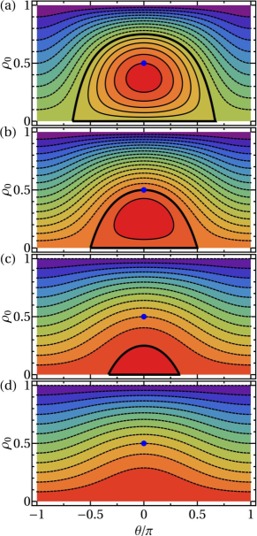
Figure 1: Phase portraits illustrating the mean-field SMA spin dynamics for ${\cal{M}}=0$ and (a) $q/c_{s}=1/2$, (b) $q/c_{s}=1$, (c) $q/c_{s}=3/2$, and (d) $q/c_{s}=2$. The lines show equally spaced trajectories with fixed $E_{s}/c_{s}$; the dimensionless energy spacing is $1/20$, $1/16$, $1/8$, and $1/6$ in panels (a)-(d), respectively. The blue dots mark the initial conditions considered in Sec. III; they correspond to $E_{s}/c_{s}=3/4$, $1$, $5/4$, and $3/2$ in panels (a)-(d), respectively. The separatrix that divides the periodic phase solutions (solid lines) and running phase solutions (dashed lines) is shown by a thick black line in panels (a)-(c); panel (d) supports only running phase and no periodic phase solutions.

II.2 Approach B

Even if the initial state is structureless and, e.g., well described by a Thomas-Fermi profile, spatial structure may develop during the time dynamics. Indeed, the formation of spatial structure during spin oscillation dynamics for spin-1 ²³Na and ⁸⁷Rb BECs has been reported by several experimental groups Chang et al. (2005); Scherer et al. (2010, 2013); Vinit et al. (2013). So far the theoretical modeling of this structure formation has been, to the best of our knowledge, restricted to approximate frameworks in the form of reduced dimensionality coupled mean-field Gross-Pitaevskii simulations Pu et al. (1999) or a stability analysis at the quantum level Scherer et al. (2010); klempt2010 . The following paragraphs outline the time-dependent coupled mean-field Gross-Pitaevskii equations framework, which allows for the coupling of the spin and spatial degrees of freedom and makes no a priori assumption about the spatial dynamics of the orbitals.

The time-dependent mean-field Gross-Pitaevskii equations for the spinor $\vec{\Psi}(\vec{r},t)$, which capture beyond single-mode physics, can be conveniently written in matrix form Kawaguchi and Ueda (2012); Yi et al. (2002); Zhang et al. (2003); Pu et al. (1999, 2000)

$$\imath\hbar\frac{\partial\vec{\Psi}(\vec{r},t)}{\partial t}=\left[{\cal{L}}+\underline{E}_{\text{shift}}+\underline{V}_{\text{c}}(\vec{r},t)\right]\vec{\Psi}(\vec{r},t),$$ (9)

where

$${\cal{L}}=H_{0}+g_{n}(N-1)\sum_{m=0,\pm 1}|\Psi_{m}(\vec{r},t)|^{2};$$ (10)

${\underline{E}}_{\text{shift}}$ is a diagonal matrix with diagonal elements $q$, $0$, and $q$; and

$$\underline{V}_{\text{c}}(\vec{r},t)=g_{s}(N-1)\times$$

$$\left(\begin{array}[]{ccc}\sum_{m=\pm 1,0}|\Psi_{m}(\vec{r},t)|^{2}-2|\Psi_{-1}(\vec{r},t)|^{2}&\Psi_{0}(\vec{r},t)\left[\Psi_{-1}(\vec{r},t)\right]^{*}&0\\ \left[\Psi_{0}(\vec{r},t)\right]^{*}\Psi_{-1}(\vec{r},t)&\sum_{m=\pm 1,0}|\Psi_{m}(\vec{r},t)|^{2}-|\Psi_{0}(\vec{r},t)|^{2}&\left[\Psi_{0}(\vec{r},t)\right]^{*}\Psi_{+1}(\vec{r},t)\\ 0&\Psi_{0}(\vec{r},t)\left[\Psi_{+1}(\vec{r},t)\right]^{*}&\sum_{m=\pm 1,0}|\Psi_{m}(\vec{r},t)|^{2}-2|\Psi_{+1}(\vec{r},t)|^{2}\end{array}\right).$$ (14)

If the spin interactions vanish (i.e., if $g_{s}=0$), then the solutions are independent of the coupling matrix $\underline{V}_{\text{c}}(\vec{r},t)$ [see Eqs. (9) and (II.2)]. The pattern formation discussed in Sec. III crucially depends on the kinetic energy contributions in Eq. (9) [see also Eq. (10)], i.e., treatment of the coupled mean-field Gross-Pitaevskii equations within the Thomas-Fermi approximation yields qualitatively different results than treatment of the full coupled mean-field equations.

As discussed earlier, the spatial dynamics and the spin dynamics within the mean-field SMA depend each on two dimensionless parameters, namely, $g_{n}(N-1)/(a_{\text{ho},z}^{3}\hbar\omega_{z})$ and $\lambda$ for the spatial degrees and $q/c_{s}$ and $t/(\hbar/c_{s})$ for the spin degrees. The coupled Gross-Pitaevskii equations [see Eqs. (9)-(10)], in contrast, depend on five dimensionless parameters: $g_{n}(N-1)/(a_{\text{ho},z}^{3}\hbar\omega_{z})$, $\lambda$, $q/c_{s}$, $t/(\hbar/c_{s})$, and $g_{n}/g_{s}$. The ratio $g_{n}/g_{s}$ “connects” the spatial and spin degrees of freedom. The energy scales $\hbar\omega_{\rho}$, $\hbar\omega_{z}$, and $g_{n}(N-1)/a_{\text{ho},z}^{3}$ are—for typical experimental parameters—significantly larger than the energy scale $c_{s}$. This suggests that the dynamics that is resulting from these energy scales is faster than the “low-energy” spin population dynamics. In fact, the mean-field SMA assumes that the dynamics introduced by these high-energy scales is so fast that it can be safely averaged out. However, the coupling between the low- and high-energy degrees of freedom can, at least in principle, lead to an energy transfer between the associated degrees of freedom. While direct comparisons between Gross-Pitaevskii simulation results and experimental data were not made, Ref. Chang et al. (2005) attributed the experimentally observed damping of the spin oscillations for ⁸⁷Rb (positive $q$) to this energy transfer and, associated with it, the breakdown of the mean-field SMA.

III Numerical Results

We consider a spin-1 ²³Na condensate with $a_{0}=48.91a_{B}$ and $a_{2}=54.54a_{B}$ Knoop et al. (2011), where $a_{B}$ denotes the Bohr radius. To prepare the initial state, we imagine the following procedure. First, all atoms are loaded into the $m=-1$ state of the $f=1$ hyperfine manifold in the presence of a small magnetic field. Second, a radio-frequency pulse is applied to prepare a state with population fractions of $1/4$ and $1/2$ in the $m=\pm 1$ and $m=0$ hyperfine states of the $f=1$ manifold Zhao et al. (2014); Black et al. (2007).

The lines in Fig. 2 show the fractional population $\rho_{0}(t)$ as a function of time, obtained by solving the coupled Gross-Pitaevskii equations for $N=40000$ and an axially symmetric harmonic confinement with moderate aspect ratio of $\lambda=15/7\approx 2.143$ for four different $q$ values. For comparison, the mean-field SMA results are shown by open circles. For the smallest and largest $q/c_{s}$ considered [Figs. 2(a) and 2(d) are for $q/c_{s}=1/2$ and $2$, respectively], the mean-field SMA describes the full mean-field spin oscillation dynamics fairly accurately.

For $q/c_{s}=1$, in contrast, the results for the coupled Gross-Pitaevskii equations (Approach B) display spin oscillations with notably smaller period than the results for the mean-field SMA (Approach A) [$73$ ms versus $231$ ms, see the inset of Fig. 2(b)]. For this parameter combination, the coupling between the spin and spatial degrees of freedom speeds the spin oscillation dynamics up significantly, i.e., the mean-field Gross-Pitaevskii equations framework predicts a smaller period than the mean-field SMA framework. In the classical phase portrait, the initial state for $q/c_{s}=1$ is located on the separatrix. As can be seen from Fig. 1(b), this implies that the fractional population $\rho_{0}(t)$ is equal to zero half-way through the first oscillation of the fractional populations. The coupled Gross-Pitaevskii equations, in contrast, result in a small non-zero $\rho_{0}(t)$ half-way through the first oscillation of the fractional populations; specifically, the value of $\rho_{0}(t)$ for $t=36.4$ ms is approximately $0.019$, corresponding to about $700$ atoms in the $m=0$ hyperfine state. For such a low-atom BEC component, quantum fluctuations of the spin and/or spatial degrees of freedom may play a non-negligible role, suggesting that the applicability of the coupled Gross-Pitaevskii equations needs to be assessed carefully.

For $q/c_{s}=3/2$ [see Fig. 2(c)], the coupled Gross-Pitaevskii equations and the mean-field SMA both display spin population oscillations of—roughly—the same period. Intriguingly, however, the coupling between the spin and spatial degrees of freedom that is accounted for by the coupled Gross-Pitaevskii equations leads to a damping as well as an overall upward drift of the spin oscillation amplitude during the first few cycles. This upward drift is not captured by the mean-field SMA, which predicts fractional population oscillations with constant amplitude and period.

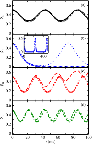
Figure 2: Comparison of the time-dependent fractional population $\rho_{0}(t)$ obtained using the coupled mean-field Gross-Pitaevskii equations (lines; Approach B) and mean-field SMA (open circles; Approach A). The coupled Gross-Pitaevskii equations simulations are performed for a sodium spin-1 BEC with $N=40000$ under external harmonic confinement characterized by $\omega_{\rho}=2\pi\times 70$ Hz and $\omega_{z}=2\pi\times 150$ Hz and interaction energies $c_{s}/h\approx 12.5$ Hz and $c_{n}/h\approx 350$ Hz. The single-particle energy scale $q$ is (a) $q/c_{s}=1/2$, (b) $q/c_{s}=1$, (c) $q/c_{s}=3/2$, and (d) $q/c_{s}=2$; this corresponds to $q/h\approx 6.23$ Hz, $12.5$ Hz, $18.7$ Hz, and $24.9$ Hz, respectively. The inset in panel (b) shows the mean-field SMA result for larger $t$.

Figure 3 shows selected integrated density profiles for the same parameters as those used in Fig. 2(c), i.e., for the case where the fractional population $\rho_{0}(t)$ drifts upward with time. Recall, this happens for $q/c_{s}=3/2$ and an initial state that is far away from the separatrix [see Fig. 1(c)]. The first two rows of Fig. 3 are for $t=38$ ms (after a bit more than one spin population oscillation) and the last two rows for $t=50$ ms (after about one and a half spin population oscillations). For both times, we see that the total integrated densities [see Figs. 3(ci) and 3(cii)] are close to what would be expected within the SMA and that the integrated densities for the spinor components [see Figs. 3(ai), 3(bi), 3(aii), and 3(bii)] display non-trivial structure, i.e., have much less resemblance with a Thomas-Fermi profile. Figure 3 shows that the structures of $n_{0}(x,y,t)$ for $t=38$ ms and of $n_{\pm 1}(x,y,t)$ for $t=50$ ms are quite similar. This observation is more general: We find that the “deformations” of the subcomponent densities $n_{0}(\vec{r},t)$ and $n_{\pm 1}(\vec{r},t)$, which combine to a Thomas-Fermi like total density $n(\vec{r},t)$, oscillate “out of phase”. This oscillatory structure in the subcomponent densities can clearly not be described within the SMA. We also solved the coupled mean-field Gross-Pitaevskii equations within the Thomas-Fermi approximation, which neglects the kinetic energy terms. This approximation yields qualitatively different densities than those displayed in Fig. 3. This shows that the observed structure formation depends sensitively on the interplay between the various energy terms in the coupled mean-field Gross-Pitaevskii equations.

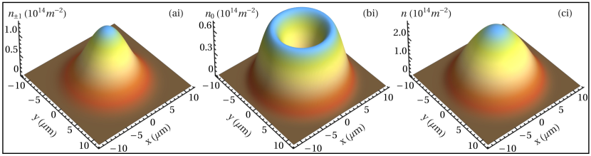
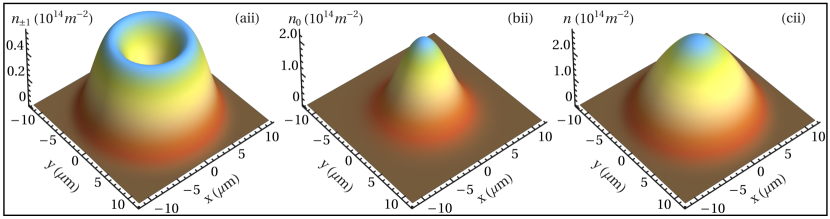
Figure 3: Snapshots of the integrated spatial density for a ²³Na spin-1 BEC with $N=40000$ under external harmonic confinement with $\omega_{\rho}=2\pi\times 70$ Hz and $\omega_{z}=2\pi\times 150$ Hz. The parameters are the same as those in Fig. 2(c), i.e., $q/c_{s}=3/2$, $c_{s}/h\approx 12.5$ Hz, and $c_{n}/h\approx 350$ Hz. The top row [panels (ai)-(ci)] and bottom row [panels (aii)-(cii)] are for $t=38$ ms and $50$ ms, respectively. The first, second, and third columns show the integrated densities $n_{\pm 1}(x,y,t)=N\int_{-\infty}^{\infty}|\Psi_{\pm 1}(\vec{r},t)|^{2}dz$, $n_{0}(x,y,t)=N\int_{-\infty}^{\infty}|\Psi_{0}(\vec{r},t)|^{2}dz$, and $n(x,y,t)=N\sum_{m=0,\pm 1}\int_{-\infty}^{\infty}|\Psi_{m}(\vec{r},t)|^{2}dz$, respectively.

The break-down of the SMA can be illustrated in a complementary approach, which relies on the fact that the mean-field SMA framework is fully governed by two dimensionless parameters, namely $q/c_{s}$ and $t/(\hbar/c_{s})$. The open circles in Fig. 4 show the fractional population $\rho_{0}(t)$, obtained within the mean-field SMA, as a function of the dimensionless time for $q/c_{s}=3/2$ [same data as in Fig. 2(c)]. For comparison, the red dashed, black solid, and blue dotted curves show the coupled mean-field Gross-Pitaevskii equations results for $N=40000$ [same data as in Fig. 2(c)], $N=10000$, and $N=80000$, respectively. In all cases, the trap frequencies $\omega_{\rho}$ and $\omega_{z}$ and coupling strengths $g_{s}$ and $g_{n}$ are the same as before. However, the value of $q$ is adjusted such that $q/c_{s}=3/2$ for all three $N$ values considered. Figure 4 shows that the $N=10000$ results are essentially on top of the SMA results, that the $N=80000$ oscillations have a slightly reduced oscillation period and amplitude, and that the $N=40000$ data display—as discussed in detail above—notable deviations from the SMA result. The ratio $\xi_{s}/R_{\text{TF},z}$ is $\approx 1.51$, $\approx 0.84$, and $\approx 0.63$ for $N=10000$, $40000$, and $80000$, respectively. Thus, the reliability of the mean-field SMA is not solely governed by the ratio between the spin healing length and the Thomas-Fermi radii.

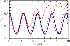
Figure 4: Fractional population $\rho_{0}(t)$, determined by the coupled Gross-Pitaevskii equations for a sodium spin-1 BEC under external harmonic confinement characterized by $\omega_{\rho}=2\pi\times 70$ Hz and $\omega_{z}=2\pi\times 150$ Hz. The black solid, red dashed, and blue dotted lines are for $N=10000$, $40000$, and $80000$, respectively. The $q$ value is adjusted for each $N$ such that $q/c_{s}=3/2$ for all three $N$ considered. For comparison, the open circles show the result from the calculations within the mean-field SMA; since the time is plotted in dimensionless units, the mean-field SMA result is independent of $N$. The open circles are essentially indistinguishable from the coupled Gross-Pitaevskii equations results for $N=10000$.

Focusing on initial states with fractional populations of $1/4$, $1/2$, and $1/4$ for the $m=+1$, $m=0$, and $m=-1$ hyperfine levels and vanishing relative phase, Figs. 2-4 identify two regimes where the mean-field SMA (Approach A) and coupled mean-field Gross-Pitaevskii equations (Approach B) yield different results. (i) Unlike Approach A, Approach B reveals an overall drift of the oscillating fractional population $\rho_{0}(t)$, which is accompanied by time-dependent non-Thomas-Fermi like pattern formation. (ii) The time periods of the spin oscillations predicted by Approach A and Approach B deviate significantly for $q/c_{s}\approx 1$, i.e., in the regime where the initial state is located on the separatrix. The next section develops a theory understanding of regime (i).

IV Physical picture

The effective potential picture developed in this section based on the time-dependent Gross-Pitaevskii equations [Eqs. (9)-(II.2)] is conceptually similar to the effective potential picture developed in Ref. Scherer et al. (2010), using a framework that accounts for quantum fluctuations. In that work, the $m=\pm 1$ modes are initially empty and the effective potentials are time independent. In our work, in contrast, the $m=\pm 1$ modes are initially macroscopically occupied and the effective potentials are time dependent.

In the absence of interactions and positive $q$, two colliding $m=0$ atoms must have an “extra” energy of $2q$ to scatter into an $m=+1$ atom and an $m=-1$ atom. If $q$ is negative, then an $m=+1$ atom and an $m=-1$ atom must have an “extra” energy of $2q$ to scatter into two $m=0$ atoms. To streamline the discussion, we assume in the remainder of this section that $q$ is positive; the arguments can be readily extended to the negative $q$ case. Since the $m=0$ channel needs—in the absence of interactions—an “extra” energy of $2q$ to be in resonance with the $m=\pm 1$ channels, we anticipate that—in the presence of interactions—the drifting occurs when there exists an excited state in the $m=0$ channel that is in resonance with the ground states of the $m=\pm 1$ channels. In this resonant regime, population transfer to the excited state can occur, leading to a density deformation (physics beyond the SMA). Since the different $m$ channels are coupled in the presence of interactions, the “excited” and “ground” states just referred to are associated with effective potentials that neglect the coupling between channels.

Our semi-quantitative estimate starts with Eqs. (9)-(II.2). We work within the SMA to evaluate the effective potential $\underline{V}_{\text{eff}}(\vec{r},t)$,

$$\underline{V}_{\text{eff}}(\vec{r},t)=V_{\text{trap}}(\vec{r})\underline{I}+\underline{E}_{\text{shift}}+\underline{V}_{\text{nl}}(\vec{r},t),$$ (15)

where

$$\underline{V}_{\text{nl}}(\vec{r},t)=\underline{V}_{c}(\vec{r},t)+g_{n}(N-1)\sum_{m}|\Psi_{m}(\vec{r},t)|^{2}\underline{I},$$ (16)

and $\underline{I}$ denotes the $3\times 3$ identity matrix. Specializing to the case where $|\Psi_{+1}(\vec{r},t)|=|\Psi_{-1}(\vec{r},t)|$, we find

$$\underline{V}_{\text{nl}}(\vec{r},t)=(N-1)|\psi_{\text{SMA}}(\vec{r})|^{2}\underline{V}_{\text{drive}}(t),$$ (17)

where

$$\underline{V}_{\text{drive}}(t)=g_{n}\underline{I}+g_{s}\underline{V}_{\text{diag}}(t)+g_{s}\underline{V}_{\text{off-diag}}(t).$$ (18)

Here, $\underline{V}_{\text{diag}}(t)$ is a diagonal matrix with elements $\rho_{0}(t)$, $1-\rho_{0}(t)$, and $\rho_{0}(t)$;

$$\underline{V}_{\text{off-diag}}(t)=\left(\begin{array}[]{ccc}0&d_{-1}(t)&0\\ d_{-1}^{*}(t)&0&d^{*}_{+1}(t)\\ 0&d_{+1}(t)&0\end{array}\right);$$ (22)

and

$$d_{\pm 1}(t)=\sqrt{\frac{\rho_{0}(t)[1-\rho_{0}(t)]}{2}}e^{\imath[\theta_{0}(t)-\theta_{\pm 1}(t)]}.$$ (23)

To proceed, we treat the time $t$ as an adiabatic parameter, neglect $\underline{V}_{\text{off-diag}}(t)$, and solve the linear Schrödinger equation for the effective potential $\underline{V}_{\text{eff}}(\vec{r},t)$. Explicitly, the $m=\pm 1$ and $m=0$ effective potentials read as

$$V_{\text{eff},\pm 1}(\vec{r},t)=$$

$$V_{\text{trap}}(\vec{r})+q+\left[g_{n}+g_{s}\rho_{0}(t)\right](N-1)|\psi_{\text{SMA}}(\vec{r})|^{2}$$ (24)

and

$$V_{\text{eff},0}(\vec{r},t)=$$

$$V_{\text{trap}}(\vec{r})+\left[g_{n}+g_{s}(1-\rho_{0}(t))\right](N-1)|\psi_{\text{SMA}}(\vec{r})|^{2}.$$ (25)

Since the effective potentials depend on time through $\rho_{0}(t)$, the resonance condition changes with time. To estimate the resonance condition, we use the effective potential curves for $t=0$, i.e., we set $\rho_{0}(t)$ equal to $1/2$; this implies that the coupling constants are equal to $g_{n}+g_{s}/2$ in all three channels. While there is some arbitrariness in this choice, the physical picture is not impacted by this. When the $m=0$ channel supports an excited state that lies $2q$ above the ground state energy of the $m\pm 1$ channels, the resonance condition is fulfilled. A more rigorous treatment would include the coupling terms and might consider a time average.

For the parameters of Fig. 2, our approximate formalism yields that the drifting should occur at $q_{\text{res}}\approx 21$ Hz. This estimate agrees quite well with the result obtained by solving the coupled Gross-Pitaevskii equations, which shows that the drifting is maximal for $q\approx 19$ Hz. We also estimate the resonance conditions for $N=10^{4}$ and $N=8\times 10^{4}$, using the same parameters as in Fig. 4. Our approximate formalism yields $q_{\text{res}}\approx 31$ Hz and $q_{\text{res}}\approx 17$ Hz, respectively, in good agreement with the observed maximal drifting for $q\approx 30$ Hz and $q\approx 17$ Hz. To estimate $q_{\text{res}}$, we used the Thomas-Fermi approximation pethick_and_smith . This implies that the effective potential $\underline{V}_{\text{eff}}(\vec{r},t)$ is constant in the regime where the density $|\psi_{\text{SMA}}(\vec{r})|^{2}$, estimated within the Thomas-Fermi approximation using the coupling constant $g_{n}+g_{s}/2$, is finite and equal to the harmonic oscillator potential otherwise. As a consequence, the energy of the first “radially” excited state (excitation predominantly located along the $\rho$-coordinate) sits by an energy that is comparable to the Thomas-Fermi energy above the ground state energy. Importantly, our approximate framework also predicts higher-lying resonances, corresponding to higher-lying excited states that are supported by the effective potentials $V_{\text{eff},m}(\vec{r},t)$, and higher-order resonances. Our numerical solutions to the coupled Gross-Pitaevskii equations confirm these predictions. We checked the predictive power of our approximate framework for about 10 different $N$, $\omega_{\rho}$, $\omega_{z}$, $g_{n}$, and $g_{s}$ parameter combinations and found that it predicts the first drifting condition, i.e., the value of $q_{\text{res}}$, at roughly the 15 % level. We emphasize that the drifting is not only observed for sodium spin-1 BECs but also for spin-1 BECs with larger $g_{n}/g_{s}$. Moreover, analogous effects are anticipated to occur for higher-spin BECs.

V Conclusions

This paper investigated the applicability of the SMA for a quenched spin-1 BEC. Specifically, the system Hamiltonian was quenched at time zero and the subsequent time evolution was analyzed. All figures presented show results for a ²³Na spin-1 BEC under axially symmetric harmonic confinement with moderate aspect ratio and atom numbers of typical experiments. This system has been used extensively to study spin oscillations and published experimental data Zhao et al. (2014); Black et al. (2007); Wrubel et al. (2018) have been interpreted as validating the SMA. Relying on the applicability of the SMA, follow-up work used ²³Na spin-1 BECs to study (quantum) phase transitions that are supported by the spin Hamiltonian Liu et al. (2009); Vinit and Raman (2017); Bookjans et al. (2011); Luo et al. (2017); Yang et al. (2019); duan2020 . At the same time, some experimental observations, which cannot be readily reconciled with the validity of the SMA, have been reported Scherer et al. (2010); Chang et al. (2005); Yang et al. (2019); Bookjans et al. (2011), not only for ²³Na spin-1 BECs but also for ⁸⁷Rb spin-1 BECs. Quite generically, it is said that the SMA should become better as the ratio between the density- and spin-interaction strengths increases. This ratio is $28.1$ for the $f=1$ manifold of ²³Na Knoop et al. (2011) and $215$ for the $f=1$ manifold of ⁸⁷Rb Stamper-Kurn and Ueda (2013). Spin-1 BECs can also be realized using the $f=2$ or larger $f$ hyperfine manifolds, provided the $m=\pm 2,\cdots,\pm f$ atomic levels are unoccupied. The $f=2$ manifold of ⁸⁷Rb has, e.g., been used to realize a spin-1 system Linnemann et al. (2016); Widera et al. (2006).

Section III showed that the solutions to the time-dependent mean-field Gross-Pitaevskii equations yield, for certain parameter combinations, spin oscillations that deviate appreciably from those obtained within the mean-field SMA. The drifting of the spin oscillations were interpreted as a key signature of beyond mean-field SMA physics. Section IV showed that the drifting occurs, assuming positive $q$, when the energy of the excited state supported by the effective $m=0$ mean-field potential curve is in resonance with the ground state supported by the $m=\pm 1$ effective mean-field potential curves: When the excited spatial mode has just the right energy, two excited $m=0$ atoms are in resonance with a pair of $m=\pm 1$ atoms, providing a coupling mechanism that leads to spatial deformations that are not described by the mean-field SMA orbital. An analogous argument applies to negative $q$. The dynamical mean-field driven resonance effect discussed in this paper, which exists for positive and negative $q$, complements earlier work that experimentally measured and theoretically analyzed quantum-fluctuation driven resonances Scherer et al. (2010).

Our predictions have a wide range of implications for, e.g., the calibration of effective Rabi coupling strengths and proposals that are aimed at metrological gain Vengalattore et al. (2007); Ma et al. (2011); Hamley et al. (2012a); Gabbrielli et al. (2015); Linnemann et al. (2016); Szigeti et al. (2017); Pezzè et al. (2018); Jie et al. (2019); Zhang and Schwettmann (2019). If the spatial degrees of freedom cannot be treated as “stiff”, describing the quantum properties of the spin degrees of freedom will be significantly more involved. To minimize the coupling between the spatial and spin degrees of freedom, in practice one will likely want to work away from the regime where the resonances that were predicted in this work occur. Taking an alternative viewpoint, the physics in the strongly-coupled regime may be an interesting subject in itself.

VI Acknowledgement

Support by the National Science Foundation through grant numbers PHY-1806259 (JJ, QG, DB) and PHY-1846965 (CAREER; SZ, AS) is gratefully acknowledged. This work used the OU Supercomputing Center for Education and Research (OSCER) at the University of Oklahoma (OU).

References

- Kawaguchi and Ueda (2012) Y. Kawaguchi and M. Ueda, “Spinor Bose–Einstein condensates,” Physics Reports 520, 253 – 381 (2012).
- Stamper-Kurn and Ueda (2013) D. M. Stamper-Kurn and M. Ueda, “Spinor Bose gases: Symmetries, magnetism, and quantum dynamics,” Rev. Mod. Phys. 85, 1191–1244 (2013).
- Kitagawa and Ueda (1993) M. Kitagawa and M. Ueda, “Squeezed spin states,” Phys. Rev. A 47, 5138–5143 (1993).
- Law et al. (1998) C. K. Law, H. Pu, and N. P. Bigelow, “Quantum Spins Mixing in Spinor Bose-Einstein Condensates,” Phys. Rev. Lett. 81, 5257–5261 (1998).
- Duan et al. (2000) L.-M. Duan, A. Sørensen, J. I. Cirac, and P. Zoller, “Squeezing and Entanglement of Atomic Beams,” Phys. Rev. Lett. 85, 3991–3994 (2000).
- Pu and Meystre (2000) H. Pu and P. Meystre, “Creating Macroscopic Atomic Einstein-Podolsky-Rosen States from Bose-Einstein Condensates,” Phys. Rev. Lett. 85, 3987–3990 (2000).
- Riedel et al. (2010) M. F. Riedel, P. Böhi, Y. Li, T. W. Hänsch, A. Sinatra, and P. Treutlein, “Atom-chip-based generation of entanglement for quantum metrology,” Nature 464, 1170 (2010).
- Gross et al. (2010) C. Gross, T. Zibold, E. Nicklas, J. Esteve, and M. K. Oberthaler, “Nonlinear atom interferometer surpasses classical precision limit,” Nature 464, 1165 (2010).
- Strobel et al. (2014) H. Strobel, W. Muessel, D. Linnemann, T. Zibold, D. B. Hume, L. Pezzè, A. Smerzi, and M. K. Oberthaler, “Fisher information and entanglement of non-Gaussian spin states,” Science 345, 424–427 (2014).
- Lücke et al. (2011) B. Lücke, M. Scherer, J. Kruse, L. Pezzé, F. Deuretzbacher, P. Hyllus, J. Peise, W. Ertmer, J. Arlt, L. Santos, et al., “Twin matter waves for interferometry beyond the classical limit,” Science 334, 773–776 (2011).
- Gross et al. (2011) C. Gross, H. Strobel, E. Nicklas, T. Zibold, N. Bar-Gill, G. Kurizki, and M. K. Oberthaler, “Atomic homodyne detection of continuous-variable entangled twin-atom states,” Nature 480, 219 (2011).
- Bookjans et al. (2011) E. M. Bookjans, A. Vinit, and C. Raman, “Quantum Phase Transition in an Antiferromagnetic Spinor Bose-Einstein Condensate,” Phys. Rev. Lett. 107, 195306 (2011).
- Luo et al. (2017) X. Y. Luo, Y. Q. Zou, L. N. Wu, Q. Liu, M. F. Han, M. K. Tey, and L. You, “Deterministic entanglement generation from driving through quantum phase transitions,” Science 355, 620–623 (2017).
- Zou et al. (2018) Y. Q. Zou, L. N. Wu, Q. Liu, X. Y. Luo, S. F. Guo, J. H. Cao, M. K. Tey, and L. You, “Beating the classical precision limit with spin-1 Dicke states of more than 10,000 atoms,” Proceedings of the National Academy of Sciences 115, 6381–6385 (2018).
- Vengalattore et al. (2007) M. Vengalattore, J. M. Higbie, S. R. Leslie, J. Guzman, L. E. Sadler, and D. M. Stamper-Kurn, “High-Resolution Magnetometry with a Spinor Bose-Einstein Condensate,” Phys. Rev. Lett. 98, 200801 (2007).
- Ma et al. (2011) J. Ma, X. Wang, C. P. Sun, and F. Nori, “Quantum spin squeezing,” Physics Reports 509, 89–165 (2011).
- Hamley et al. (2012a) C. D. Hamley, C. S. Gerving, T. M. Hoang, E. M. Bookjans, and M. S. Chapman, “Spin-nematic squeezed vacuum in a quantum gas,” Nature Physics 8, 305 (2012a).
- Gabbrielli et al. (2015) M. Gabbrielli, L. Pezzè, and A. Smerzi, “Spin-Mixing Interferometry with Bose-Einstein Condensates,” Phys. Rev. Lett. 115, 163002 (2015).
- Linnemann et al. (2016) D. Linnemann, H. Strobel, W. Muessel, J. Schulz, R. J. Lewis-Swan, K. V. Kheruntsyan, and M. K. Oberthaler, “Quantum-Enhanced Sensing Based on Time Reversal of Nonlinear Dynamics,” Phys. Rev. Lett. 117, 013001 (2016).
- Szigeti et al. (2017) S. S. Szigeti, R. J. Lewis-Swan, and S. A. Haine, “Pumped-Up SU(1,1) Interferometry,” Phys. Rev. Lett. 118, 150401 (2017).
- Pezzè et al. (2018) L. Pezzè, A. Smerzi, M. K. Oberthaler, R. Schmied, and P. Treutlein, “Quantum metrology with nonclassical states of atomic ensembles,” Rev. Mod. Phys. 90, 035005 (2018).
- Jie et al. (2019) J. Jie, Q. Guan, and D. Blume, “Spinor Bose-Einstein condensate interferometer within the undepleted pump approximation: Role of the initial state,” Phys. Rev. A 100, 043606 (2019).
- Zhang and Schwettmann (2019) Q. Zhang and A. Schwettmann, “Quantum interferometry with microwave-dressed spinor Bose-Einstein condensates: Role of initial states and long-time evolution,” Phys. Rev. A 100, 063637 (2019).
- Knoop et al. (2011) S. Knoop, T. Schuster, R. Scelle, A. Trautmann, J. Appmeier, M. K. Oberthaler, E. Tiesinga, and E. Tiemann, “Feshbach spectroscopy and analysis of the interaction potentials of ultracold sodium,” Phys. Rev. A 83, 042704 (2011).
- Pu et al. (1999) H. Pu, C. K. Law, S. Raghavan, J. H. Eberly, and N. P. Bigelow, “Spin-mixing dynamics of a spinor Bose-Einstein condensate,” Phys. Rev. A 60, 1463–1470 (1999).
- Yi et al. (2002) S. Yi, Ö. E. Müstecaplıoğlu, C. P. Sun, and L. You, “Single-mode approximation in a spinor-1 atomic condensate,” Phys. Rev. A 66, 011601 (2002).
- Zhang et al. (2003) W. X. Zhang, S. Yi, and L. You, “Mean field ground state of a spin-1 condensate in a magnetic field,” New Journal of Physics 5, 77–77 (2003).
- Hamley et al. (2012b) C. D. Hamley, C. S. Gerving, T. M. Hoang, E. M. Bookjans, and M. S. Chapman, “Spin-nematic squeezed vacuum in a quantum gas,” Nature Physics 8, 305 (2012b).
- Yang et al. (2019) H.-X. Yang, T. Tian, Y.-B. Yang, L.-Y. Qiu, H.-Y. Liang, A.-J. Chu, C. B. Dağ, Y. Xu, Y. Liu, and L.-M. Duan, “Observation of dynamical quantum phase transitions in a spinor condensate,” Phys. Rev. A 100, 013622 (2019).
- Gerving et al. (2012) C. S. Gerving, T. M. Hoang, B. J. Land, M. Anquez, C. D. Hamley, and M. S. Chapman, “Non-equilibrium dynamics of an unstable quantum pendulum explored in a spin-1 Bose–Einstein condensate,” Nature communications 3, 1169 (2012).
- Zhang et al. (2005) W. X. Zhang, D. L. Zhou, M.-S. Chang, M. S. Chapman, and L. You, “Coherent spin mixing dynamics in a spin-1 atomic condensate,” Phys. Rev. A 72, 013602 (2005).
- Romano and de Passos (2004) D. R. Romano and E. J. V. de Passos, “Population and phase dynamics of spinor condensates in an external magnetic field,” Phys. Rev. A 70, 043614 (2004).
- Kronjäger et al. (2005) J. Kronjäger, C. Becker, M. Brinkmann, R. Walser, P. Navez, K. Bongs, and K. Sengstock, “Evolution of a spinor condensate: Coherent dynamics, dephasing, and revivals,” Phys. Rev. A 72, 063619 (2005).
- Kronjäger et al. (2008) J. Kronjäger, K. Sengstock, and K. Bongs, “Chaotic dynamics in spinor Bose–Einstein condensates,” New Journal of Physics 10, 045028 (2008).
- (35) B. Evrard, A. Qu, K. Jiménez-García, J. Dalibard, and F. Gerbier, “Relaxation and hysteresis near Shapiro resonances in a driven spinor condensate,” Phys. Rev. A 100, 023604 (2019).
- Black et al. (2007) A. T. Black, E. Gomez, L. D. Turner, S. Jung, and P. D. Lett, “Spinor Dynamics in an Antiferromagnetic Spin-1 Condensate,” Phys. Rev. Lett. 99, 070403 (2007).
- Liu et al. (2009) Y. Liu, S. Jung, S. E. Maxwell, L. D. Turner, E. Tiesinga, and P. D. Lett, “Quantum Phase Transitions and Continuous Observation of Spinor Dynamics in an Antiferromagnetic Condensate,” Phys. Rev. Lett. 102, 125301 (2009).
- Zhao et al. (2014) L. Zhao, J. Jiang, T. Tang, M. Webb, and Y. Liu, “Dynamics in spinor condensates tuned by a microwave dressing field,” Phys. Rev. A 89, 023608 (2014).
- Scherer et al. (2010) M. Scherer, B. Lücke, G. Gebreyesus, O. Topic, F. Deuretzbacher, W. Ertmer, L. Santos, J. J. Arlt, and C. Klempt, “Spontaneous Breaking of Spatial and Spin Symmetry in Spinor Condensates,” Phys. Rev. Lett. 105, 135302 (2010).
- Gerbier et al. (2006) F. Gerbier, A. Widera, S. Fölling, O. Mandel, and I. Bloch, “Resonant control of spin dynamics in ultracold quantum gases by microwave dressing,” Phys. Rev. A 73, 041602 (2006).
- (41) We note that the literature employs differing definitions for the spin healing length Kawaguchi and Ueda (2012); Stamper-Kurn and Ueda (2013); Sadler et al. (2006); Black et al. (2007); Chang et al. (2005). A first alternative definition uses the peak density instead of the mean density Sadler et al. (2006); in the Thomas-Fermi approximation, this leads to a spin healing length that is by a factor of smaller than the definition employed in this paper. A second alternative definition introduces an extra factor of , which leads to a spin healing length that is, using the mean density in both cases, by a factor of Black et al. (2007); Chang et al. (2005) larger than the definition employed in this paper.
- Chang et al. (2005) M. S. Chang, Q. S. Qin, W. X. Zhang, L. You, and M. S. Chapman, “Coherent spinor dynamics in a spin-1 Bose-condensate,” Nature Physics 1, 111–116 (2005).
- Scherer et al. (2013) M. Scherer, B. Lücke, J. Peise, O. Topic, G. Gebreyesus, F. Deuretzbacher, W. Ertmer, L. Santos, C. Klempt, and J. J. Arlt, “Spontaneous symmetry breaking in spinor Bose-Einstein condensates,” Phys. Rev. A 88, 053624 (2013).
- Vinit et al. (2013) A. Vinit, E. M. Bookjans, C. A. R. Sá de Melo, and C. Raman, “Antiferromagnetic Spatial Ordering in a Quenched One-Dimensional Spinor Gas,” Phys. Rev. Lett. 110, 165301 (2013).
- (45) C. Klempt, O. Topic, G. Gebreyesus, M. Scherer, T. Henninger, P. Hyllus, W. Ertmer, L. Santos, and J. J. Arlt, “Parametric Amplification of Vacuum Fluctuations in a Spinor Condensate,” Phys. Rev. Lett. 104, 195303 (2010).
- Pu et al. (2000) H. Pu, S. Raghavan, and N. P. Bigelow, “Manipulating spinor condensates with magnetic fields: Stochastization, metastability, and dynamical spin localization,” Phys. Rev. A 61, 023602 (2000).
- (47) C. J. Pethick and H. Smith, “Bose-Einstein Condensation in Dilute Gases,” Cambridge University Press, Cambridge, 2002.
- Wrubel et al. (2018) J. P. Wrubel, A. Schwettmann, D. P. Fahey, Z. Glassman, H. K. Pechkis, P. F. Griffin, R. Barnett, E. Tiesinga, and P. D. Lett, “Spinor Bose-Einstein-condensate phase-sensitive amplifier for SU(1,1) interferometry,” Phys. Rev. A 98, 023620 (2018).
- Vinit and Raman (2017) A. Vinit and C. Raman, “Precise measurements on a quantum phase transition in antiferromagnetic spinor Bose-Einstein condensates,” Phys. Rev. A 95, 011603 (2017).
- (50) T. Tian, H.-X. Yang, L.-Y. Qiu, H.-Y. Liang, Y.-B. Yang, Y. Xu, and L.-M. Duan, “Observation of Dynamical Quantum Phase Transition with Correspondence in Excited State Phase Diagram,” arXiv:2001.02686v1.
- Widera et al. (2006) A. Widera, F. Gerbier, S. Fölling, T. Gericke, O. Mandel, and I. Bloch, “Precision measurement of spin-dependent interaction strengths for spin-1 and spin-2 87Rb atoms,” New Journal of Physics 8, 152–152 (2006).
- Sadler et al. (2006) L. E. Sadler, J. M. Higbie, S. R. Leslie, M. Vengalattore, and D. M. Stamper-Kurn, “Spontaneous symmetry breaking in a quenched ferromagnetic spinor Bose–Einstein condensate,” Nature 443, 312 (2006).