Online Graph Completion: Multivariate Signal Recovery in Computer Vision

Abstract

The adoption of “human-in-the-loop” paradigms in computer vision and machine learning is leading to various applications where the actual data acquisition (e.g., human supervision) and the underlying inference algorithms are closely interwined. While classical work in active learning provides effective solutions when the learning module involves classification and regression tasks, many practical issues such as partially observed measurements, financial constraints and even additional distributional or structural aspects of the data typically fall outside the scope of this treatment. For instance, with sequential acquisition of partial measurements of data that manifest as a matrix (or tensor), novel strategies for completion (or collaborative filtering) of the remaining entries have only been studied recently. Motivated by vision problems where we seek to annotate a large dataset of images via a crowdsourced platform or alternatively, complement results from a state-of-the-art object detector using human feedback, we study the “completion” problem defined on graphs, where requests for additional measurements must be made sequentially. We design the optimization model in the Fourier domain of the graph describing how ideas based on adaptive submodularity provide algorithms that work well in practice. On a large set of images collected from Imgur, we see promising results on images that are otherwise difficult to categorize. We also show applications to an experimental design problem in neuroimaging.

1 Introduction

The problem of missing or partially observed data is ubiquitous in science — an issue that is becoming more relevant within the translational/operational aspects of modern computer vision and machine learning. Occasionally, we may be restricted by the number of distinct types of measurements (feedback or supervision) that can be acquired per participant due to budget constraints. In other situations, a subset (or even a majority) of features/responses may be missing in a portion of the data due to logistic reasons. Separately, equipment malfunction, human negligence or fatigue, noise and other factors common in data acquisition lead to scenarios where a subset of the data to be analyzed is missing, partially observed or systematically corrupted. Occasionally, this phenomena may be prospective — a design choice where the experiment can acquire extensive supervision only for a few samples. Alternatively, it may be a nuisance that must be accounted for in a retrospective manner (e.g., $10\%$ of participants labeled merely half of the objects in the image). As the number of computer vision and machine learning systems deployed in the real world continues to grow and “human-in-the-loop” paradigms become mainstream, such issues will emerge as a first order constraint that should inform the design of algorithms.

Example 1. We are tasked with collecting human annotations on 1M+ images, via a crowdsourced platform. The allocated budget, unfortunately, is only enough for 500K image-wise annotations. Assume that 250K randomly selected images in the corpus have already been annotated in the first phase. We may ask an interesting question: based on image features calculated (e.g., using a deep network [33, 36, 17]) on the full dataset, if we could only acquire partial data based on financial constraints, can we come up with a “policy” to decide which subset of 250K images should we request user feedback on? Is one ‘order’ of requests (policy) better than the other? If we know that we will run a simple logistic regression using the annotations what properties of the data will ensure that we obtain guarantees on the downstream machine learning model?

Example 2. Consider the setting where we have access to an (already trained) model for object detection. When we use this system on images obtained via a platform such as Reddit or Imgur, it works well but fails for $\eta\%$ of the images. Let us assume that the already learned system offers good specificity, i.e., when the model is highly confident, its predictions correlate with ground truth labels. Separately, we also have auxiliary information (e.g., comments, captions associated with each image). While not perfect, such secondary data provide some sense of associations between images. If this were a partially observed distribution (with $\eta\%$ of missing observations), can we provide new object probabilities on images where a state of the art object detectors failed? Now, if human supervision were available to annotate a small portion, $\eta\%$ of images, in which order of images will we ask the human to intervene? Thinking of object-wise probabilities as a multivariate “signal”, can the signal on the remaining subset be “completed”?

Example 3. In a neuroimaging study, we may be provided a set of relatively cheaper measurements (e.g., MRI scans) on all subjects in a cohort. Let us assume that these measurements are correlated with a more expensive and highly informative acquisition such as a PET scan; summaries obtained from the less expensive scans are useful but have higher variability [35]. What can be gleaned from the data statistics of the cheaper set of imaging measures? How can such information guide the sequential order in which more expensive data will be collected on the remaining participants with budget constraints? Can we guarantee that the statistical power of the downstream model will improve?

If we ignore the online aspect of the problems above, it is reasonable to think of examples 1 to 3 above via the lens of matrix completion [10, 5, 6, 37, 6, 4, 16]. Indeed, each subject/participant can be given as a column in a matrix which is partially observed (potentially corrupted) and the task is to “complete” the matrix — often, using a low rank regularizer (or its variants). However, we see that even the entry-level assumptions used in low rank matrix completion are violated, for instance, the restricted isometry property (RIP) and incoherent sampling. Shoehorning matrix completion schemes directly to the problem yields unsatisfactory results, as we will describe shortly.

Graph representation. Instead of a matrix, it is perhaps more natural to express the data in terms of a graph. Individual participants are nodes and their measurements can be assumed to be an observed multivariate signal of dimension $p$ on each node. If we assume some auxiliary information yields associations between these nodes, then the partially observed setting models the situation that at some nodes we do not observe the signal at all, see Fig. 1.

This “discrete” space (i.e., graph) version of completion problems has only been studied/formalized within the last two years. In [28], the idea of collaborative filtering was generalized to graphs where a smoothness assumption was imposed using the Laplacian of the graph. Separately, a random sampling scheme with a bandlimited assumption was introduced in [27] where the authors define a probability distribution for sampling at each node of a graph by analyzing the eigenvalues/eigenvectors of the Laplacian of the graph. These methods essentially model the graph completion problem (an example demonstrated in Fig. 1) using a diffusion process by propagating observed measurements to their neighboring vertices where the measurements are unobserved. They utilize the spectrum of the Laplacian of a graph to simulate the diffusion process in the native space (i.e., a graph), and solve an optimization problem in the graph space to obtain the optimal solution. These are important results which provide baselines for our experiments.

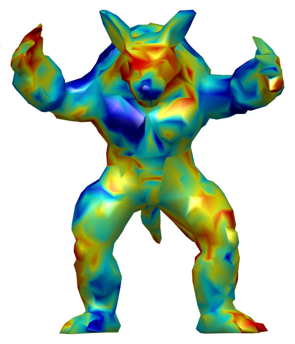
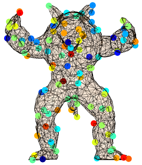
Figure 1: An example of graph completion on Armadillo mesh, given edge weights based on curvature. Left: noisy signal on the mesh, Middle: partial observation on the signal, Right: recovery of the signal on the mesh.

Key Ideas. The starting point of our proposed algorithm is to perform harmonic analysis on the given graph. Similar to the “low rank” property (for matrix completion), we also make use of parsimony/sparsity, albeit in terms of representations obtained in the Fourier/wavelet space of the graphs. Recall that measurements/signals are represented as a smooth function in their graph space but their representations in a dual space may be sparse, which is an important advantage of the frequency analysis [20]. We exploit a similar idea, in the graph setting using the graph Fourier transform. The “online” version of the completion problem is defined using the frequency space of this graph. When we acquire a measurement on a vertex, the “value of information” for the remaining set of unobserved vertices changes to impact our “policy” to acquire the next measurement. This strategy is related to the idea of diminishing returns but is an “adaptive” variation. While such an online scenario has been studied for a general matrix or tensor setting [21, 22, 25], no algorithms are available for graphs. We show how recent work on submodular maximization can be adapted for analysis of measurements on a graph in this online manner utilizing the graph Fourier representation.

In this paper, we provide a framework for deciding the optimal policy of selecting vertices on a graph for an accurate and efficient recovery of a signal by exploring its dual representation. The contributions of this paper are: 1) we propose an algorithm for sequentially selecting vertices on a graph using adaptive submodularity, 2) we provide an algorithm for sequentially recovering signals on graph vertices using the graph Fourier transform, 3) we demonstrate extensive results on large-scale image datasets as well as a neuroimaging dataset. On the image data, we estimate object labels on images where state-of-the-art object detectors fail. On the neuroimaging data, we estimate expensive summary measures from brain scans using other cheaper measures.

2 Background: Fourier and Wavelet Transforms in Non-Euclidean Spaces

The Fourier and wavelet transforms have been extensively studied almost exclusively in Euclidean spaces. Recently, several groups have demonstrated the analogs of these transforms in non-Euclidean spaces [8, 14], which are fundamental for our proposed algorithm. We therefore provide a brief description in this section.

2.1 Fourier and Wavelet Transforms

The Fourier transform transforms a signal $f(x)$ in $x$ to $\hat{f}(\omega)$ in the frequency space $\omega$ using $\sin()$ basis functions as $\hat{f}(\omega)=\langle f,e^{j\omega x}\rangle=\int f(x)\mathrm{e}^{-j\omega x}\mathrm{d}x$. The concept underlying the wavelet transform is similar but it utilizes a localized oscillating basis function (i.e., mother wavelet) for the transform. While the Fourier basis has an infinite support, a wavelet $\psi$ is localized in both time and frequency space [26]. A mother wavelet with scale $s$ and translation $a$ parameters is written as $\psi_{s,a}(x)=\frac{1}{s}\psi(\frac{x-a}{s})$, where changing $s$ and $a$ varies the dilation and location of $\psi_{s,a}$ respectively. Using $\psi_{s,a}$ as basis, a wavelet transform of a function $f(x)$ yields wavelet coefficients $W_{f}(s,a)$ defined as

$$\small W_{f}(s,a)=\langle f,\psi\rangle=\frac{1}{s}\int f(x)\psi^{*}(\frac{x-a}{s})\mathrm{d}x$$ (1)

where $\psi^{*}$ is the complex conjugate of $\psi$.

In the frequency space, $\psi_{s}$ behave as band-pass filters covering different bandwidths corresponding to scales $s$. When these band-pass filters do not handle low-frequency bands, a scaling function $\phi$ (i.e., a low-pass filter) is introduced. In the end, a transform of $f$ with the scaling function $\phi$ results in a smooth representation of the original signal and filtering at multiple scales $s$ of the mother wavelet $\psi_{s}$ offers a multi-resolution view of the given signal. In both cases for the Fourier and wavelet transforms, there exist inverse transforms that reconstruct the original signal $f(x)$ using their coefficients and the basis functions.

2.2 Fourier and Wavelet Transforms for Graphs

The Euclidean space is typically represented as a regular lattice, therefore one can easily construct a mother wavelet with a certain shape to define a wavelet transform. On the other hand, in non-Euclidean spaces that are generally represented by a set of vertices and their arbitrary connections, the construction of a mother wavelet is ambiguous due to the definition of dilation and translation of $\psi_{s,a}$. Because of these issues, the classical Fourier/wavelet transform has not been suitable for analyzing data in complex space until recently when [14, 8] proposed these transforms for graphs.

The core idea for constructing a mother wavelet $\psi_{s}$ on the nodes of a graph comes from its representation in the frequency space. By constructing different shapes of band-pass filters in the frequency space and transforming them back to the original space, we can implement mother wavelets that maintain the traditional properties of wavelets. Such an implementation requires a set of “orthonormal” bases and a kernel (filter) function. The orthonormal bases span the analog of the frequency space in the non-Euclidean setting and the kernel function denotes the representation of $\psi_{s}$ in the frequency space. In this sense, when the non-Euclidean space is represented as a graph, we can adopt spectral graph theory [7] for orthonormal bases and design a $g()$ in the space spanned by the bases.

In general, a graph $\mathit{G}=\{V,E\}$ is represented by a set of vertices $V$ of size $N$ and a set of edges $E$ that connects the vertices. An adjacency matrix $\mathit{A}_{N\times N}$ is the most common way to represent a graph $\mathit{G}$ where each element $a_{ij}$ denotes the connection in $E$ between the $i$th and the $j$th vertices by a corresponding edge weight. Another matrix, a degree matrix $\mathit{D}_{N\times N}$, is a diagonal matrix where the $i$th diagonal element is the sum of edge weights connected to the $i$th vertex. From these two matrices, a graph Laplacian is then defined as $\mathit{L}=\mathit{D}-\mathit{A}$. Note that $\mathit{L}$ is a self-adjoint and positive semi-definite operator, therefore provides pairs of eigenvalues $\lambda_{l}\geq 0$ and corresponding eigenvectors $\chi_{l}$, $l=1,\cdots,N$ which are orthonormal to each other. The bases $\chi$ can be used to define the graph Fourier transform of a function $f(n)$ defined on the vertices $n$ as

$$\small\hat{f}(l)=\sum_{n=1}^{N}f(n)\chi^{*}_{l}(n)~{}~{}~{}\mbox{and}~{}~{}~{}f(n)=\sum_{l=1}^{N}\hat{f}(l)\chi_{l}(n)$$ (2)

where $\chi^{*}$ is a conjugate of $\chi$. Here, the graph Fourier coefficient $\hat{f}(l)$ is obtained by the forward transform and the original function $f(n)$ can be reconstructed by the inverse transform. If a signal $f(n)$ lives in the spectrum of the first $k$ eigenvectors, we say that $f(n)$ is $k$-bandlimited. This transform offers a way to look at a signal defined on graph vertices in a dual space which is an analog of the frequency space in the Fourier transform.

A mother wavelet $\psi$ then can be defined using the graph Fourier transform. First, a kernel function $g:\mathbb{R}^{+}\rightarrow\mathbb{R}^{+}$ (i.e., band-pass filter) is designed in the dual space, then this operation is localized by an impulse function $\delta_{n}$ at vertex $n$:

$$\footnotesize\psi_{s,n}(m)=\sum_{l=1}^{N}g(s\lambda_{l})\chi_{l}^{*}(n)\chi_{l}(m).$$ (3)

Here, the scale parameter $s$ is independent from $\chi$ and defined inside of $g()$ using the scaling property of Fourier transform [32]. Examples of localized $\psi_{s}$ on a mesh are shown in Fig. 2 comparing with a $\chi_{3}$ (not localized).

The wavelet transform of a function $f(n)$ on graph vertices $n$ at scale $s$ then can be written using the bases $\psi$ defined as in (3), and it follows the conventional definition of the wavelet transform yielding wavelet coefficients $W_{f}(s,n)$ at scale $s$ and location $n$ as

$$\small W_{f}(s,n)=\langle f,\psi_{s,n}\rangle=\sum_{l=1}^{N}g(s\lambda_{l})\hat{f}(l)\chi_{l}(n).$$ (4)

This transform offers a multi-resolution view of a signal defined on graph vertices just like the traditional wavelet transform in the Euclidean space (e.g., pixels) by multi-scale filtering. Our method to be introduced shortly will use the graph Fourier transform and wavelets on graphs to formalize adaptive vertex selection strategy and graph completion.

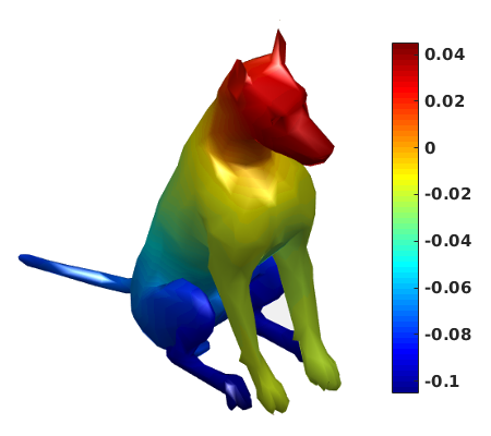
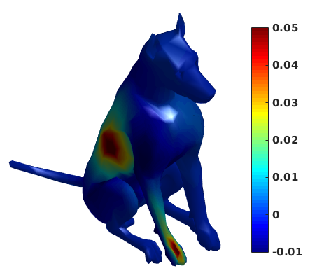
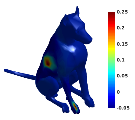
Figure 2: Examples of basis functions on a dog shaped mesh. Left: $\chi_{3}$ (not localized), Middle: two $\psi_{1}$ (localized) at the back and on a paw, Right: $\psi_{5}$ (localized and condensed).

3 Our Proposed Algorithm

Consider a setting where there exists an unknown bandlimited signal $f$ of $p$ features defined on $N$ graph vertices (in an identical state space). In other words, at each vertex $v$, we can in principle obtain a $p$-dimensional feature. However in reality, we may be able to observe the signal only at $m$$\ll$$N$ different vertices of the graph due to budget constraints. In this setting, there are two core questions we may ask related to the recovery of the signal $f$ at all vertices: 1) how to efficiently recover the signal on every vertex and 2) how to select the best $m$ vertices (and in which order) to acquire the additional measurements. We tackle these problems by formulating an adaptive submodular function derived from the frequency space of the graph. We provide our solutions to the two questions by showing that our formulation is adaptive submodular and proposing an algorithm to recover the full signal. Notice the distinction from classical active learning (also see [20, 21, 22]) that our specification is agnostic to the subsequent task (e.g., classification).

3.1 Signal Recovery in Graph Fourier Space

Suppose we have collected data from $m$ number of vertices $Y\in\mathbb{R}^{m\times p}$ from a full (unknown) function $f\in\mathbb{R}^{N\times p}$. Here, our objective is to recover the original signal $f$ based on the partial observation $Y$. We denote the set of selected indices as $W=\{w_{1},w_{2},\cdots,w_{m}\}$, and define a projection matrix $P$ that maps $f$ to $Y$ (i.e., $Pf=Y$):

$$\small P_{i,j}=\begin{cases}1~{}~{}~{}\text{if}~{}~{}~{}j=w_{i}\\ 0~{}~{}~{}\text{o.w.}\end{cases}.$$ (5)

Based on the data $Y$ from the selected data points (i.e., vertices), a naive signal recovery algorithms may solve for

$$\small Z^{*}=\operatorname*{arg\,min}_{Z\in\mathbb{R}^{N\times p}}||PZ-Y||_{\ell_{2}}^{2}$$ (6)

which minimizes the error between the observation and the estimation and typically used with a smoothness constraint. However, such a formulation operates in the native space of $\mathbb{R}^{N\times p}$ without utilizing the bandlimited property of signals. It can be also computationally challenging to deal with other constraints that requires full diagonalization of $\mathit{L}$. We therefore take this problem into its graph Fourier space using a set of orthonormal bases $U_{k}=[\chi_{1},\chi_{2},\cdots,\chi_{k}]$ and search for a solution in the dual space spanned by $U_{k}$. One of the most fundamental properties of the Fourier representation is its sparsity. In many cases, even a very dense form of signals in its original domain can be reconstructed with a few $\sin()$ functions. Signals in the image space tend to be smooth among pixels that are spatially close, on the other hand, their frequency representations are independent from such a spatial constraint [20]. Such an observation is crucial for methods for low-rank estimation of signal/measurement and has been utilized in machine learning and computer vision literature [6, 4]. In this regime, we would want to obtain a bandlimited solution that is sparse within the range of $k$-band. Transforming (6) into the space spanned by $U_{k}$ and imposing $\ell_{1}$-norm constraint for the sparsity, we obtain

$$\small\hat{Z}^{*}=\operatorname*{arg\,min}_{\hat{Z}\in\mathbb{R}^{k\times p}}||PU_{k}\hat{Z}-Y||_{\ell_{2}}^{2}+\xi||\hat{Z}||_{\ell_{1}}$$ (7)

where $\xi$ controls the sparsity and its solution is easily obtainable using a LASSO solver [34]. The optimal solution $\hat{Z}^{*}$ here is an estimation of sparse encoding of the original signal $f$ in the frequency space, and its representation in the original space can be empirically recovered by performing the inverse graph Fourier transform as $Z^{*}(n)=\sum_{l=1}^{k}\hat{Z}_{k}^{*}(l)\chi_{l}(n)$. Note that in (7), we avoid imposing a smoothness constraint that has been used in other approaches [28, 27], since our solution is already smooth due to its low-rank and bandlimited properties. However, the smoothness criteria may still be useful when our assumption (i.e., sparsity) in the dual domain does not hold.

3.2 Performing Adaptive Selection of Vertices

In order for our signal recovery process to obtain the best estimation possible, the optimal sequential selection of vertices to construct the projection matrix $P$ is critical. For this task, we approach this problem from an adaptive submodular perspective. Let us first clarify some notations to describe adaptive submodularity.

Given a set of vertices $V$ with possible states $S$, we denote a function $\gamma:V\rightarrow S$ as a realization. We also denote $\Gamma$ as a random realization with a prior probability $\mathbf{p}(\gamma):=\mathbb{P}[\Gamma=\gamma]$. Under this setting, we look for a strategy to select a vertex $v$, observe its state $\Gamma(v)$ and then select the next vertex conditioned on the previous observations. The set of observations until the most recent stage is represented as partial realization $\theta$ and its domain defined as $\operatorname*{dom}(\theta)=\{v|\exists o,(v,o)\in\theta\}$. The selection process defines a policy $\pi=\{\pi_{1},\pi_{2},\cdots\pi_{m}\}$ which is an ordered set of $m$ number of selected vertices. Given a policy $\pi$, a function $f:2^{V}\times O^{V}\rightarrow\mathbb{R}$ depends on the selection of vertices and its states. Defining $V(\pi,\Gamma)$ as the set of vertices under realization $\Gamma$, we can formulate a problem to identify the optimal strategy with $f_{avg}=\mathbb{E}[f(V(\pi,\Gamma)),\Gamma]$ as

$$\small\pi^{*}\in\operatorname*{arg\,max}_{\pi}f_{avg}(\pi)\text{~{}~{}s.t.~{}~{}}|V(\pi,\Gamma)|\leq k$$

that is known as adaptive stochastic maximization problem [13]. With conditional expected marginal benefit defined as

$$\small\Delta(v|\theta)=\mathbb{E}[f(\operatorname*{dom}(\theta)\cup\{v\},\Gamma)-f(\operatorname*{dom}(\theta),\Gamma)|\Gamma],$$ (8)

it is known that a function $f:2^{V}\times S^{V}:\rightarrow\mathbb{R}$ is adaptive monotone when $\Delta(v|\theta)\geq 0$ and adaptive submodular when $\Delta(v|\theta)\geq\Delta(v|\theta^{\prime})$ with $\theta\subseteq\theta^{\prime}$ [13]. Such a problem is easily solved approximately by a greedy algorithm that maximizes $\Delta(v|\theta)$ at each iteration. For example, if the $V$ are potential locations to place certain sensors and $f()$ is a function that computes the area covered by the sensors, given a probability that some sensors fail at random (i.e., $\mathbf{p}(\gamma)$), one can maximize the total expected area covered by selected sensors by such an algorithm.

Such a setup can be computationally challenging due to the size of $V$ and requires an accurate prior probability. We therefore tackle our problem of selecting the vertices in a simpler manner by computing a “leverage value” that describes the importance of each vertex using frequency properties of a given graph. In our formulation, once a vertex is selected based on the leverage measure and data are acquired, then its state gets fixed (i.e., placed sensors do not fail). Notice that such a setting makes the problem deterministic. However, once we observe the state of the vertex and evaluate its contribution to the signal recovery process, we will adaptively modify the leverage value for all remaining vertices to make the next selection. That is, once a vertex is added to the policy $\pi$, we will perform our signal recovery process as described in section 3.1 to evaluate how well the signal is recovered at the newly selected vertex which will adaptively affect our next selection. In this setting, the conditional marginal benefit (no longer an expectation), given a policy $\pi$ is defined as

$$\small\Delta(v|\pi)=f(\operatorname*{dom}(\pi)\cup\{v\}|\pi)-f(\operatorname*{dom}(\pi)|\pi)$$ (9)

which is a specific case of (8) with a fixed policy $\pi$ instead of a random realization.

Next, in order to define our utility function, we define a measure that describes a notion of importance at each vertex. At each vertex, we can define the leverage value as

$$\small I(n)=\sum_{l=1}^{k}g(\lambda_{l})\chi_{l}(n)^{2}$$ (10)

which is a reconstruction of $\delta_{n}$ at vertex $n$ using $U_{k}$ and a kernel function $g()$ [31, 3, 1, 15, 19]. The leverage value $I(n)\geq 0$ describes how much energy is preserved at vertex $n$ at scale $s$ and roughly describes how well a signal can be recovered at each vertex with limited number of bases. In order for an accurate signal recovery on the selected vertices, we want to prioritize vertices with high $I$ when selecting a vertex $v$ for $\pi$. Moreover, we assume that the signals on neighboring vertices may be similar (i.e., smooth) and modulate down $I$s from neighboring vertices of $v$ when it gets selected. To define the notion of “closeness” between vertices, we use a diffusion-type distance [9, 18] defined as

$$\small D_{s,n^{\prime}}(n)=\sum_{l=1}^{k}g(s\lambda_{l})\chi_{l}(n^{\prime})\chi_{l}(n)$$ (11)

which measures how far a vertex $n$ and $n^{\prime}$ are at scale $s$ by an energy propagation process. Using these concepts, given $I^{j}$ after $j$ number of selections, the leverage value $I^{j+1}$ for the next selection is defined as

$$\small I^{j+1}=I^{j}-\eta_{j}D$$ (12)

where $\eta_{j}$ is a constant to set $I^{j+1}(\pi_{j})=0$. Notice that for the leverage values $I^{j}(v)$ and $I^{j+1}(v)$ on the same vertex $v$ at $j$ and $(j+1)$th iterations, $I^{j}(v)\geq I^{j+1}(v)$ with $D>0$. With the leverage value $I^{j}$ in hand, we define a utility function $f(\pi)=\sum_{i=1}^{|\pi|}I^{i}(\pi_{i})$ which is the sum of $I(\cdot)$ from each selection. Using the two results below, we show that our utility function is adaptive monotone and adaptive submodular and can be approximately solved in a greedy way.

Lemma 1.

Given current policy $\pi=\{\pi_{1},\pi_{2},\cdots,\pi_{j}\}$ of size $j$, $f(\pi)=\sum_{i=1}^{j}I^{i}(\pi_{i})$ is adaptive monotone.

Proof.

The conditional benefit of adding a vertex $v$ having observed $\pi$ is

$$\Delta(v|\pi) =f(\operatorname*{dom}(\pi)\cup\{v\}|\pi)-f(\operatorname*{dom}(\pi)|\pi)$$

$$=\sum_{i=1}^{j}I^{i}(\pi_{i})+I^{j+1}(v)-\sum_{i=1}^{j}I^{i}(\pi_{i})$$

$$=I^{j+1}(v)\geq 0$$

∎

This lemma shows that the benefit of adding a vertex $v$ is always non-negative and $f(\pi)$ follows the traditional definition of monotonicity (i.e., $f(A)\leq f(B)$ holds whenever $A\subseteq B$) with positive $I$.

Lemma 2.

Given two policies $\pi$ of size $j$ and $\pi^{\prime}$ of size $j^{\prime}$ where $\pi\subseteq\pi^{\prime}$, our utility function $f(\pi)=\sum_{i=1}^{j}I^{i}(\pi_{i})$ is adaptive submodular.

Proof.

The difference between the conditional benefits from the two observations (i.e., policies) $\pi$ and $\pi^{\prime}$ is

$$\Delta(v|\pi)-\Delta(v|\pi^{\prime}) =f(\operatorname*{dom}(\pi)\cup\{v\}|\pi)-f(\operatorname*{dom}(\pi)|\pi)$$

$$~{}~{}-(f(\operatorname*{dom}(\pi^{\prime})\cup\{v\}|\pi^{\prime})-f(\operatorname*{dom}(\pi^{\prime})|\pi^{\prime}))$$

$$=I^{j+1}(v)-I^{j^{\prime}+1}(v)\geq 0$$

∎

This result shows that the utility function $f(\pi)$ satisfies an adaptive analog of the traditional definition of submodularity [12] (i.e., $f(A\cup\{v\})-f(A)\geq f(B\cup\{v\})-f(B)$ when $A\subseteq B\subseteq V\text{~{}~{}and~{}~{}}v\in V\setminus B$) and it can be used to formulate an adaptive submodular optimization problem.

Given our adaptive submodular utility function at hand, we define this iterative process as Select and Recover (SR) method by formulating the following problem:

$$\pi^{*}\in ~{}\operatorname*{arg\,max}_{\pi}~{}~{}\sum_{i=1}^{j}I^{i}(\pi_{i})$$ (13)

$$s.t.~{}~{}I^{i+1}=I^{i}-\eta_{i}D,~{}j\leq m.$$

Such an adaptive submodular problem is solved by a greedy algorithm that comes with performance guarantees [13].

Once we obtain the the optimal $\pi^{*}$, we can finalize a set of selected vertices $W$ and a projection matrix $P$ which are the key ingredients for our signal recovery step. Using $W$, we go through the process as described in section 3.1 and obtain the estimation of the unknown signal. This whole pipeline is summarized in the Algorithm 1 below, where we solve LASSO at each iteration which is easily scalable.

1

Input : vertex set $V$, orthonormal bases $U_{k}$, total number of selection $m$ and $D$ update parameter $\alpha$

Output : $Z$: recovered signal

2 $\pi\leftarrow\emptyset$, $s\leftarrow 0$

3 Derive $I^{1}(n)$ using $U_{k}$ as in (10)

4 for $i=1\text{\bf~{}~{}to~{}~{}}m$ do

5       Selection step: $v^{*}=\operatorname*{arg\,max}_{v}\Delta(v|\pi)$

6       $\pi\leftarrow\pi\cup\{v^{*}\}$

7       Observe $f(\operatorname*{dom}(\pi))$

8       Recovery step: obtain $Z^{*}$ as in section 3.1

9       $s\leftarrow\alpha|f(\pi_{i})-Z^{*}(\pi_{i})|$

10       $I^{i+1}\leftarrow I^{i}-\eta_{i}D_{s}$

11 end for

Return $Z^{*}$

Algorithm 1 Select and Recover (SR) Method

4 Experimental Results

In this section, we demonstrate various experimental results using our framework on three different datasets. The first unique dataset consists of images and comments that we collected from Imgur (http://www.imgur.com), where we qualitatively evaluate our framework for labeling objects in images where object detectors failed. The second dataset is publicly available MSCOCO, where we make quantitative evaluations for a multi-label learning problem with human-specified object labels. The basic schematic of how the SR method works on these datasets is shown in Fig. 3. The last experiment focuses on Alzheimer’s disease (AD) image dataset that consist of participants with Pittsburgh compound B positron emission tomography (PIB-PET) scans and Cerebrospinal fluid (CSF) data. Here, we use the CSF measures and SR method to predict PIB imaging measures where CSF data is much cheaper to acquire.

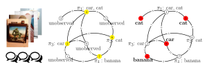
Figure 3: Our workflow on image datasets. Left: images and text, Middle: a graph derived from the text and a policy $\pi$ (yellow vertices), Right: recovered object labels on unobserved vertices (red vertices).

4.1 Object Label Estimation over Object Detection

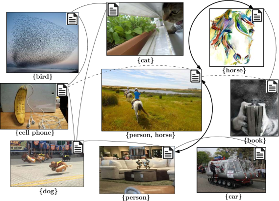
Figure 4: Various results on object label estimation from our Imgur experiment. YOLO did not confidently assign any labels on these images (i.e., below 40% confidence) using our 75 categories. However, our framework suggested that there were some objects in these image. The images represent nodes and the lines denote edges in our framework, and there are strong relationships between images with same object labels.

Dataset. We used MSCOCO categories to select a subset of categories on Imgur which provided images and comments, which gave us an interesting dataset to evaluate our algorithm. For each image, we obtained the top 10 comments upvoted by the community. We also created a dictionary of most commonly used words on Imgur (e.g., upvoted and downvoted) which were removed from the comments. We removed those categories that provided no images and the images with fewer than 10 comments. Our eventual dataset consisted of 10K images with 75 categories.

Setup. A graph of 10K vertices (i.e., images) with total of 49995k edges was generated by calculating the pairwise similarity between the comments from each image. To compute the similarities, the comments were first cleaned (i.e., removing stopwords, URLs and non-alphabetical letters) using natural language toolkit (NLTK) [2] and vector embedding using Word2Vec [30]. Then, the sanitized comments were used to compute Word’s Mover’s Distance (WMD) [23] using HTCondor distributed computing software. In our case, the WMD ranged in $(4,16)$ and we used a Gaussian kernel to transform the WMD into similarity measure within $(0,1)$. In order to assign object labels in each image, we used You Only Look Once (YOLO) [29], a deep learning framework pretrained on MSCOCO images and categories. After thresholding the confidence level at $40\%$, we ended up with 6329 images with at least one label.

We applied SR framework (using $\alpha=1$ and $\xi=0.01$) on this graph with the object labels as measurements on the vertices as in Fig. 3. Note that our framework works in an online manner. We first select a vertex (i.e., an image) $\pi_{1}$ and obtain corresponding image labels as in section 3.2 and then run the recovery process as in section 3.1 which will inform how the next vertex $\pi_{2}$ should be selected. After running this procedure $m$ times until $\pi_{m}$, we obtain our policy $\pi$ to be used for final image label recovery. We will demonstrate our results with $m=50\%$ of the total samples, i.e., selection of $5000$ (of 10K) vertices to obtain image labels and perform estimation over all vertices including the $5000$ vertices where our model has not obtained a measurement (class/object label). Note that we do not have ground truth (i.e., true object labels) for this dataset. We therefore show various interesting qualitative results on the images where YOLO did not detect objects with high confidence.

Results. Our representative results on object label estimation on the unselected images are demonstrated in Fig. 4. Note that we were not able to assign any labels for objects in these images using YOLO, since these objects were severely occluded/scaled, not in traditional shape or artificial objects. However, our framework successfully suggested labels for some of the unlabeled images with our 75 predefined categories. For the images where both YOLO and our method did not yield any labels, post-hoc analysis suggested that many of these images contained little visual context. More results are shown in the appendix.

Figure 5: Examples of images where our method assigns false labels. We assigned car for body shop (left), sheep instead of sheep shaped chair (middle) and person instead of a person shaped apple (right).

There were some failure cases where our method assigned false labels that generally falls in one of the following cases: 1) SR predicted “persons” but only a small part of a person (e.g., hand, arm or finger) was seen, 2) SR detected objects that had images of texts describing the object, 3) similar/related objects exist in the image but not exact (e.g., car center labeled as ‘car’). Some of these examples which are still interesting are shown in Fig. 5.

4.2 Multi-label Learning on MSCOCO Dataset

Dataset. We used the MSCOCO dataset where $\sim$$328000$ images with $82$ different object categories and relevant captions were available [24]. We retrieved the first 80 images from $80$ different categories and their corresponding captions to generate a smaller dataset to evaluate our SR method. When overlapping images between categories were discarded, our dataset included $5440$ images.

Setup. A graph using MSCOCO data was generated based on the captions from the $5440$ images (i.e., $5440$ nodes). The edges were defined using WMD in the same way as in section 4. Measurements at each vertex were given as a binary $1\times 80$ vector representing object labels where non-zero elements indicate whether the corresponding objects exist in the image. Concatenating $5440$ of them, we get a $f_{5440\times 80}$ matrix which served as the ground truth. Depending on the sampling ratio, $m$ number of rows of the matrix were selected according to our policy $\pi$ to obtain object labels, and we recovered the measurements on all rows. Notice that the ground truth labels are skewed, i.e., 0s dominates over 1s since there are only a few objects in each image. Therefore, to evaluate our algorithm, we computed the number of errors that SR makes as well as mean precision of the prediction. We compared our results with two other baseline methods 1) Puy et a.l [27] and 2) Rao et al. [28], which are the state-of-art methods for graph completion. For the signal recovery step, we used $\alpha=1$, $\xi=0.01$ and only $60\%$ of the total bases in our algorithm for estimation while other methods required all of them.

Result. After recovering the object labels for all images, we thresholded the estimation at $0.15$ to make the recovered labels binary (i.e., 1 if a recovered signal is $>0.15$ and 0 otherwise). Since baseline methods are stochastic, we ran them 100 times and computed the mean of evaluation scores with optimzed parameters. Table 1 shows the number of mistakes (out of 435200 estimations) with respect to the size of our policy (or the total number of samples). As the number of samples that we select increases, the errors decrease in all three methods and our method makes the fewest errors.

Sampling	Ours (SR)	Puy et al.	Rao et al.
$20\%$	19531	21274.6	23992.6
$30\%$	17246	19503.3	20427.7
$40\%$	15003	17862.2	17762.4
$60\%$	8992	10689.6	11906.9

Table 1: $\#$ of errors (out of 435200) in the recovered measurements

We also report mean precision over all categories instead of accuracy in Fig. 6. Here, the precision increases as the size of the policy increases and our result shows higher precision than those from the baselines as well as in [20] reaching up to $0.84$ with $60\%$ of total vertices.

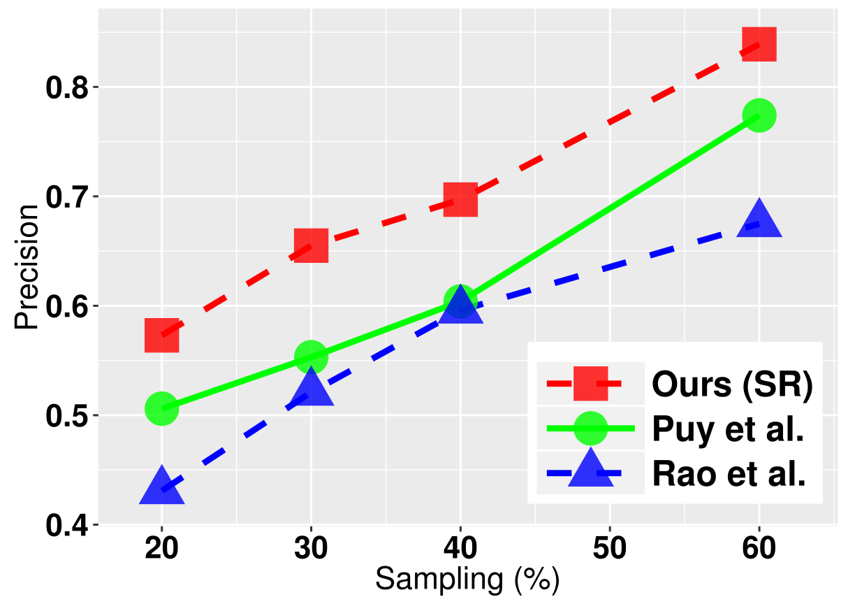
Figure 6: Mean precision over all categories w.r.t sampling ratio. As the number of samples increase, precision increases. SR (red) shows higher precision than Puy et al (green) and Rao et al (blue) at all sampling rates.

4.3 Estimation of PIB Measures using CSF

Dataset. Our AD dataset includes 79 participants where both PIB-PET scans and CSF are available. The voxel intensities of PIB-PET scans measure amyloid plaque pathology in the brain which is highly related to brain function as do the CSF measures, and these two measures are known to be highly (negatively) correlated [11]. We parcellated the brain into multiple regions of interests (ROI) and took the mean of the PIB measures in 16 selected ROIs to obtain ROI specific PIB measures. From the CSF data, we obtained various protein levels for each participant. More details of the dataset are given in the appendix.

Setup. The PIB images and the CSF measures involve different costs where PET scans are much more expensive, and CSF measures are often acquired as a surrogate for PET scans. In this experiment, we try to estimate PET image-derived measures based on CSF measures from the full cohort and PET image-derived measures on a subset of participants. A graph using CSF measures from each participant (i.e., vertex) was created by measuring similarity (i.e., edge) between participants using a Gaussian kernel $\exp(-(x-y)^{2}/\sigma^{2})$ with $\sigma=1$. Then we applied our framework as in Alg. 1 to decide a policy to obtain PIB imaging measures from $v\in\pi$ on the 16 ROIs and recover the measures over all (remaining) participants. We used $\xi$$=$$0.01$ for the sparsity parameter, $k$$=$$50$ number of eigenvectors and $\alpha$$=$$1$ for the signal recovery step.

Result. We show the $\ell_{2}$-norm of the error between the ground truth and the recovered measures for evaluation. Again, we ran the baseline methods $500$ times to compute the mean of errors due to their stochasticity. We ran the experiments by varying $m$ and reported the results with $m=\{30\%,50\%\}$ of the total samples. As summarized in Fig. 7, our result (in red) shows much lower error than the baseline methods. When we used these estimation results to identify whether each participants had elevated amyloid burden (i.e., whether mean of PIB measures over all ROIs is $>1.18$), our estimation offered $91.1\%$ accuracy while [27] and [28] provided $88.6\%$ and $87.6\%$.

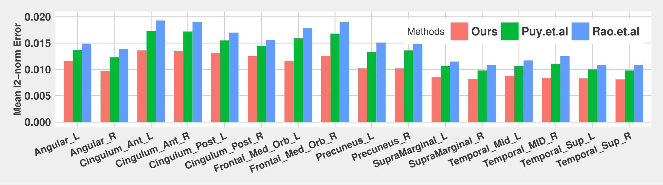
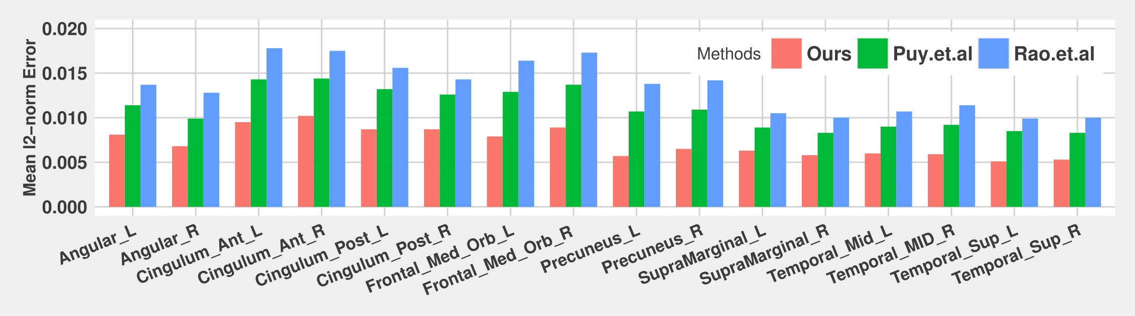
Figure 7: ROI-wise mean $\ell_{2}-$norm error between recovered signals and the ground truth using SR (red), Puy et al.(green) and Rao et al.(blue). Top: using $30\%$ of the total samples, Bottom: using $50\%$ of the total samples.

5 Conclusion

Motivated by various instances in modern computer vision that involve an interplay between the data (or supervision) acquisition and the underlying inference methods, we study the problem of adaptive completion of a multivariate signal obtained sequentially, on the vertices of graph. By expressing the optimization in the frequency domain of the graph, we show how a simple algorithm based on adaptive submodularity yields impressive results across diverse applications. On large-scale vision datasets, our proposal complements object detection algorithms by solving a completion problem (using auxiliary information). The model provides promising evidence how neuroimaging studies under budget constraints can be conducted (in a sequential manner) with minimal deterioration in statistical power. Our open source distribution will enable applications to other settings in vision which involves partial measurements and/or sequential observations of data structured as a graph.

6 Acknowledgement

This research was supported by NIH grants AG040396, AG021155, EB022883, NSF CAREER award 1252725, UW ADRC AG033514, UW CIBM 5T15LM007359-14, and UW CPCP AI117924.

References

- [1] M. Aubry, U. Schlickewei, and D. Cremers. The wave kernel signature: A quantum mechanical approach to shape analysis. In ICCV Workshops, pages 1626–1633. IEEE, 2011.
- [2] S. Bird, E. Klein, and E. Loper. Natural language processing with Python. ” O’Reilly Media, Inc.”, 2009.
- [3] M. M. Bronstein and I. Kokkinos. Scale-invariant heat kernel signatures for non-rigid shape recognition. In CVPR, pages 1704–1711. IEEE, 2010.
- [4] J.-F. Cai, E. J. Candès, and Z. Shen. A singular value thresholding algorithm for matrix completion. SIAM Journal on Optimization, 20(4):1956–1982, 2010.
- [5] E. J. Candes and Y. Plan. Matrix completion with noise. Proceedings of the IEEE, 98(6):925–936, 2010.
- [6] E. J. Candès and B. Recht. Exact matrix completion via convex optimization. Foundations of Computational mathematics, 9(6):717–772, 2009.
- [7] F. R. Chung. Spectral graph theory, volume 92. AMS Bookstore, 1997.
- [8] R. Coifman and M. Maggioni. Diffusion wavelets. Applied and Computational Harmonic Analysis, 21(1):53 – 94, 2006.
- [9] R. R. Coifman and S. Lafon. Diffusion maps. Applied and Computational Harmonic Analysis, 21(1):5–30, 2006.
- [10] D. L. Donoho. Compressed sensing. IEEE Transactions on information theory, 52(4):1289–1306, 2006.
- [11] A. M. Fagan, M. A. Mintun, R. H. Mach, , et al. Inverse relation between in vivo amyloid imaging load and cerebrospinal fluid a42 in humans. Annals of Neurology, 59(3):512–519, 2006.
- [12] S. Fujishige. Submodular functions and optimization, volume 58. Elsevier, 2005.
- [13] D. Golovin and A. Krause. Adaptive submodularity: Theory and applications in active learning and stochastic optimization. Journal of Artificial Intelligence Research, 42:427–486, 2011.
- [14] D. Hammond, P. Vandergheynst, and R. Gribonval. Wavelets on graphs via spectral graph theory. Applied and Computational Harmonic Analysis, 30(2):129 – 150, 2011.
- [15] N. Hu, R. M. Rustamov, and L. Guibas. Stable and informative spectral signatures for graph matching. In CVPR. IEEE, 2015.
- [16] H. Ji, C. Liu, Z. Shen, and Y. Xu. Robust video denoising using low rank matrix completion. In CVPR, pages 1791–1798, 2010.
- [17] K. I. Kim. Semi-supervised learning based on joint diffusion of graph functions and laplacians. In ECCV, pages 713–729. Springer, 2016.
- [18] W. H. Kim, B. B. Bendlin, M. K. Chung, et al. Statistical inference models for image datasets with systematic variations. In CVPR, pages 4795–4803. IEEE, 2015.
- [19] W. H. Kim, M. K. Chung, and V. Singh. Multi-resolution shape analysis via Non-euclidean wavelets: Applications to mesh segmentation and surface alignment problems. In CVPR, pages 2139–2146. IEEE, 2013.
- [20] W. H. Kim, S. J. Hwang, N. Adluru, et al. Adaptive signal recovery on graphs via harmonic analysis for experimental design in neuroimaging. In ECCV, pages 188–205. Springer, 2016.
- [21] A. Krishnamurthy and A. Singh. Low-rank matrix and tensor completion via adaptive sampling. In NIPS, pages 836–844, 2013.
- [22] S. Kumar, M. Mohri, and A. Talwalkar. Sampling methods for the Nyström method. JMLR, 13(1):981–1006, 2012.
- [23] M. J. Kusner, Y. Sun, N. I. Kolkin, and K. Q. Weinberger. From word embeddings to document distances. In ICML, pages 957–966, 2015.
- [24] T.-Y. Lin, M. Maire, S. Belongie, et al. Microsoft coco: Common objects in context. In ECCV, pages 740–755. Springer, 2014.
- [25] Z. Lin, R. Liu, and Z. Su. Linearized alternating direction method with adaptive penalty for low-rank representation. In NIPS, pages 612–620, 2011.
- [26] S. Mallat. A wavelet tour of signal processing. Academic press, 1999.
- [27] G. Puy, N. Tremblay, R. Gribonval, et al. Random sampling of bandlimited signals on graphs. Applied and Computational Harmonic Analysis, 2016.
- [28] N. Rao, H.-F. Yu, P. K. Ravikumar, et al. Collaborative Filtering with Graph Information: Consistency and Scalable Methods. In NIPS, 2015.
- [29] J. Redmon, S. Divvala, R. Girshick, and A. Farhadi. You only look once: Unified, real-time object detection. arXiv preprint arXiv:1506.02640, 2015.
- [30] R. Řehůřek and P. Sojka. Software Framework for Topic Modelling with Large Corpora. In Proceedings of the LREC 2010 Workshop on New Challenges for NLP Frameworks, pages 45–50. ELRA, May 2010.
- [31] R. M. Rustamov. Laplace-Beltrami eigenfunctions for deformation invariant shape representation. In Eurographics Symposium on Geometry Processing, pages 225–233. Eurographics Association, 2007.
- [32] S.Haykin and B. V. Veen. Signals and Systems. Wiley, 2005.
- [33] J. Tang, R. Hong, S. Yan, T.-S. Chua, G.-J. Qi, and R. Jain. Image annotation by k-NN sparse graph-based label propagation over noisily tagged web images. ACM TIST, 2(2):14, 2011.
- [34] R. Tibshirani. Regression shrinkage and selection via the LASSO. Journal of the Royal Statistical Society. Series B (Methodological), pages 267–288, 1996.
- [35] S. D. Weigand, P. Vemuri, H. J. Wiste, et al. Transforming cerebrospinal fluid A42 measures into calculated Pittsburgh Compound B units of brain A amyloid. Alzheimer’s & Dementia, 7(2):133–141, 2011.
- [36] H. Yang, J. T. Zhou, and J. Cai. Improving multi-label learning with missing labels by structured semantic correlations. In ECCV, pages 835–851. Springer, 2016.
- [37] K. Yu, S. Zhu, J. Lafferty, et al. Fast nonparametric matrix factorization for large-scale collaborative filtering. In SIGIR, pages 211–218. ACM, 2009.