∎
Fidelity-susceptibility analysis of the honeycomb-lattice Ising antiferromagnet under the imaginary magnetic field
Abstract
The honeycomb-lattice Ising antiferromagnet subjected to the imaginary magnetic field with the “topological” angle and temperature was investigated numerically. In order to treat such a complex-valued statistical weight, we employed the transfer-matrix method. As a probe to detect the order-disorder phase transition, we resort to an extended version of the fidelity , which makes sense even for such a non-hermitian transfer matrix. As a preliminary survey, for an intermediate value of , we investigated the phase transition via the fidelity susceptibility . The fidelity susceptibility exhibits a notable signature for the criticality as compared to the ordinary quantifiers such as the magnetic susceptibility. Thereby, we analyze the end-point singularity of the order-disorder phase boundary at . We cast the data into the crossover-scaling formula with scaled carefully. Our result for the crossover exponent seems to differ from the mean-field and square-lattice values, suggesting that the lattice structure renders subtle influences as to the multi-criticality at .
1 Introduction
The concept of fidelity has been developed in the field of the quantum dynamics Uhlmann76 ; Jozsa94 ; Peres84 ; Gorin06 . The fidelity is given by the overlap between the ground states, and , with the proximate interaction parameters, and , respectively; see Refs. Vieira10 ; Gu10 ; Dutta15 for a review. Meanwhile, it turned out that it detects the quantum phase transitions rather sensitively Quan06 ; Zanardi06 ; HQZhou08 ; Yu09 ; You11 ; Mukherjee11 ; Rossini18 . Actually, the fidelity susceptibility (: number of lattice points) exhibits a pronounced signature for the criticality as compared to the ordinary quantifiers such as the magnetic susceptibility Albuquerque10 . Additionally, the fidelity susceptibility does not rely on any presumptions as to the order parameter concerned Wang15 , and it is less influenced by the finite-size artifacts Yu09 . As would be apparent from the definition, the fidelity fits the numerical diagonalization method, which admits the ground-state vector explicitly. However, It has to be mentioned that the fidelity is accessible via the quantum Monte Carlo method Albuquerque10 ; Wang15 ; Schwandt09 ; Grandi11 and the experimental observations Zhang08 ; Kolodrubetz13 ; Gu14 as well.
In this paper, by the agency of the fidelity, we investigate the honeycomb-lattice Ising antiferromagnet under the imaginary magnetic field. To cope with the complex-valued statistical weight, we employed the transfer-matrix method Forcrand18 ; Zhou08 through resorting to the extended version of the fidelity Schwandt09 ; Sirker10
| (1) |
which makes sense even for such a non-hermitian transfer matrix. Here, the right and left eigenvectors and satisfy
| (2) |
and
| (3) |
respectively, with the maximal eigenvalue of the transfer matrix . Notably, the expression (1) reduces to the aforementioned one , provided that the matrix is hermitian, and the vectors are adjoint. In the present work, the matrix is non-symmetric and complex-valued, and it is by no means hermitian. So far, the real-non-symmetric Sirker10 and complex-valued-symmetric Forcrand18 ; Nishiyama20 transfer matrices were treated for the quantum chain and square-lattice Ising antiferromagnet under the imaginary field, respectively. In this paper, we demonstrate that the complex-valued non-symmetric , namely, the honeycomb-lattice case, is also tractable with the simulation scheme. It is anticipated that the criticality of the honeycomb-lattice model is not identical to that of the square-lattice model, because the former possesses the duality Imaoka96 ; Suzuki90 ; Lin88 at a finely-tuned value of the imaginary magnetic field.
To be specific, we present the Hamiltonian for the honeycomb-lattice Ising antiferromagnet subjected to the imaginary magnetic field
| (4) |
Here, the Ising spin is placed at each honeycomb-lattice point , and the summation runs over all possible nearest-neighbor pairs . Hereafter, the antiferromagnetic coupling constant is regarded as the unit of energy . The magnetic field takes a pure imaginary value
| (5) |
with the “topological” angle , and temperature , and likewise, the reduced coupling constant is introduced.
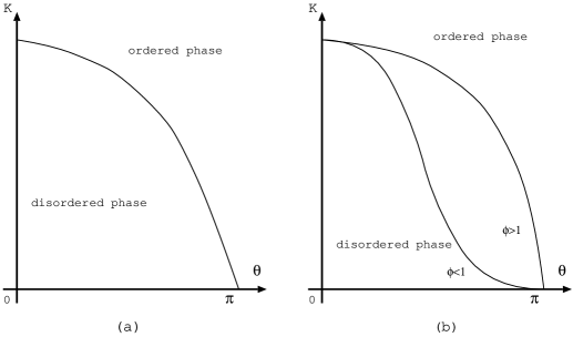
A schematic drawing of the phase diagram Imaoka96 ; Suzuki90 ; Lin88 ; Kim10 ; Matveev96 ; Matveev96b is presented in Fig. 1 (a). The order-disorder phase boundary extends into the finite- regime, and eventually, the phase boundary terminates at . So far, the model (4) has been investigated by means of the partition-function zeros Kim10 , albeit with an emphasis on the real--driven criticality. Additionally, rigorous information in terms of the duality theory Imaoka96 ; Suzuki90 ; Lin88 ; Matveev96 ; Matveev96b is available at . In fairness, it has to be mentioned that the square-lattice counterpart has been investigated with the partition-function-zeros Matveev08 , series-expansion Azcoiti17 , and exact-diagonalization Nishiyama20 methods in order to surmount the severe sign problem due to the imaginary magnetic field Azcoiti11 . In particular, the series expansion has played a significant role; actually, the above-mentioned works, Ref. Matveev96 and Azcoiti17 , made use of the low-temperature and cumulant expansions, respectively, elucidating the underlying criticality rather systematically. The phase diagram, Fig. 1 (a), should resemble that of the square-lattice model in overall characters. In contrast, the ferromagnetic counterpart does exhibit no phase transition in the finite- domain according to the celebrated theory of the Lee-Yang zeros Lee52 .
Then, there arises a problem how the phase boundary ends up at ; see Fig. 1 (b). The mean-field result Azcoiti11 shows that the phase boundary is curved convexly around , characterized Riedel69 ; Pfeuty74 by the crossover exponent . On the contrary, the above mentioned numerical results Matveev08 ; Azcoiti17 ; Nishiyama20 for the square-lattice model indicate a concavely-curved phase boundary with . Because the honeycomb-lattice antiferromagnet at is under the reign of the duality theory Imaoka96 ; Suzuki90 ; Lin88 ; Matveev96 , the end-point singularity should reflect its peculiar characters. The aim of this paper is to explore quantitatively by casting the fidelity-susceptibility data into the crossover-scaling theory Riedel69 ; Pfeuty74 ; a key ingredient is that the probe exhibits a notable singularity at the end-point .
2 Numerical results
In this section, we present the numerical results for the honeycomb-lattice Ising antiferromagnet under the imaginary magnetic field (4). In order to cope with the complex-valued statistical weight, we employed the transfer-matrix method as developed in Ref. Forcrand18 , where the authors investigated the square-lattice version rather in detail; our simulation scheme owes to this development. In Fig. 2, we present a unit of the transfer-matrix slice for the honeycomb-lattice model. The row-to-row statistical weight between the spin arrangements, and (), yields the transfer-matrix element, . Here, we implemented the periodic-boundary condition such as and . As would be apparent from Fig. 2, the transfer matrix is not symmetric, , in contrast to that of the square-lattice case Forcrand18 . Correspondingly, in the present case, the left and right eigenvectors, and , are neither identical nor adjoint, and the extention of the fidelity (1) now becomes essential.
Provided that the fidelity (1) is at hand, we are able to evaluate the fidelity susceptibility
| (6) |
According to the scaling theory Albuquerque10 , the fidelity susceptibility (6) exhibits an enhanced singularity as compared to the ordinary quantifiers such as the magnetic susceptibility. Note that for the two-dimensional Ising antiferromagnet, both specific heat and uniform susceptibility exhibit weak (logarithmic) singularities at the Néel temperature. Hence, it is significant to search for alternative quantifiers so as to detect the signature for the criticality.
2.1 Finite-size-scaling analysis of the fidelity susceptibility (6) with the fixed
In this section, via the fidelity susceptibility (6), we investigate the order-disorder phase transition of the honeycomb-lattice antiferromagnet with an intermediate value of the imaginary magnetic field . At this point , a preceding simulation result Kim10 is available.
In Fig. 3, we present the approximate critical point for with the fixed and various system sizes . Here, the approximate critical point denotes the maximal point of the fidelity susceptibility
| (7) |
for each . The least-squares fit to these data yields an estimate in the thermodynamic limit . As a reference, we carried out the similar extrapolation scheme with the abscissa scale replaced with , and we arrived at an alternative estimate . The deviation between them dominates the least-squares-fitting error . Hence, regarding the former as a possible systematic error, we estimate the critical point as
| (8) |
The estimate (8) is to be compared with the preceeding result Kim10 ; see Table 1. In Ref. Kim10 , the distribution of the partition-function zeros was explored for the honeycomb-lattice antiferromagnet, albeit with an emphasis on the real--driven phase transition; afterward, we explain how the transition point was extracted from their simulation result. As presented in Table 1, our result [Eq. (8)] is comparable to this elaborated pioneering study, Kim10 . Such a feature validates the use of the -mediated simulation scheme even for the case of non-symmetric complex-valued transfer matrix of the honeycomb-lattice model (4).
We then turn to the analysis of the criticality, namely, ’s scaling dimension Albuquerque10 . Here, the index () denotes the fidelity-susceptibility (correlation-length) critical exponent such as (). In Fig. 4, the approximate critical exponent is plotted for with the fixed and various system sizes . Here, the approximate critical exponent is given by the logarithmic derivative of
| (9) |
for a pair of system sizes . The least-squares fit to these data yields an estimate in the thermodynamic limit . Alternatively, we arrive at with the abscissa scale replaced with . The deviation between them dominates the least-squares-fitting error . Hence, considering the former as a possible systematic error, we estimate the critical exponent as
| (10) |
According to the scaling theory Albuquerque10 , the scaling relation
| (11) |
holds with the magnetic-susceptibility critical exponent for the antiferromagnet . Putting our result [Eq. (10)] into this scaling relation (11), we obtain
| (12) |
This result indicates that the phase transition belongs to the two-dimensional-Ising universality class, (logarithmic) Fisher60 ; Kaufman87 .
A few remarks are in order. First, we stress that ’s scaling dimension, [Eq. (10)], is larger than that of the magnetic susceptibility, [Eq. (12)]. Therefore, the fidelity susceptibility admits a pronounced signature for the criticality as compared to the ordinary quantifiers such as the magnetic susceptibility. Such a feature is significant for the two-dimensional Ising antiferromagnet, where both specific heat and magnetic susceptibility exhibit weak (logarithmic) singularities at the Néel temperature. Last, we explain how the critical point was extracted from Fig. 2 (d) of Ref. Kim10 . In Ref. Kim10 , the partition-function zeros were calculated for the complex domain of with generic ; here, the reduced coupling constant is fixed to . In Fig. 2 (d) of Ref. Kim10 , the accumulation of zeros forms a branch, which is about to touch the unit circle (). Such a feature indicates that the -driven phase transition occurs at this crossing point. More specifically, we read off a couple of partition-function zeros and , and found that the line defined by these points crosses the unit circle at . The above data are tabulated in Table 1. Nonetheless, we stress that the mechanism behind the phase transition differs from that of the ferromagnetic case Lee52 , as noted in Ref. Kim10 . In the ferromagnetic case, the partition-function zeros simply forms a unit circle. Neither extra branch nor mutual crossing occurs, and no -driven phase transition takes place at all.
2.2 Scaling plot for with the fixed
In this section, in order to check the validity of the scaling analyses in Sec. 2.1, we present ’s scaling plot, which also sets a basis of the subsequent crossover-scaling analyses. The fidelity susceptibility obeys the scaling formula Albuquerque10
| (13) |
with ’s scaling dimension and a non-universal scaling function .
In Fig. 5, we present the scaling plot, -, for various system sizes () , () , and () with the fixed . Here, we made a proposition (two-dimensional-Ising universality), and the other scaling parameters are set to [Eq. (8)], and [Eq. (10)]. The scaled data in Fig. 5 collapse into the scaling function satisfactorily, validating the scaling analyses in Sec. 2.1 as well as the proposition . Hence, recollecting [Eq. (12)], we confirm that the order-disorder phase transition indeed belongs to the two-dimensional-Ising universality class.
The scaling plot, Fig. 5, indicates that the fidelity susceptibility is less affected by the finite-size artifact Yu09 . Such a feature is favorable for the exact diagonalization method, with which the tractable system size is rather restricted. Encouraged by this observation, we proceed to examine how the order-disorder phase boundary terminates at the extremum point .
2.3 Crossover-scaling plot for around
In the above section, based on the scaling formula (13), we confirmed that the order-disorder-phase-transition branch belongs to the two-dimensional Ising universality class. In this section, by the agency of , we further explore the end-point singularity of the phase boundary toward . For that purpose, introducing yet another controllable parameter and the accompanying crossover exponent , we consider the crossover-scaling formula Riedel69 ; Pfeuty74
| (14) |
with the -dependent critical point , and a non-universal scaling function . Here, the indices, and , are ’s scaling dimension and correlation-length critical exponent, respectively, right at . As in Eq. (13), the index satisfies Albuquerque10 with the fidelity-susceptibility critical exponent at .
As explained in Sec. 1, the crossover exponent describes the shape of the phase boundary as Riedel69 ; Pfeuty74 . Hereafter, the crossover exponent is considered as an adjustable parameter, and the other indices, , , and , are fixed in prior to the scaling analyses as follows. According to the duality theory Imaoka96 , the hexagonal-lattice Ising antiferromagnet at reduces to the triangular-lattice antiferromagnet, and the uniform-susceptibility and correlation-length exponents are given by and , respectively Horiguchi92 . Notably enough, through the duality, the frustrated (non-bipartite lattice) antiferromagnet comes out from the seemingly non-frustrated magnet, albeit with the imaginary magnetic field mediated. This is a peculiarity of the imaginary-field magnet, and such a character would not be captured properly by the mean-field treatment. These indices together with the relation Albuquerque10 (see Eq. (11)) immediately admit , which now completes the prerequisite for the crossover-scaling analysis.
In Fig. 6, we present the crossover-scaling plot, -, for various system sizes, () , () , and () . Here, the second argument of the scaling function is fixed to a constant value, , with an optimal crossover exponent , and the critical point was determined with the same scheme as that of Sec. 2.1. The crossover-scaled data in Fig. 6 collapse into a scaling curve; particularly, the data, () and () , are about to overlap each other, showing a tendency to the convergence as . Likewise, in Fig. 7 and 8, we present the crossover-scaling plot, -, with the crossover exponent, and , respectively; the symbols are the same as those of Fig. 6. Here, the second argument of the scaling function is set to and in the respective analyses. In the former (latter) scaling plot, the left- (right-) side slope starts to split off, indicating that even larger (smaller) parameter leads a scatter of the scaled data. Hence, considering that these parameters set the tolerable bounds, we estimate the crossover exponent as
| (15) |
This is a good position to address a number of remarks. First, the underlying physics behind the crossover-scaling plot, Fig. 6, differs from that of the fixed- scaling plot, Fig. 5. Actually, the former scaling dimension is much larger than the latter , and hence, the data collapse of the crossover-scaling plot is by no means accidental. Second, the honeycomb-lattice Ising antiferromagnet enjoys the duality theory Imaoka96 so as to fix the critical indices such as and Horiguchi92 . Hence, it is anticipated that the crossover exponent [Eq. (15)] reflects the peculiarities of the honeycomb-lattice structure. Actually, the estimate [Eq. (15)] differs from the mean-field value Azcoiti11 , whereas it is slightly suppressed as compared to the square-lattice case, Nishiyama20 . Because the magnetic-susceptibility index for the honeycomb lattice Horiguchi92 is substantially smaller than that of the square lattice Matveev95 , it is reasonable that the multi-criticality depends on each lattice structure undertaken. Last, we mention a candidate for the quantifier other than the fidelity susceptibility. So far, the correlation length has played a significant role in the finite-size-scaling analyses. Actually, it is accessible via the diagonalization method Forcrand18 , provided that the second-largest eigenvalue of the transfer matrix is at hand. The correlation length has an advantage in that it has a fixed scaling dimension a priori. However, the second-largest eigenvalue is computationally demanding particularly for the non-hermitian transfer matrix, and this scheme was not accepted here.
3 Summary and discussions
The honeycomb-lattice Ising antiferromagnet (4) under the imaginary magnetic field was investigated with the transfer-matrix method Forcrand18 . As a probe to detect the phase transition, we utilized the extended version Schwandt09 ; Sirker10 of the fidelity (1), which makes sense even for such a non-symmetric complex-valued transfer matrix.
As a demonstration, we investigated the order-disorder phase transition for with the fidelity susceptibility (6). Our result [Eq. (8)] is comparable to that of the partition-function-zeros method, Kim10 , indicating that the probe detects the phase transition sensitively even in the presence of the imaginary magnetic field. Furthermore, we estimated ’s scaling dimension as [Eq. (10)]. Through resorting to the scaling relation (11), we estimated magnetic-susceptibility’s scaling dimension as [Eq. (12)]. This result indicates that the criticality belongs to the two-dimensional-Ising universality class, (logarithmic) Fisher60 ; Kaufman87 . We then turn to the analysis of the end-point singularity of the phase boundary toward . With scaled carefully, the data are cast into the crossover-scaling formula (14) Riedel69 ; Pfeuty74 . Thereby, we estimated the crossover exponent as [Eq. (15)]. This result differs from the mean-field value Azcoiti11 , whereas it is slightly suppressed as compared to that of the square-lattice model, Nishiyama20 . It would be intriguing that the lattice structure renders subtle influences as to the end-point singularity. Actually, the honeycomb-lattice antiferromagnet at is under the reign of the duality theory Imaoka96 ; Suzuki90 ; Lin88 ; Matveev96 , and it is anticipated that the end-point singularity reflect its peculiar characters.
According to Refs. Suzuki90 ; Matveev08 ; Sarkanch18 , even in the ferromagnetic side , there should occur a singularity for generic values of ; a notable point is that the transition is not the ordinary order-disorder phase transition Suzuki90 . According to the partition-function-zeros survey Matveev08 , the transition point should locate around at as for the square lattice. Because the fidelity-susceptibility-mediated analysis does not require any a priori settings as to the order parameter, it would provide valuable information even for such an exotic singularity. This problem is left for the future study.
Acknowledgment
This work was supported by a Grant-in-Aid for Scientific Research (C) from Japan Society for the Promotion of Science (Grant No. 20K03767).
Author contribution statement
Y.N. conceived the presented idea, and performed the numerical simulations. He analyzed the numerical data, and wrote up the manuscript.
| method | quantifier | |
|---|---|---|
| partition-function zeros Kim10 | accumulation of zeros | |
| transfer matrix (present work) | fidelity susceptibility |


References
- (1) A. Uhlmann, Rep. Math. Phys. 9 (1976) 273.
- (2) R. Jozsa, J. Mod. Opt. 41 (1994) 2315.
- (3) A. Peres, Phys. Rev. A 30 (1984) 1610.
- (4) T. Gorin, T. Prosen, T. H. Seligman, and M. Žnidarič, Phys. Rep. 435 (2006) 33.
- (5) V. R. Vieira, J. Phys: Conference Series 213 (2010) 012005.
- (6) S.-J. Gu, Int. J. Mod. Phys. B 24 (2010) 4371.
- (7) A. Dutta, G. Aeppli, B. K. Chakrabarti, U. Divakaran, T. F. Rosenbaum and D. Sen, “Quantum Phase Transitions in Transverse Field Spin Models: From Statistical Physics to Quantum Information” (Cambridge University Press, Cambridge, 2015)
- (8) H. T. Quan, Z. Song, X. F. Liu, P. Zanardi, and C. P. Sun, Phys. Rev. Lett. 96 (2006) 140604.
- (9) P. Zanardi and N. Paunković, Phys. Rev. E 74 (2006) 031123.
- (10) H.-Q. Zhou, and J. P. Barjaktarevic̃, J. Phys. A: Math. Theor. 41 (2008) 412001.
- (11) W.-C. Yu, H.-M. Kwok, J. Cao, and S.-J. Gu, Phys. Rev. E 80 (2009) 021108.
- (12) W.-L. You and Y.-L. Dong, Phys. Rev. B 84 (2011) 174426.
- (13) V. Mukherjee, A. Polkovnikov, and A. Dutta, Phys. Rev. B 83 (2011) 075118.
- (14) D. Rossini and E. Vicari, Phys. Rev. E 98 (2018) 062137.
- (15) A. F. Albuquerque, F. Alet, C. Sire, and S. Capponi, Phys. Rev. B 81 (2010) 064418.
- (16) L. Wang, Y.-H. Liu, J. Imriška, P. N. Ma, and M. Troyer, Phys. Rev. X 5 (2015) 031007.
- (17) D. Schwandt, F. Alet, and S. Capponi, Phys. Rev. Lett. 103 (2009) 170501.
- (18) C. De Grandi, A. Polkovnikov, and A. W. Sandvik, Phys. Rev. B 84 (2011) 224303.
- (19) J. Zhang, X. Peng, N. Rajendran, and D. Suter, Phys. Rev. Lett. 100 (2008) 100501.
- (20) M. Kolodrubetz, V. Gritsev, and A. Polkovnikov, Phys. Rev. B 88 (2013) 064304.
- (21) S.-J. Gu and W. C. Yu, Europhys. Lett. 108 (2014) 20002.
- (22) P. de Forcrand and T. Rindlisbacher, EPJ web of conferences 175 (2018) 07026.
- (23) H.-Q. Zhou, R. Orús, and G. Vidal, Phys. Rev. Lett. 100 (2008) 080601.
- (24) J. Sirker, Phys. Rev. Lett. 105 (2019) 117203.
- (25) Y. Nishiyama, arXiv:2005.10373.
- (26) H. Imaoka and Y. Kasai, J. Phys. Soc. Japan 65 (1996) 725.
- (27) M. Suzuki, J. Phys. Soc. Japan 60 (1990) 441.
- (28) K. Y. Lin and F. Y. Wu, Int. J. Mod. Phys. B 2 (1988) 471.
- (29) S.-Y. Kim, Phys. Rev. E 82 (2010) 041107.
- (30) V. Matveev and R. Shrock, J. Phys. A: Math. Theor. 29 (1996) 803.
- (31) V. Matveev and R. Shrock, Phys. Rev. E 53 (1996) 254.
- (32) V. Matveev and R. Shrock, J. Phys. A: Math. Theor. 41 (2008) 135002.
- (33) V. Azcoiti, G. Di Carlo, E. Follana, and E. Royo-Amondarain, Phys. Rev. E 96 (2017) 032114.
- (34) V. Azcoiti, E. Follana, and A. Vaquero, Nucl. Phys. B 851 (2011) 420.
- (35) T. D. Lee and C. N. Yang, Phys. Rev. 87 (1952) 410.
- (36) E.K. Riedel and F. Wegner, Z. Phys. 225 (1969) 195.
- (37) P. Pfeuty, D. Jasnow, and M. E. Fisher, Phys. Rev. B 10 (1974) 2088.
- (38) M. E. Fisher, Proc. R. Soc. London A 254 (1960) 66.
- (39) M. Kaufman, Phys. Rev. B 36 (1987) 3697.
- (40) T. Horiguchi, K. Tanaka, and T. Morita, J. Phys. Soc. Japan 61 (1992) 64.
- (41) V. Matveev and R. Shrock, J. Phys. A: Math. Theor. 28 (1995) 4859.
- (42) P. Sarkanych, Y. Holovatch, and R. Kenna, J. Phys. A: Math. Theor. 51 (2018) 505001.