A Neumann series of Bessel functions representation for solutions of the radial Dirac system

Abstract

A new representation for a regular solution of the radial Dirac system of a special form is obtained. The solution is represented as a Neumann series of Bessel functions uniformly convergent with respect to the spectral parameter. For the coefficients of the series convenient for numerical computation recurrent integration formulas are given. Numerical examples are presented.

1 Introduction

We consider the one-dimensional radial Dirac system of the form

$$\begin{pmatrix}\omega_{1}&-\dfrac{d}{dr}+\dfrac{\kappa}{r}-p(r)\\ \dfrac{d}{dr}+\dfrac{\kappa}{r}-p(r)&\omega_{2}\end{pmatrix}\begin{pmatrix}g(r)\\ \\ f(r)\end{pmatrix}=0,$$ (1)

where $p$ is absolutely continuous complex-valued function on some interval $[0,b]$, $\omega_{1},\omega_{2}\in\mathbb{C}$, $\kappa$ is the spin-orbit quantum number, $g$ and $f$ are lower and upper radial wave functions, respectively.

The system (1) with $\omega_{1}=\frac{mc^{2}+V_{s}(r)+E-V_{v}(r)}{\hbar c}$, $\omega_{2}=\frac{mc^{2}+V_{s}(r)-E+V_{v}(r)}{\hbar c}$ and $p(r)=\frac{V_{ps}(r)}{\hbar c}$ arises in quantum mechanics when studying the radial Dirac equation. Here $V_{s}$ is a scalar potential, $V_{v}$ is the time component of a vector potential and $V_{ps}$ is a pseudoscalar or tensor potential, see, for example, formula 2.1 in [1], formulas (21)–(22) in [6], system (13)–(14) in [20] and (1) in [19]. The system (1) is a special case of the radial Dirac equation in the presence of a tensor or a pseudoscalar potential, and when both scalar and vector potentials are constant. System (1) appears in the recent Jackiw-Pi model of the bilayer graphene [8], [10]. There is a considerable number of publications in which Dirac-type equations (1) are examined, but mostly either exactly solvable potentials are sought (see, e.g., [1], [6], [20]), or an approximate solution is constructed for a concrete potential (see, for example, [7]).

In the present work for an arbitrary potential $p(r)$ we obtain an analytical representation for a regular solution of (1) in the form of a functional series with a simple recurrent integration procedure for calculating its coefficients. The series has the form of a Neumann series of Bessel functions (NSBF) (see, e.g., [23], [24] and [2] for more information on NSBF). The following feature of the obtained NSBF representation makes it especially interesting. Its partial sums admit spectral parameter independent error estimates, which guarantee equally accurate approximations of exact solutions both for small and for large values of the spectral parameter. More precisely, when the coupling constants coincide, $\omega_{1}=\omega_{2}$, the estimates are independent of their values, while in the case $\omega_{1}\neq\omega_{2}$ the estimates involve the factor $\left|\sqrt{\omega_{2}/\omega_{1}}\right|$, and thus depends on how much the coupling constants differ from each other.

The NSBF representations for solutions of Sturm-Liouville type equations proved to be useful for solving both direct and inverse spectral problems [4], [9], [11], [12], [13], [14], [15], [16], [17], [18]. In [13] an NSBF representation was obtained for solutions of the one-dimensional stationary Schrödinger equation. In [16] that result was generalized onto the case of an arbitrary regular Sturm-Liouville equation. Recently in [17] an NSBF representation was obtained for regular solutions of perturbed Bessel equations. In [4], [9], [11], [12], [15] NSBF representations for solutions were used for solving inverse spectral problems.

In the present paper an NSBF representation for regular solutions of (1) is obtained by transforming the system into a couple of perturbed Bessel equations and using results from [17]. We prove the above mentioned error estimates for partial sums of the series representations and discuss the numerical implementation of the NSBF representation. We show that the spectral parameter independent error estimates are evident, indeed, in numerical experiments and show the applicability of the obtained NSBF representation for solving spectral problems for (1).

The paper is organized as follows. In Section 2 we obtain the NSBF representation for the regular solution of (1) and prove a convergence result for the approximate solution. In Section 3 we summarize the steps required for numerical solution of equation (1) and related spectral problems using the proposed representation and show numerical results for the Dirac oscillator.

2 A representation of the solution

Consider the following two component radial Dirac system

$$\left(\frac{d}{dr}-\frac{\kappa}{r}+p(r)\right)f =\omega_{1}g,$$ (2)

$$\left(\frac{d}{dr}+\frac{\kappa}{r}-p(r)\right)g =-\omega_{2}f,$$ (3)

where $\omega_{1},\omega_{2}\in\mathbb{C}$, $\kappa\geq\frac{1}{2}$, and $p\in\operatorname{AC}[0,b]$ is in general a complex valued function.

Definition 1

A pair of functions $(f_{\kappa},g_{\kappa})$ is called a regular solution of the system (2)–(3) if it satisfies the system as well as the following asymptotic conditions

$$f_{\kappa}(r)\sim C_{f}r^{\kappa},\qquad g_{\kappa}(r)\sim C_{g}r^{\kappa+1},\quad\text{when }r\rightarrow 0$$

where $C_{f}$ and $C_{g}$ are some constants.

Together with the potential $p$ the following functions will be considered

$$q_{1}(r)=p\,^{\prime}(r)-\frac{2\kappa}{r}p(r)+p^{2}(r)\qquad\text{and}\qquad q_{2}(r)=-p^{\prime}(r)-\frac{2\kappa}{r}\,p(r)+p^{2}(r).$$ (4)

Note that if $(f_{\kappa},g_{\kappa})$ is a regular solution of (2)–(3), the functions $f_{\kappa}$ and $g_{\kappa}$ are necessarily regular solutions of the equations

$$-f^{\prime\prime}+\left(\frac{\kappa(\kappa-1)}{r^{2}}+q_{2}(r)\right)f=\omega^{2}f,\qquad r\in(0,b]$$ (5)

and

$$-g^{\prime\prime}+\left(\frac{\kappa\left(\kappa+1\right)}{r^{2}}+q_{1}(r)\right)g=\omega^{2}g,\qquad r\in(0,b],$$ (6)

respectively with $\omega^{2}=\omega_{1}\omega_{2}$.

Note that for $p\in\operatorname{AC}[0,b]$ both potentials $q_{1}$ and $q_{2}$ are such that $r^{\varepsilon}q_{1,2}(r)\in L_{1}(0,b)$ for any small $\varepsilon>0$, hence the conditions on the potential from [17] are satisfied. In order to apply the results of [17] to equations (5) and (6) we need two solutions of the equations

$$-f_{0}^{\prime\prime}+\left(\frac{\kappa(\kappa-1)}{r^{2}}+q_{2}(r)\right)f_{0}=0\qquad\text{and}\qquad-g_{0}^{\prime\prime}+\left(\frac{\kappa(\kappa+1)}{r^{2}}+q_{1}(r)\right)g_{0}=0,$$ (7)

non-vanishing on $(0,b]$ and satisfying the following asymptotics at zero

$$f_{0}(r)\sim r^{\kappa}\qquad\text{and}\qquad g_{0}(r)\sim r^{\kappa+1},\quad\text{when }r\rightarrow 0.$$ (8)

The solution $f_{0}$ can be directly obtained by taking $\omega_{1}=0$ in (2) and is given by

$$f_{0}(r)=r^{\kappa}\exp\left(-\int_{0}^{r}p(s)\,ds\right).$$ (9)

To obtain the solution $g_{0}$ note that the function $1/f_{0}$ is a solution of (3) with $\omega_{2}=0$, and hence it is the solution of the second equation in (7) satisfying the asymptotic relation $1/f_{0}(r)\sim r^{-\kappa}$, $r\rightarrow 0$. A second linearly independent solution of (3) with $\omega_{2}=0$ can be chosen in the form $\frac{C}{f_{0}(r)}\int_{0}^{r}f_{0}^{2}(s)\,ds$. Chosing $C=2\kappa+1$, i.e., taking

$$g_{0}(r)=(2\kappa+1)r^{-\kappa}\exp\left(\int_{0}^{r}p(s)\,ds\right)\int_{0}^{r}t^{2\kappa}\exp\left(-2\int_{0}^{t}p(s)\,ds\right)\,dt$$ (10)

we obtain the solution of the second equation in (7) satisfying (8).

It can be seen from (9) and (10) that the derivatives of the solutions $f_{0}$ and $g_{0}$ are given by

$$f_{0}^{\prime}(r)=\left(\frac{\kappa}{r}-p(r)\right)f_{0}(r)\qquad\text{and}\qquad g_{0}^{\prime}(r)=\left(p-\frac{\kappa}{r}\right)g_{0}(r)+(2\kappa+1)f_{0}(r).$$ (11)

The solution $f_{0}$ given by (9) is always non-vanishing on $(0,b]$. The solution $g_{0}$ given by (10) is definitely non-vanishing for real valued potentials $p$ but may possess zeros for complex valued functions $p$. For this reason the following assumption (A) concerning the potential $p$ will be made throughout this paper. We assume that the second equation in (7) admits a regular solution $g_{0}$ which does not vanish on $(0,b]$. This assumption does not imply any additional restriction on $p$ for the following reason. In [17, Proposition B.1] we show that one can always choose such a constant $c$ that the second equation in (7) with the potential $\widetilde{q}_{1}(x):=q_{1}(x)+c$ possesses a non-vanishing solution. Equation (6) can then be written as $-g^{\prime\prime}+\left(\frac{\kappa\left(\kappa+1\right)}{r^{2}}+\widetilde{q}_{1}(r)\right)g=\widetilde{\omega}^{2}g$ with $\widetilde{\omega}^{2}=\omega^{2}+c$ which leads to the same results and conclusions as below. Also, one may construct the regular solution of the system (2)–(3) using only the solution $f$ and its derivative (see Remark 5), however loosing an attractive possibility to verify the accuracy of approximate solutions (see Remark 4 and Subsection 3.1).

Thus, without loss of generality we assume that the regular solution $g_{0}$ of the second equation in (7) satisfying (8) does not have zeros in $(0,b]$.

Theorem 2

Let $p\in\operatorname{AC}[0,b]$, and the assumption (A) be fulfilled. Then a regular solution of the system (2)–(3) satisfying the asymptotic relations (here $\omega^{2}=\omega_{1}\omega_{2}$)

$$f_{\kappa}(r)\sim-\frac{\omega^{\kappa+1}}{\omega_{2}}d(\kappa-1)r^{\kappa}\qquad\text{and}\qquad g_{\kappa}(r)\sim\omega^{\kappa+1}d(\kappa)r^{\kappa+1},\quad r\rightarrow 0,$$

has the form

$$f_{\kappa}(r) =-\frac{\omega^{2}}{\omega_{2}}rj_{\kappa-1}(\omega r)-\frac{\omega}{\omega_{2}}\sum_{n=0}^{\infty}\beta_{2,n}(r)j_{\kappa+2n}(\omega r),$$ (12)

$$g_{\kappa}(r) =\omega rj_{\kappa}(\omega r)+\sum_{n=0}^{\infty}\beta_{1,n}(r)j_{\kappa+2n+1}(\omega r),$$ (13)

where $j_{\nu}(r)=\sqrt{\frac{\pi}{2r}}J_{\nu+{\frac{1}{2}}}(r)$ is the spherical Bessel function of the first kind,

$$d(\kappa):=\frac{\sqrt{\pi}}{2^{\kappa+1}\Gamma(\kappa+3/2)}.$$

Denote $u_{1}:=g_{0}$ and $u_{2}:=f_{0}$, where $f_{0}$ and $g_{0}$ are solutions of (7) satisfying (8). Then the functions $\beta_{j,n}$, $j\in\{1,2\}$, $n\geq 0$, can be found from the recurrent formulas

$$\beta_{j,0}(r) =(2\kappa-2j+5)\left(\frac{u_{j}(r)}{r^{\kappa+2-j}}-1\right),\qquad j\in\{1,2\},$$ (14)

$$\beta_{j,n}(r) =-\frac{4n+2\kappa-2j+5}{4n+2\kappa-2j+1}\left[\beta_{j,n-1}(r)+\frac{2(4n+2\kappa-2j+3)u_{j}(r)\theta_{j,n}(r)}{r^{2n+\kappa-j+2}}\right],$$ (15)

$$\theta_{j,n}(r) =\int_{0}^{r}\frac{\eta_{j,n}(t)-t^{2n+\kappa-j+1}\beta_{j,n-1}(t)u_{j}(t)}{u_{j}^{2}(t)}dt,$$ (16)

$$\eta_{j,n}(r) =\int_{0}^{r}\left[tu_{j}^{\prime}(t)+(2n+\kappa-j+1)u_{j}(t)\right]t^{2n+\kappa-j}\beta_{j,n-1}(t)dt.$$ (17)

Proof. From (3) we have that

$$f_{\kappa}=-\frac{1}{\omega_{2}}\left(g_{\kappa}^{\prime}+\kappa g_{\kappa}/r-pg_{\kappa}\right).$$

Hence if $g_{\kappa}(r)\sim d(\kappa)(\omega r)^{\kappa+1}$, $g^{\prime}_{\kappa}(r)\sim(\kappa+1)\omega d(\kappa)(\omega r)^{\kappa}$ when $r\rightarrow 0$, then $f_{\kappa}(r)\sim-\frac{\omega}{\omega_{2}}\left(2\kappa+1\right)d(\kappa)(\omega r)^{\kappa}$. Now we apply Theorem 5.2 from [17] in order to find out that a solution $g_{\kappa}$ of (6) satisfying the relation $g_{\kappa}(r)\sim d(\kappa)(\omega r)^{\kappa+1}$, has the form (13), meanwhile a solution $\widetilde{f}_{\kappa}$ of (5) satisfying the relation $\widetilde{f}_{\kappa}(r)\sim d(\kappa-1)(\omega r)^{\kappa}$, when $r\rightarrow 0$, can be written as

$$\widetilde{f}_{\kappa}(r)=\omega rj_{\kappa-1}(\omega r)+\sum_{n=0}^{\infty}\beta_{2,n}(r)j_{\kappa+2n}(\omega r).$$

And $f_{\kappa}=-\frac{\omega}{\omega_{2}}\left(2\kappa+1\right)\frac{d(\kappa)}{d(\kappa-1)}\widetilde{f}_{\kappa}=-\frac{\omega}{\omega_{2}}\widetilde{f}_{\kappa}$, which leads to (12).   

For practical use of the representation (12), (13) the estimates of the difference between the exact solution and its approximation defined as

$$f_{\kappa,N}(r) =--\frac{\omega^{2}}{\omega_{2}}rj_{\kappa-1}(\omega r)-\frac{\omega}{\omega_{2}}\sum_{n=0}^{N}\beta_{2,n}(r)j_{\kappa+2n}(\omega r),$$ (18)

$$g_{\kappa,N}(r) =\omega rj_{\kappa}(\omega r)+\sum_{n=0}^{N}\beta_{1,n}(r)j_{\kappa+2n+1}(\omega r)$$ (19)

are needed. From Theorem 2 using [17, Theorem 5.2] the following result follows immediately.

Proposition 3

Under the conditions of Theorem 2 the following inequalities are valid

$$|g_{\kappa}(r)-g_{\kappa,N}(r)|\leq\sqrt{r}\varepsilon_{N}(r)\quad\text{and\quad}|f_{\kappa}(r)-f_{\kappa,N}(r)|\leq\left|\frac{\omega}{\omega_{2}}\right|\sqrt{r}\varepsilon_{N}(r)$$

for all $\omega\in\mathbb{R}$, $\omega_{2}\in\mathbb{R}\setminus\{0\}$, where $\varepsilon_{N}$ is a nonnegative function independent on $\omega_{1}$ and $\omega_{2}$, such that $\max_{r\in[0,b]}\varepsilon_{N}(r)\to 0$ as $N\to\infty$. Similar result holds for $\omega$ belonging to a strip $|\operatorname{Im}\omega|\leq C$, with addition of a multiplicative constant dependent only on the value of $C$.

Suppose additionally that $p\in W_{1}^{2k}[0,b]$, $p(0)=0$ and $\frac{p(r)}{r}\in W_{1}^{2k-1}[0,b]$ for some $k\in\mathbb{N}$. Here $W_{1}^{k}[0,b]$ denotes the class of functions having $k$ derivatives, the last one belonging to $L_{1}[0,b]$ space, and $p(r)/r$ is assumed to have a finite limit as $r\rightarrow 0$. Then there exists a constant $c$, such that

$$\varepsilon_{N}(r)\leq\frac{c}{N^{k}},\qquad 2N>\kappa+k+1.$$

The independence of $\varepsilon_{N}$ of $\omega$ implies that the approximate solution $(f_{\kappa,N},g_{\kappa,N})$ remains good even for very large values of $\left|\operatorname{Re}\omega\right|$.

Remark 4

Even though the derivatives of the regular solutions $(f_{\kappa},g_{\kappa})$ are readily available from (2) and (3), an independent representation (useful, e.g., for verification of accuracy of approximate solutions) for them can be obtained from [17, Theorem 6.3]. Under the conditions and notations of Theorem 2 let $Q_{j}(r):=\int_{0}^{r}q_{j}(t)\,dt$, $j\in\{1,2\}$ and let the functions $\gamma_{j,n}$, $j\in\{1,2\}$, $n\geq 0$ be defined as

$$\gamma_{j,0}(r) =(2\kappa-2j+5)\left(\frac{u_{j}^{\prime}(r)}{r^{\kappa-j+2}}-\frac{\kappa-j+2}{r}-\frac{Q_{j}(r)}{2}\right),$$

$$\gamma_{j,n}(r) =-\frac{4n+2\kappa-2j+5}{4n+2\kappa-2j+1}\biggl{[}\gamma_{j,n-1}(r)$$

$$\quad+(4n+2\kappa-2j+3)\left(\frac{2u_{j}^{\prime}(r)\theta_{j,n}(r)}{r^{2n+\kappa-j+2}}+\frac{2\eta_{j,n}(r)}{u_{j}(r)r^{2n+\kappa-j+2}}-\frac{\beta_{j,n-1}(r)}{r}\right)\biggr{]}.$$

Then

$$f_{\kappa}^{\prime}(r) =-\frac{\omega^{3}}{\omega_{2}}rj_{\kappa-2}(\omega r)-\left(\frac{rQ_{2}(r)}{2}-\kappa+1\right)\frac{\omega^{2}}{\omega_{2}}j_{\kappa-1}(\omega r)-\frac{\omega}{\omega_{2}}\sum_{n=0}^{\infty}\gamma_{2,n}(r)j_{2n+\kappa}(\omega r),$$ (20)

$$g_{\kappa}^{\prime}(r) =\omega^{2}rj_{\kappa-1}(\omega r)+\left(\frac{rQ_{1}(r)}{2}-\kappa\right)\omega j_{\kappa}(\omega r)+\sum_{n=0}^{\infty}\gamma_{1,n}(r)j_{2n+\kappa+1}(\omega r).$$ (21)

Remark 5

The regular solution of the system (2)–(3) can be obtained using only the particular solution $f_{0}$ and related functions $\beta_{2,n}$ and $\gamma_{2,n}$, $n\geq 0$, without the need of the functions $g_{0}$, $\beta_{1,n}$ and $\gamma_{1,n}$ at all. Indeed,

$$g_{\kappa}=\frac{1}{\omega_{1}}\left(f_{\kappa}^{\prime}-\frac{\kappa}{r}f_{\kappa}+p(r)f_{\kappa}\right)\qquad\text{and}\qquad g_{\kappa}^{\prime}=-\omega_{2}f_{\kappa}-\frac{\kappa}{r}g_{\kappa}+p(r)g_{\kappa},$$

and the representations for $f_{\kappa}$ and $f_{\kappa}^{\prime}$ are given by (12) and (20).

3 Numerical results

3.1 Description of the algorithm

A numerical method based on the representation (12)–(13) of the regular solution of the system (2)–(3) consists in the following steps.

1. Compute a pair $(f_{0},g_{0})$ of regular solutions of (7) satisfying (8) using (9) and (10). Compute also their derivatives $(f_{0}^{\prime},g_{0}^{\prime})$. In the case that the coefficient $p$ is complex valued, check if the assumption (A) holds, and if not, proceed as described in Remark 5 or look for a spectral shift (see Appendix B in [17, (8.1)]) such that a pair of solutions $(f_{0},g_{0})$ becomes non-vanishing.

2. Compute the coefficients $\beta_{j,n}$, $j\in\{1,2\}$, $n\in\{0,1,\ldots,N\}$ using the formulas (14)–(17). Note that the coefficients $\beta_{j,n}$ satisfy [17]

   $$\sum_{n=0}^{\infty}(-1)^{n}\beta_{j,n}(r)=\frac{rQ_{j}(r)}{2},\qquad r\in[0,b],\ j\in\{1,2\}$$ (22)

   and decay to zero (however, not necessary monotonously) as $n\to\infty$. The equality (22) can be used to estimate an optimal number of the coefficients $N$, as a value where the truncated sums cease to decrease when $N$ increases.

3. Compute approximate solutions $f_{\kappa,N}$ and $g_{\kappa,N}$ using (12) and (13).

4. The accuracy of the obtained approximations can be estimated by calculating the discrepancies

   $$f_{\kappa,N}^{\prime}-\frac{\kappa}{r}f_{\kappa,N}+p(r)f_{\kappa,N}-\omega_{1}g_{\kappa,N}\qquad\text{and}\qquad g_{\kappa,N}^{\prime}+\frac{\kappa}{r}f_{\kappa,N}-p(r)f_{\kappa,N}+\omega_{2}g_{\kappa,N},$$ (23)

   where $f_{\kappa,N}^{\prime}$ and $g_{\kappa,N}^{\prime}$ are computed from the truncated series (20) and (21).

We refer the reader to [13] and [18] for implementation details of the proposed algorithm.

3.2 The Dirac oscillator

As a test example for the proposed algorithm we consider the Dirac oscillator [21, 3, 5].

The large radial component $F(r)$ and the small radial component $G(r)$ of the Dirac wave function are solutions of the following system

$$\left(-\frac{d}{dr}+\left(\frac{\varepsilon(j+1/2)}{r}+m\omega r\right)\right)G(r) =(E-m)F(r),$$ (24)

$$\left(\frac{d}{dr}+\left(\frac{\varepsilon(j+1/2)}{r}+m\omega r\right)\right)F(r) =(E+m)G(r),$$ (25)

where $j$ is the total angular momentum quantum number, $\varepsilon=\pm 1$, $m$ is the mass of the particle and $\omega$ is the frequency. Note that the number

$$l:=j+\frac{\varepsilon}{2}$$

is the orbital momentum quantum number and is an integer number, i.e., the fractional part of $j$ is always equal to $1/2$.

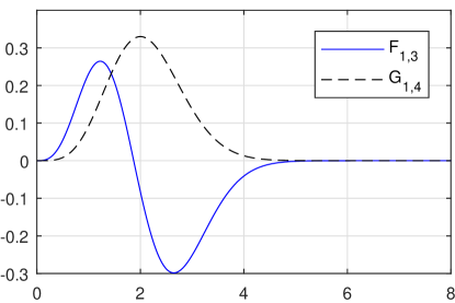
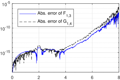
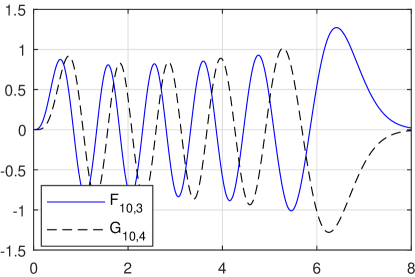
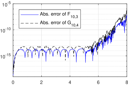
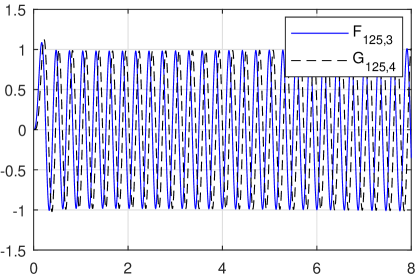
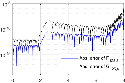
Figure 1: On the left: components $F_{n,3}$ and $G_{n,4}$ of the eigenfunction of the Dirac oscillator for $n\in\{1,10,125\}$ with the parameters $j=5/2$, $\varepsilon=-1$ and $m=\omega=1$. On the right: absolute errors of these components.

The energy spectrum can be obtained [3] from

$$E^{2}-m^{2}=m\omega\bigl{(}2(N+1)+\varepsilon(2j+1)\bigr{)}$$

for the positive-energy states, and from

$$E^{2}-m^{2}=m\omega\bigl{(}2(N+2)+\varepsilon(2j+1)\bigr{)}$$

for the negative-energy states. Here $N=2n+l$, $n=0,1,2,\ldots$, is the principal quantum number. The corresponding eigenfunctions are given by

$$F_{n,l}(r) =A\left(r\sqrt{m\omega}\right)^{l+1}\exp(-m\omega r^{2}/2)L_{n}^{l+1/2}(m\omega r^{2}),$$ (26)

$$G_{n,l-\varepsilon}(r) =A\left(r\sqrt{m\omega}\right)^{l+1-\varepsilon}\exp(-m\omega r^{2}/2)L_{n+\varepsilon/2-1/2}^{l-\varepsilon+1/2}(m\omega r^{2}),$$ (27)

where $L_{k}^{s}(x)$ is an associated Laguerre polynomial.

The system (24)–(25) is of the type considered in this paper. Since the potential of the problem is increasing, we approximated the semiaxis spectral problem (of finding the values of $E$ for which the regular solution belongs to $L_{2}(0,\infty)$) by truncating the potential and considering the Dirichlet boundary condition. For any non-trivial solution both $f_{\kappa}$ and $g_{\kappa}$ can not be equal to zero at one point, so we choose the function $f_{\kappa}$ and considered

$$f_{\kappa}(B)=0$$

as the boundary condition for the problem truncated onto $[0,B]$ segment. We refer the reader to [22, Section 7.4] for additional details on the convergence of the eigenvalues of truncated problems to the exact ones.

$\varepsilon=1$	$\varepsilon=-1$

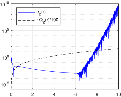
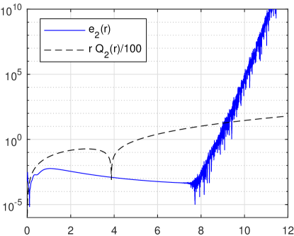
Figure 2: Application of formula (22) to determine optimal truncation interval for the Dirac oscillator with the parameters $j=5/2$ and $m=\omega=1$. On both plots black dashed line shows the value of $|rQ_{2}(r)/100|$, and the blue solid line shows $e_{2}(r):=\min_{N(r)\leq 100}\bigl{|}\sum_{n=0}^{N(r)}(-1)^{n}\beta_{2,n}(r)-rQ_{2}(r)/2\bigr{|}$ for computed coefficients $\beta_{2,n}$.

All the computations were performed in machine precision using Matlab 2017. We refer the reader to [18] for the details of the numerical realization. We considered two sets of parameters, having $\varepsilon=\pm 1$ and in both $j=5/2$ and $m=\omega=1$. For $\varepsilon=1$ the corresponding potential is $p=-m\omega r$ in the notations of (2), (3), and for $\varepsilon=-1$ the corresponding potential is $p=m\omega r$. In the first case the corresponding particular solution $f_{0}$ given by (9) is rapidly increasing, for the second case $f_{0}$ is rapidly decreasing. We decided to not implement interval subdivision techniques, and utilize the proposed representation directly to illustrate that even straightforward implementation can deliver highly accurate results.

First, we compare approximate solutions with the exact ones for the case $\varepsilon=-1$ for three eigenvalues $E^{2}-m^{2}\in\{4,40,500\}$, corresponding to $n\in\{1,10,125\}$. In terms of the system (2), (3) we have taken $\omega_{1}=2$, $\omega_{2}\in\{2,20,250\}$. On Figure 1 we present the solutions and corresponding absolute errors. As one can observe, the error does not increase for large values of $\omega$ (corresponding to higher index eigenfunctions) and only increases for large values of $r$ due to machine precision limitations. The approach presented in Remark 5 delivered a more accurate solution component $G$. This is due to the error near $r=0$ in the particular solution $g_{0}$ computed by (10). For that reason on the plots we present the absolute errors obtained with the aid of the formula from Remark 5.

Approximate solution of the spectral problem requires truncating the interval. A larger interval allows one to compute more eigenvalues and more accurately. However this leads to larger errors in all the coefficients $\beta_{j,n}$ computed, due to machine precision limitations. The equality (22) can be utilized to estimate automatically a truncation parameter $B$. We took the segment $[0,20]$, represented all the functions involved by 100001 uniformly spaced on $[0,20]$ points and computed 100 coefficients $\beta_{2,n}$. After that we checked for each $r$ the convergence of partial sums in (22) to $rQ_{2}(r)/2$. Due to machine precision limitations, the difference between $\sum_{n=0}^{N}(-1)^{n}\beta_{2,n}(r)$ and $rQ_{2}(r)/2$ reaches a plateau at some particular value of $N(r)$, meaning that the difference essentially does not decrease anymore when $N$ increases. Let $e_{2}(r):=\bigl{|}\sum_{n=0}^{N(r)}(-1)^{n}\beta_{2,n}(r)-rQ_{2}(r)/2\bigr{|}$. We chose as the truncation parameter $B$ the value $0.99\cdot r_{0}$, where $r_{0}$ is such that for all $r<r_{0}$ the value $e_{2}(r)$ is small in comparison with $rQ_{2}(r)$ (to be more precise, $e_{2}(r)<|rQ_{2}(r)|/100$), but for $r>r_{0}$ the error $e_{2}(r)$ can be larger than $|rQ_{2}(r)|/100$. As a result, $B=7.4786$ was chosen for $\varepsilon=1$, and $B=9.0168$ was chosen for $\varepsilon=-1$. See Figure 2 illustrating this procedure.

In Table 1 we present approximate eigenvalues $E^{2}-m^{2}$ for the parameters $\varepsilon=\pm 1$, $j=5/2$, $m=\omega=1$ computed on the truncated intervals $[0,B]$.

$\varepsilon=1$, on $[0,7.4786]$	$\varepsilon=-1$, on $[0,9.0168]$
Exact $E^{2}-m^{2}$ Approximate 14 13.999999999987 18 17.9999999998183 22 21.9999999982828 26 25.9999999642871 30 29.9999994276682 34 33.9999942694057 38 37.9999616653564 42 42.0001005681044 46 46.000048366715 50 50.0125330275323 54 54.0378367431326 58 58.2112436119225 Number of $\beta_{2,n}$ used 24	Exact $E^{2}-m^{2}$ Approximate 0 $7.8\cdot 10^{-32}$ 4 3.99999999999999 8 7.99999999999994 12 12.0000000000002 16 16.0000000000035 20 20.0000000000206 24 24.0000000000766 28 27.9999999997443 32 32.0000000015208 36 35.9999999944383 40 39.9999997918537 44 44.0000015951936 48 48.0000051599966 Number of $\beta_{2,n}$ used 29

Table 1: The eigenvalues for the Dirac oscillator problem (24), (25) truncated onto the segment $[0,B]$. Parameters used: $\varepsilon=\pm 1$, $j=5/2$, $m=\omega=1$. The last line shows the number of terms used in approximate solution (18).

References

• [1] A. D. Alhaidari, Solution of the Dirac equation for potential interaction, Int. J. Mod. Phys. A 18 (2003), No. 27, 4955–4973.
• [2] A. Baricz, D. Jankov, T. K. Pogány, Series of Bessel and Kummer-type functions. Lecture Notes in Mathematics, 2207. Springer, Cham, 2017.
• [3] J. Benítez, R. P. Martínez y Romero, H. N. Núñez-Yépez and A. L. Salas-Brito, Solution and hidden supersymmetry of a Dirac oscillator, Phys. Rev. Lett. 64 (1990), no. 14, 1643–1645.
• [4] B. B. Delgado, K. V. Khmelnytskaya and V. V. Kravchenko, The transmutation operator method for efficient solution of the inverse Sturm-Liouville problem on a half-line, Math. Meth. Appl. Sci. 42 (2019), 7359–7366.
• [5] F. Domínguez-Adame and M. A. González, Solvable linear potentials in the Dirac equation, Europhys. Lett. 13 (1990), no. 3, 193–198.
• [6] M. Eshghi and H. Mehraban, Eigen spectra in the Dirac-hyperbolic problem with tensor coupling, Chin. J. Phys. 50 (2012), No. 4, 533–543.
• [7] A. N. Ikot, H. Hassanabadi, E. Maghsoodi and V. Zarrinkamar, Approximate solutions of Dirac equation for Tietz and general Manning-Rosen potentials using SUSYQM, Letters to Elementary Particles and Atomic Nuclei, 11 (2014), No. 4(188), 673–687.
• [8] R. Jackiw and S.-Y. Pi, Persistence of zero modes in a gauged Dirac model for bilayer graphene, Phys. Rev. B, 78 (2008), 132104, 3pp.
• [9] A. N. Karapetyants, K. V. Khmelnytskaya and V. V. Kravchenko, A practical method for solving the inverse quantum scattering problem on a half line, J. Phys.: Conf. Ser. 1540 (2020), 012007, 7pp.
• [10] K. V. Khmelnytskaya and H. C. Rosu, An amplitude-phase (Ermakov–Lewis) approach for the Jackiw–Pi model of bilayer graphene, J. Phys. A: Math. Theor. 42 (2009) 042004 (11pp).
• [11] V. V. Kravchenko, On a method for solving the inverse Sturm–Liouville problem, J. Inverse Ill-pose P. 27 (2019), 401–407.
• [12] V. V. Kravchenko, Direct and inverse Sturm-Liouville problems: A method of solution, Birkhäuser, Cham, 2020.
• [13] V. V. Kravchenko, L. J. Navarro and S. M. Torba, Representation of solutions to the one-dimensional Schrödinger equation in terms of Neumann series of Bessel functions, Appl. Math. Comput. 314 (2017), 173–192.
• [14] V. V. Kravchenko, E. L. Shishkina and S. M. Torba, On a series representation for integral kernels of transmutation operators for perturbed Bessel equations, Math. Notes 104 (2018), 552–570.
• [15] V. V. Kravchenko, E. L. Shishkina and S. M. Torba, A transmutation operator method for solving the inverse quantum scattering problem. Submitted. Available at arXiv:2007.13039.
• [16] V. V. Kravchenko and S. M. Torba, A Neumann series of Bessel functions representation for solutions of Sturm-Liouville equations, Calcolo 55 (2018), article 11, 23pp.
• [17] V. V. Kravchenko and S. M. Torba, An improved Neumann series of Bessel functions representation for solutions of perturbed Bessel equations. Submitted. Available at arXiv:2005.10403v3.
• [18] V. V. Kravchenko, S. M. Torba and R. Castillo-Pérez, A Neumann series of Bessel functions representation for solutions of perturbed Bessel equations, Appl. Anal. 97 (2018), 677–704.
• [19] S. Linnaeus, Phase-integral solution of the radial Dirac equation, J. Math. Phys. 51 (2010), 032304, 13pp.
• [20] R. Lisboa, M. Malheiro, A. S. de Castro, P. Alberto and M. Fiolhais, Pseudospin symmetry and the relativistic harmonic oscillator, Phys. Rev. C, 69 (2004) 024319, 19pp .
• [21] M. Moshinsky and A. Szczepaniak, The Dirac oscillator, J. Phys. A: Math. Gen. 22 (1989) L817–L819.
• [22] J. D. Pryce, Numerical solution of Sturm-Liouville problems, Oxford: Clarendon Press, 1993.
• [23] G. N. Watson, A Treatise on the theory of Bessel functions, 2nd ed., reprinted, Cambridge University Press, Cambridge, UK, 1996, vi+804 pp.
• [24] J. E. Wilkins, Neumann series of Bessel functions, Trans. Amer. Math. Soc. 64 (1948), 359–385.