The Phase of the BAO on Observable Scales

Daniel Green and Alexander K. Ridgway

Department of Physics, University of California at San Diego, La Jolla, CA 92093, USA

Abstract

The baryon acoustic oscillations (BAO) provide an important bridge between the early universe and the expansion history at late times. While the BAO has primarily been used as a standard ruler, it also encodes recombination era physics, as demonstrated by a recent measurement of the neutrino-induced phase shift in the BAO feature. In principle, these measurements offer a novel window into physics at the time of baryon decoupling. However, our analytic understanding of the BAO feature is limited, particularly for the range of Fourier modes measured in surveys. As a result, it is unclear what the BAO phase teaches us about the early universe beyond what is already known from the cosmic microwave background (CMB). In this paper, we provide a more complete (semi-)analytic treatment of the BAO on observationally relevant scales. In particular, we compute corrections to the frequency and phase of the BAO feature that arise from higher order effects which occur in the tight coupling regime and during baryon decoupling. The total phase shift we find is comparable to a few percent shift in the BAO scale (frequency) and thus relevant in current data. Our results include an improved analytic calculation of the neutrino induced phase shift template that is in close agreement with the numerically determined template used in measurements of the CMB and BAO.

1 Introduction

Measurements of the Baryon Acoustic Oscillations (BAO) [1, 2] play an essential role in our understanding of the universe, connecting the physics of recombination [1] and the expansion history at low redshift [3]. While the signal-to-noise of the measurement of the BAO [4, 5, 6] is much weaker than that of the cosmic microwave background (CMB) [7], it is an invaluable tool for understanding the expansion history and breaking degeneracies. For example, a future cosmological measurement of the sum of neutrino masses requires a DESI [8] or Euclid [9] level BAO measurement of $\omega_{m}$ to accurately determine the amplitude of clustering [10, 11, 12]. Furthermore, with their ever-expanding size and depth, galaxy surveys are increasingly able to make competitive measurements without input from the CMB (see e.g. [13, 14, 15, 16, 17]).

Despite the importance of the BAO to observational cosmology, our analytic understanding of the linear BAO remains significantly less-developed than the CMB [18]. Instead, the majority of theoretical work has been focused on important non-linear effects that uniquely impact the BAO measurements, such as nonlinear damping [19, 20, 21, 22, 23] and reconstruction [24, 25, 26, 27, 28, 29]. Nevertheless, measurements are at the point where additional BAO phase information can be measured [14]. Furthermore, the BAO peak location is degenerate with this phase information and could potentially bias the measurement of the expansion history [30, 31]. This interplay between the BAO peak location and the phase is particularly interesting in light of the current tension in measurements of $H_{0}$ [32, 33].

The impact of cosmic neutrinos, and other light relics, presents a particularly compelling motivation to better understand corrections to the structure of acoustic peaks in the BAO [34]. These particles travel faster than sound waves in the primordial plasma and source perturbations ahead of the acoustic horizon [35, 36]. On small scales, this effect appears as a constant shift in the phase of the acoustic peaks in the CMB and the BAO. Furthermore, this shift is robust to non-linear evolution [37] (like the BAO peak itself [38]). Combining these insights, a first measurement of cosmic neutrinos was made in [14] using data from BOSS DR12 [39]. Yet, as with the CMB [40], there are important scale dependent corrections to the observed structure of the BAO in addition to the neutrino induced phase shift. For example, it is well-known that the velocity overshoot [41, 42] associated with the decoupling of photons and baryons implies a $\frac{\pi}{2}$ shift in phase between a Fourier mode describing a temperature fluctuations in the CMB and the corresponding BAO mode. It is therefore natural to consider what additional contributions to this relative phase exist and what the measurement of the BAO could tell us about physics at the time of baryon decoupling.

Mirroring the description of the CMB, a simple qualitative description of the BAO can be described in terms of instantaneous decoupling of baryons and photons, and gives rise to an oscillatory contribution to the matter power spectrum [43],

$$\frac{\delta P(k)}{P(k)}\approx A_{\rm BAO}\,c_{s}k\,\sin\left(kr_{\rm drift}\right)\ ,$$ (1.1)

where $r_{\rm drift}$ is the sound horizon at the time of baryon decoupling and $A_{\rm BAO}$ is a constant. The appearance of a sine (rather than a cosine) is a result of the velocity overshoot described above. In this paper, we would like to understand the leading corrections to the phase of this oscillation on observables scales. These can be described schematically as

$$\frac{\delta P(k)}{P(k)}\approx{\cal A}_{\rm BAO}\,c_{s}k\,\sin\left(kr_{\rm drift}+\sum_{i}\varphi_{i}(k)\right)\ ,$$ (1.2)

where each $\varphi_{i}(k)$ is a correction to the phase at leading order in some small parameter. The CMB analogue of this calculation was performed in [40] where they determined the contributions to the CMB peak locations in $\Lambda$CDM needed to match current observations.

Some of these phase corrections will be common to both the CMB and BAO. These include the gravitational effects of matter and neutrinos prior to decoupling, as well as subleading corrections in the tight-coupling expansion. These corrections change the photon distribution prior to recombination and thus directly impact the locations of acoustic peaks of the CMB and BAO. In addition, the BAO phase is uniquely affected by baryon decoupling in a way that is distinct from the CMB. We find four such contributions that correct the BAO phase, resulting from the photon evolution during the decoupling era and its impact on the baryon (and eventually matter) overdensity. We will see that these contributions are comparable in size to the neutrino phase shift or, alternatively, a few percent shift in the BAO scale $r_{\rm drift}$. Current measurements are sensitive to sub-percent changes to the BAO scale [4, 5, 6], and the neutrino induced phase alone [14], and thus should be sensitive to these additional phase shifts as well.

The broader motivation for this work is to understand how physics beyond $\Lambda$CDM might be uniquely encoded in the BAO. However, such an exploration is challenging without first having a complete understanding of the phase in $\Lambda$CDM. This is particularly pertinent to the BAO, in contrast to the CMB, since the data is typically reduced to a standard ruler which does not directly contain the phase information. While this is valid in many models [31], the (semi)-analytic description of the BAO we describe in this paper should make a systematic exploration of the effects of new physics on the BAO phase more tractable.

The paper is organized as follows: In section 2, we review the equations of the linear evolution and the conventional derivation of the BAO signal. In section 3, we determine phase corrections associated with the tight coupling regime, including the effect of free-streaming neutrinos. In section 4, we calculate the impact of physics at the time of baryon decoupling. We combine these results in section 5, where we present our full description of the BAO phase and conclude in section 6. A few technical details of these calculations are relegated to appendices.

2 Linear Theory of the BAO

The BAO feature in the matter power spectrum can be determined by solving the linear cosmological equations [44]. In this section, we give a simplified baseline treatment of the BAO which we later improve upon in sections 3 and 4. We use Dodelson’s [45] conventions for the cosmological fluctuations throughout.

2.1 Evolution Equations and Conventions

In this section, we enumerate the equations used to derive the BAO feature in the matter power spectrum. We are interested in the evolution of the photons, baryons, dark matter and neutrinos which carry background energy densities $\bar{\rho}_{\gamma}$, $\bar{\rho}_{\rm b}$, $\bar{\rho}_{\rm dm}$, and $\bar{\rho}_{\nu}$. The metric can be expressed in conformal Newtonian gauge as

$$ds^{2}=a(\eta)^{2}\left(-(1+2\Psi({\vec{x}},\eta))d\eta^{2}+(1+2\Phi({\vec{x}},\eta))d{\vec{x}}^{2}\right)$$ (2.1)

where $a$ is the scale factor, $\Psi$ and $\Phi$ are the gravitational potentials, and $\eta$ is conformal time. The fluctuations in baryons and dark matter are characterized by their overdensities $\delta_{\rm b}({\vec{x}},\eta)=\rho_{\rm b}({\vec{x}},\eta)/\bar{\rho}_{\rm b}(\eta)$ and $\delta({\vec{x}},\eta)=\rho_{\rm dm}({\vec{x}},\eta)/\bar{\rho}_{\rm dm}(\eta)$, and velocity potentials $\tilde{v}_{\rm b}$ and $\tilde{v}$.

The photon fluctuations are described by their temperature perturbation,

$$f_{\gamma}(\vec{x},p,\hat{p},\eta)=\left[{\rm exp}\left(\frac{p}{T(\eta)(1+\Theta(\vec{x},\hat{p},\eta))}\right)-1\right]^{-1},$$ (2.2)

where $f_{\gamma}$ is the photon distribution function and $\Theta(\vec{x},\hat{p},\eta)$ represents the photon temperature fluctuation as a function of position, direction and time. The neutrino temperature perturbation $\mathcal{N}(\vec{x},\hat{p},\eta)$ is defined similarly. The temperature perturbations can be decomposed into multipole moments using a Legendre polynomial expansion:

$$\Theta_{l}\equiv\frac{1}{(-i)^{l}}\int_{-1}^{1}\frac{d\mu}{2}\mathcal{P}_{l}(\mu)\Theta(\mu)\rightarrow\Theta(\mu)=\sum_{l=0}^{\infty}(-i)^{l}(2l+1)P_{l}(\mu)\Theta_{l}$$ (2.3)

and similarly for the neutrinos.

It is useful to express the equations of motion of the metric perturbations and cosmological components in momentum space. Defining $\mu\equiv\hat{p}\cdot\hat{k}$, the relationship between the position and momentum space variables is given by

$$\Theta(\vec{x},\hat{p},\eta)=\int\frac{d^{3}k}{(2\pi)^{3}}e^{i\vec{k}\cdot\vec{x}}\Theta(\vec{k},\mu,\eta)$$ (2.4)

and similarly for the other components. We are primarily interested in wave-numbers belonging to the observable BAO range which satisfy $0.1h{\rm Mpc}^{-1}\leq k\leq 0.3h{\rm Mpc}^{-1}$, where $k\equiv|\vec{k}|$.

The time evolution of the gravitational potentials is sourced by the first three moments of the photon and neutrino temperature perturbations, as well as by the baryon and dark matter overdensities and velocities. Defining $v\equiv i\tilde{v}$ and $v_{b}\equiv i\tilde{v}_{b}$, the linear Einstein’s equations are

$$\dot{a}=H_{0}\sqrt{\Omega_{r}+\Omega_{m}a}$$ (2.5)

$$k^{2}\Phi=4\pi Ga^{2}(\bar{\rho}_{m}\delta_{m}+4\bar{\rho}_{r}\Theta_{r,0}+\frac{3aH}{k}(\bar{\rho}_{m}v_{m}+4\bar{\rho}_{r}\Theta_{r,1}))$$ (2.6)

$$k^{2}\left(\Phi+\Psi\right)=-32\pi Ga^{2}\bar{\rho}_{r}\Theta_{r,2}$$ (2.7)

where overhead dots represent derivatives with respect to $\eta$. Note, the linear combinations of the matter and radiation perturbations that source the gravitational potentials are $\bar{\rho}_{m}\delta_{m}\equiv\bar{\rho}_{\rm dm}\delta+\bar{\rho}_{b}\delta_{b}$, $\bar{\rho}_{m}v_{m}\equiv\bar{\rho}_{\rm dm}v+\bar{\rho}_{b}v_{b}$, and $\bar{\rho}_{r}\Theta_{r}\equiv\bar{\rho}_{\gamma}\Theta+\bar{\rho}_{\nu}\mathcal{N}$. We have also defined $\Omega_{i}\equiv\bar{\rho}_{i}/\rho_{cr}$, where $\rho_{cr}$ denotes the critical energy density. With the exception of section 3.2, we set $\Theta_{r,2}=0$ and freely make use of $\Phi=-\Psi$.

The dark matter only interacts gravitationally with the other components:

$$\dot{\delta}+kv=-3\dot{\Phi},\ \dot{v}+\frac{\dot{a}}{a}v=k\Psi.$$ (2.8)

Baryons, on the other hand, experience gravitational and electromagnetic interactions with the other components. Mass conservation implies

$$\dot{\delta}_{b}+kv_{b}=-3\dot{\Phi}$$ (2.9)

and conservation of momentum yields

(2.10)

where we have defined

$$\dot{\tau}=-\bar{n}_{e}\sigma_{\rm T}a,\ R=\frac{3\bar{\rho}_{b}}{4\bar{\rho}_{\gamma}}.$$ (2.11)

to parameterize the Thompson scattering of photons off free electrons. In equation (2.11), $\sigma_{T}$ is the Thompson scattering cross section and $\bar{n}_{e}$ is the background free electron number density.

The equations describing the time evolution of the full photon and neutrino temperature perturbations are

$$\dot{\Theta}+ik\mu\Theta =-\dot{\Phi}-ik\mu\Psi-\dot{\tau}(\Theta_{0}-\Theta-i\mu v_{b}-\frac{1}{2}P_{2}(\mu)\Pi)$$ (2.12)

$$\dot{\mathcal{N}}+ik\mu\mathcal{N} =-\dot{\Phi}-ik\mu\Psi.$$

where $\Pi\equiv\Theta_{2}+\Theta^{P}_{0}+\Theta^{P}_{2}$ and $\Theta^{P}$ denotes the temperature perturbation for photon polarizations. Outside of section 3.3, which considers the effects of diffusion damping, we set $\Pi=0$. Using (2.3), (2.12) can be broken into equations describing the first few multipole moments:

$$\ \ \ \ \ \ \ \dot{\mathcal{N}}_{0}+k\mathcal{N}_{1}=-\dot{\Phi},\ \dot{\mathcal{N}}_{1}-\frac{k}{3}(\mathcal{N}_{0}-2\mathcal{N}_{2})=\frac{k}{3}\Psi$$ (2.13)

$$\dot{\Theta}_{0}+k\Theta_{1}=-\dot{\Phi},\ \dot{\Theta}_{1}-\frac{k}{3}(\Theta_{0}-2\Theta_{2})=\frac{k}{3}\Psi+\frac{\dot{\tau}}{3}(3\Theta_{1}-v_{b}).$$ (2.14)

It is often convenient to use the $k\Theta_{1}=-\dot{\Theta}_{0}-\dot{\Phi}$ in the dipole equation to get

(2.15)

The LHS takes the form of a wave-equation, as expected. Outside of sections 3.3 and 4.2, where we consider corrections to the tight coupling approximation and free-streaming effects near decoupling, we set $\Theta_{2}=0$. In the tight coupling regime, it is useful to eliminate $v_{b}$ using (2.10).

In this paper, the initial conditions of the cosmological variables are expressed in units of the primordial adiabatic fluctuation $\zeta\equiv\Phi-ik_{i}\delta T^{0}_{i}H/(k^{2}(\rho+P))$ as $\tau\to 0$. Since we are interested in the linear impact of baryons on the matter transfer function, which is independent of the statistics of the primordial fluctuations, we are free to set $\zeta=1$ throughout.

2.2 Baseline Derivation of the BAO

We begin by giving a simplified derivation of the BAO feature in the matter overdensity, following [43]. From the start of radiation domination to the era of decoupling, the baryons and photons are tightly coupled and oscillate in phase with each other, i.e. $v_{b}=3\Theta_{1}+O(k/\dot{\tau})$. The pressure from photon scatterings prevents the gravitational collapse of baryons and the amplitude of the baryon perturbation is comparable to that of the photons. Over time, the expansion of the universe causes the photon-baryon scattering rate to decrease. The baryons eventually decouple from the photons and undergo gravitational collapse. The oscillation frequency of the photon-baryon system depends on the wavenumber $k$, meaning different baryon modes decouple at different phases in their oscillations. The initial conditions for the gravitational growth of the baryons then have an oscillatory shape which gives rise to the BAO.

It is useful to work backwards and first consider the evolution of the baryons after they decouple from the photons. Combining Poisson’s equation (2.6) with the evolution equations for the dark matter (2.8) and baryons (2.10) gives a closed set of equations describing the full matter perturbation:

$$\dot{\delta}_{m}+kv_{m}=0,\ \dot{v}_{m}+\frac{\dot{a}}{a}v_{m}=-k\Phi,\ k^{2}\Phi=\frac{3H_{0}^{2}}{2a}\Omega_{m}\delta_{m}.$$ (2.16)

Since $k\gg aH$ near decoupling, $\delta_{m}$ is well approximated by the large $k$ solutions first obtained by Meszaros [46],

$$\delta_{m}(k,y)=C_{1}(k)D_{1}(y)+C_{2}(k)D_{2}(y)$$ (2.17)

where

$$D_{1}(y)=y+2/3,\ D_{2}(y)=D_{1}(y){\rm ln}\left(\frac{\sqrt{1+y}+1}{\sqrt{1+y}-1}\right)-2\sqrt{1+y},\ y=a/a_{\rm eq}.$$ (2.18)

In the limit of late times, the growing solution $D_{1}$ scales as $D_{1}(y)\sim y$ while the decaying one $D_{2}$ scales as $D_{2}(y)\sim 1/y^{3/2}$. Therefore, the resulting matter overdensity at low-redshift is given by $\delta_{m}(k,y)\simeq C_{1}(k)D_{1}(y)$.

Poisson’s equation in (2.16) implies that once the growing mode dominates, the position dependence of the gravitational potential is proportional to the Fourier transform of $C_{1}(k)/k^{2}$. This encodes the location of the gravitational potential wells that both dark matter and baryons fall into and eventually reside in at late times. The $C_{i}(k)$ depend on the initial locations of the dark matter and baryons as they begin to undergo gravitational growth. They are fixed by matching $\delta_{m}$ and its derivative to the expression for $\delta_{m}$ valid before the baryons fully decouple from the photons. The matching conditions are

$$C_{1}(k)D_{1}(y(\eta_{g}))+C_{2}(k)D_{2}(y(\eta_{g}))=\frac{\Omega_{b}}{\Omega_{m}}\delta_{b}(\eta_{g})+\frac{\Omega_{\rm cdm}}{\Omega_{m}}\delta(\eta_{g}),$$ (2.19)

$$C_{1}(k)\dot{D}_{1}(y(\eta_{g}))+C_{2}(k)\dot{D}_{2}(y(\eta_{g}))=\frac{\Omega_{b}}{\Omega_{m}}\dot{\delta}_{b}(\eta_{g})+\frac{\Omega_{\rm cdm}}{\Omega_{m}}\dot{\delta}(\eta_{g}).$$

We choose $\eta_{g}$ to be some when the gravitational force on baryons dominates over photon-baryon scatterings ($\dot{\tau}\ll k\Phi$) and the dark matter overdensity is still the largest source of gravity ($\delta\gg\delta_{b}$). The growing mode coefficient can be split into terms coming from the dark matter and baryons, $C_{1}\equiv C_{\rm cdm}+C_{\rm BAO}$. Focusing on the baryonic piece, the matching condition gives

$$C_{\rm BAO}(k) =\frac{\Omega_{b}}{\Omega_{m}}\frac{D_{2}}{D_{1}\dot{D}_{2}-D_{2}\dot{D}_{1}}(kv_{b}+\frac{\dot{D}_{2}}{D_{2}}\delta_{b})\simeq-\frac{2k}{5\dot{y}}\frac{\Omega_{b}}{\Omega_{m}}(v_{b}-\frac{3aH}{2k}\delta_{b})$$ (2.20)

where all functions of time in (2.20) are evaluated at $\eta_{g}$. In the last equality, we approximated $y(\eta_{g})\gg 1$ and replaced the $D_{i}$ with their asymptotic expressions.

Since $k\gg aH(\eta_{g})$, the term proportional to $\delta_{b}$ can be neglected, giving

$$C_{\rm BAO}(k)\simeq-\frac{2k}{5\dot{y}(\eta_{g})}\frac{\Omega_{b}}{\Omega_{m}}v_{b}(k,\eta_{g}).$$ (2.21)

The leading behavior of the BAO profile is then given by the scale dependence of $v_{b}(k,\eta_{g})$. The fact that the BAO is fixed by the scale dependence of $v_{b}$ and not $\delta_{b}$ is the well known “velocity overshoot” effect [41, 42]. Equations (2.17) and (2.21) then give the BAO feature in the total matter overdensity.

To determine $v_{b}(k,\eta_{g})$ and evaluate (2.21), one simply integrates (2.10):

$$v_{b}(k,\eta_{g})=-\frac{3}{a(\eta_{g})}\int_{-\infty}^{\eta_{g}}d\eta a(\eta)g_{b}(\eta)\Theta_{1}(k,\eta)+I_{\Phi}(k,\eta_{g}).$$ (2.22)

We have defined the baryon visibility function [43] $g_{b}(\eta)$ through

$$\tau_{b}(\eta)\equiv\int^{\eta}d\eta^{\prime}\frac{\dot{\tau}}{R},\ g_{b}\equiv\dot{\tau}_{b}e^{-\tau_{b}}$$ (2.23)

and written the contribution from gravity as

$$I_{\Phi}(k,\eta)\equiv-\frac{k}{a(\eta)}\int_{-\infty}^{\eta}d\eta^{\prime}a(\eta^{\prime})e^{\tau_{b}(\eta)-\tau_{b}(\eta^{\prime})}\Phi(\eta^{\prime}).$$ (2.24)

The first term in (2.22) gives the cumulative effect of the photon driving force on $v_{b}$ and is responsible for the oscillatory shape of the BAO. The contribution from $I_{\Phi}$ has no oscillatory information and only shifts the average value of the BAO feature.

The evolution of the tightly coupled photons can be obtained by using (2.10) to eliminate $(3\Theta_{1}-v_{b})$ from (2.15), yielding

$$(\partial_{\eta}^{2}+k^{2}c_{s}^{2})(\Theta_{0}+\Phi)=\frac{k^{2}}{3}(1+\frac{1}{1+R})\Phi,$$ (2.25)

where $c_{s}=1/\sqrt{3(1+R)}$ gives the speed of sound of the photon-baryon fluid. In deriving (2.25), we have only kept leading order terms in $k/\dot{\tau}$ (e.g. $v_{b}=3\Theta_{1}+{\cal O}(k/\dot{\tau})$) and dropped the drag term proportional to $\dot{a}/a$. Near decoupling, the gravitational source in (2.25) is negligible and the photon perturbations are given by

$$\Theta_{0}(k,\eta)+\Phi(k,\eta) \simeq-{\rm cos}(kr_{s}(\eta))\implies\Theta_{1}(k,\eta)\simeq-c_{s}(\eta){\rm sin}(kr_{s}(\eta))$$ (2.26)

where $r_{s}(\eta)=\int^{\eta}d\eta^{\prime}c_{s}(\eta^{\prime})$ is the sound horizon of the photon-baryon fluid. The minus signs in (2.26) are due to the evolution of the photon perturbation during radiation domination (see Appendix A for details). In (2.26), we have only kept the leading contribution from this effect.

Equation (2.25) is the leading expression for $\Theta_{1}$ near decoupling and can be combined with (2.22) to obtain $v_{b}(k,\eta_{g})$. The baryon visibility function $g_{b}(\eta)$ represents the probability for an individual baryon to last scatter with the photons at $\eta$ and can be approximated as a Gaussian:

$$g_{b}(\eta)\simeq-\frac{1}{\sigma\sqrt{\pi}}e^{-\frac{(\eta-\eta_{*})^{2}}{\sigma^{2}}}.$$ (2.27)

Since $\eta_{g}$ is chosen after the baryons have fully decoupled from the photons, i.e. $g_{b}(\eta_{g})\simeq 0$, we can take the upper bound of the integral in (2.22) to infinity. Using the fact that (2.27) is peaked at $\eta_{*}$, the integrand can be simplified by setting $kr_{s}(\eta)\simeq kr_{s}(\eta_{*})+kc_{s}(\eta_{*})(\eta-\eta_{*})$ and $a(\eta)\simeq a(\eta_{*})$.

Evaluating (2.22) with these approximations gives our leading expression for the BAO profile

$$C_{\rm BAO}(k)=-\frac{2k}{5\dot{y}(\eta_{g})}\frac{\Omega_{b}}{\Omega_{m}}\left[-\mathcal{A}(k){\rm sin}(kr_{s}(\eta_{*}))+I_{\Phi}(k,\eta_{g})\right]$$ (2.28)

where the amplitude is given by

$$\mathcal{A}(k)\equiv 3\frac{a(\eta_{*})}{a(\eta_{g})}c_{s}(\eta_{*})e^{-\left(\frac{kc_{s}(\eta_{*})\sigma}{2}\right)^{2}}.$$ (2.29)

As already mentioned, the appearance of the sine in (2.28) is a consequence of the velocity overshoot effect, and the fact that the baryon velocity is determined by the photon dipole (2.21). The exponential in (2.29) suppresses modes that oscillate rapidly within the support of $g_{b}$, i.e. $kc_{s}(\eta_{*})\gg 1/\sigma$.

In deriving (2.28), we neglected several important effects that change the evolution of the tightly coupled photons. In addition, the treatment of the photon-baryon dynamics near decoupling was greatly simplified. Corrections to the tightly coupled photons and the physics near decoupling impact the BAO profile and are considered in sections 3 and 4.

3 Corrections to Tightly Coupled Photons

The expression for the tightly coupled photons in (2.26) neglects gravitational driving during matter domination, the gravitational influence of neutrino anisotropic stresses and higher order corrections to the tight coupling approximation. The contributions from these effects change the phase and amplitude of $\Theta_{1}$ and the driving force the photons exert on the baryons. In this section, we compute the leading corrections from each of these effects on the photon evolution. We first treat the effects separately and then combine terms in section 3.4.

3.1 Gravity Driving During Matter Domination

In deriving our original expression for the photons (2.26) during matter domination, we neglected the gravitational source on the right hand side of (2.25) and only kept the homogeneous solution. As we will show, gravitational driving during matter domination changes the zero point of the photon oscillations and shifts their phase and amplitude.

The leading contribution from gravity driving during matter domination is obtained by convolving the right hand side of (2.25) with the Green’s function for the tightly coupled photons,

$$G_{\Theta}(\eta,\eta^{\prime})=-\frac{1}{c_{s}k}({\rm cos}(kr_{s}(\eta)){\rm sin}(kr_{s}(\eta^{\prime}))-{\rm cos}(kr_{s}(\eta^{\prime})){\rm sin}(kr_{s}(\eta)))\Theta(\eta-\eta^{\prime}),$$ (3.1)

from the time of matter-radiation equality $\eta_{\rm eq}$ defined through $\bar{\rho}_{r}(\eta_{\rm eq})=\bar{\rho}_{m}(\eta_{\rm eq})$, to some time $\eta$ before decoupling. We find

$$\Theta_{0}(k,\eta)+\Phi(k,\eta)=-(1-\alpha(k,\eta)){\rm cos}(kr_{s}(\eta))+\beta(k,\eta){\rm sin}(kr_{s}(\eta))$$ (3.2)

where

$$\alpha(k,\eta) =-2k\int_{r_{s}(\eta_{\rm eq})}^{r_{s}(\eta)}dx{\rm sin}(kx)\Phi(k,\sqrt{3}x)$$ (3.3)

$$\beta(k,\eta) =2k\int_{r_{s}(\eta_{\rm eq})}^{r_{s}(\eta)}dx{\rm cos}(kx)\Phi(k,\sqrt{3}x).$$

In writing (3.3), we changed integration variables to $x=r_{s}(\eta)$ and approximated $1+\frac{1}{1+R}\simeq 2$.

To evaluate (3.3), we need an expression for the gravitational potential $\Phi$ valid in the range $\eta_{\rm eq}<\eta<\eta_{*}$. During this time, the dark matter overdensity gives the largest contribution to $\Phi$ since $\delta_{b}\sim\Theta_{0}\ll\delta$. The equations describing $\delta$ and $\Phi$ are identical to (2.16) with $\delta_{m}$ and $v_{m}$ replaced with $\delta$ and $v$. One can approximate $k\gg aH$ during matter domination, which means $\delta(k,\eta)=\delta_{1}(k)D_{1}(y)+\delta_{2}(k)D_{2}(y)$. Neglecting the decaying mode $D_{2}$, the gravitational potential takes the form

$$\Phi(k,y)=\frac{3}{2k^{2}}\frac{H_{0}^{2}}{\Omega_{r}}\Omega_{m}\Omega_{\rm dm}\delta_{1}(k)(1+\frac{2}{3y})\equiv\Phi_{k}(1+\frac{2}{3y}).$$ (3.4)

The scale dependence of the gravitational potential $\Phi_{k}$ can be obtained by fitting (3.4) to the numerical solution of $\Phi$ (e.g. using matter transfer function output from a Boltzmann code like CLASS [47] or a fitting function like BBKS [48]).

The fact that the scale and time dependence of $\Phi(k,y)$ factorizes simplifies (3.3). Working in the limit $kr_{s}(\eta_{\rm eq})\gg 1$, and using $y=a(\eta)\Omega_{m}/\Omega_{r}$ and $a(\eta)=\frac{1}{4}\eta^{2}H_{0}^{2}\Omega_{m}+\eta H_{0}\sqrt{\Omega_{r}}$, we find

$$\alpha(k,\eta)={\rm cos}(kr_{s}(\eta))f_{\Phi}(k,\eta)-{\rm cos}(kr_{s}(\eta_{\rm eq}))f_{\Phi}(k,\eta_{\rm eq})$$ (3.5)

$$\beta(k,\eta)={\rm sin}(kr_{s}(\eta))f_{\Phi}(k,\eta)-{\rm sin}(kr_{s}(\eta_{\rm eq}))f_{\Phi}(k,\eta_{\rm eq})$$

$$\tilde{x}=\frac{4}{H_{0}\Omega_{m}}\sqrt{\frac{\Omega_{r}}{3}},\ f_{\Phi}(k,\eta)=2\Phi_{k}\left(1+\frac{\tilde{x}}{6}\left(\frac{1}{r_{s}(\eta)}-\frac{1}{r_{s}(\eta)+\tilde{x}}\right)\right).$$

Inserting (LABEL:phi_integration_theta0) into (3.2) gives

$$\Theta_{0}(k,\eta)+\Phi(k,\eta)=f_{\Phi}(k,\eta)-(1-A_{\Phi}(k)){\rm cos}(kr_{s}(\eta))+B_{\Phi}(k){\rm sin}(kr_{s}(\eta))$$ (3.6)

where we have defined

$$A_{\Phi}(k)=-{\rm cos}(kr_{s}(\eta_{\rm eq}))f_{\Phi}(\eta_{\rm eq}),\ B_{\Phi}=-{\rm sin}(kr_{s}(\eta_{\rm eq}))f_{\Phi}(\eta_{\rm eq})).$$ (3.7)

Equation (3.6) implies gravitational driving during matter domination shifts the zero point of the photon oscillations by $f_{\Phi}$, and induces the phase shift

$$\phi_{\Phi}\simeq{\rm sin}^{-1}(B_{\Phi}).$$ (3.8)

The phase shift is then proportional to the transfer function of the gravitational potential $\Phi_{k}$. It is well known that for modes entering the horizon before matter-radiation equality, the transfer function decreases with increasing $k$. The observable BAO modes satisfy $k>aH(\eta_{\rm eq})$, which means the BAO phase shift resulting from $\phi_{\Phi}$ is largest for modes at the lower end of the observable range.

3.2 Neutrino Anisotropic stresses

In this section, we compute the effects of neutrino anisotropic stress on the evolution of the photons. Unlike the tightly coupled photons, neutrinos free stream at nearly the speed of light in vacuum during radiation domination. This means their anisotropic stress, parametrized by $\mathcal{N}_{2}$, is not suppressed relative to $\mathcal{N}_{0}$ or $\mathcal{N}_{1}$. Since neutrinos travel faster than the speed of sound of the photon-baryon fluid, they source a unique contribution to the gravitational potential that is correlated at distances larger than $r_{s}(\eta)$. This induces a phase shift in the photon oscillations which changes the peak locations of both the CMB [35, 36] and BAO [37].

The gravitational effects of free streaming neutrinos on photons can be computed similarly to how the gravitational effects of matter were evaluated in section 3.1. The difference here is that since we are including a finite $\mathcal{N}_{2}$, the constraint equation (2.7) implies $\Phi\neq-\Psi$. The gravitational source on the right hand side of (2.25) now consists of the combination $\Phi_{-}\equiv\Phi-\Psi$. The leading contribution from neutrino anisotropic stress can be written

$$\Theta_{0}(k,\eta)+\Phi(k,\eta)=-(1-A_{\nu}(k,\eta)){\rm cos}(kr_{s}(\eta))+B_{\nu}(k,\eta){\rm sin}(kr_{s}(\eta))$$ (3.9)

$$A_{\nu}(\eta)=-kc_{s}\int_{0}^{\eta}d\eta^{\prime}{\rm sin}kr_{s}(\eta^{\prime})\Phi^{(1)}_{-}(\eta^{\prime}),\ B_{\nu}(\eta)=kc_{s}\int_{0}^{\eta}d\eta^{\prime}{\rm cos}kr_{s}(\eta^{\prime})\Phi^{(1)}_{-}(\eta^{\prime})$$

where $\Phi^{(1)}_{-}$ denotes the leading correction to $\Phi_{-}$ from the gravitational effects of $\mathcal{N}_{2}$.

According to equation (2.7), the symmetric combination $\Phi_{+}\equiv\Phi+\Psi$ is sourced by the neutrino anisotropic stress. To determine $\mathcal{N}_{2}$, it is useful to first solve (2.12) for the full neutrino temperature perturbation,

$${\mathcal{N}}(\mu,\eta)={\mathcal{N}}_{\rm in}e^{-ik\mu\eta}-\int_{0}^{\eta}d\eta^{\prime}e^{-ik\mu(\eta-\eta^{\prime})}(\dot{\Phi}+ik\mu\Psi),$$ (3.10)

and to break (3.10) into multipole moments using the plane wave expansion

$$e^{-ik\mu\eta}=\sum_{l=0}^{\infty}(-i)^{l}(2l+1)P_{l}(\mu)j_{l}(k\eta)$$ (3.11)

and (2.3) for neutrinos. Using (3.10) and (3.11) and projecting out the quadrupole component, we find

$${\mathcal{N}}_{2}(x)=({\mathcal{N}}_{\rm in}+\Phi_{\rm in})j_{2}(c_{s}^{-1}x)-c_{s}^{-1}\int_{0}^{x}dx^{\prime}j_{2}^{\prime}(c_{s}^{-1}(x-x^{\prime}))\Phi_{-}(x^{\prime}).$$ (3.12)

where $x\equiv kc_{s}\eta$.

The largest gravitational interactions between free streaming neutrinos and photons occur during radiation domination. This can be understood heuristically by considering the evolution of initial spikes in the photon-baryon fluid and neutrino distribution. Since the neutrinos travel faster than the tightly coupled photons, the distance between the neutrino spike and the photon-baryon one gets larger as time goes on and the strength of their gravitational interaction decreases. To a good approximation, the effect of free streaming neutrinos on the photons can be computed using expressions valid during radiation domination. Only a small error is accumulated by using these expressions during matter domination, because by this time the gravitational effects of free-streaming neutrinos on photons has become small.

The gravitational effect of $\mathcal{N}_{2}$ can be derived by combining (2.13) and (2.14) with (2.6) and (2.7). Using $a(\eta)\sim\eta$ and the fact that the modes of interest are well inside the horizon during radiation domination (i.e. $k\eta\gg 1$), we find

$$\Phi^{\prime\prime}_{-}+\frac{4}{x}\Phi^{\prime}_{-}+\Phi_{-}=-S(\Phi_{+}),\ S(\Phi_{+})\equiv\Phi^{\prime\prime}_{+}+\frac{2}{x}\Phi^{\prime}_{+}+3\Phi_{+},\ \Phi_{+}(x)=-\frac{4\epsilon_{\nu}}{x^{2}}{\mathcal{N}}_{2}(x).$$ (3.13)

Equation (3.13) can be computed perturbatively in $\epsilon_{\nu}$. The leading correction to $\Phi_{-}$ is given by

$$\Phi^{(1)}_{-}(x)=-\frac{4\epsilon_{\nu}}{15}\frac{{\rm sin}x-x{\rm cos}x}{x^{3}}-\int_{0}^{x}dx^{\prime}G(x,x^{\prime})S(\Phi_{+}(x^{\prime}))$$ (3.14)

$$G(x,x^{\prime})=\Theta(x-x^{\prime})\frac{x^{\prime}}{x^{3}}((x^{\prime}-x){\rm cos}(x^{\prime}-x)-(1+xx^{\prime}){\rm sin}(x^{\prime}-x)),$$

where the first term is due to the change in initial conditions from neutrino anisotropic stress (see Appendix B).

We are interested in evaluating (LABEL:fs_for_phase) at $\eta_{*}$, the peak of the baryon visibility function. It is useful to write

$$B_{\nu}(k,\eta_{*})=\int_{0}^{\infty}dx\,{\rm cos}x\,\Phi_{-}^{(1)}(x)-\int_{kr_{s}(\eta_{*})}^{\infty}dx\,{\rm cos}x\,\Phi^{(1)}_{-}(x)$$ (3.15)

and similarly for $A_{\nu}$. The first term in (3.15) is scale-independent and can be evaluated numerically, while the remaining integral is scale dependent. Since $kr_{s}(\eta_{*})\gg 1$, the second integral can be computed perturbatively in $1/kr_{s}(\eta_{*})$.

In the limit $x\rightarrow\infty$, the source function $S(\Phi_{+}(x))$ in (LABEL:potentials_m) decays to zero. This can be seen directly from the expression for $\mathcal{N}_{2}$ in (3.12) since the factors of spherical Bessel functions and $\Phi_{-}$ vanish in this limit. The physical reason the source vanishes is because the spatial separation between the free streaming neutrinos and sound horizon gets large as $x\rightarrow\infty$ and, as a result, the gravitational source function decays to zero.

Since $S(x)\rightarrow 0$ in the limit of large $x$, the $x^{\prime}$ integral in (LABEL:potentials_m) can be approximated by extending the upper bound from $x$ to $\infty$. The dependence on $x$ and $x^{\prime}$ then factorizes and the integrations over $x^{\prime}$ can be performed numerically. The $O(\epsilon_{\nu})$ integrand can be obtained by first plugging the zeroth order solution of $\Phi_{-}$ (i.e. the homogeneous solution of (3.13)) into (3.12) to find the zeroth order expression for $\mathcal{N}_{2}$. Combining the result with (3.13) then gives $S(\Phi_{+})$ to $O(\epsilon_{\nu})$. After performing the $x^{\prime}$ integrals numerically, equation (LABEL:potentials_m) yields

$$\Phi^{(1)}_{-}(x\gg 1)\simeq-\frac{4\epsilon_{\nu}}{15}\frac{{\rm sin}x-x{\rm cos}x}{x^{3}}+\frac{{\rm cos}x}{x^{3}}(\kappa_{1}-x\kappa_{2})+\frac{{\rm sin}x}{x^{3}}(\kappa_{2}+x\kappa_{1})$$ (3.16)

where

$$\kappa_{1} \equiv-\int_{0}^{\infty}dx^{\prime}(x^{\prime 2}{\rm cos}x^{\prime}-x^{\prime}{\rm sin}x^{\prime})S(x^{\prime})\simeq 2.3\epsilon_{\nu}$$ (3.17)

$$\kappa_{2} \equiv-\int_{0}^{\infty}dx^{\prime}(x^{\prime 2}{\rm sin}x^{\prime}+x^{\prime}{\rm cos}x^{\prime})S(x^{\prime})\simeq-4.8\epsilon_{\nu}.$$

The scale dependent integral in (3.15) can be computed analytically using (3.16). The gravitational influence of neutrino anisotropic stress is then given by

$$A_{\nu}(k,\eta_{*})=0.44\epsilon_{\nu}+\frac{\kappa_{1}}{2kr_{s}}+\frac{15\kappa_{1}{\rm sin}2kr_{s}+(15\kappa_{2}-4\epsilon_{\nu})(1-{\rm cos}2kr_{s})}{60(kr_{s})^{2}}$$ (3.18)

$$B_{\nu}(k,\eta_{*})=0.58\epsilon_{\nu}+\frac{1}{kr_{s}}(\frac{\kappa_{2}}{2}-\frac{2\epsilon_{\nu}}{15})-\frac{15\kappa_{1}(1+{\rm cos}2kr_{s})+(15\kappa_{2}-4\epsilon_{\nu}){\rm sin}2kr_{s}}{60(kr_{s})^{2}}$$

where all factors of $r_{s}$ in (LABEL:f_nus_pieces) are evaluated at $\eta_{*}$.

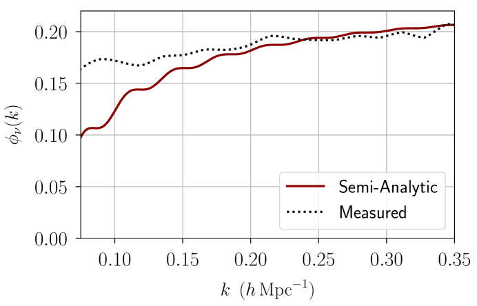
Figure 1: Phase shift due to neutrino anisotropic stresses. The solid curve is the semi-analytic model of the phase shift obtained in (3.19). The dotted line is the phase shift measured in [30] using the output of CLASS for different values of $N_{\rm eff}$, holding the frequency and matter-radiation equality fixed. The measured value does not uniquely isolate the contribution from anisotropic stress and thus it is possible the mild disagreement at low-$k$ is simply a difference in how $\phi_{\nu}(k)$ is defined in each case.

Equations (LABEL:fs_for_phase) and (LABEL:f_nus_pieces) imply the phase shift of $\Theta_{0}$ due to neutrino anisotropic stresses is

$$\phi_{\nu}(k)={\rm sin}^{-1}(B_{\nu}(k,\eta_{*})).$$ (3.19)

As $k\rightarrow\infty$, the phase shift approaches a constant [35, 36]. The leading scale dependence is given by the simple power law $1/(kr_{s})$, while the $1/(kr_{s})^{2}$ correction adds an oscillatory profile on top of the leading behavior. This is depicted in Figure 1, which plots (3.19) against a numerical evaluation of $\phi_{\nu}$ [30]. The figure suggests that the BAO phase shift due to neutrino anisotropic is nearly constant for $k\sim 0.3h{\rm Mpc}^{-1}$.

3.3 Higher-Order in Tight Coupling

Up to this point we have worked to leading order in the tight coupling approximation. Terms higher order in $k/\dot{\tau}$ represent the fact that individual photons travel a finite distance between scatterings and undergo a random walk [49, 43]. The photon diffusion length is given by the average distance of the random walk and sets the scale below which correlations in the photon temperature perturbation are washed out. Perturbations at distance scales below the diffusion length are suppressed and, as a result, the BAO amplitude is smaller at these scales.

Higher order terms in the tight coupling approximation then contribute damping terms to (2.25). The change in the photon oscillations is analogous to what happens when a damping force is added to a harmonic oscillator. In particular, the amplitude decreases and the phase gets shifted for wavevectors comparable to the inverse diffusion length. In this section, we follow the discussion of [40] to compute the damping factor and phase shift.

During tight coupling, the photon multipole moments and baryon velocity oscillate at the same frequency and can be written

$$\Theta_{n},v_{b}\propto e^{i\int^{t}dt^{\prime}\omega(t^{\prime})}\ .$$ (3.20)

To compute the damping factor and phase shift resulting from corrections to tight coupling, the oscillation frequency $\omega(\eta)$ needs to be computed to $O(k/\dot{\tau})^{2}$. Including the contribution from the photon quadrupole, the equation of motion for $\Theta_{1}$ (2.14) can be written

$$\Theta_{1}-\frac{v_{b}}{3}=\frac{1}{\dot{\tau}}\left[i\omega\Theta_{1}+k\left(\frac{2}{3}\Theta_{2}-\frac{1}{3}\Theta_{0}\right)\right].$$ (3.21)

Due to the factor of $1/\dot{\tau}$ multiplying the right hand side of (3.21), the left hand side needs to be computed to $O(k/\dot{\tau})^{3}$. The equation of motion for the baryon velocity can be used to express $v_{b}$ in terms of $\Theta_{1}$. Neglecting terms proportional to $\dot{a}/a$ and $\Psi$ in equation (2.10), the baryon velocity can be written

$$v_{b}\simeq 3\Theta_{1}\left(1-i\frac{\omega R}{\dot{\tau}}\right)^{-1}.$$ (3.22)

Expanding in $\omega/\dot{\tau}$, we find

$$\Theta_{1}-\frac{v_{b}}{3}=\Theta_{1}\left[-i\frac{\omega R}{\dot{\tau}}+\left(\frac{\omega R}{\dot{\tau}}\right)^{2}+i\left(\frac{\omega R}{\dot{\tau}}\right)^{3}\right]\ .$$ (3.23)

The equation for $\Theta_{2}$ can be obtained by taking the second multipole moment of (2.12). Including the contribution from fluctuations in the photon polarization distribution, this gives

$$\Theta_{2}=-\frac{8}{15}\frac{k}{\dot{\tau}}\left(1+\frac{11}{6}\frac{i\omega}{\dot{\tau}}\right)\Theta_{1}.$$ (3.24)

Combining $i\omega\Theta_{0}=-k\Theta_{1}$ with equations (3.21) through (3.24) gives the dispersion relation of the photon-baryon system to $O(k/\dot{\tau})^{2}$:

$$i\omega(1+R)-\frac{ik^{2}}{3\omega}-\frac{(\omega R)^{2}+\frac{16k^{2}}{45}}{\dot{\tau}}-i\frac{(\omega R)^{3}+\frac{88}{135}k^{2}\omega}{\dot{\tau}^{2}}=0.$$ (3.25)

Plugging in the ansatz

$$\omega=\omega_{0}+i\frac{k}{\dot{\tau}}\gamma+\frac{k^{2}}{\dot{\tau}^{2}}\delta\omega_{0}$$ (3.26)

and solving order by order in $k/\dot{\tau}$ gives

$$\omega_{0} =kc_{s},\ \frac{\gamma}{\omega_{0}}=-\frac{\left(c_{s}^{2}R^{2}+\frac{16}{45}\right)}{2c_{s}\left(1+R\right)},\ \frac{\delta\omega_{0}}{\omega_{0}}=\frac{(\frac{88}{135}+c_{s}^{2}R^{3})+(2c_{s}R^{2}-\frac{1}{3c_{s}^{2}}\frac{\gamma}{\omega_{0}})\frac{\gamma}{\omega_{0}}}{2(1+R)}$$ (3.27)

where again $c_{s}^{-1}\equiv\sqrt{3(1+R)}$. Including corrections to tight coupling, the photon monopole is then

$$\Theta_{0}(k,\eta)+\Phi(k,\eta)\simeq-{\rm cos}(kr_{s}(\eta)+\phi_{\rm dcp}(\eta))e^{-k^{2}/k^{2}_{D}(\eta)}$$ (3.28)

where the damping factor and phase shift are given by

$$k^{2}/k^{2}_{D}(\eta)\equiv k\int_{0}^{\eta}d\eta^{\prime}\frac{\gamma}{\dot{\tau}},\ \phi_{\rm dcp}(\eta)\equiv k^{2}\int_{0}^{\eta}d\eta^{\prime}\frac{\delta\omega}{\dot{\tau}^{2}}.$$ (3.29)

Corrections to tight coupling induce a leading order damping factor and a second order phase shift. Taking the time derivative of (3.28) yields an expression for the photon dipole

$$\Theta_{1}(k,\eta)=-c_{s}\sqrt{1+\left(\frac{\gamma}{c_{s}\dot{\tau}}\right)^{2}}{\rm sin}(kr_{s}(\eta)+\phi_{\rm dcp}(\eta)+\phi_{1}(\eta))e^{-k^{2}/k^{2}_{D}(\eta)},$$ (3.30)

where

$$\phi_{1}(\eta)\equiv{\rm tan}^{-1}\left(\frac{\gamma}{c_{s}\dot{\tau}}\right)$$ (3.31)

is an additional phase shift due to diffusion damping. This implies the photon monopole and dipole are not $90$ degrees out of phase from one another in the presence of diffusion damping. Note, the phase shifts $\phi_{\rm dcp}$ and $\phi_{1}$ become larger for increasing $k$. Consequently, corrections to tight coupling induce a scale dependent phase shift in the BAO profile which is largest at the upper end of the observable range.

3.4 Improved Tightly Coupled Photons

Equations (3.8), (3.19), and (LABEL:tight_coupling_damp_and_phase_shift) give the phase shifts to the tightly coupled photons from gravitational driving during matter domination, neutrino anisotropic stresses and higher order corrections to the tight coupling approximation. Combining terms, we obtain an improved expression for the tightly coupled photon monopole, which is valid until the photons begin to decouple from the baryons,

$$\Theta^{\rm tight}_{0}(k,\eta)+\Phi(k,\eta) =\left[f_{\Phi}(k,\eta)-\mathcal{A}_{\rm tight}(k){\rm cos}(kr_{s}(\eta)+\phi_{\rm tight}(k))\right]e^{-k^{2}/k^{2}_{D}(\eta)}$$ (3.32)

where we have defined

$$\mathcal{A}_{\rm tight}(k)\equiv\sqrt{(1-A_{\rm eq}(k)-A_{\Phi}(k)-A_{\nu}(k))^{2}+(B_{\rm eq}(k)+B_{\Phi}(k)+B_{\nu}(k))^{2}}$$ (3.33)

$$\phi_{\rm tight}(k,\eta)\equiv{\rm sin}^{-1}(B_{\rm eq}(k)+B_{\Phi}(k)+B_{\nu}(k))+\phi_{\rm dec}(k,\eta).$$

$A_{\rm eq}$ and $B_{\rm eq}$ are corrections due to the evolution during radiation domination and are derived in Appendix A. The photon dipole can be obtained from (3.32) using the relation $\Theta_{1}=-\dot{\Theta}_{0}/k$. Equation (3.32) sets the initial conditions for the evolution of the photons and the force they exert on the baryons during decoupling, which is the subject of the next section.

4 Corrections Near Decoupling

In section 2.2, we made a number of simplifying assumptions regarding the dynamics near decoupling. In particular, we evaluated (2.22) using the tightly coupled solution to $\Theta_{1}$, ignored the skewness of $g_{b}(\eta)$ by approximating it as a Gaussian, and neglected the term proportional to $\delta_{b}(\eta_{g})$ in (2.20). In this section, we compute the leading corrections to these approximations and combine them with the results of the previous section to derive an improved expression for the BAO.

4.1 Transients

Near $\eta\sim\bar{\eta}\equiv 250{\rm Mpc}^{-1}$, the photon-baryon scattering rate has decreased and $\dot{\tau}\sim k$ for the observable BAO modes. Photons can no longer be treated as tightly coupled to the baryons and the photon oscillation frequency deviates from $kc_{s}$. Even though the photons and baryons are not tightly coupled, transient photon-baryon interactions continue to influence the photon evolution until the photons fully decouple from the baryons.

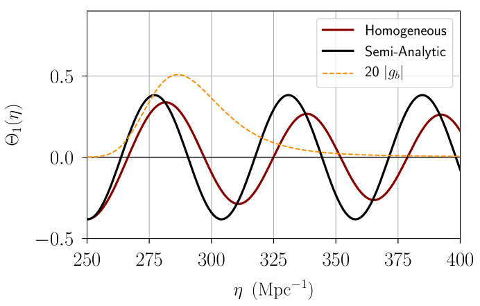
Figure 2: The effects of transient photon-baryon scatterings on $\Theta_{1}$ for $k=0.3h{\rm Mpc}^{-1}$. The red curve includes transients and depicts a numerical evaluation of (4.1). The black curve ignores the effects of transients and depicts the homogeneous part of (4.2). The orange dotted curve plots the (rescaled) baryon visibility function $g_{b}(\eta)$.

Consider the terms in equations (2.10) and (2.14) that describe photon-baryon interactions:

$$\ddot{\Theta}_{0}+\frac{k^{2}}{3}\Theta_{0}=\frac{kR}{3}\dot{v}_{b},\ \quad\ \dot{v}_{b}=\dot{\tau}_{b}(v_{b}-3\Theta_{1}).$$ (4.1)

Since the photons and baryons are not tightly coupled $v_{b}\neq 3\Theta_{1}$. The relative photon-baryon motion induces a drag force on the photon oscillations, which alters their frequency and gives rise to a phase shift.

Ignoring free-streaming effects for the moment, the photon dipole for $\eta>\bar{\eta}$ can be expressed as

$$\Theta_{1}(\eta) =(Ce^{i\omega(\eta-\bar{\eta})}+c.c.)+\Theta^{\rm trans}_{1}(\eta)$$ (4.2)

where $\omega\equiv k/\sqrt{3}$. The first term is the homogeneous solution of (4.1) and $\Theta^{\rm trans}_{1}(\eta)$ parametrizes the correction from transients. The constant $C$ encodes the phase and amplitude of the photons as they transition from the tightly coupled regime to the transient one, and is fixed by matching (4.2) to (3.32) at $\bar{\eta}$:

$$C=-\frac{i}{2\sqrt{3}}(\Theta^{\rm tight}_{0}(\bar{\eta})-\frac{i}{\omega}\dot{\Theta}^{\rm tight}_{0}(\bar{\eta}))\equiv i|\bar{C}|e^{i(kr_{s}(\bar{\eta})+\phi_{\rm tight}(\bar{\eta})+\phi_{\rm match}+\phi_{1}(\bar{\eta}))}e^{-k^{2}/k_{D}^{2}(\bar{\eta})}$$ (4.3)

where $\phi_{\rm match}$ is defined as the phase shift due to the matching and $|\bar{C}|$ is a real number.

The contribution from transients $\Theta^{\rm trans}_{1}(\eta)$ is determined by solving (4.1). While these equations are difficult to solve analytically, the qualitative effects of transients can readily be understood by studying the numerical solution. Figure 2 plots a numerical evaluation of (4.1) against the homogeneous piece of (4.2). We see that the effect of transients is to increase the photon oscillation period. The curve including transients lags behind the homogeneous one, and accumulates a phase shift by the time transients have dissipated. As seen in figure 2, the phase difference is appreciable by the peak of the baryon visibility function. As a result, transients induce a phase shift in the BAO profile.

It turns out that the lifetime of transients $\ddot{\tau}/\dot{\tau}$ is comparable to the oscillation frequencies of modes in the middle of the observable BAO range, $k\sim 0.2\,h\,{\rm Mpc}^{-1}$. Modes whose oscillation periods are longer than the transient lifetime should be less sensitive to the effects of transients. We then expect the size of the BAO phase shift due to transients to be an increasing function of $k$.

4.2 Free-Streaming

As discussed in the previous section, photons are no longer tightly coupled to the baryons after $\bar{\eta}$. Since the photon-baryon scattering rate has decreased, photons begin to free-stream and higher photon multipole moments cannot be neglected. One way to account for free-streaming is by integrating (2.12) to obtain an expression for the full photon temperature fluctuation $\Theta$, and then project out $\Theta_{1}$ as is done in the analysis of the CMB. However, this description hides the fact that free-streaming only induces a perturbative correction to the BAO profile. The BAO is most sensitive to the photon behavior during the era of decoupling, before photons fully enter the free-streaming regime. As a result, contributions from free streaming are better described as a perturbative correction to the (truncated) fluid description where $\Theta_{2}=0$.

The fact that free-streaming effects only provide a small correction to the BAO can be understood by noting that the total comoving distance a free-streaming photon travels during decoupling is of order $\sigma$, the width of the baryon visibility function. This turns out to be less than the comoving wavelengths of observable BAO modes $\lambda\sim 2\pi/k$. Since the photons were originally tightly coupled, individual photons do not travel far during the era of decoupling relative to the BAO length scales. The truncated fluid description is then sufficient for the purposes of determining the BAO, and the effects of free-streaming can be treated as a perturbation.

To derive the corrections from free streaming, we include the term proportional to $\Theta_{2}$ in equation (2.15),

$$\ddot{\Theta}_{0}+\frac{k^{2}}{3}\Theta_{0}=\frac{kR}{3}\dot{v}_{b}+\frac{2k^{2}}{3}\Theta_{2}\ .$$ (4.4)

The solution to (4.4) can be separated into contributions coming from the homogeneous evolution, transients, and free streaming. Using $\Theta_{1}=-\dot{\Theta}_{0}/k$, we find

$$\Theta_{1}(\eta)=(Ce^{i\omega(\eta-\bar{\eta})}+c.c.)+\Theta^{\rm trans}_{1}(\eta)+\Theta^{\rm FS}_{1}(\eta)$$ (4.5)

The behavior of $\Theta^{\rm trans}_{1}(\eta)$ is most sensitive to the dynamics near $\bar{\eta}$, when the transient photon-baryon interactions are largest. Residual photon-baryon scatterings suppress free-streaming around this time. To a good approximation then $\Theta^{\rm trans}_{1}(\eta)$ can be computed using (4.1).

The contribution from free-streaming can be expressed as

$$\Theta^{\rm FS}_{1}(\eta)\equiv-\frac{k}{3}\int_{\bar{\eta}}^{\eta}d\eta^{\prime}e^{i\omega(\eta-\eta^{\prime})}\Theta_{2}(\eta^{\prime})+c.c.$$ (4.6)

We can obtain an expression for $\Theta_{2}$ by first integrating (2.12) for the full photon perturbation and projecting out the quadrupole component. Neglecting contributions from the gravitational potentials, we find

$$\Theta_{2}(\eta) \simeq e^{\tau(\eta)-\tau(\bar{\eta})}(\Theta_{0}(\bar{\eta})j_{2}(k(\eta-\bar{\eta}))+3\Theta_{1}(\bar{\eta})j^{\prime}_{2}(k(\eta-\bar{\eta})))$$ (4.7)

$$\ \ \ \ -\int_{\bar{\eta}}^{\eta}d\eta^{\prime}e^{\tau(\eta)-\tau(\eta^{\prime})}\dot{\tau}(\eta^{\prime})(\Theta_{0}(\eta^{\prime})j_{2}(k(\eta-\eta^{\prime}))+v_{b}(\eta^{\prime})j_{2}^{\prime}(k(\eta-\eta^{\prime}))).$$ (4.8)

Due to the factor of $\dot{\tau}(\eta^{\prime})$, the majority of the integrand’s support comes from the period of time when transient photon-baryon interactions are largest. The integral can then be evaluated using the solutions to (4.1).

To obtain the free-streaming correction to $\Theta_{1}$, we evaluate (4.7) numerically and plug the result into (4.6). Similar to what we found in section 3.3, free-streaming dampens the photon driving force exerted on the baryons and decreases the BAO amplitude. In addition, it induces a scale-dependent phase shift in the BAO profile which becomes larger for modes comparable to the free-streaming length during decoupling $k\sim 2\pi/\sigma$. The correction to the BAO profile due to free-streaming effects should then be largest for modes at the upper end of the observable BAO range.

4.3 Baryon Visibility Function and Baryon Velocity

In section 2.2, the baryon visibility function $g_{b}(\eta)$ was approximated by a Gaussian to obtain $v_{b}(\eta_{g})$. However, this fit does not capture the asymmetric shape of $g_{b}$, which itself induces a phase shift in the BAO. The Gaussian approximation of $g_{b}$ can be improved using a Gaussian Edgeworth expansion. To leading order

$$g_{b}(\eta)\simeq-\frac{1}{\sigma\sqrt{\pi}}e^{-\frac{(\eta-\eta_{*})^{2}}{\sigma^{2}}}(1+k_{3}H_{3}\left(\frac{\eta-\eta_{*}}{\sigma}\right)),\ k_{3}=-\frac{\sigma\sqrt{\pi}\int d\eta g_{b}(\eta)H_{3}(\frac{\eta-\eta_{*}}{\sigma})}{\int d\eta e^{-\frac{(\eta-\eta_{*})^{2}}{\sigma^{2}}}H_{3}(\frac{\eta-\eta_{*}}{\sigma})^{2}}$$ (4.9)

where $H_{3}(x)$ denotes the third Hermite polynomial and $k_{3}$ parametrizes the skewness of $g_{b}$. Figure 3 plots $g_{b}$ obtained numerically against (4.9) and the Gaussian approximation. Clearly (4.9) gives a more accurate fit than the Gaussian approximation. In particular, it does a better job of approximating the peak location and fitting the slowly decaying tail of $g_{b}$.

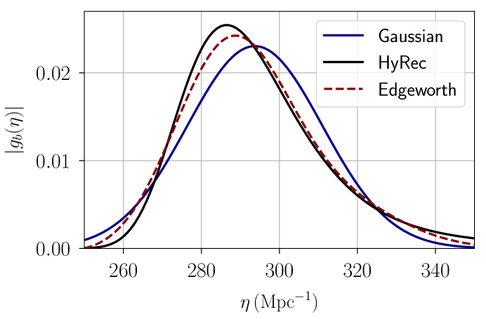
Figure 3: Baryon visibility function $g_{b}(\eta)$. The black curve is obtained numerically from HyRec [50], while the blue and red curves depict (4.9) with and without the skewness parameter $k_{3}$.

We are now in a position to derive an improved formula for $v_{b}(k,\eta_{g})$. By combining the full expression for the photon dipole valid during decoupling (4.5) with (2.22), we find

$$v_{b}(k,\eta_{g})=-3\frac{a(\eta_{*})}{a(\eta_{g})}\int_{-\infty}^{\infty}d\eta g_{b}(\eta)\left[(Ce^{i\omega(\eta-\bar{\eta})}+c.c.)+\Theta^{\rm trans}_{1}(\eta)+\Theta^{\rm FS}_{1}(\eta)\right]+I_{\Phi}(k,\eta_{g})$$ (4.10)

The contributions from $\Theta^{\rm trans}_{1}(\eta)$ and $\Theta^{\rm FS}_{1}(\eta)$ can be evaluated numerically. The piece resulting from the homogeneous evolution of $\Theta_{1}$ can be obtained analytically using (4.9). It is straightforward to evaluate the time integral and find

$$\int_{-\infty}^{\infty}d\eta^{\prime}g_{b}(\eta^{\prime})e^{i\omega(\eta^{\prime}-\bar{\eta})}\simeq-\sqrt{1+k^{2}_{3}(\sigma\omega)^{6}}e^{-\frac{\omega^{2}\sigma^{2}}{4}}e^{i\omega(\eta_{*}-\bar{\eta})+i\phi_{\rm skew}}$$ (4.11)

where $\phi_{\rm skew}\equiv-{\rm tan}^{-1}(k_{3}(\sigma\omega)^{3})$ represents the phase shift due to the skewness of $g_{b}$.

Plugging (4.3) and (4.11) into (4.10) gives the baryon velocity at $\eta_{g}$. We find

$$v_{b}(k,\eta_{g})=-\mathcal{A}_{v_{b}}{\rm sin}(kr_{s}(\eta_{*})+\phi_{v_{b}})+v^{\rm trans}_{b}(k,\eta_{g})+v^{\rm FS}_{b}(k,\eta_{g})+I_{\Phi}(k,\eta_{g})$$ (4.12)

where $v^{\rm trans}_{b}$ and $v^{\rm FS}_{b}$ parametrize the corrections due to transients and free-streaming. The amplitude and phase of the piece due to the homogeneous evolution of $\Theta_{1}$ are

$$\mathcal{A}_{v_{b}} \equiv 6|\bar{C}|\frac{a(\eta_{*})}{a(\eta_{g})}\sqrt{1+k^{2}_{3}(\sigma\omega)^{6}}e^{-k^{2}/k^{2}_{D}(\bar{\eta})}e^{-\frac{\omega^{2}\sigma^{2}}{4}}$$ (4.13)

$$\phi_{v_{b}} \equiv k(r_{s}(\bar{\eta})-r_{s}(\eta_{*})-\frac{\bar{\eta}-\eta_{*}}{\sqrt{3}})+\phi_{\rm tight}(\bar{\eta})+\phi_{\rm match}+\phi_{1}(\bar{\eta})+\phi_{\rm skew}.$$ (4.14)

The first contribution to $\phi_{v_{b}}$ is due to the fact the photons no longer propagate at the speed $c_{s}$ after $\bar{\eta}$. The remaining contributions come from corrections to the tightly coupled photons (LABEL:photon_amplitude_and_phase), matching at $\bar{\eta}$ and the skewness of $g_{b}$. The factors of $v^{\rm trans}_{b}(k,\eta_{g})$ and $v^{\rm FS}_{b}(k,\eta_{g})$ in (4.12) encode phase shifts due to transients and free-streaming. The amplitude of $v_{b}$ is suppressed at large $k$ by diffusion damping. In addition, free streaming during decoupling also decreases the amplitude of $v_{b}(k,\eta_{g})$.

4.4 Baryon Overdensity

As described in section 2.2, the baryon velocity at $\eta_{g}$ gives the leading contribution to the BAO profile. This is due to the velocity overshoot effect, i.e. the fact that the term proportional to $\delta_{b}$ in the expression for $C_{\rm BAO}$ (2.20) is suppressed relative to the term proportional to $v_{b}$ by a factor of $aH/k$. However, in the time between $\bar{\eta}$ and $\eta_{g}$, the baryons have begun to experience gravitational growth and the magnitude of $\delta_{b}$ has increased several times larger than the magnitude of $v_{b}$ by $\eta_{g}$. This partially compensates for the small factor multiplying $\delta_{b}$, which means the contribution from $\delta_{b}$ in (2.20) gives a leading correction to the BAO profile. To derive $\delta_{b}(k,\eta_{g})$, we integrate $\dot{\delta}_{b}=-kv_{b}$ from $\bar{\eta}$ to $\eta_{g}$ and find

$$\delta_{b}(k,\eta_{g}) \simeq 3\Theta_{0}(k,\bar{\eta})+3k\int_{\bar{\eta}}^{\eta_{g}}d\eta\frac{e^{\tau_{b}(\eta)}}{a(\eta)}\int_{-\infty}^{\eta}d\eta^{\prime}a(\eta^{\prime})g_{b}(\eta^{\prime})\Theta_{1}(\eta^{\prime})-k\int_{\bar{\eta}}^{\eta_{g}}d\eta^{\prime}I_{\Phi}(k,\eta^{\prime})$$ (4.15)

where we used $\delta_{b}(\bar{\eta})\simeq 3\Theta_{0}(\bar{\eta})$. It is straightforward to evaluate (4.15) numerically.

5 BAO

Plugging our expressions for the baryon velocity (4.12) and overdensity (4.15) at $\eta_{g}$ into (2.20) yields an improved expression for the BAO

(5.1)

The phase shift $\phi_{v_{b}}$ is due to corrections to the tightly coupled photons (described in section 3) and the skewness of the baryon visibility function (section 4.3). The contributions from transient photon-baryon interactions and free-streaming (sections 4.1 and 4.2) are parametrized by $v^{\rm trans}_{b}$ and $v^{\rm FS}_{b}$. Finally, the contributions from the baryon overdensity $\delta_{b}$ and gravitational potential $I_{\Phi}$ are described in sections 4.4 and 2.2.

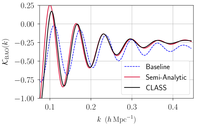
Figure 4: Plot of the baryon growing mode coefficient ${\cal K}_{\rm BAO}=C_{\rm BAO}/(\frac{2k}{5\dot{y}(\eta_{g})}\frac{\Omega_{b}}{\Omega_{m}})$ given by equation (5.1) (red) versus the numerical result (black) obtained with CLASS [47]. The blue curve is the baseline curve describe in equation (2.28), after modifying its amplitude and offset from zero to agree with the amplitude of the third peak and trough obtained with CLASS.

Figure 4 plots $C_{\rm BAO}$ obtained numerically from CLASS [47] against the baseline model (2.28) and our improved semi-analytic model (5.1). The breakdown in the agreement between the semi-analytic model and the output from CLASS at lower $k$ is expected. Our expressions for the contributions from gravitational driving during matter domination and the phase shift due to neutrino anisotropic stress (sections 3.1 and 3.2) rely on $kr_{s}(\eta_{\rm eq})\gg 1$ and $kr_{s}(\eta_{*})\gg 1$, which is more accurate for larger $k$.

Table 1 lists the changes to the first four BAO peak locations in Fourier space due to (from left to right) gravitational driving during matter domination, neutrino anisotropic stresses, higher order corrections to tight coupling, transient photon-baryon interactions, free-streaming of photons, the skewness of the baryon visibility function and the baryon overdensity at $\eta_{g}$. The variations are determined by individually removing each contribution from (5.1) and subtracting the new BAO peak locations from the old ones. For comparison, the last column gives the shifts due to a 1$\%$ shift in the sound horizon at $\eta_{*}$.

As expected, the higher BAO peaks are more sensitive to corrections to tight coupling, transients and free-streaming. The impact of gravitational driving during matter domination is largest in the first peak location. The skewness of $g_{b}$ induces the smallest shifts to the peak locations. The shifts due to the baryon overdensity at $\eta_{g}$ are of similar size as $\delta k_{\nu}$, which is nearly scale-invariant.

The first three entries in Table 1 (left) directly alter the photon distribution around the time of recombination. As a result, these shifts similarly alter the acoustic peaks of the CMB. On average, the neutrino phase is the largest of these effects. At first sight, the weak $k$-dependence of $\delta k_{\nu}$ might appear to contradict the $k$-dependence observed in Figure 3.19. However, because the amplitude of the BAO is also $k$-dependent, the locations of the peaks and the change to the phase are not equivalent. The next four effects in the table (middle) are unique to the BAO and are potentially larger than the neutrino induced phase. These effects are uniquely sensitive to physics during the decoupling of photons and baryons. It would be interesting to explore how these effects might be sensitive to beyond $\Lambda{\rm CDM}$ physics.

The total phase shifts are compared to a one-percent shift in $r_{\rm drift}$ (right columns). Current observations constrain $D_{M}(z)/r_{\rm drift}$ [6] at the percent level and thus are likely already sensitive to these shifts. Next generation surveys such as DESI [8] and Euclid [9] are expected to reach sub-percent level of sensitivity over a larger number of redshift bins, likely translating to a factor of several in improvement in overall sensitivity [51]. These expectations are consistent with forecasts for the measurement of the neutrino phase shift in current and future surveys [30].

peak no.	$\delta k_{\Phi}$	$\delta k_{\nu}$	$\delta k_{\rm tight}$	$\delta k_{\rm trans}$	$\delta k_{\rm free}$	$\delta k_{\rm skew}$	$\delta k_{\delta_{b}}$	$\delta k_{\rm tot}$	$\delta k_{\text{1\%}}$
1st	$3$	$3$	$1$	$-3$	$1$	$-1$	$-4$	$0$	$1$
2nd	$0$	$3$	$1$	$-3$	$0$	$-1$	$-3$	$-3$	$2$
3rd	$0$	$3$	$2$	$-6$	$-4$	$1$	$-3$	$-7$	$3$
4th	$1$	$3$	$4$	$-8$	$-8$	$0$	$-3$	$-11$	$3$

Table 1: BAO peak shifts resulting from corrections to tightly coupled photons and decoupling. Shifts are in units of $10^{-3}h{\rm Mpc}^{-1}$. For comparison, the last column gives the shifts in the peak locations due to a 1$\%$ shift in the sound horizon at $\eta_{*}$.

6 Conclusions and Outlook

In this paper, we presented a detailed analysis of the different physical effects that give rise to the BAO phase in Fourier space, and derived a semi-analytic model for the BAO. This model was used to determine the variations of the BAO peak locations due to seven corrections to the tightly coupled photons and the physics during decoupling. The effects from gravitational driving during matter domination, neutrino anisotropic stresses and higher order corrections to the tight coupling approximation are common to the peak locations of both the CMB and the BAO. The remaining corrections are unique to the physics of baryon decoupling and could, in principle, be altered without impacting the CMB directly. Some of these shifts are comparable in size to the phase shift due to neutrino anisotropic stress or a one-percent shift in the BAO scale, and thus should be large enough to be measured in current and future data.

Our broader motivation for this work is to understand how physics beyond $\Lambda$CDM can alter the BAO non-trivially. This is relevant to the use of the BAO as a standard ruler, since measurements of the BAO phase and peak are degenerate [30, 31]. Our analytic understanding of these phase corrections gives us a window into the types of models that might non-trivially impact the BAO in a way that is not captured by standard BAO analyses. The importance of this is highlighted by the fact that BAO measurements will improve [51] to the point where these phases could be measured with high significance [30]. It would be particularly interesting to investigate whether a direct measurement of the phase of the BAO could be provide new insights into the era of baryon decoupling and any possible new physics that could manisfest itself at that time.

Acknowledgements

We are grateful to Daniel Baumann, Raphael Flauger, Yi Guo, Lloyd Knox, Zhen Pan, Benjamin Wallisch, Matias Zaldarriaga for helpful discussions. We also thank Benjamin Wallisch for providing the numerical template for the neutrino phase shift. D. G. is supported by the US Department of Energy under grant no. DE-SC0019035. A. K. R. is supported by the US Department of Energy under grant no. DE-SC0009919.

Appendix A Matching at Radiation-Matter Equality

In this appendix, we compute the factors of $A_{\rm eq}$ and $B_{\rm eq}$ appearing in (3.32) which represent the contributions to the tightly coupled photons due to the evolution during radiation domination. Ignoring the corrections discussed in section 3, the expression for the tightly coupled photons during matter domination is the homogeneous solution of (2.25) and can be written

$$\Theta_{0}(k,\eta)+\Phi(k,\eta)=-(1-A_{\rm eq}(k)){\rm cos}(kr_{s}(\eta))+B_{\rm eq}(k){\rm sin}(kr_{s}(\eta)).$$ (A.1)

The coefficients $A_{\rm eq}$ and $B_{\rm eq}$ can be fixed by matching (A.1) to the expression for $\Theta_{0}$ valid during radiation domination. Neglecting contributions from matter for the moment, the photon monopole during radiation domination takes the well-known form

$$\Theta^{\rm rad}_{0}(k,\eta)=\frac{2((kr_{s})^{2}-1){\rm sin}(kr_{s})-kr_{s}((kr_{s})^{2}-2){\rm cos}(kr_{s})}{(kr_{s})^{3}}.$$ (A.2)

By matching the functional values and derivatives of (A.1) with (A.2) at $\eta_{\rm eq}$, we find

$$A_{\rm eq}(k)=\frac{kr_{s}(2{\rm sin}(2kr_{s})-kr_{s}({\rm cos}(2kr_{s})-3))-6{\rm sin}^{2}(kr_{s})}{(kr_{s})^{4}}+\Phi{\rm cos}(kr_{s})$$ (A.3)

$$B_{\rm eq}(k)=\frac{(3-(kr_{s})^{2}){\rm sin}(2kr_{s})-2kr_{s}(-(kr_{s})^{2}+{\rm cos}(2kr_{s})+2)}{(kr_{s})^{4}}+\Phi{\rm sin}(kr_{s})$$

where all time dependent functions in (LABEL:matching_coeffs_rad) are evaluated at $\eta_{\rm eq}$ and $\Phi$ is given by (3.4). The phase shift to $\Theta_{0}$ due to the photon evolution during radiation domination is then approximately

$$\phi_{\rm eq}(k)={\rm sin}^{-1}(B_{\rm eq}).$$ (A.4)

Equation (A.2) is only valid if radiation is the only gravitational source during radiation domination. In reality, by $\eta_{\rm eq}$ gravitational collapse has made $\delta$ much larger than $\Theta_{0}$ for the relevant scales. This means that near $\eta_{\rm eq}$, the scale factor and gravitational potentials deviate from their pure radiation domination expressions. While (LABEL:matching_coeffs_rad) gives the leading scale dependence of $A_{\rm eq}$ and $B_{\rm eq}$, the gravitational effects of matter give important corrections. These corrections are difficult to compute analytically, however, it is straightforward to incorporate them by solving (2.5), (2.8) and (2.14) numerically through radiation domination. The results of this are used to evaluate $A_{\rm eq}$ and $B_{\rm eq}$ in (3.32) and (LABEL:photon_amplitude_and_phase).

Appendix B Initial Conditions

In this appendix, we derive the initial conditions for the gravitational potentials including contributions from anisotropic stress using the method described in [44]. Assuming the initial conditions are adiabatic, then at early times the cosmological perturbations can be approximated by the following series solutions,

$$\Phi=\Phi_{0}+\Phi_{2}(k\eta)^{2},\ \Psi=\Psi_{0}+\Psi_{2}(k\eta)^{2},\Theta_{0}=\Theta_{00}+\Theta_{01}(k\eta)+\Theta_{02}(k\eta)^{2},$$ (B.1)

$$N_{0}=N_{00}+N_{01}(k\eta)+N_{02}(k\eta)^{2},\ N_{1}=N_{11}(k\eta)+N_{12}(k\eta)^{2},\ \Theta_{1}=\Theta_{11}(k\eta)+\Theta_{12}(k\eta)^{2},$$ (B.2)

$$N_{2}=N_{22}(k\eta)^{2},\ v_{b}=v_{b1}(k\eta)+v_{b2}(k\eta)^{2}.$$ (B.3)

The series coefficients can be obtained by inserting (B.1) into $\dot{\mathcal{N}}_{2}=\frac{2}{5}k\mathcal{N}_{1}$ and the equations of motion for the metric perturbations and cosmological components given in section 2.1. Matching order by order in $\eta$, we find

$$\Phi_{0}=-(1+\frac{2}{5}\epsilon_{\nu})\Psi_{0},\ \frac{v_{b}}{3}=\Theta_{1}={\mathcal{N}}_{1}=\frac{k\eta}{6}\Psi_{0}.$$ (B.4)

It is useful to write the initial conditions for the gravitational potentials in terms of the conserved scalar curvature perturbation $\zeta$. Using $ik_{i}\delta T^{0}_{i}=4ak(\rho_{\gamma}\Theta_{1}+\rho_{\nu}{\mathcal{N}}_{1})$ and (B.4), we find

$$\zeta\equiv\frac{-ik_{i}\delta T^{0}_{i}H}{k^{2}(\rho+P)}+\Phi=-\frac{3}{2}(1+\frac{4\epsilon_{\nu}}{15})\Psi_{0}.$$ (B.5)

The initial conditions for the gravitational potentials are then

$$\Phi=\frac{2}{3}(1+\frac{2\epsilon_{\nu}}{15})\zeta,\ \Psi=-\frac{2}{3}(1-\frac{4\epsilon_{\nu}}{15})\zeta.$$ (B.6)

References

- [1] D. J. Eisenstein and W. Hu, “Baryonic features in the matter transfer function,” Astrophys. J. 496 (1998) 605, arXiv:astro-ph/9709112.
- [2] SDSS Collaboration, D. J. Eisenstein et al., “Detection of the Baryon Acoustic Peak in the Large-Scale Correlation Function of SDSS Luminous Red Galaxies,” Astrophys. J. 633 (2005) 560–574, arXiv:astro-ph/0501171.
- [3] C. Blake and K. Glazebrook, “Probing dark energy using baryonic oscillations in the galaxy power spectrum as a cosmological ruler,” Astrophys. J. 594 (2003) 665–673, arXiv:astro-ph/0301632.
- [4] BOSS Collaboration, F. Beutler et al., “The clustering of galaxies in the completed SDSS-III Baryon Oscillation Spectroscopic Survey: baryon acoustic oscillations in the Fourier space,” Mon. Not. Roy. Astron. Soc. 464 no. 3, (2017) 3409–3430, arXiv:1607.03149 [astro-ph.CO].
- [5] M. Vargas-Magaña et al., “The clustering of galaxies in the completed SDSS-III Baryon Oscillation Spectroscopic Survey: theoretical systematics and Baryon Acoustic Oscillations in the galaxy correlation function,” Mon. Not. Roy. Astron. Soc. 477 no. 1, (2018) 1153–1188, arXiv:1610.03506 [astro-ph.CO].
- [6] eBOSS Collaboration, S. Alam et al., “The Completed SDSS-IV extended Baryon Oscillation Spectroscopic Survey: Cosmological Implications from two Decades of Spectroscopic Surveys at the Apache Point observatory,” arXiv:2007.08991 [astro-ph.CO].
- [7] Planck Collaboration, N. Aghanim et al., “Planck 2018 results. VI. Cosmological parameters,” arXiv:1807.06209 [astro-ph.CO].
- [8] DESI Collaboration, A. Aghamousa et al., “The DESI Experiment Part I: Science,Targeting, and Survey Design,” arXiv:1611.00036 [astro-ph.IM].
- [9] L. Amendola et al., “Cosmology and fundamental physics with the Euclid satellite,” Living Rev. Rel. 21 no. 1, (2018) 2, arXiv:1606.00180 [astro-ph.CO].
- [10] Z. Pan and L. Knox, “Constraints on neutrino mass from Cosmic Microwave Background and Large Scale Structure,” Mon. Not. Roy. Astron. Soc. 454 no. 3, (2015) 3200–3206, arXiv:1506.07493 [astro-ph.CO].
- [11] R. Allison, P. Caucal, E. Calabrese, J. Dunkley, and T. Louis, “Towards a cosmological neutrino mass detection,” Phys. Rev. D 92 no. 12, (2015) 123535, arXiv:1509.07471 [astro-ph.CO].
- [12] CMB-S4 Collaboration, K. N. Abazajian et al., “CMB-S4 Science Book, First Edition,” arXiv:1610.02743 [astro-ph.CO].
- [13] DES Collaboration, T. Abbott et al., “Dark Energy Survey year 1 results: Cosmological constraints from galaxy clustering and weak lensing,” Phys. Rev. D 98 no. 4, (2018) 043526, arXiv:1708.01530 [astro-ph.CO].
- [14] D. D. Baumann, F. Beutler, R. Flauger, D. R. Green, A. z. Slosar, M. Vargas-Magaña, B. Wallisch, and C. Yèche, “First constraint on the neutrino-induced phase shift in the spectrum of baryon acoustic oscillations,” Nature Phys. 15 (2019) 465–469, arXiv:1803.10741 [astro-ph.CO].
- [15] F. Beutler, M. Biagetti, D. Green, A. z. Slosar, and B. Wallisch, “Primordial Features from Linear to Nonlinear Scales,” Phys. Rev. Res. 1 no. 3, (2019) 033209, arXiv:1906.08758 [astro-ph.CO].
- [16] J. C. Hill, E. McDonough, M. W. Toomey, and S. Alexander, “Early Dark Energy Does Not Restore Cosmological Concordance,” arXiv:2003.07355 [astro-ph.CO].
- [17] O. H. Philcox, M. M. Ivanov, M. Simonović, and M. Zaldarriaga, “Combining Full-Shape and BAO Analyses of Galaxy Power Spectra: A 1.6% CMB-independent constraint on H0,” JCAP 05 (2020) 032, arXiv:2002.04035 [astro-ph.CO].
- [18] Z. Slepian and D. J. Eisenstein, “A Simple Analytic Treatment of Linear Growth of Structure with Baryon Acoustic Oscillations,” Mon. Not. Roy. Astron. Soc. 457 no. 1, (2016) 24–37, arXiv:1509.08199 [astro-ph.CO].
- [19] T. Matsubara, “Resumming Cosmological Perturbations via the Lagrangian Picture: One-loop Results in Real Space and in Redshift Space,” Phys. Rev. D 77 (2008) 063530, arXiv:0711.2521 [astro-ph].
- [20] M. Crocce and R. Scoccimarro, “Nonlinear Evolution of Baryon Acoustic Oscillations,” Phys. Rev. D 77 (2008) 023533, arXiv:0704.2783 [astro-ph].
- [21] N. S. Sugiyama and D. N. Spergel, “How does non-linear dynamics affect the baryon acoustic oscillation?,” JCAP 02 (2014) 042, arXiv:1306.6660 [astro-ph.CO].
- [22] R. A. Porto, L. Senatore, and M. Zaldarriaga, “The Lagrangian-space Effective Field Theory of Large Scale Structures,” JCAP 05 (2014) 022, arXiv:1311.2168 [astro-ph.CO].
- [23] T. Baldauf, M. Mirbabayi, M. Simonović, and M. Zaldarriaga, “Equivalence Principle and the Baryon Acoustic Peak,” Phys. Rev. D 92 no. 4, (2015) 043514, arXiv:1504.04366 [astro-ph.CO].
- [24] D. J. Eisenstein, H.-j. Seo, E. Sirko, and D. Spergel, “Improving Cosmological Distance Measurements by Reconstruction of the Baryon Acoustic Peak,” Astrophys. J. 664 (2007) 675–679, arXiv:astro-ph/0604362.
- [25] N. Padmanabhan, M. White, and J. Cohn, “Reconstructing Baryon Oscillations: A Lagrangian Theory Perspective,” Phys. Rev. D 79 (2009) 063523, arXiv:0812.2905 [astro-ph].
- [26] Y. Noh, M. White, and N. Padmanabhan, “Reconstructing baryon oscillations,” Phys. Rev. D 80 (2009) 123501, arXiv:0909.1802 [astro-ph.CO].
- [27] S. Tassev and M. Zaldarriaga, “Towards an Optimal Reconstruction of Baryon Oscillations,” JCAP 10 (2012) 006, arXiv:1203.6066 [astro-ph.CO].
- [28] H.-M. Zhu, Y. Yu, U.-L. Pen, X. Chen, and H.-R. Yu, “Nonlinear reconstruction,” Phys. Rev. D 96 no. 12, (2017) 123502, arXiv:1611.09638 [astro-ph.CO].
- [29] M. Schmittfull, T. Baldauf, and M. Zaldarriaga, “Iterative initial condition reconstruction,” Phys. Rev. D 96 no. 2, (2017) 023505, arXiv:1704.06634 [astro-ph.CO].
- [30] D. Baumann, D. Green, and B. Wallisch, “Searching for light relics with large-scale structure,” JCAP 08 (2018) 029, arXiv:1712.08067 [astro-ph.CO].
- [31] J. L. Bernal, T. L. Smith, K. K. Boddy, and M. Kamionkowski, “Robustness of baryon acoustic oscillations constraints to beyond-CDM cosmologies,” arXiv:2004.07263 [astro-ph.CO].
- [32] K. Aylor, M. Joy, L. Knox, M. Millea, S. Raghunathan, and W. K. Wu, “Sounds Discordant: Classical Distance Ladder & CDM -based Determinations of the Cosmological Sound Horizon,” Astrophys. J. 874 no. 1, (2019) 4, arXiv:1811.00537 [astro-ph.CO].
- [33] L. Knox and M. Millea, “Hubble constant hunter’s guide,” Phys. Rev. D 101 no. 4, (2020) 043533, arXiv:1908.03663 [astro-ph.CO].
- [34] D. Green et al., “Messengers from the Early Universe: Cosmic Neutrinos and Other Light Relics,” Bull. Am. Astron. Soc. 51 no. 7, (2019) 159, arXiv:1903.04763 [astro-ph.CO].
- [35] S. Bashinsky and U. Seljak, “Neutrino perturbations in CMB anisotropy and matter clustering,” Phys. Rev. D 69 (2004) 083002, arXiv:astro-ph/0310198.
- [36] D. Baumann, D. Green, J. Meyers, and B. Wallisch, “Phases of New Physics in the CMB,” JCAP 01 (2016) 007, arXiv:1508.06342 [astro-ph.CO].
- [37] D. Baumann, D. Green, and M. Zaldarriaga, “Phases of New Physics in the BAO Spectrum,” JCAP 11 (2017) 007, arXiv:1703.00894 [astro-ph.CO].
- [38] D. J. Eisenstein, H.-j. Seo, and M. J. White, “On the Robustness of the Acoustic Scale in the Low-Redshift Clustering of Matter,” Astrophys. J. 664 (2007) 660–674, arXiv:astro-ph/0604361.
- [39] SDSS-III Collaboration, S. Alam et al., “The Eleventh and Twelfth Data Releases of the Sloan Digital Sky Survey: Final Data from SDSS-III,” Astrophys. J. Suppl. 219 no. 1, (2015) 12, arXiv:1501.00963 [astro-ph.IM].
- [40] Z. Pan, L. Knox, B. Mulroe, and A. Narimani, “Cosmic Microwave Background Acoustic Peak Locations,” Mon. Not. Roy. Astron. Soc. 459 no. 3, (2016) 2513–2524, arXiv:1603.03091 [astro-ph.CO].
- [41] R. A. Sunyaev and Y. B. Zeldovich, “Small-Scale Fluctuations of Relic Radiation,” 0Ap&SS 7 no. 1, (Apr., 1970) 3–19.
- [42] W. H. Press and E. T. Vishniac, “Tenacious myths about cosmological perturbations larger than the horizon size,” Astrophys. J. 239 (1980) 1–11.
- [43] W. Hu and N. Sugiyama, “Small scale cosmological perturbations: An Analytic approach,” Astrophys. J. 471 (1996) 542–570, arXiv:astro-ph/9510117.
- [44] C.-P. Ma and E. Bertschinger, “Cosmological perturbation theory in the synchronous and conformal Newtonian gauges,” Astrophys. J. 455 (1995) 7–25, arXiv:astro-ph/9506072.
- [45] S. Dodelson, Modern Cosmology. Academic Press, Amsterdam, 2003.
- [46] P. Meszaros, “The behaviour of point masses in an expanding cosmological substratum,” Astron. Astrophys. 37 (1974) 225–228.
- [47] D. Blas, J. Lesgourgues, and T. Tram, “The Cosmic Linear Anisotropy Solving System (CLASS) II: Approximation schemes,” JCAP 07 (2011) 034, arXiv:1104.2933 [astro-ph.CO].
- [48] J. M. Bardeen, J. Bond, N. Kaiser, and A. Szalay, “The Statistics of Peaks of Gaussian Random Fields,” Astrophys. J. 304 (1986) 15–61.
- [49] M. Zaldarriaga and D. D. Harari, “Analytic approach to the polarization of the cosmic microwave background in flat and open universes,” Phys. Rev. D 52 (1995) 3276–3287, arXiv:astro-ph/9504085.
- [50] Y. Ali-Haimoud and C. M. Hirata, “HyRec: A fast and highly accurate primordial hydrogen and helium recombination code,” Phys. Rev. D 83 (2011) 043513, arXiv:1011.3758 [astro-ph.CO].
- [51] A. Font-Ribera, P. McDonald, N. Mostek, B. A. Reid, H.-J. Seo, and A. Slosar, “DESI and other dark energy experiments in the era of neutrino mass measurements,” JCAP 05 (2014) 023, arXiv:1308.4164 [astro-ph.CO].