A comparison of momentum transport models for numerical relativity

Abstract

The main problems of nonvacuum numerical relativity, compact binary mergers and stellar collapse, involve hydromagnetic instabilities and turbulent flows, so that kinetic energy at small scales lead to mean effects at large scale that drive the secular evolution. Notable among these effects is momentum transport. We investigate two models of this transport effect, a relativistic Navier-Stokes system and a turbulent mean stress model, that are similar to all of the prescriptions that have been attempted to date for treating subgrid effects on binary neutron star mergers and their aftermath. Our investigation involves both stability analysis and numerical experimentation on star and disk systems. We also begin the investigation of the effects of particle and heat transport on post-merger simulations. We find that correct handling of turbulent heating is crucial for avoiding unphysical instabilities. Given such appropriate handling, The evolution of a differentially rotating star and the accretion rate of a disk are reassuringly insensitive to the choice of prescription. However, disk outflows can be sensitive to the choice of method, even for the same effective viscous strength. We also consider the effects of eddy diffusion in the evolution of an accretion disk and show that it can interestingly affect the composition of outflows.

I Introduction

It is progress, of a sort, that the realism of numerical relativity simulations is now limited primarily by the same physical and computational challenges as is that of their Newtonian counterparts. Surely among the greatest of these is the multiscale nature of turbulent fluid flow; kinetic energy at the system size or unstable mode wavelength cascades through an inertial range of smaller scales until finally dissipated into internal energy at scales far below what can be captured numerically. High Reynolds numbers, and hence this turbulent cascade, are expected in all of the main problems in nonvacuum numerical relativity: binary neutron star mergers, black hole-neutron star mergers, core-collapse supernovae, and collapsars.

One solution would be to pursue much higher resolution simulations. The highest resolution binary neutron star mergers have grid spacings of order twenty meters Kiuchi et al. (2015). Meanwhile, several groups are designing computational infrastructure that will allow scaling up to hundreds of thousands of threads (e.g. Kidder et al. (2017)). Another, complementary strategy, is to model subgrid-scale transport effects by adding effective stress, heat and particle conduction, and dynamo terms to the large-scale evolution equations. Several such attempts have been made for relativistic hydrodynamics in the context of binary neutron star post-merger remnants Duez et al. (2004); Giacomazzo et al. (2015); Shibata and Kiuchi (2017); Fujibayashi et al. (2018); Radice (2017) and black hole accretion (also often with post-merger applications) Sadowski et al. (2015); Fujibayashi et al. (2020) and of course in Newtonian hydrodynamics turbulence modeling is a vast endeavor. (For book-length treatments, see Wilcox (2006); Pope (2000). Of particular interest to relativistic astrophysics is the incorporation of turbulence effects on core collapse supernovae that might not be directly captured due to resolution limits or dimensional reduction Murphy and Meakin (2011); Couch and Ott (2015); Radice et al. (2015); Mabanta and Murphy (2018); Couch et al. (2020).) They have the advantage that grids can remain small and simulations cheap, so that parameter explorations can readily be carried out. On the other hand, to be believable, the added terms must be calibrated to and validated by expensive high-resolution simulations. Probably, both strategies will play a role in the successful exploration of turbulent-fluid dynamical-spacetime systems.

An important distinction should be made among subgrid models. (On this distinction, see e.g. Wyngaard (2004)). In what we will call “large-eddy simulations”, it is assumed that a significant portion of the inertial range is resolved, and subgrid stress terms are computed as an extrapolation of the character of resolved turbulence to subgrid scales (e.g. Smagorinsky (1963); Bardina et al. (1980); Grete et al. (2015, 2017)). An example of such methods is the gradient model which has recently been adapted to relativistic magnetohydrodynamics by Carrasco, Viganò, and Palenzuela Carrasco et al. (2020) (see also Viganò et al. (2019)). The subgrid dynamo term of Giacomazzo et al Giacomazzo et al. (2015) might also fit into this category, because the field growth is stopped when the magnetic energy density approaches an estimate of the subgrid turbulent kinetic energy density. Alternatively, one may not resolve the turbulence at all (or fail to model the physics that inputs energy into the turbulent cascade). In this case, subgrid stresses must be assigned as functions of the resolved laminar flow, and one has a mean-field model. (It is common also to introduce new evolution variables in the large-scale evolution representing, for example, the turbulent kinetic energy.) In this paper, we shall mostly be concerned with mean-field models. The most famous is the alpha-viscosity prescription of Shakura and Sunyaev Shakura and Sunyaev (1973), and a number of the above-mentioned numerical relativity studies Duez et al. (2004); Shibata and Kiuchi (2017); Fujibayashi et al. (2018, 2020) follow the alpha-viscosity path of modeling unresolved turbulence as a viscosity via the Navier-Stokes equations. It should be remembered that momentum transport is only one of the large-scale effects of turbulence. By analogy with the kinetic theory of gases, one also expects turbulent heat conduction, turbulent eddy diffusion of scalar quantities like composition variables, and a turbulent effective pressure.

Subgrid transport has recently been introduced into binary neutron star merger simulations by Radice Radice (2017). As described in more detail below, Radice considers his added stress terms to be the results of an averaging procedure with an imposed closure which is similar to but not the same (nor intended to be the same) as the relativistic Navier-Stokes equations. Because his specification of the mixing length does not rely on locally-measured turbulence (most recently, it is calibrated to high-resolution MHD merger simulations Kiuchi et al. (2018)), the resulting model is a mean-field model (a calibrated one) by our definition (although it could be extended into a large eddy model by our definition by using local velocity gradients to estimate the effective viscosity, as done by Smagorinsky and subsequent large-eddy models Smagorinsky (1963)), and so it can be compared to the Navier-Stokes simulations of the Illinois and SACRA groups Duez et al. (2004); Shibata and Kiuchi (2017).

In this paper, we investigate both Navier-Stokes and Radice-style momentum transport models. Our formulations differ from some others in the literature mentioned above in that we retain the same evolution variables as in ideal hydrodynamics, so that the recovery of primitive variables is independent of our various non-ideal transport modifications. We study the proper formulation of both models and analyze their stability. We perform numerical experiments on both of the main configuration types that appear in numerical relativity: a differentially rotating compact star and a neutrino-cooled black hole accretion disk. Finally, we look at the effect of other types of turbulent mixing on a representative accretion disk system. In particular, we consider the effect of turbulent effective heat flows on the mass of the outflow and the effect of eddy diffusion on its composition. The importance of the outflow mass is obvious, but the composition distribution of disk ejecta is also an output of post-merger simulations of great importance for kilonova predictions Metzger (2017), where the relevant composition variable in this case is the electron fraction $Y_{e}$. The lack of turbulent composition mixing in prior studies that model transport by an effective viscosity is potentially one of the major differences between these studies and proper (but expensive) magnetohydrodynamic simulations which incorporate all effects of turbulence. (There are, of course, other major differences, including the effects of a large-scale B field, which no local transport model will be able to capture.)

We find that, in mean-field momentum transport models, it is crucial to properly include turbulent heating to the energy equation. Failure to do so results in unphysical behavior, most notably a nonaxisymmetric instability in rotating stars which often appears only after the star has come close to uniform rotation (so that the effect of the transport is presumed to be nearly done). While simple mean field closure relations are not four-dimensionally covariant, for the types of problems (and coordinate systems) common to numerical relativity, the difference from a Navier-Stokes evolution is quite modest. The only exception, although a very important one, is in the outflow mass, for which the differences can be quite significant. In our test case, heat diffusion significantly increases the mass of ejected matter, while eddy diffusion can affect the peak and width of the $Y_{e}$ distribution.

The paper is organized as follows. In section II, we derive the relativistic Navier-Stokes equations, put them in a convenient form for numerical implementation, and analyze their stability. In section III, we work from a framework of averaging the effects of subgrid stresses, looking particularly at the treatment of the energy equation. In section IV, we test our transport methods on a differentially rotating star problem, first looking at the early-time evolution of the rotation profile and entropy, then at the long-term stability issues. In section V, we present numerical experiments on a black hole accretion system. We summarize our findings in section VI.

II The Relativistic Navier-Stokes Equations

II.1 Metric and Fluid Variables

In the 3+1 formalism, spacetime is foliated into spacelike hypersurfaces $\Sigma(t)$ parametrized by the timelike coordinate $t$. The spacetime metric is $g_{\mu\nu}$, which we decompose as

$$ds^{2}=-\alpha^{2}+\gamma_{ij}(dx^{i}+\beta^{i})(dx^{j}+\beta^{j})$$ (1)

where $\alpha$ is the lapse, $\beta^{i}$ the shift and $\gamma_{ij}$ the 3-metric. The unit normal $n^{\mu}$ to a slice $\Sigma$ is then

$$n^{\mu}=\frac{1}{\alpha}(t^{\mu}-\beta^{\mu})=(1/\alpha,-\beta^{i}/\alpha)\ .$$ (2)

The extrinsic curvature of a slice $\Sigma$ is defined as

$$K_{\mu\nu}=-\nabla_{\nu}n_{\mu}-n_{\nu}\gamma_{\mu}^{\lambda}\nabla_{\lambda}(\ln\alpha)=-\frac{1}{2}\mathcal{L}_{n}\gamma_{\mu\nu}$$ (3)

where $\mathcal{L}_{n}$ is the Lie derivative along the normal $n^{\mu}$.

For a perfect fluid, we define the stress-energy tensor of matter as

$$T^{\mu\nu}=\rho_{0}hu^{\mu}u^{\nu}+Pg^{\mu\nu}$$ (4)

where $\rho_{0}$ is the baryon density, $h=1+P/\rho_{0}+\epsilon$ is the specific enthalpy, $P$ is the pressure and $\epsilon$ the specific internal energy. The 4-velocity $u^{\mu}$ can be decomposed in 3+1 form

$$u^{\mu}=W(n^{\mu}+v^{\mu})$$ (5)

where $W$ is the Lorentz factor, and $v^{\mu}$ the 3-velocity. Note the we require $v^{\mu}n_{\mu}=0$ (i.e. $v^{t}=0$). In components, we have

$$u^{\mu} = (W/\alpha,W[v^{i}-\beta^{i}/\alpha])$$ (6)

$$u_{\mu} = (W[-\alpha+\beta^{i}v_{i}],Wv_{i}).$$ (7)

The conservative variables used for numerical evolutions are

$$\rho_{*} = \rho_{0}W\sqrt{\gamma}$$ (8)

$$\tau = \sqrt{\gamma}n_{\mu}n_{\nu}T^{\mu\nu}-\rho_{*}$$ (9)

$$S_{i} = -\sqrt{\gamma}n_{\mu}\gamma_{i\nu}T^{\mu\nu}.$$ (10)

Although not an evolution variable, the purely spatial projection of the stress tensor appears in source terms.

$$S_{ij}\equiv\alpha\sqrt{\gamma}\gamma^{\alpha}_{i}\gamma^{\beta}_{j}T_{\alpha\beta}$$ (11)

For a perfect fluid, Eq (4), the stress tensor projections are

$$\tau = \rho_{*}(hW-1)-P\sqrt{\gamma}$$ (12)

$$S_{i} = \rho_{*}hu_{i}.$$ (13)

The evolution equations are the conservation of baryon number and the projections of the Bianchi identity $\nabla_{\mu}T^{\mu\nu}=0$:

$$\nabla_{\mu}(\rho_{0}u^{\mu}) = 0$$ (14)

$$\nabla_{\mu}(T^{\mu\nu}n_{\nu}) = T^{\mu\nu}\nabla_{\mu}n_{\nu}$$ (15)

$$\nabla_{\mu}(T^{\mu\nu}g_{\nu i}) = 0\ ,$$ (16)

which can be expanded as

$$\partial_{t}\rho_{*} + \partial_{i}(\rho_{*}v_{T}^{i})=0$$ (17)

$$\partial_{t}\tau + \partial_{i}(\tau v_{T}^{i}+P\sqrt{\gamma}\alpha v^{i})=$$ (18)

$$\alpha PK\sqrt{\gamma}-S^{i}\partial_{i}\alpha+S^{i}S^{j}K_{ij}\frac{\alpha}{\rho_{*}Wh}$$

$$\partial_{t}S_{j} + \partial_{i}(S_{j}v_{T}^{i}+\alpha P\sqrt{\gamma}\delta^{i}_{j})=S_{i}\partial_{j}\beta^{i}$$

$$+\sqrt{\gamma}P(\partial_{j}\alpha+\frac{\alpha\partial_{j}\gamma}{2\gamma})-\rho_{*}Wh\partial_{j}\alpha+\frac{\alpha S^{i}S^{k}\partial_{j}\gamma_{ik}}{2\rho_{*}Wh}$$

where we defined the transport velocity

$$v_{T}^{i}=\frac{u^{i}}{u^{t}}=\alpha v^{i}-\beta^{i}.$$ (20)

For a general stress tensor, the source term for $\tau$ is $-\alpha\sqrt{\gamma}T^{\mu\nu}\nabla_{\nu}n_{\mu}=-S^{i}\partial_{i}\alpha+S_{ij}K^{ij}$, and the source term for $S_{i}$ is $\alpha\sqrt{\gamma}T^{\mu\nu}\partial_{i}g_{\mu\nu}/2$.

II.2 The Shear Tensor

A simple prescription for a viscous fluid is to include a shear viscosity but no bulk viscosity. Then, the stress-energy tensor becomes

$$T^{\mu\nu}=T^{\mu\nu}_{\rm ideal}+\tau^{\mu\nu}=T^{\mu\nu}_{\rm ideal}-2\eta\sigma^{\mu\nu}$$ (21)

where

$$\sigma_{\mu\nu}=\nabla_{(\mu}u_{\nu)}+u^{\alpha}\left(\nabla_{\alpha}u_{(\mu}\right)u_{\nu)}-\frac{1}{3}\nabla_{\alpha}u^{\alpha}h_{\mu\nu}$$ (22)

is the shear tensor and

$$h_{\mu\nu}=g_{\mu\nu}+u_{\mu}u_{\nu}.$$ (23)

The coefficient $\eta$ sets the strength of the viscosity. For a physical viscosity, kinetic theory would lead one to expect $\eta\approx\rho_{0}c_{s}\ell$, where $c_{s}$ is the sound speed and $\ell$ is the mean free path of the constituent particle.

We can take advantage of the identity $\sigma^{\mu\nu}u_{\mu}=0$ to write

$$\sigma_{jt} = -\sigma_{ij}v_{T}^{i}$$ (24)

$$\sigma_{tt} = \sigma_{ij}v_{T}^{i}v_{T}^{j}$$ (25)

$$\sigma^{t}_{i} = \sigma_{ij}\frac{v^{j}}{\alpha}$$ (26)

$$\sigma^{i}_{j} = \sigma_{jk}\left(\gamma^{ik}-\frac{\beta^{i}v^{k}}{\alpha}\right)$$ (27)

$$\sigma^{t}_{t} = -\sigma_{ij}\frac{v^{i}_{T}v^{j}}{\alpha}$$ (28)

$$\sigma^{tt} = \frac{\sigma_{ij}}{\alpha^{2}}v^{i}v^{j}$$ (29)

$$\sigma^{ti} = \left(\frac{\gamma^{ik}}{\alpha}-\frac{\beta^{i}v^{k}}{\alpha^{2}}\right)\sigma_{kj}v^{j}$$ (30)

$$\sigma^{ij} = \sigma_{lm}\left(\gamma^{il}\gamma^{jm}+\frac{\beta^{i}\beta^{j}}{\alpha^{2}}v^{l}v^{m}\right)$$ (31)

$$-\sigma_{lm}\left(\frac{\beta^{i}}{\alpha}\gamma^{jl}v^{m}+\frac{\beta^{j}}{\alpha}\gamma^{il}v^{m}\right),$$

and we only need to compute $\sigma_{ij}$ to recover the full 4-dimensional tensor. This 3D tensor can be simplified as

$$\sigma_{ij} = \frac{W}{2\alpha}\left(u_{j}\partial_{t}u_{i}+u_{i}\partial_{t}u_{j}\right)-\frac{h_{ij}}{3\alpha\sqrt{\gamma}}\partial_{t}(\sqrt{\gamma}W)$$

$$+ \frac{1}{2}\left(\partial_{i}u_{j}+\partial_{j}u_{i}\right)-\frac{h_{ij}}{3\alpha\sqrt{\gamma}}\partial_{k}(W\sqrt{\gamma}v^{k}_{T})$$

$$- W(K_{ij}+v_{k}\Gamma^{(3)k}_{ij})-\frac{W}{2\alpha}(u_{i}\partial_{j}u_{t}+u_{j}\partial_{i}u_{t})$$

$$+ \frac{Wv^{k}_{T}u_{i}}{2\alpha}(\partial_{k}u_{j}-\partial_{j}u_{k})+\frac{Wv^{k}_{T}u_{j}}{2\alpha}(\partial_{k}u_{i}-\partial_{i}u_{k})$$

where $\Gamma^{(3)k}_{ij}$ are the 3-dimension Christoffel symbols associated with $\gamma_{ij}$. The above expression only requires time derivatives of $u_{i}$ and $(\sqrt{\gamma}W)$.

II.3 Evolution Equations

The inclusion of the viscous shear tensor induces modification to the evolution equation for $\tau$ and $S_{i}$. The fluxes are now

$$F^{i}_{\tau} = \tau v^{i}_{T}+P\alpha\sqrt{\gamma}v^{i}-2\eta\alpha^{2}\sqrt{\gamma}\sigma^{ti}$$ (33)

$$F^{i}_{S_{j}} = S_{j}v_{T}^{i}+\alpha P\sqrt{\gamma}\delta^{i}_{j}-2\eta\alpha\sqrt{\gamma}\sigma_{j}^{i}$$ (34)

and the source terms

$$S_{\tau} = S_{\tau}^{\rm ideal}-2\eta\alpha\sqrt{\gamma}(\sigma_{ij}K^{ij}-\sigma^{ti}\partial_{i}\alpha)$$ (35)

$$+ \partial_{t}(2\eta\alpha^{2}\sqrt{\gamma}\sigma^{tt})$$

$$S_{S_{j}} = S_{S_{j}}^{\rm ideal}-\eta\alpha\sqrt{\gamma}\sigma^{\mu\nu}\partial_{j}g_{\mu\nu}$$ (36)

$$+ \partial_{t}(2\eta\alpha\sqrt{\gamma}\sigma_{j}^{t})\ ,$$

where $S_{\tau}^{\rm ideal}$ and $S_{S_{j}}^{\rm ideal}$ are the source terms for ideal hydrodynamcs, given as the right-hand sides of equations (18) and (II.1), respectively.

II.4 Stability

We will consider stability on a flat background, for perturbation around a homogeneous fluid configuration. The perturbations will be planar waves proportional to $\exp{(\Gamma t+ikx)}$. First order theories of the Navier-Stokes equation, including the equations derived in the previous section, are acausal and have unstable modes with extremely rapid growth rate Hiscock and Lindblom (1983). One can however recover a stable and covariant viscous formalism by going to second-order methods (Israel-Stewart viscosity Israel (1976); Israel and Stewart (1979); Hiscock and Lindblom (1983)), which treat the viscous stress-tensor as an evolved variable.

Suppose that at a particular instant in time, the viscous coefficient $\eta$ is a function of the local density $\rho_{0}$ and temperature $T$, while the shear tensor is a function of $u^{\mu}$ and its derivatives. Then the instantaneous values of $-2\eta\sigma_{ij}$ at event $x^{\mu}$ are

$$\tau_{ij}^{\rm inst}(x^{\mu})=-2\eta(\rho_{0}(x^{\mu}),T(x^{\mu}))\sigma_{ij}(u^{\alpha}(x^{\mu}),\partial_{\beta}u^{\alpha}(x^{\mu}))\ ,$$

Instead of setting the viscous stress tensor $\tau_{ij}$ at each event $x^{\mu}$ equal to $\tau_{ij}^{\rm inst}(x^{\mu})$, we evolve $\tau_{ij}$ according to

$$\partial_{t}\tau_{ij}=-\frac{1}{t_{d}}\left(\tau_{ij}-\tau_{ij}^{\rm inst}\right)$$ (37)

or

$$\mathcal{L}_{\vec{t}+\vec{v_{T}}}\tau_{ij}=-\frac{1}{t_{d}}\left(\tau_{ij}-\tau_{ij}^{\rm inst}\right)$$ (38)

The advection term in the second version is probably preferable for systems with high velocities (at least, high velocities not along a symmetry of the fluid configuration). Alternatively, if $t_{d}$ is small compared to physical timescales, the driver can handle the advection itself. In the applications in this paper, systems are mostly axisymmetric and velocities mostly azimuthal, so we find better performance with Eq. (37).

Consider the case of a perturbation propagating along the direction of the fluid motion ($u_{y}=u_{z}=0$, $u_{x}\neq 0$). We perturb the energy and momentum equations and close the system by specifying an equation of state $\epsilon(\rho_{0},T)$, $P(\rho_{0},T)$. Consider transverse modes (involving $\delta u_{A}$, $\delta\tau_{xA}$), where capital roman letters will stand for indices $y,z$. We have the constraint

$$\delta\tau^{t\mu}=\frac{u_{x}}{W}\delta\tau^{x\mu}.$$ (39)

The perturbed momentum equation along $y,z$ becomes

$$\rho_{0}h(\Gamma W+iku_{x})\delta u_{A}+(\Gamma\frac{u_{x}}{W}+ik)\delta\tau_{xA}=0$$

and the evolution equations for $\delta\tau_{xA}$ without advection term is

$$(\Gamma t_{d}+1)\delta\tau_{xA}=-\eta W(ikW+u_{x}\Gamma)\delta u_{A}.$$ (40)

With the advection term, it would be

$$(\Gamma t_{d}+1)\delta\tau_{xA}=-\eta W(ikW+u_{x}\Gamma)\delta u_{A}-\frac{u_{x}}{W}t_{d}ik\delta\tau_{xA}.$$ (41)

Concentrating for the moment on the system without advection of $\tau_{xA}$ (Eq. (40)), we thus have the system

$$\begin{pmatrix}\rho_{0}h(\Gamma W+iku_{x})&\frac{1}{W}(\Gamma u_{x}+ikW)\\ \eta W(ikW+u_{x}\Gamma)&1+\Gamma t_{d}\end{pmatrix}\begin{pmatrix}\delta u_{A}\\ \delta\tau_{xA}\end{pmatrix}=\begin{pmatrix}0\\ 0\end{pmatrix}$$ (42)

Taking the determinant of the matrix and setting it equal to zero, we solve for $\Gamma$ and find

$$\Gamma=\frac{-\rho_{0}hW+i(\cdots)\pm\Delta^{1/2}}{\cdots}\ ,$$ (43)

where we have neglected to expand factors not relevant to the question of stability, which requires only $\Re{(\Gamma)}<0$. In the above,

$$\Delta = (\rho_{0}hW)^{2}$$ (44)

$$- 2iku_{x}\rho_{0}h\left(\rho_{0}hWt_{d}+2\eta\right)$$

$$- k^{2}\left((\rho_{0}hu_{x}t_{d})^{2}+4\eta W\rho_{0}ht_{d}\right).$$

For stability, we need $\Re{\left(\Delta^{1/2}\right)}\leq\rho_{0}hW$. Note that the marginal stability case $\Re{\Delta^{1/2}}=\Re{\Delta_{\rm ms}^{1/2}}=\rho_{0}hW$ is of the form $\Delta_{\rm ms}=(\rho_{0}hW\pm ikB)^{2}=(\rho_{0}hW)^{2}\pm 2ik\rho_{0}hWB-k^{2}B^{2}$ for some $B\in\mathbb{R}$. On the other hand, Eq. (44) has the form $\Delta=(\rho_{0}hW)^{2}-2ik\rho_{0}hWC-k^{2}D$ for $C$,$D\in\mathbb{R}$. Thus, $D=C^{2}$ is the condition for marginal stability, while $D>C^{2}$ is the condition for stability, which can be written

$$(\rho_{0}hu_{x}t_{d})^{2}+4\eta W\rho_{0}ht_{d}>\frac{u_{x}^{2}}{W^{2}}(\rho_{0}hWt_{d}+2\eta)^{2}$$ (45)

or

$$t_{d}>\frac{W}{\rho_{0}h}\left(\eta\frac{W^{2}-1}{W^{2}}\right)\ ,$$ (46)

which shows that $t_{d}>0$ is required whenever $\eta\neq 0$.

One can repeat the above analysis with the advection term and arrive at exactly the same condition.

II.5 Implementation

The Israel-Stewart formulation of the Navier-Stokes equations can be implemented in a numerical relativity code in either of two ways. First, one can retain the general definition of $\tau$ and $S_{i}$ in terms of the total stress tensor, Eq. (9) and (10), which would then include viscous terms. In this case, the algorithm for recovering primitive variables must be altered. This is the method chosen by Fujibayashi et al Fujibayashi et al. (2018). Second, one could retain the definition of $\tau$ and $S_{i}$ in terms of fluid variables, Eq. (12) and (13) in which case all terms from the divergence of the viscous stress tensor are regarded as source or flux terms. In this case, primitive variable recovery is not affected by viscosity, but the viscous source terms require knowing the time derivatives $\partial_{t}(\sqrt{\gamma}W)$ and $\partial_{t}u_{i}$. We choose this second method. The needed time derivatives are estimated by storing $\sqrt{\gamma}W$ and $u_{i}$ at the previous timestep and then computing at each step $k$ the backward-centered time derivative $\partial_{t}X(t_{k})=[X(t_{k})-X(t_{k-1})]/(t_{k}-t_{k-1})$.

Second-order theories of viscosity also require the evolution of the stress tensor. We promote $A_{ij}\equiv-2\eta\sigma_{ij}W\sqrt{\gamma}$ to be a new evolved variable with evolution equation

$$\partial_{t}A_{ij}+\mathcal{A}_{ij}=-\frac{A_{ij}-A_{ij}^{\rm inst}}{t_{d}u^{0}}$$ (47)

where $\mathcal{A}_{ij}$ is an optional advective term $\mathcal{L}_{v_{T}}A_{ij}$.

We evolve Eq. (37) using implicit time steps. This can be written clearly if we momentarily suppress indices and use subscripts for timesteps, so that $A_{k}$ is a component of $A_{ij}$ at step $k$. Given $A_{k-1}$ and $A^{\rm inst}_{k}$, we take a step of size $\Delta t=t_{k}-t_{k-1}$ by

$$A_{k}=\frac{A_{k-1}+A^{\rm inst}_{k}\Delta t/(u^{0}t_{d})-\mathcal{A}(A_{k-1})\Delta t}{1+\Delta t/(u^{0}t_{d})}$$ (48)

We have experimented with the choice of $t_{d}$, setting it to some fraction of the dynamical timescale–a constant for star runs, a fraction of the local Keplerian period for disk runs. We find our results to be insensitive to its value so long as $t_{d}$ is small compared to the dynamical timescale and the instability is not triggered (cf. Eq. (46)).

We add an option to suppress viscosity at low densities or very close to the black hole, anticipating the possibility of excess artificial viscous heating in these regions. From Eq. (46), the minimum $t_{d}$ scales with $\eta$, so if we suppress $\eta$ by some function of density or distance from the black hole, we reduce $t_{d}$ by the same factor.

II.6 Other Covariant Implementations

The procedure of promoting viscous stress to an independent evolved variable can be extended to other dissipative fluxes (heat flux, etc), a process done systematically in the field of extended irreversible thermodynamics Jou et al. (1988). However, even the Israel-Stewart theory is known to incorrectly handle strong shocks Olson and Hiscock (1990); Geroch and Lindblom (1991), which could be a serious problem in some numerical relativity applications. A different way of improving the behavior of the relativistic Navier-Stokes equations, explored by Lichnerowicz Lichnerowicz (1955) and Disconzi Disconzi (2014), is to replace $u_{i}$ by $hu_{i}$ in the formula for the shear tensor.

Recently, a new formulation of relativistic viscous hydrodynamics has been introduced by Bemfica, Disconzi, Noronha, and Kovtun (BDNK) Bemfica et al. (2018, 2019, 2020). They begin from a general expansion of the stress tensor in covariant terms with first derivatives of fluid variables. Each term will be multiplied by a coefficient, and BDNK find conditions on the coefficients that guarantee stability and causality. Kinetic theory determines some coefficients, but freedom remains in the choice of others, different values representing different choices in the definition of fluid variables out of equilibrium. Presumably, a similar procedure could be followed to model turbulent effective stresses, with similar freedoms reflecting different ways to average over small-scale eddies. However, the BDNK formulation has not yet been used in numerical relativity.

In this paper, we restrict attention to momentum transport methods already in use in numerical relativity, which is already enough to get some indication of how sensitive simulations are likely to be to the choice of method.

III Effective Reynolds Stress from Subgrid-Scale Turbulence

III.1 Filtered Variables and Evolution Equations

As was pointed out by Boussinesq and Prandtl over a century ago, the mixing of momentum by turbulent eddies is analogous to molecular transport in a gas, suggesting that on scales much larger than the eddies, the mean stress from turbulence might be like a viscosity. Once again, we would expect $\eta_{T}\approx\rho_{0}c_{s}\ell$, but now $\ell$ is the mixing length associated with the turbulence.

To pursue the kinetic theory analogy, divide the velocity flow into large and small scales: $v^{i}=\overline{v}^{i}+\delta v^{i}$. The two components are defined by an averaging / low-pass filtering operator $\langle\cdots\rangle$, such that $\langle v^{i}\rangle=\overline{v}^{i}$, $\langle\delta v^{i}\rangle=0$. Then one applies the filter to the ideal energy and momentum equations to obtain evolution equations for $\overline{\tau}$ and $\overline{S}_{i}$.

The subleties that arise can be illustrated in the case of Minkowski spacetime and incompressible small-scale turbulence. Then the filtered equations can be written

$$\partial_{t}\overline{S}_{i}+\partial_{j}(\overline{S_{i}v^{j}}+\delta_{i}^{j}P) = 0$$

$$\partial_{t}\overline{\tau}+\partial_{j}[\rho_{0}h\overline{Wv^{j}}-\rho\overline{v}^{j}] = 0$$

where $\overline{S}_{i}=\rho h\overline{Wv_{i}}$. Note that $\overline{S_{i}v^{j}}\neq\overline{S}_{i}\overline{v}^{j}$ and $\overline{Wv_{i}}\neq\overline{W}\overline{v}_{i}$. Assuming $\delta v^{i}$ is not highly relativistic, we can Taylor expand the Lorentz factor in $\delta v^{i}$ and get $\overline{W}=W(\overline{v}^{i})$, $\delta W=\overline{W}^{3}\overline{v}^{j}\delta v_{j}$. Then

$$\langle v^{i}W\rangle=\overline{W}\overline{v}^{i}+\overline{W}^{3}\overline{v}^{j}\left\langle\delta v_{j}\delta v^{i}\right\rangle\ ,$$

Similarly, we define

$$\langle S_{i}v^{j}\rangle\equiv\overline{S}_{i}\overline{v}^{j}+\tau_{i}{}^{j}\ ,$$ (49)

where we now redefine $\overline{S}_{i}$ to be $S_{i}(\overline{v}_{i})\neq\langle S_{i}\rangle$. This redefinition is desirable because it preserves the relationship between primitive and conservative variables at the filtered level. One finds $\tau_{i}{}^{j}$ to be

$$\tau_{i}{}^{j}=\rho_{0}h\overline{W}\langle\delta v_{i}\delta v^{j}\rangle+O(|\overline{v}|^{2}\times\langle\delta v\delta v\rangle)$$

with the omitted terms coming from correlation between $\delta W$ and $\delta v$. To second order in $\overline{v}^{i}$, $\tau_{ij}$, we have

$$\partial_{t}\overline{S}_{i}+\partial_{j}(\overline{S}_{i}\overline{v}^{j}+\tau_{i}{}^{j}) = 0$$ (50)

$$\partial_{t}\overline{\tau}+\partial_{j}(\overline{S}^{j}+\overline{v}^{k}\tau_{k}{}^{j}) = 0$$ (51)

Note that the extra term in the energy equation, from the difference between the redefined $\overline{S}_{i}$ and $\langle S_{i}\rangle$, is necessary to correctly recover the Newtonian limit, and in particular to secure energy conservation in this limit. One could handle this instead by adding the $\tau\cdot v$ term to the definition of the conservative variable $\overline{S}_{i}$, i.e. by keeping the definition $\overline{S}_{i}=\langle S_{i}\rangle$, but we find it more straightforward to retain the standard relations between primitive and conservative variables.

Returning to the case of general metric and relativistic mean velocities, the cleanest way to obtain the transport terms proportional to the mean velocity is to impose that $\tau_{ij}$ be the spatial components of a 4D tensor that obey the usual orthogonality conditions for a shear tensor: $\tau_{\mu\nu}u^{\nu}=0$. Then the added terms to the energy and momentum flux are the same as in equations (34) and (33), with $\tau^{\alpha\beta}=-2\eta\sigma^{\alpha\beta}$ and with $\sigma^{i}_{j}$ and $\sigma^{ti}$ related to $\sigma_{ij}$ as in Eq. (27) and (30).

To test the effect of the velocity-dependent terms, we write these terms as

$$\partial_{t}\tau = \cdots-\partial_{j}[(k_{1}\alpha\gamma^{jk}-k_{2}\beta^{j}v^{k})v^{l}\tau_{kl}]$$

$$+\alpha\sqrt{\gamma}\gamma^{ki}\gamma^{lj}K_{kl}\tau_{ij}$$

$$\partial_{t}S_{i} = \cdots-\partial_{j}[\sqrt{\gamma}\tau_{im}(\alpha\gamma^{mj}-k_{2}\beta^{j}v^{m})]$$

$$+\frac{1}{2}\sqrt{\gamma}\tau_{jk}(-2k_{2}v^{j}v^{k}\partial_{i}\alpha+2k_{2}v^{k}\partial_{i}\beta^{j}-\alpha\partial_{i}\gamma^{jk})\ ,$$

where “$\cdots$” indicates the perfect fluid terms, and $k_{1}$, $k_{2}$ are constants. To enforce $\tau_{\mu\nu}u^{\nu}=0$, these constants should be $k_{1}=k_{2}=1$. $k_{1}=1$, $k_{2}=0$ has only the term needed to recover the Newtonian limit. $k_{1}=k_{2}=0$ would be to take equations (8) and (9) from Radice (2017) while not accounting for the difference between $S_{i}(\langle v_{i}\rangle)$ and $\langle S_{i}\rangle$ (which is the formalism used in Radice (2017, 2020)).

One can carry out a stability analysis as in Section II.4 for the above mean-field turbulence theory. Because $\tau$ no longer appears under the time derivative in the left-hand side of the momentum equation, the $\Gamma u_{x}/W$ term in the upper right hand entry of the matrix in Eq. (42) is no longer present. Anticipating that $t_{d}>0$ will no longer be required, we can set $t_{d}=0$ and solve a linear equation for $\Gamma$, finding the real part to be unconditionally negative.

III.2 The Closure Condition

Guided by the Smagorinsky closure Smagorinsky (1963) of Newtonian turbulence modeling, Radice Radice (2017) proposes the following relativistic closure

$$\tau_{ij}=-2\nu\rho_{0}hW^{2}\left[\frac{1}{2}(\nabla_{i}\overline{v}_{j}+\nabla_{j}\overline{v}_{i})-\frac{1}{3}\nabla_{k}\overline{v}^{k}\gamma_{ij}\right]\ ,$$ (54)

where $\nabla_{i}$ is the 3D covariant derivative compatible with $\gamma_{ij}$.

In a large-eddy simulation (as defined above), $\nu$ would be set by the local state of the turbulence as determined by difference operators on the smallest resolved scales. This requires the simulation to resolve some of the inertial range of the turbulence. A mean field model is needed if the turbulence is totally unresolved or if the physics driving the turbulence is missing in the simulation. For example, if turbulence is driven by the magnetorotational instability and one’s simulation does not include magnetic fields, one would need a mean field closure condition even if the hypothetical MRI wavelength is resolved. The natural choice is

$$\nu=\ell c_{s}$$ (55)

with $\ell$ the mixing length.

The evolution equations with the above closure are not–and are not meant to be–exactly equivalent to the Navier-Stokes equations. Nevertheless, Eq. (54) clearly does closely resemble a viscous stress and behaves in a similar way.

The model is completed by choosing the mixing length $\ell$. This will depend on the system; the focus of Radice’s work was binary neutron stars. In his original paper, he used constant values of $\ell$ set to be similar to the wavelength of the fastest growing MRI mode for $B\sim 10^{14}$–$10^{15}$G. More recently Radice (2020), he has used a density-dependent $\ell(\rho_{0})$, where the function $\ell(\rho_{0})$ was fit to the results of high-resolution MHD simulations of binary neutron star mergers by Kiuchi et al Kiuchi et al. (2018).

III.3 The Issue of Covariance

Equation (54) is covariant with respect to spatial coordinate transformations, but not with regard to general spacetime coordinate transformations, a point made by Radice himself. The filtering operator is itself frame/slicing dependent, so we should not expect general covariance in the final equations . However, “not covariant” does not necessarily mean “not valid”. Similar points are made by Carrasco et al Carrasco et al. (2020) with regard to their relativistic subgrid code. Since theirs is a large-eddy code, they also point out that discretization for finite differencing itself violates covariance in the same way and to a similar degree. Also, covariance is regained in their case, but not in the mean field case, in the limit of infinite resolution, albeit trivially so because the subgrid terms then disappear.

However, a non-covariant choice of closure may leave coordinate-independent artifacts. For example, one physically expects that, when the radius of curvature is larger than the mixing length, momentum transport should operate only when there is a nonzero shear as measured in a local Lorentz frame, and heating should occur if and only if $\sigma^{\alpha\beta}\sigma_{\alpha\beta}\neq 0$. This is guaranteed for the relativistic Navier-Stokes equations but not for Eq. (54).

Hereafter, we will refer to evolutions with the full Navier-Stokes equations, stabilized by evolving the spatial stress tensor with the driver equation (47), as “Navier-Stokes” or “NS” evolutions. Mean-field turbulence evolutions using the closure equation (54) will be called “turbulent mean stress” or “TMS” evolutions.

III.4 Diffusion of scalar quantities

In addition to transporting momentum, turbulence leads to other effects that can be understood qualitatively as transport by “mixing”. These include eddy diffusion of particle species and turbulent heat transport. 

We consider only the first of these effects. We consider a scalar quantity $Y$, say a species fraction that (up to reaction source terms) advects with the fluid, so that $\rho_{*}Y$ obeys a continuity equation (possibly with reaction source terms). Turbulent mixing will produce a flux of $\rho_{*}Y$ which we take to be $F_{\rho Y}\approx\rho_{0}c_{s}\ell_{D}\nabla Y$, where we have given ourselves the freedom of using a different mean free path for momentum transport and diffusion: $\ell_{D}\equiv\lambda_{D}\ell$ for some constant $\lambda_{D}$. Taking the divergence of this flux (and ignoring the time derivative term), we get

$$\partial_{t}(\rho_{*}Y)+\partial_{i}(\rho_{*}Yv_{T}^{i})=\partial_{j}(\rho_{*}c_{s}\ell_{D}\partial^{j}Y)+\cdots,$$ (56)

where the ellipsis $\cdots$ indicates the other source terms.

As with the TMS stress, this flux is not 4-dimensionally covariant. A covariant treatment would be, for example,

$$\nabla_{\mu}\mathcal{Y}^{\mu} = 0$$ (57)

$$\mathcal{Y}^{\mu} = \rho_{0}Yu^{\mu}-\rho_{0}c_{s}\ell_{D}(g^{\mu\nu}+u^{\mu}u^{\nu})\nabla_{\nu}Y$$ (58)

as can easily be seen by going into a comoving local Lorentz frame.

Heat transport might be modeled in a similar way. Since eddies (except near the dissipation scale) evolve adiabatically, specific entropy $s$ rather than temperature would seem to be the more appropriate scalar quantity to diffuse. This would be in keeping with the normal practice in mixing length theory treatments of convective stars (e.g. Ruediger (1989)), although here there is no presumption that eddies are buoyancy driven. This could be captured by a turbulent mean heat flux $q_{i}=\rho_{0}Tc_{s}\ell_{S}\nabla_{i}s$ for some $\ell_{S}\equiv\lambda_{S}\ell$. The corresponding covariant 4-vector obeying $q\cdot u=0$ is $q_{\mu}=\rho_{0}Tc_{s}\ell_{S}(\nabla_{\mu}s+u^{\nu}u_{\mu}\nabla_{\nu}s)$. In the spirit of TMS, we eliminate time derivatives by assuming entropy roughly advects $u^{\nu}\nabla_{\nu}s\approx 0$ (as would be exactly true if it were a perfect fluid in the absence of shocks and radiation). Then

$$q_{\alpha} = \rho_{0}Tc_{s}\ell_{S}(-v_{T}^{i}\nabla_{i}s,\nabla_{i}s)$$ (59)

$$T^{\mu\nu}_{\rm heat} = q^{\mu}u^{\nu}+q^{\nu}u^{\mu}$$ (60)

$$F_{\tau}^{i} = \cdots+\alpha W\sqrt{\gamma}(q^{i}+v_{T}^{i}q^{t})$$ (61)

$$F_{S_{j}}^{i} = \cdots+\alpha\sqrt{\gamma}(q^{i}u_{j}+q_{j}u^{i})$$ (62)

$$S_{\tau} = \cdots-S^{i}_{\rm heat}\partial_{i}\alpha+S^{ij}_{\rm heat}K_{ij}$$ (63)

$$S_{S_{j}} = \cdots+\frac{1}{2}\alpha\sqrt{\gamma}T^{\mu\nu}_{\rm heat}\partial_{i}g_{\mu\nu}\ ,$$ (64)

where $S^{i}_{\rm heat}$ and $S^{ij}_{\rm heat}$ are projections of $T^{\mu\nu}_{\rm heat}$ as in Eq. (10) and (11), and indices of the heat flux and 4-velocity are raised and lowered using the 4-metric.

Simulations of magnetorotational turbulence find that the momentum transport is dominated by average Maxwell rather than average Reynolds stress, with the former around a few times larger than the latter (e.g. Hawley et al. (1995); Brandenburg et al. (1995); Stone et al. (1996)). This suggests that $\lambda_{D}=\lambda_{S}=1$ probaby overestimates mixing effects. The choice of setting all mixing lengths equal, used at times below, is a useful way of checking what sort of influence turbulent particle diffusion and heat flux might have.

IV Test on a differentially rotating star

IV.1 Axisymmetric heating

From an astrophysicists’s point of view, turbulence is important primarily for two reasons. First, it transports angular momentum. Second, it transfers kinetic energy to small enough scales for it to be dissipated away as heat. Under the influence of a shear viscosity, a differentially rotating star will approach uniform rotation on the viscous timescale $\sim R^{2}/\nu$, where $R$ is the characteristic length of the shear flow, in this case the radius of the star. The fluid will acquire entropy at a rate

$$nT\frac{ds}{dt_{\rm prop}}=2\eta\sigma_{\alpha\beta}\sigma^{\alpha\beta}\ ,$$ (65)

where $n$, $T$, $s$, and $t_{\rm prop}$ are the number density, temperature, specific entropy, and proper time along the fluid element, respectively. For a Gamma-law equation of state $P=(\Gamma-1)\rho_{0}\epsilon$, $P(T=0)=\kappa\rho_{0}^{\Gamma}\equiv P_{\rm cold}$ this can be written

$$nT\frac{ds}{dt_{\rm prop}} = \frac{P_{\rm cold}}{\Gamma-1}\frac{d}{d\tau}\left(\frac{P}{P_{\rm cold}}\right)$$ (66)

$${\partial_{t}}({E}_{\ast}) = -{\partial_{j}}({E}_{\ast}{v}_{T}^{j})$$

$$+ {\frac{\alpha\sqrt{\gamma}}{\Gamma}}(\frac{E_{\ast}}{W\sqrt{\gamma}})^{(1-\Gamma)}({2\eta}{\sigma_{\alpha\beta}}{\sigma^{\alpha\beta}})$$

Where $E_{\ast}{\equiv}W\sqrt{\gamma}(\rho_{0}\epsilon)^{1/\Gamma}=W\sqrt{\gamma}(\frac{P}{\Gamma-1})^{1/\Gamma}$ Baumgarte and Shapiro (2010).

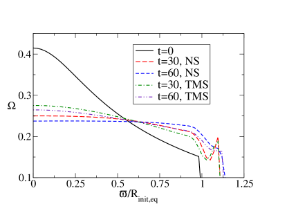
Figure 1: Equatorial angular velocity $\Omega$ at three times for NS and TMS evolution. Angular velocity is shown as a function of coordinate cylindrical radius $\varpi$, normalized to the initial equatorial radius $R_{\rm init,eq}$.

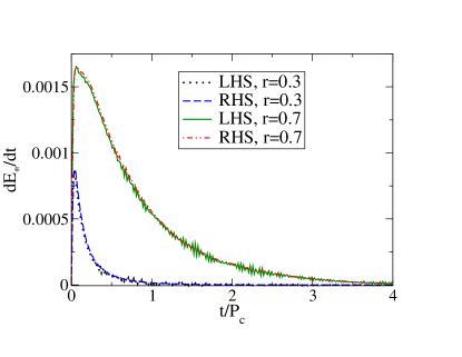
Figure 2: Time derivative of the specific entropy of two representative equatorial tracer particles [left and right hand sides of Eq. (IV.1)] for NS evolution. Time $t$ is normalized to the initial central rotation period $P_{c}.$

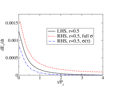
Figure 3: Numerical time derivative of the specific entropy of one representative equatorial tracer particle (left hand side of Eq. (IV.1)) for TMS evolution. Also, estimates of the expected heating rate (right hand sides of Eq. (IV.1)) using the exact covariant shear tensor and using the TMS closure $\tau_{ij}$ (Eq (54)).

As a first test of our momentum transport methods, we evolve a differentially rotating relativistic star. The initial equilibrium state is supplied by the code of Cook, Shapiro, and Teukolsky Cook et al. (1992). We use a polytropic equation of state $P=\kappa\rho_{0}^{\Gamma}$ with $\kappa=1$, $\Gamma=2$. The differential rotation law is

$$u^{t}u_{\phi}=R_{\rm eq}^{2}A^{2}(\Omega_{c}-\Omega)\,$$ (68)

where $R_{\rm eq}$ is the equatorial coordinate radius, $\Omega$ is the angular velocity, $\Omega_{c}$ is the angular velocity on the axis, and the differential rotation parameter $A$ is set to 1. The star has baryonic mass 0.1756$\kappa^{1/2}c^{2}G^{-3/2}$, ADM mass 0.1627$\kappa^{1/2}c^{2}G^{-3/2}$, and angular momentum 0.01402$c^{3}\kappa G^{-2}$. The polar to equatorial radius ratio is 0.75. The equatorial coordinate radius is 0.885$\kappa^{1/2}G^{-1/2}$.

We first evolve the star on a 2D grid assuming axisymmetry using the techniques described in our recent paper Jesse et al. (2020). We use a 2D Cartesian grid, with vertical and radial cylindrical polar coordinates $z$ and $\varpi$. We use $G=c=\kappa=1$ units. The grid has 360 points covering $-2\leq z\leq 2$ and 260 points covering $0<\varpi\leq 2.6$.

We set the viscous coefficient to $\eta=0.1P$, where $P$ is the pressure. For this test, we are uninterested in low density behaviors (e.g. winds), so we add an exponential suppression factor when $\rho_{0}$ is below $\rho_{\rm cut}=0.1\rho_{0\rm max}$, where $\rho_{0\rm max}$ is the initial maximum rest density: $\eta\rightarrow\eta e^{-(\rho_{\rm cut}/\rho_{0})^{4}}$. The driving timescale $t_{d}$ for $\sigma_{ij}$ is set to 0.12, much shorter than the initial central rotation period of 15.

In Figure 1, we plot the angular velocity profiles. For both the NS evolution and the TMS evolution, the rotation profile flattens inside the star, as expected. We do see that for the TMS evolution, the profile settles with a slight nonzero level in the high-density region. We pointed out in Section III.3 above that this would be a possibility, so its occurrence is not too surprising. Because it is not derived from the covariant stress tensor $\sigma$, the TMS stress $\tau$ can be zero when $\sigma$ is nonzero, and vice versa, for a general metric. Because it is coordinate-independent, the scalar $\sigma_{\alpha\beta}\sigma^{\alpha\beta}$, which we measure in the viscous heating tests below, is the most reliable measure of whether local shear is really present.

In Figures 2 and 3, we plot the heating rate of a representative tracer particle, plotting the left and right-hand sides of Eq. (IV.1). One could also plot the integrals of each side over the entire star, but then numerical error would be dominated by the thin numerically heated layer at the surface of the star. This heating is present even in the absence of TMS or NS transport and is mainly due to numerical viscosity, and thus is not expected to be directly related to the chosen subgrid viscosity model.

For the TMS evolution, we calculate $\sigma_{\alpha\beta}$ appearing in the heating rate (Eq. (IV.1)) in two ways. We compute the full covariant $\sigma_{\alpha\beta}$ that would appear in the Navier-Stokes equations (Eq. (II.2)). We also compute $\sigma_{\alpha\beta}$ from the closure $\tau_{ij}$ extended to 4-dimensions using $u^{\alpha}\sigma_{\alpha\beta}=0$. For the NS evolution, the agreement between local viscous heating rate and observed entropy increase is quite good, as it should be. The approach of the right-hand side to zero is particularly notable, since the shear scalar is an invariant measure of shear, and hence its disappearance of the approach to uniform rotation.

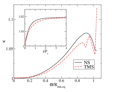
Figure 4: Entropy variable $\kappa=P/\rho_{0}^{\Gamma}$, where $\Gamma=2$, for NS and TMS runs. Main plot: The equatorial profile of $\kappa$ after 4 initial central rotation periods. Radii beyond the initial equatorial radius have low density and less accurate thermal evolution. Inset: Evolution of $\kappa$ for a representative equatorial tracer particle starting at around 0.6$R_{\rm eq,init}$.

For the TMS evolution, we see clearly that the effects of $\tau$ turn off while the covariant $\sigma$ is still nonzero, which we also noted in discussing the angular velocity evolution. However, the results again qualitatively match expectations. Fluid elements heat as angular momentum is transported outward. It should be emphasized that the disagreement between left and right-hand sides does not in itself indicate an error in the TMS method; neither of these right-hand sides is the exact entropy generation rate for the TMS stress; they only explain why viscous effects turn off while a small amount of invariant shear remains (because the $\tau$ stress has nearly vanished). In particular, it does not indicate that a deficit of heating is causing energy to disappear. Viscosity will tend to convert kinetic energy to heat; TMS in leaving residual shear may simply transfer slightly less energy without large violations of energy conservation. For self-gravitating systems, this analysis is complicated by changes in gravitational potential energy, and in general relativity total energy is only defined globally by the asymptotic metric. Unfortunately, our metric evolution is not accurate enough to study small changes in total energy that might arise from the TMS terms not coming from a covariant divergence of a 4D stress tensor. With our version of the energy equation, we are at least guaranteed energy conservation in the Newtonian limit.

To study the viscous heating further, Figure 4 compares the variable $\kappa=P/\rho_{0}^{\Gamma}$, a function of entropy initially equal to one throughout the star, for NS and TMS evolutions. The entropy at the final time is higher for the NS case. This is partly the effect of greater viscous heating, but when we look at heating at tracer particle locations (see the figure’s inset), we see that the heating of individual fluid elements is more similar for NS and TMS than the entropy profile would suggest. The reason is that the stellar interior expands a bit more in the TMS case than in the NS case, so that the tracked fluid elements end up at larger radii. To speak loosely, it is better to think of the TMS entropy profile as “shifted to the right” compared to the NS profile, rather than as “shifted down”. By tracking specific entropy rather than internal energy, we eliminate the effects of work energy expanding or compressing the fluid.

IV.2 Late-time three-dimensional evolution

We next evolve the star on a 3D grid to determine non-axisymmetric stability. In addition to the TMS and NS evolutions, we evolve the TMS with $k_{1}=k_{2}=0$ for equations (III.1) and (III.1). We let $\eta=0.05P$, and run the evolution to the viscous timescale to reach an equilibrium of constant angular momentum and heating.

Heating is measured by entropy generated, with entropy defined as

$$S=\rho_{*}\log\bigg{(}\frac{P}{\rho_{0}^{2}}\bigg{)}H\big{(}\rho-2\times 10^{-6}\kappa^{-1}c^{2}\big{)}$$ (69)

with $H$ being the Heaviside function, to cutoff unphysical entropy growth in the low density atmosphere.

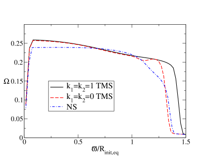
Figure 5: Azimuthally averaged angular velocity along equitorial radius at time $t=6.6P_{c}$.

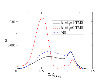
Figure 6: Azimuthally averaged entropy along equatorial radius at time $t=6.6P_{c}$.

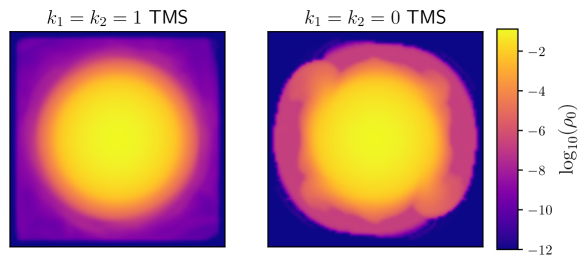
Figure 7: Snapshots of equatorial density at time $t=10.4P_{c}$ for TMS simulations with $k_{1}=k_{2}=1$ and $k_{1}=k_{2}=0$ in equations (III.1) and (III.1). The growth of the $L=4$ mode for $k_{1}=k_{2}=0$ is visible.

In figure  5, we can see similar behavior in the angular velocity as the axisymmetric evolution, with the TMS evolutions settling to a non-zero gradient. The $k_{1}=k_{2}=1$ TMS does show additional expansion of low density material, which is visible in the density comparison in figure 7.

The entropy in figure 6 shows a very similar behavior between the $k_{1}=k_{2}=1$ TMS and NS evolutions, as expected. In contrast, there is large difference in location and magnitude, of heating between the $k_{1}=k_{2}=0$ TMS and $k_{1}=k_{2}=1$ TMS evolutions, with additional localized heating closer to the core for the $k_{1}=k_{2}=0$ TMS evolution. The entropy peak of the $k_{1}=k_{2}=0$ does drift slowly outward as the simulation progesses.

When we implement the $k_{1}=k_{2}=0$ TMS method in SpEC, we observe a $L=4$ mode instability that results in unphysically strong winds and outflows of low density material. When the matter reaches the boundary, we are forced to terminate the simulation. With a domain size of 3.6$R_{\rm eq}$, we did convergence testing with 59, 74, 115, and 144 grid points. Increasing domain resolution does result in a delayed instability appearance time, but the growth timescale remains relatively constant for all resolutions, and is always slightly longer than the timescale needed to reach an equilibrium angular velocity profile in the star.

Recently, Nedora et al Nedora et al. (2019) have carried out binary neutron star merger simulations using Radice’s TMS transport. They find that spiral density waves in the postmerger remnant generate a wind that could cause a blue kilonova like that observed as the AT2017gfo counterpart to the binary neutron star merger event GW170817. Although the instability reported here may have been present in their simulations, and a comparison run with $k_{1}=k_{2}=1$ is recommended, it is very unlikely that this would significantly alter the conclusions of that paper. The existence of spiral waves in post-merger remnants is confirmed by prior purely hydrodynamical simulations Shibata and Uryū (2000); Shibata and Taniguchi (2006); Bernuzzi et al. (2014, 2016); Kastaun and Galeazzi (2015); Paschalidis et al. (2015); East et al. (2016); Lehner et al. (2016); Radice et al. (2016). Also, Nedora et al find that TMS transport only enhances the outflow mass by $\sim$25%.

V Tests on a Black Hole Accretion Torus System

The astrophysical system most commonly modeled using a phenomenological viscosity is, of course, disk accretion onto a star or compact object. For accretion to occur, angular momentum must be transported outward. It is, thus, important to study the behavior of different momentum transport treatments in an accretion disk system and note any major differences.

We evolve a Fishbone-Moncrief torus Fishbone and Moncrief (1976), for which $u^{t}u_{\phi}$ (roughly, the specific angular momentum) is constant, in our case set to 4.1$M$, where $M$ is the mass of the black hole. At the center is a black hole with dimensionless spin 0.9. The disk mass is assumed to be much smaller than that of the black hole, so the spacetime is set to the Kerr solution in Kerr-Schild coordinates and not evolved. The disk inner and outer initial radii are 4.5$M$ and 36$M$, respectively. The initial density maximum is at a ring of radius 10$M$. The gas of the disk is modeled with $\Gamma=4/3$ equation of state. The disk is initially isentropic and obeys a $\Gamma=4/3$ polytropic law. (Once evolution begins, the gas will heat.) All disk mass output below is scaled to the disk’s initial baryonic mass, which can therefore be taken to be one. This particular system is not designed to closely model any particular astrophysical scenario, although a high compaction of the disk (as measured by radius of maximum density divided by black hole mass) is chosen to be similar to tori encountered in binary post-merger simulations.

We evolve this system using both TMS (with $k_{1}=k_{2}=1$) and NS momentum transport using an alpha viscosity with $\alpha_{\rm visc}=0.03$. For TMS simulations, this corresponds to a mixing length

$$\ell=\alpha_{\rm visc}c_{s}/\Omega_{K}\ ,$$ (70)

with $\Omega_{K}$ the Keplerian angular velocity. Viscosity is suppressed by an exponential factor for density less than $10^{-4}$ of the initial maximum, and for gas at radii less than $3M$. We evolve on a 2D polar grid with 300 radial points and 256 angular points, uniformly spaced in the standard accretion grid variables

$$r =\sqrt{x^{2}+z^{2}}=e^{x_{1}},$$ (71)

$$\theta =\pi x_{2}+\frac{1}{2}(1-h)\sin(2\pi x_{2})\ ,$$ (72)

where for these simulations we use $h=0.5$. The grid covers the range $1.32M\leq r\leq 2000M$, $0<\theta<\pi$. A lower-resolution of $200\times 168$ gives similar results.

We evolve for 100,000$M$. This is long enough for the baryonic mass on the grid to drop to 20% of its initial value for the NS run, 10% for the TMS run. We terminate at this time because by this time the outer boundary is no longer sufficiently far. (This can be seen from the outflow. At earlier times, flow through the outer boundary is entirely unbound. Late in the evolution, the outgoing mass flux has unbound and weakly bound components, and by $t\approx 10^{5}M$, the latter has become comparable to the former.)

The baryonic mass flow rate into the black hole and out of the outer boundaries are plotted in figures 8 and 9. The flow rate into the black hole is seen to be fairly insensitive to the momentum transport method used. Over the evolved time, 50% of the baryonic mass accretes into the black hole in the TMS simulation, 60% in the NS simulation. While the difference is not negligible, few would expect any simple phenomenological model of subgrid turbulent momentum transport to be more accurate than a few tens of percent. At late times, the accretion rate falls off roughly like a power law $\dot{M}\propto t^{-n}$ where $1.7\leq n\leq 2$.

The outflow rates show rather larger differences, mostly because of a single large burst of unbound ejecta in the TMS simulation that is much smaller in the NS evolution. Over the evolved time, 17.6% of the original baryonic mass is ejected from the outer boundary in the NS evolution: 15.8% unbound and 1.8% bound. For the TMS evolution, 41.1% of the original baryonic mass leaves the outer boundary: 39.4% unbound and 1.7% bound. In fact, the slightly higher accretion rate into the black hole in the NS case might be mostly due to the larger mass remaining in the disk that did not suffer this one-time ejection.

As a check on whether these differences exceed numerical errors, we evolved the NS case at two other resolutions, with 0.7 times and 1.3 times the number of gridpoints in both radial and angular directions, and we use the differences between resolutions to estimate truncation error. Matter inflow into the black hole shows weak dependence on resolution, with errors of a few percent. The outflow mass is more difficult to resolve and may have error of almost 30%. We also reran TMS at the lower resolution and found a nearly 20% difference in outflow mass. Thus, the uncertainty in outflow measurements is tens of percent, which, while not ideal, is still significantly smaller than the difference between NS and TMS. We have also checked to see if our results are sensitive to the abruptness with which we begin to apply momentum transport. We perform an additional NS run in which the viscous parameter $\alpha_{\rm visc}$ is smoothly turned as $\alpha_{\rm visc}(t)=0.03(1-e^{-t/300})$. This leads to a 2% increase in accreted mass and roughly 10% decrease in outflow mass, so this effect also is dwarfed by the TMS-NS difference.

Of the two methods TMS involves fewer operations to take a timestep, but the NS runs are found to be about a factor of two faster because of the adaptive timestepping used by the SpEC code, which uses larger timesteps for NS runs to achieve the same time differencing accuracy.

Figures 8 and 10 show the effect of heat fluxes from entropy diffusion, using $\lambda_{S}=1$. The disk is initially isentropic, but viscous heating leads to higher entropy in the interior of the disk. Heat fluxes therefore supplement vertical convection and transport energy toward the top and bottom of the disk. The main effect of this is to increase the outflow through the outer boundary to 30.3% of the initial baryonic mass (28.7% of the initial disk mass in unbound outflow).

The production of unbound matter begins differently in simulations with vs. without heat fluxes. In both cases, there is very little unbound material for the first $\sim 2000M$. Without heat conduction, viscous heating produces a fairly distinct high-entropy region in the equator which advects inward. When it approaches the inner edge of the disk, it expands vertically, and the first large mass of unbound matter is ejected from the inner disk region in the polar direction. With heat conduction, the entropy entropy gradient remains smoother and shallower ($\kappa\equiv P/\rho_{0}^{\Gamma}$ is about a factor of two smaller at the equator than in runs without conduction). Heat transport is thus primarily by subgrid-scale convection rather than large-scale convection.  While a high-entropy region does advect inward at the same time as in the conduction-free simulations, the perturbation of the inner disk is far less violent, and only a small mass becomes unbound at this time. Instead, the massive outflow begins later and starts at the outer disk, leading to an equatorially concentrated initial burst. Longer simulations would be needed to determine if the angular distribution of the cumulative ejecta is very different depending on whether heat flux terms are included, but our test suggests that this could be a possibility in some cases.

Finally, we perform a demonstration of the possible effect of particle diffusion on the outflow composition. We introduce a composition variable $Y$ which is advected by the flow. Because it does not enter into the equation of state, it does not affect the evolution (except at the level of truncation error in the time discretization, if the evolution of $\rho Y$ is allowed to occasionally control the adaptive timestep). Ejecta composition is of great interest in post-merger simulations because of its connection to kilonovae and r-process nucleosynthesis. Since our simulation lacks neutrino interactions, it should be considered only a demonstration of another possibly significant influence.

We initialize $Y$ as

$$Y=\begin{cases}0.5-6\rho_{\rm 0,init}/\rho_{\rm 0,init,max},&\text{if }\rho_{\rm 0,init}/\rho_{\rm 0,init,max}<\frac{1}{15}\\ 0.1,&\text{otherwise}\end{cases}$$ (73)

The idea of using a simple analytic form with higher $Y$ at low densities and $Y=0.1$ at high densities was taken from Fujibayashi et al. (2020), which in term is a rough fit to the electron fraction in binary neutron star post-merger accretion disks. We evolve without particle diffusion ($\lambda_{D}=0$) and with it ($\lambda_{D}=$1). Both simulations use NS transport and compute the mean free path from $\alpha_{\rm visc}$ as in Eq. (70). We integrate the mass flux passing through the surface $r=800$M in $Y$ bins to get the total mass outflow as a function of $Y$, which is plotted in Fig. 11. In this example, the effect of particle diffusion is to shift the distribution peak to higher $Y$ and to make it narrower. One noticeable difference is that the high-$Y$ tail of the outflow distribution disappears when particle diffusion is added. Recall that in this simple test, the composition variable does not affect the equation of state and indeed plays no role in the hydrodynamics at all, so the same fluid elements are ejected in both simulations. However, there is a fairly strong $Y$ gradient in the initial disk near the low-density layers at the top and bottom edges of the disk, and this is where the high-$Y$ material is. The diffusion term causes the $Y$ composition variable to “bleed into” the disk, significantly lowering $Y$ near the surface of the disk. This flow of particles will also raise $Y$ in the disk interior, but the composition flux will lower $Y$ near the surface more than it will raise $Y$ in the interior, because the density is higher in the latter region.

Overall, the effect of smoothing the $Y$ distribution is that $Y$ does not vary as much in the density layers that provide the ejecta. Of course, the effect may be different for different composition distributions or in the presence of composition source terms (e.g. neutrino interactions). Interestingly, a detailed comparison of disks evolved with $\alpha$-viscosity vs magnetohydrodynamics found an opposite effect, that the MHD run had wider composition distribution at a lower peak Fernández et al. (2019). The diffusive effects of magnetorotational turbulence is certainly one effect present in MHD simulations but not viscous simulations without particle diffusion, although in this case outflows driven by large-scale magnetic fields may have been the more important difference.

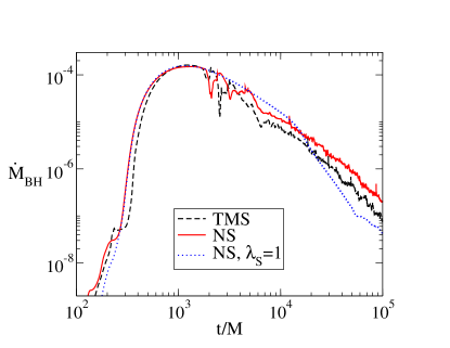
Figure 8: The accretion rate, defined as the fraction of the total baryonic mass of the disk accreted into the black hole per interval $M$ of time, for TMS, NS, and NS with turbulent heat flux.

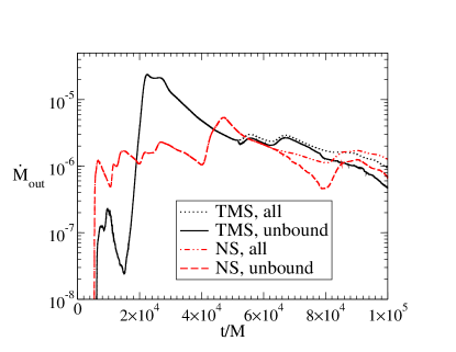
Figure 9: The outflow rate, defined as the fraction of the total baryonic mass of the disk leaving the outer boundary per interval $M$ of time, for TMS and NS runs. We plot separately the total outflow of mass and the outflow of unbound mass. Unbound matter is here defined as $u_{t}<-1$; defining it as $hu_{t}<-1$ has an insignificant effect on the unbound outgoing flux.

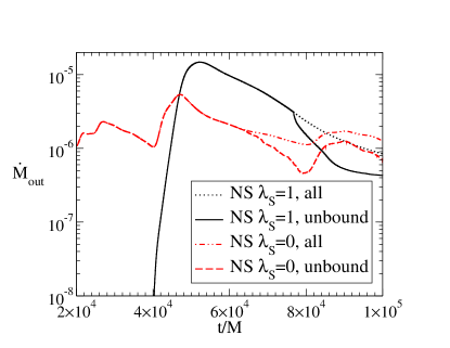
Figure 10: Outflow (total and unbound-only) for NS runs with and without turbulent heat conduction.

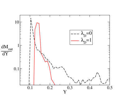
Figure 11: The distribution of composition variable $Y$. $\frac{dM}{dY}$ is defined such that the baryonic mass $dM_{0}$ within $dY$ of $Y$ is $dM_{0}=\frac{dM}{dY}dY$.

VI Conclusion

Even for a given choice of the effective viscosity $\eta$ there is some freedom in how one adds momentum transport to the relativistic Euler equations. In this manuscript, we perform detailed comparison of two models currently in use in numerical relativity simulations: Shibata el al’s NS model, and Radice’s TMS model. We also propose an improvement to the TMS model: the addition of physically motivated terms that guarantee that the stress-energy tensor remains a spatial tensor in the fluid rest frame, and prevents slowly-growing instability to appear in some test problems. The main objective of these models in merger simulations has been to provide angular momentum transport in the post-merger remnant. We find that the NS, original TMS, and modified TMS model fortunately behave very similarly in that respect, at least within the expected uncertainties of a mean field turbulence model. However, we find significant differences in viscous heating between the original TMS and the other two models, while all models provide different results for the momentum transport-driven ejecta mass in disk simulations. It is already known that disk outflow masses depend on $\alpha_{\rm visc}$. To this, we add that even if a “correct” $\alpha_{\rm visc}$ were known, outflows would still depend on the transport formalism.

As the TMS formalism is not 4-dimensionally covariant, its results might not apply for arbitrary foliations of the spacetime. We doubt, however, that the slicing choices usually used by numerical relativists would lead to dramatically different foliations, or that the gauge-dependence of TMS would impact numerical results more than the approximations inherent to any mean field model. Additionally, as the TMS model is simpler to implement and computationally less expensive than the NS model (at least on a per timestep basis), it certainly remains very useful to numerical simulations. The improvements to the TMS model proposed in this manuscript add new terms to the evolution equations, but without increasing the complexity of the evolution algorithm itself, or meaningfully impacting the cost of simulations. They should thus be reasonably simple to implement in any TMS-based code.

Mean-field models of subgrid transport effects provide an economical way to explore deep into the post-merger regime, although of course they cannot replace a more limited number of expensive high-resolution simulations. These models could easily be improved beyond what we have attempted here. An adequate model of subgrid effects would have to include heat transport, and it should also account for the effective pressure from turbulent stresses which has proved to be potentially quite important in the supernova core collapse problem Couch and Ott (2015). It would also be interesting to add the evolution of the large-scale magnetic field–even if the magnetorotational instability is subgrid scale– in order to incorporate large-scale magnetohydrodynamic effects such as magnetic braking and jet collimation. In the presence of subgrid turbulence, the induction equation for the mean magnetic field would itself need to be suitably augmented to include subgrid electromotive force terms, as is done in dynamo modeling Brandenburg and Subramanian (2005) and even in a few relativistic simulations Giacomazzo et al. (2015); Sadowski et al. (2015). If the mean field grows large enough to resolve the magnetorotational instability, then one would more correctly be in a regime for large eddy rather than mean field modeling.

One might question the point of improving models which at best capture their effects to no better than order of magnitude anyway. It is useful for at a couple of reasons. First, one is able to establish the sensitivity of particular outputs to various transport effects, as we have done with disk outflow composition, so that it is known what effects are most important for high-resolution simulations to capture. Second, these simplified models play an important role in interpreting high resolution results, guiding the inevitable tradeoff between exactness and human intelligibility.