Energy optimization of two-level quantum Otto machines

Abstract

We present the spin quantum Otto machine under different optimization criterion when function either as a heat engine or a refrigerator. We examine the optimal performance of the heat engine and refrigerator depending on their efficiency, output power and maximum entropy production. For heat engine case, we obtain the expression for the upper and lower bounds efficiencies at maximum power and maximum ecological function. In addition, the spin quantum Otto refrigerator coefficient of performance is optimized for three different criterion – cooling power, product of performance and power and ecological function. We further study the dimensionless power loss to the cold reservoir when the machine is operating as a heat engine as well as its counterpart for the refrigerator case. We find that the maximum operation of the heat engine (refrigerator) cycle is when optimized with respect to hot (cold) reservoir frequency.

I Introduction

Heat engines and refrigerators are two main classes of the thermal machines that are important in our daily life. Heat engine converts the heat energy into the mechanical work, while the refrigerator absorb the heat energy from the lower temperature bath and dump it into the higher temperature bath via the external work. Based on the second law of thermodynamics, the maximum efficiency of a traditional reversible and cyclic heat engine pioneered by Sadi Carnot is $\eta_{\text{C}}\!=\!1-T_{c}/T_{h}$, where $T_{c}$ and $T_{h}$ are temperatures of the cold and hot reservoir respectively Callen (1985). The refrigerator is functioning as heat engine inverse and the associated maximum coefficient of performance (COP) is $\epsilon_{C}\!=\!T_{c}/(T_{h}-T_{c})$ Callen (1985). However, the Carnot efficiency (COP) is reached only when the heat engine (refrigerator) is infinitely slowly operated to satisfy reversibility. For practical purposes in thermodynamics, engineering and biochemistry; it is important to understand the thermodynamics optimization of irreversible thermal machines for best performance/efficiency Andresen (2011).

In particular, for heat engines, the efficiency at maximum power has been studied extensively and mainly characterized by the Curzon-Ahlborn efficiency $\eta_{CA}\!=\!1-\sqrt{1-\eta_{C}}=\eta_{C}/2+\eta_{C}^{2}/8+\eta_{C}^{3}/16+5\eta_{C}^{4}/128+\mathcal{O}\left(\eta_{C}^{5}\right)$ Curzon and Ahlborn (1975); Esposito et al. (2010); Andresen (2011); Deffner (2018). Although, the maximum power maximization counterpart of refrigerator is not straightforward, the COP at maximum cooling power of low-dissipation refrigerators is $\epsilon^{\text{mp}}\!=\!\epsilon_{C}/(2+\epsilon_{C})$ Apertet et al. (2013); Holubec and Ye (2020). In addition, another meaningful figure of merit to characterize a refrigerator is the product of the COP and the cooling power of the refrigerator, the COP at maximum $\chi$ figure of merit, $\epsilon_{\text{YC}}\!=\!\sqrt{1+\epsilon_{C}}-1\!=\!\epsilon_{C}/2-\epsilon_{C}^{2}/8+\epsilon_{C}^{3}/16-5\epsilon_{C}^{4}/128+\mathcal{O}\left(\epsilon_{C}^{5}\right)$ Yan and Chen (1990); Chen et al. (2001); Abah and Lutz (2016). Besides the maximum efficiency and maximum power criteria, Angulo-Brown proposed the ecological optimization criterion of heat engines which take into account the trade-off between the high power output and the power loss due to entropy production, the Angulo-Brown efficiency $\eta_{AB}\!=\!3\eta_{C}/4+\eta_{C}^{2}/32+3\eta_{C}^{3}/128+37\eta_{C}^{4}/2048+\mathcal{O}\left(\eta_{C}^{5}\right)$ Angulo-Brown (1991); Ocampo-García et al. (2018).

Following the pioneering work of Scovil-Schulz-DuBois on a three-level maser heat engine Scovil and Schulz-DuBois (1959), there has been progress in the development of quantum thermal machines Bender et al. (2000); Humphrey et al. (2002); Lin and Chen (2004); Kosloff and Feldmann (2010); Abah et al. (2012); Harbola et al. (2012); Thomas et al. (2012); Goswami and Harbola (2013); Wang et al. (2013); Latifah and Purwanto (2013); Sutantyo et al. (2015); Hofer et al. (2016); Correa and Mehboudi (2016); Dattagupta and Chaturvedi (2017); Yin et al. (2017); Chand and Biswas (2017); Singh and Johal (2017); Newman et al. (2017); Roulet et al. (2018); Rojas-Gamboa et al. (2018); Hewgill et al. (2018); Oladimeji (2019); Singh and Johal (2019); Chattopadhyay and Paul (2019); Singh and Ram (2020); Singh (2020); Saputra and Ainiya (2020); Barontini and Paternostro (2019); Myers and Deffner (2020); Wiedmann et al. (2020); Peña et al. (2020). These studies have investigated quantum version of the most classical thermodynamics cycles, such as; Carnot, Otto, Diesel and Brayton. The working substances considered are two-level atomic system Wang et al. (2013), harmonic oscillator Abah et al. (2012); Newman et al. (2017), many-body systems Jaramillo et al. (2016), among others Latifah and Purwanto (2013); Sutantyo et al. (2015); Dattagupta and Chaturvedi (2017); Thomas et al. (2012, 2018); Hofer et al. (2016); Li et al. (2018). Moreover, recent time, there has been tremendous success in miniaturization of thermal engines Roßnagel et al. (2016); Josefsson et al. (2018); Van Horne et al. (2020) and refrigerator Maslennikov et al. (2019) down to nanoscale as well as those operating in quantum regime Klatzow et al. (2019); Peterson et al. (2019).

However, due to the increasing needs of energy consumption, resource availability, and environmental impact, the optimization of these real thermal engines/refrigerators are very desirable Long and Liu (2016); Açıkkalp and Ahmadi (2018). Hernandez et. al. put forward a unified criterion for energy converters that is laying between those of maximum efficiency and maximum useful energy Hernández et al. (2001). The ecological criterion for the heat engines is $E_{H}\!=\!\dot{W}-T_{c}\,\dot{S}_{\text{tot}}$ while for the refrigerator, it is $E_{R}\!=\!\dot{Q}_{\text{out}}-\epsilon_{C}T_{h}\dot{S}_{\text{tot}}$, where the dot (hereafter) is the time derivative with respect to the total cycle time, $W$ is the total work done, $Q_{\text{out}}$ is the heat output, and $S_{\text{tot}}$ is the total entropy production Hernández et al. (2001).

In this work we study the optimal performance of the two-level Otto engine/refrigerator from the viewpoint of the efficiency, power and entropy production. This model of the spin quantum heat engine is recently implemented using the nuclear magnetic resonance setup Peterson et al. (2019). Moreover, we study the power associated with optimal performance of the Otto cycle at different type of optimizations. Then, calculated the fractional power lost/dump of the engine/refrigerator cycle due to the entropy production.

The remainder of the paper is organized as follows. In section II we present the two-level atomic system thermodynamic quantities and the Otto cycle model. In Section III we present the analysis of Otto cycle when functioning as a heat engine. Then, the optimal efficiencies are computed for two different optimization criterions, namely the efficiency at maximum power (Section III.1) and ecological function (Section III.2). We examine the refrigerator performance of Otto cycle for three different optimization in Section IV and in Section V we present our conclusions.

II Thermodynamics of two-level quantum Otto cycle

Let first discuss the thermodynamics of a quantum system. The average internal energy of a quantum system with discrete energy levels is $U\!=\!\sum_{n}E_{n}p_{n}$ where $E_{n}$ are the energy of the $n$-state/level and $p_{n}$ are the corresponding occupation probabilities. From an infinitesimally change in energy

$$dU=\sum_{n}(E_{n}dp_{n}+p_{n}dE_{n})$$ (1)

we can distinguish the infinitesimal work done $dW\!=\!\sum_{n}dE_{n}p_{n}$ and the heat $dQ\!=\!\sum_{n}E_{n}dp_{n}$. Thus, Eq. (1) can be seen as an expression of the first law of thermodynamics, $dU\!=\!dQ+dW$.

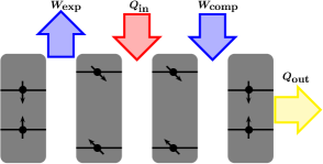
Figure 1: Schematic of a quantum Otto cycle constructed from the two-level system. The thermodynamic cycle consists of two adiabatic processes ($W_{\text{exp}}$ and $W_{\text{comp}}$) and two isochoric processes ($Q_{\text{in}}$ and $Q_{\text{out}}$).

We now consider a quantum Otto cycle whose working substance is a two-level system Lin and Chen (2004); Kosloff and Feldmann (2010); Abah et al. (2012); Kosloff and Rezek (2017); Peña et al. (2020), see the pictorial representation in the Fig. (1). Specifically, for a two-level system described by the Hamiltonian $H\!=\!-\hbar\omega_{t}\sigma_{z}$, where $\hbar$ is the Planck constant, $\omega_{t}$ is the external controlled angular frequency and $\sigma_{z}$ is the $z$-component Pauli matrix. The associated occupation probabilities are given by $p^{i}_{\pm}\!=\!\exp(\pm\beta_{i}\hbar\omega_{i})/Z_{i}$ and the partition function is $Z\!=\!\exp(\beta\hbar\omega_{i})+\exp(-\beta_{i}\hbar\omega_{i})$, where $i=c/h$ denotes the low/high angular frequency, $\beta_{i}=1/k_{\text{B}}T_{i}$ is the inverse temperature and $k_{\text{B}}$ is the Boltzmann constant. The Otto cycle consists of two adiabatic branches where the external field $\omega_{t}$ varies with its energy-level structure and the two isochoric branches describes the working medium in contact with the cold/hot bath at constant control field $\omega$. The four-stroke stages of the cycle are ($\hbar\!=\!1$);
(i) adiabatic expansion – the two-level system initially prepared at frequency $\omega_{c}$ undergoes a unitary evolution to reach a higher angular frequency $\omega_{h}>\omega_{c}$. The occupation probabilities for the two states remain unchanged according to the quantum adiabatic theorem Messiah (1999). The work done during the expansion is given as

$$W_{\text{exp}}=p_{+}^{c}(\omega_{h}-\omega_{c})-p_{-}^{c}(\omega_{h}-\omega_{c}).$$ (2)

(ii) isochoric heating – in this stage, the quantum system is coupled to the equilibrium hot thermal bath until it reaches the steady state at a constant angular frequency $\omega_{h}$. The work done during this process is zero and the corresponding heat input is given as

$$Q_{\text{in}} = -(\omega_{h}(p^{h}_{+}-p^{c}_{-})-\omega_{h}(p^{h}_{-}-p^{c}_{-})),$$

$$Q_{\text{in}} = \omega_{h}\left(\tanh\left(\beta_{c}\omega_{c}\right)-\tanh\left(\beta_{h}\omega_{h}\right)\right).$$ (3)

(iii) adiabatic compression – the quantum system is isolated and the frequency varied from $\omega_{h}$ to $\omega_{c}$ at constant occupation probability. Similar to the expansion stage, no heat is added and the work done during the adiabatic compression is

$$W_{\text{comp}}=p_{+}^{h}(\omega_{c}-\omega_{h})-p_{-}^{h}(\omega_{c}-\omega_{h}).$$ (4)

(iv) isochoric cooling step – the two-level quantum system is coupled to the cold thermal bath temperature characterized by $\beta_{c}$. The amount of heat discarded by the quantum system during this thermalization process reads

$$Q_{\text{out}} = -\left(\omega_{c}\left(p^{c}_{+}-p^{h}_{+}\right)-\omega_{c}\left(p^{c}_{-}-p^{h}_{-}\right)\right),$$ (5)

$$= -\omega_{c}\left(\tanh\left(\beta_{c}\omega_{c}\right)-\tanh\left(\beta_{h}\omega_{h}\right)\right).$$

For a complete cycle, the total work done becomes

$$W = -(W_{\text{exp}}+W_{\text{comp}})$$ (6)

$$= -\left(\omega_{h}-\omega_{c}\right)\left[\tanh\left(\beta_{c}\omega_{c}\right)-\tanh\left(\beta_{h}\omega_{h}\right)\right].$$

Thus, based on the first law of thermodynamics the amount of work $W$ produced by the engine or required by the refrigerator for any given cycle is

$$W=-(Q_{c}+Q_{h}).$$ (7)

In addition, an upper bound to the machine (engine/refrigerator) performance follows from the second law of thermodynamics, which states that the total entropy production of a cyclic thermal device is non-negative,

$$S_{\text{tot}}=-\beta_{h}Q_{h}-\beta_{c}Q_{c}.$$ (8)

In high-temperature limit, the total work done and heat input/output for a cycle can be written as

$$W = -\left(\omega_{h}-\omega_{c}\right)\left(\beta_{c}\omega_{c}-\beta_{h}\omega_{h}\right),$$ (9)

$$Q_{\text{in}} = \omega_{h}\left(\beta_{c}\omega_{c}-\beta_{h}\omega_{h}\right),$$ (10)

$$Q_{\text{out}} = -\omega_{c}\left(\beta_{c}\omega_{c}-\beta_{h}\omega_{h}\right).$$ (11)

In the rest of the paper, without lost generality, we will focus on the Otto cycle/machine operation at high-temperature limit.

III Two-level Otto heat engine

In this section, we will analyze the optimal performance of the two-level Otto heat engine using two different type of optimizations – efficiency at maximum power and ecological function. Moreover, we study their fractional power loss and compare their maximum output power. For the cycle to function as heat engine, the total work done $W>0$. The efficiency of the quantum Otto heat engine is

$$\eta_{O}=-\frac{W}{Q_{\text{in}}}=1-\frac{\omega_{c}}{\omega_{h}}.$$ (12)

The engine efficiency depends on their initial and final frequencies. Based on the positivity of the total work done, $W\geq 0$ which leads to the bound $1\leq\omega_{h}/\omega_{c}\leq\beta_{c}/\beta_{h}$, that is $\eta_{C}\!\geq\!\eta_{O}$. Alternatively, combining Eqs. (7) and (8), $\eta_{C}\!\geq\!\eta_{O}$. However, the maximum efficiency corresponds to zero output power, $P$ (i.e. total work done, $W$ per cycle time $\tau$) and occur when $\omega_{c}/\omega_{h}\!=\!T_{c}/T_{h}$.

III.1 Efficiency at maximum power

Now we will optimize the power output of the heat engine cycle with respect to $\omega_{h}$ for fixed temperatures, cold frequency $\omega_{c}$ and cycle time. The resulting optimal frequency ratio, $\omega_{c}/\omega_{h}\!=\!2\beta_{h}/(\beta_{c}+\beta_{h})$ with the corresponding efficiency and power are;

$$\eta_{\omega_{h}}^{\ast} = \frac{\eta_{C}}{2-\eta_{C}}$$ (13)

$$P_{\omega_{h}}^{\ast} = \frac{\beta_{c}\omega_{c}^{2}\eta_{C}^{2}}{4(1-\eta_{C})\tau}.$$ (14)

Expanding the efficiency in terms of $\eta_{C}$, we have

$$\eta_{\omega_{h}}^{\ast}=\frac{\eta_{C}}{2}+\frac{\eta_{C}^{2}}{4}+\frac{\eta_{C}^{3}}{8}+\frac{\eta_{C}^{4}}{16}+\mathcal{O}\left(\eta_{C}^{5}\right).$$ (15)

The smaller values of the $\eta_{C}$, the first term of Eq. 15 equals the $\eta_{\text{CA}}$ and it is plotted in Fig. 2. We observe that increasing values of $\eta_{C}$ gives optimal efficiency greater than the $\eta_{\text{CA}}$. At this point, it is worthy to mention that the high-temperature limit efficiency at maximum power of a harmonic oscillator working medium is $\eta_{\text{CA}}$ Abah et al. (2012).

On the other hand, when we optimize the power output with respect to $\omega_{c}$ at fixed temperatures, $\omega_{h}$ and cycle time, the optimal frequency ratio is $\omega_{c}/\omega_{h}\!=\!(\beta_{c}+\beta_{h})/2\beta_{c}$. The corresponding efficiency and power are

$$\eta^{\ast}_{\omega_{c}} = \eta_{C}/2,$$ (16)

$$P^{\ast} = \frac{\beta_{c}\,\eta_{C}^{2}\,\omega_{h}^{2}}{4\,\tau}.$$ (17)

Equation (16) matches with the first term of $\eta_{\text{CA}}$ and illustrated in Fig. 2. In general, the efficiency at maximum power is bounded as; $\eta^{\ast}_{\omega_{c}}\leq\eta^{\ast}\leq\eta^{\ast}_{\omega_{h}}$. We also note that the present results almost agree well with the CA efficiency even for $\eta_{C}$ up to 0.3, at which the evident deviation of the present result from the CA efficiency starts to appear.

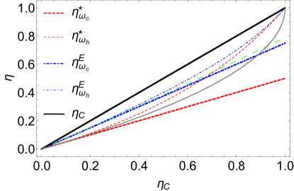
Figure 2: The Otto engine efficiency as a function of Carnot efficiency. The red (dashed) line is the efficiency at maximum work when optimized with $\omega_{c}$ (Eq. 16) while the red (light-dashed) line correspond to optimizing with $\omega_{h}$ (Eq. 13). The blue (dotted dashed) line shows the efficiency at $\omega_{c}$ maximum ecological function (Eq. 22) while the blue (light-dotted dashed) line is when the ecological function optimize with $\omega_{h}$ (Eq. 19). The black solid line is the Carnot efficiency $\eta_{C}$, the gray light solid line is the Curzon-Alhborn efficiency $\eta_{CA}$, while the green dashing line is the Angulo-Brown efficiency $\eta_{AB}$.

III.2 Efficiency at maximum ecological function

Let us consider the optimization of efficiency based on the ecological function with respect to the frequencies. In fixed cycle time, the ecological function defined as $E_{H}\!=\!\dot{W}-T_{c}\,\dot{S}_{\text{tot}}$ Hernández et al. (2001), in high-temperature limit reads

$$E_{H}\!=\!-\left(\beta_{c}\omega_{c}-\beta_{h}\omega_{h}\right)\left(\omega_{h}\eta_{C}-2\omega_{h}+2\omega_{c}\right).$$ (18)

We now optimize the ecological function, Eq. (18), with respect to $\omega_{h}$ to obtain the optimal frequency ratio as $\omega_{c}/\omega_{h}\!=\!2\beta_{h}(\eta_{C}-2)/(\beta_{c}(\eta_{C}-2)-2\beta_{h})$. The corresponding efficiency and power reads

$$\eta_{\omega_{h}}^{E} = \frac{\eta_{C}\left(2\eta_{C}-3\right)}{3\eta_{C}-4},$$ (19)

$$P_{\omega_{h}}^{E} = \frac{3\beta_{c}\,\omega_{c}^{2}\,\eta_{C}^{2}\left(2\eta_{c}+1\right)}{4\,\tau\left(\eta_{C}+2\right)^{2}\left(\eta_{C}-1\right)}.$$ (20)

The expansion of the efficiency (Eq. 19) is

$$\eta_{\omega_{h}}^{E}=\frac{3\eta_{C}}{4}+\frac{\eta_{C}^{2}}{16}+\frac{3\eta_{C}^{3}}{64}+\frac{9\eta_{C}^{4}}{256}+\mathcal{O}\left(\eta_{C}^{5}\right).$$ (21)

From Eq. (21), the first term is the same with the Angulo-Brown efficiency $\eta_{AB}$. It means that the for the small values of the $\eta_{C}$, both efficiencies match with each other as illustrated in Fig. 2.

Then optimizing the ecological function with respect to $\omega_{c}$, the resulting optimal frequency ratio $\omega_{c}/\omega_{h}\!=\!\left[\beta_{c}\,(1-\eta_{C}/2)+\beta_{h}\right]/2\beta_{c}$. The corresponding efficiency and power are

$$\eta_{\omega_{c}}^{E} = \frac{3\eta_{C}}{4},$$ (22)

$$P_{\omega_{c}}^{E} = \frac{3\beta_{c}\,\eta_{C}^{2}\,\omega_{h}^{2}}{16\,\tau}.$$ (23)

From the Fig. 2, we can see that the efficiency at maximum ecological function is higher than the efficiency at maximum power. The optimization with the $\omega_{h}$ gives the better results than the $\omega_{c}$. At the lower values of the $\eta_{C}$, the both efficiencies at the the maximum ecological function matches with the Angulo-Brown efficiency $\eta_{AB}$, while both the efficiencies at maximum power matches with the Curzon-Ahlborn efficiency $\eta_{CA}$. Likewise, the efficiency at maximum ecological function is bounded as; $\eta^{E}_{\omega_{c}}\leq\eta^{E}\leq\eta^{E}_{\omega_{h}}$. We remark that the resulting power for the optimization of maximum power and ecological function with respect to $\omega_{h}$ is the same for $\beta_{c}\!=\!\omega_{c}\!=\!1$ while $P^{\ast}_{\omega_{c}}\geq P^{E}_{\omega_{c}}$ for $\beta_{c}\!=\!\omega_{h}\!=\!1$.

III.3 Fractional power loss

To better understand the different between the two efficiency optimization criterion in the Sections. III.1 and III.2, we evaluate the ratio of power loss due to total entropy production (total entropy per unit time) to actual power output. Defining the power lost in terms of entropy production reads $P_{\text{lost}}\!=\!T_{c}\dot{S}_{\text{tot}}$ Angulo-Brown (1991), where $\dot{S}_{\text{tot}}\!=-\!\dot{Q}_{c}/T_{c}-\dot{Q}_{h}/T_{h}$. Using the definition of power $P\!=\!-\dot{W}\!=\!\dot{Q}_{\text{in}}+\dot{Q}_{\text{out}}$ and the efficiency $\eta\!=\!-W/Q_{\text{in}}\!=\!P/\dot{Q}_{\text{in}}$, the power loss reads

$$P_{\text{loss}}=\frac{P}{\eta}\left(\eta_{C}-\eta\right).$$ (24)

Thus, the ratio of power loss to maximum power output can be written as

$$R=\frac{P_{\text{loss}}}{P}=\left(\frac{\eta_{C}}{\eta_{\text{max}}}-1\right).$$ (25)

Equation (25) quantifies the lost associated with the maximum efficiency $\eta_{\text{max}}$ for any optimization criterion.

For the case of power optimization with respect to $\omega_{h}$, the fractional power loss for maximum power and ecological function respectively are

$$R_{\omega_{h}}^{\ast}\!=\!1-\eta_{C},\hskip 28.45274ptR_{\omega_{h}}^{EF}\!=\!\frac{\eta_{C}-1}{2\eta_{C}-3}.$$ (26)

Similarly, the optimization of power with respect to $\omega_{c}$, we have

$$R_{\omega_{c}}^{\ast}\!=\!1,\hskip 28.45274ptR_{\omega_{c}}^{EF}\!=\!1/3.$$ (27)

Figure 3 illustrate the fractional power loss as a function of temperature. We observe that the fractional power loss remains constant for optimization with $\omega_{c}$, while it decreases with $\eta_{C}$, when optimized with $\omega_{h}$.

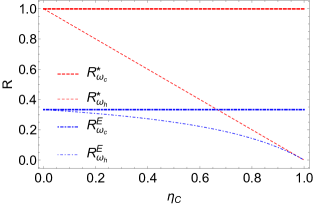
Figure 3: The dimensionless power loss with environmental temperature as a function of Carnot efficiency for different optimizations. The red (dashed) line corresponds to the maximum power optimization while the blue (dotted dashed) is the ecological function optimization.

In addition, the ratio of the heat engine maximum power and the power associated to maximum ecological function when optimised with $\omega_{h}$ reads $P^{\ast}_{\omega_{h}}/P^{E}_{\omega_{h}}\!=\!(\eta_{C}-2)^{2}/(3-2\eta_{C})$. On the other hand, the ratio when optimised with respect to $\omega_{c}$ is constant, i.e $P^{\ast}_{\omega_{c}}/P^{E}_{\omega_{c}}\!=\!4/3$. Thus, it is clear that the ratio remains constant, when it is optimized with the $\omega_{c}$, while the ratio decreases as we increase the $\eta_{C}$, when we optimize it with $\omega_{h}$

IV Two-level Otto refrigerator

Here, we present the analysis of the optimal performance of two level Otto refrigerator for two different optimizations. The main purpose of a refrigerator is to extract maximum possible of heat from the cold bath by performing a minimum amount of work.The Otto refrigerator coefficient of performance (COP) is defined as the ratio of output heat $Q_{\text{out}}$ to the total work done $W$ per cycle,

$$\epsilon_{\text{O}}=\frac{Q_{\text{out}}}{W}=\frac{\omega_{1}}{\omega_{2}-\omega_{1}}.$$ (28)

An Otto cycle functions as a refrigerator when the output heat is greater than zero. Based on the total entropy production for one complete cycle and the first law of thermodynamics, it can easily be shown that $\epsilon_{\text{O}}\!\leq\!\epsilon_{\text{C}}$. Another important quantity describing a refrigerator is cooling power, $P_{c}$, defined as heat extracted from the cold bath per cycle over the cycle duration,

$$P_{c}=Q_{\text{out}}/\tau.$$ (29)

For practical interest, we always have to find a compromise between cooling power and COP. However, it has been known that the optimization of refrigerator at maximum cooling power does not result to counterpart of efficiency at maximum power Apertet et al. (2013). Tomás et. al. proposed a unified optimization figure of merit as product of COP and cooling power of a refrigerator de Tomás et al. (2012). In what follows, we study refrigerator performance for three different optimization criterion.

IV.1 Optimization of the cooling power

Here, we find the maximum COP for a given cooling power. Maximizing the cooling power at constant cycle time with respect to $\omega_{c}$ gives the optimal cold frequency $\omega^{\ast}\!=\!\beta_{h}\omega_{h}/2\beta_{c}$ and the corresponding performance quantities as,

$$\epsilon^{\text{mp}}\! = \!\frac{\epsilon_{c}}{2+\epsilon_{c}},\hskip 28.45274pt$$ (30)

$$P_{c}^{\text{mp}}\! = \!\frac{\beta_{h}\epsilon_{\text{C}}\omega_{h}^{2}}{4\tau(1+\epsilon_{\text{C}})}.$$ (31)

The Taylor’s expansion of the COP is

$$\epsilon^{\text{mp}}\!=\!\frac{\epsilon_{c}}{2}-\frac{\epsilon_{c}^{2}}{4}+\frac{\epsilon_{c}^{3}}{8}-\frac{\epsilon_{c}^{4}}{16}+\mathcal{O}\left(\epsilon_{c}^{5}\right)$$ (32)

The $\epsilon^{\text{mp}}$, Eq. (30), is the same as the result obtained recently for Carnot-type low-dissipation refrigerators in the reversible limit Apertet et al. (2013); Holubec and Ye (2020). We see that the lower values of performance at the maximum cooling power is similar to the result of Yan-Chen Yan and Chen (1990); Chen et al. (2001). We remark that optimization with respect to $\omega_{h}$ leads to no physical results.

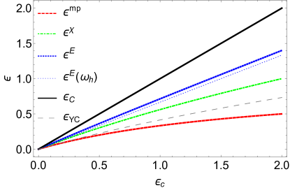
Figure 4: Coefficient of performance at different maximum optimization for the Otto refrigeration cycle as a function of the Carnot coefficient of performance $\epsilon_{\text{C}}$. The red (dashed) line shows the maximum cooling power case (Eq. 30), the green (dotted-dashed) line shows the $\chi$ figure of merit case (Eq. 34), the blue (dotted) line shows the ecological function case (Eq. 38) when maximised with $\omega_{c}$, while the blue (dotted) tiny line is when ecological function is maximised with respect to $\omega_{h}$. The black solid line is the Carnot coefficient of performance while the gray (large dashing) line is the Yan-Chen coefficient of performance, $\epsilon_{\text{YC}}$.

IV.2 Performance at maximum $\chi$ figure of merit

Now let consider the unified figure of merit $\chi\!=\!\epsilon\,Q_{\text{out}}/\tau$ defined as the product of the coefficient of performance $\epsilon$ and the cooling power of the refrigerator de Tomás et al. (2012); Abah and Lutz (2016). Optimizing the $\chi$ with respect to $\omega_{c}$ in the high-temperature limit gives the optimal frequency ratio,

$$\frac{\omega_{c}}{\omega_{h}}\!=\!\frac{-\sqrt{9\beta_{c}^{2}-10\beta_{c}\beta_{h}+\beta_{h}^{2}}+3\beta_{c}+\beta_{h}}{4\beta_{c}}.$$ (33)

The associated COP at maximum $\chi$ and cooling power are;

$$\epsilon^{\chi}\!=\!1/2(-3+\sqrt{(9+8\epsilon_{\text{C}})}),$$ (34)

$$P_{c}^{\chi}\!=\!\beta_{h}\frac{\left[(3+2\epsilon_{\text{C}})\sqrt{9+8\epsilon_{\text{C}}}-(9+10\epsilon_{\text{C}})\right]\omega_{h}^{2}}{8\tau\epsilon_{\text{C}}(1+\epsilon_{\text{C}})}.$$ (35)

Similar to optimization at maximum cooling power, the COP can be express in the form of Yan-Chen COP Yan and Chen (1990).

IV.3 COP at maximum ecological function

We now evaluate the COP at maximum ecological function, $E_{R}\!=\!\dot{Q}_{\text{out}}-\epsilon_{C}T_{h}\dot{S}_{\text{tot}}$. The ecological function of the two-level Otto refrigeration cycle in high temperature limit becomes

$$E_{R}=\frac{\left(\beta_{h}\omega_{h}-\beta_{c}\omega_{c}\right)\left(\beta_{c}\omega_{c}\epsilon_{\text{C}}+\beta_{h}\left(\omega_{c}-\omega_{h}\epsilon_{\text{C}}\right)\right)}{\beta_{h}}.$$ (36)

First, optimizing the ecological function of the Otto refrigerator with respect to $\omega_{h}$ at fixed temperatures, $\omega_{c}$ and cycle time, we have $\omega_{h}\!=\!(\beta_{h}\omega_{c}+2\beta_{c}\omega_{c}\epsilon_{\text{C}})/(2\beta_{h}\epsilon_{\text{C}})$ and the resulting COP and cooling power are

$$\epsilon_{\omega_{h}}^{E}=2\epsilon_{\text{C}}/3,\hskip 28.45274ptP_{c}^{E}(\omega_{h})=\frac{\beta_{h}\omega_{c}^{2}}{2\tau\epsilon_{\text{C}}}.$$ (37)

Alternatively, optimizing with respect to $\omega_{c}$, the optimal frequency $\omega_{c}\!=\!\beta_{h}\omega_{h}\left(\beta_{h}+2\beta_{c}\epsilon_{C}\right)/(2\beta_{c}\left(\beta_{h}+\beta_{c}\epsilon_{C}\right))$ with the COP at maximum ecological function and cooling power read

$$\epsilon^{E}(\omega_{c})\! = \!\frac{\epsilon_{\text{C}}\left(2\epsilon_{\text{C}}+3\right)}{3\epsilon_{\text{C}}+4},\hskip 8.5359pt$$ (38)

$$P_{c}^{E}(\omega_{c})\! = \!\frac{\beta_{h}\epsilon_{\text{C}}(2\epsilon_{\text{C}}+3)\omega_{h}^{2}}{4\tau(\epsilon_{\text{C}}+1)(\epsilon_{\text{C}}+2)^{2}}.$$ (39)

We remark that the resulting COP for maximization with respect to $\omega_{c}$, $\epsilon^{E}(\omega_{c})$ is slightly greater than $\epsilon_{\omega_{h}}^{E}$.

Figure 4 shows the COP at maximum cooling power (Eq. 30, red dashed line), the COP at maximum $\chi$ figure of merit (Eq. 34, green dotted dashed line) and COP at ecological function maximization (Eq. 38, blue dotted line). We observe that the COP all concides for large temperature difference (small $\epsilon_{\text{C}}$). The COP at maximum ecological function and the $\chi$ figure of merit are greater than the Yan-Chen COP, $\epsilon_{YC}$. Thus, the COP are related as; $\epsilon_{\text{C}}^{\text{mp}}\leq\epsilon_{\text{C}}^{\chi}\leq\epsilon_{\text{C}}^{E}$. In Fig. 5, we present the corresponding maximum cooling power for the different optimization. Their behaviour is inversely related to the maximum COP illustrated in Fig. 4.

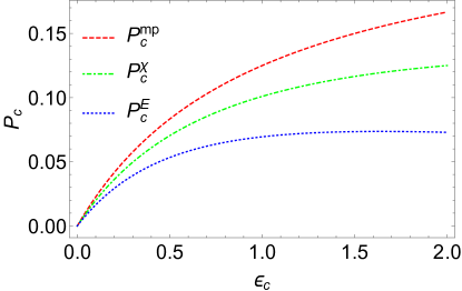
Figure 5: Cooling power at different maximum optimization for the Otto refrigeration cycle as a function of the Carnot coefficient of performance $\epsilon_{\text{C}}$. The red (dashed) line shows the maximum cooling power case (Eq. 31), the green (dotted-dashed) line shows the $\chi$ figure of merit case (Eq. 35), while the blue (dotted) line shows the ecological function case (Eq. 39) when maximised with $\omega_{c}$. The cooling power is in the unit $\beta_{h}\omega_{h}/\tau$.

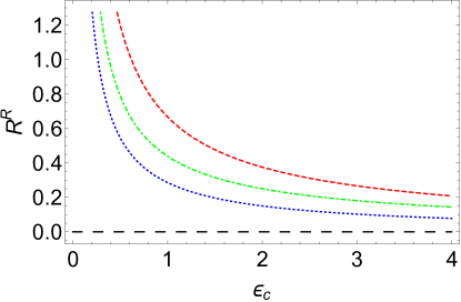
Figure 6: The fractional cooling power loss at different optimization as function of Carnot coefficient of performance. The red (dashed) line shows the maximum cooling power case (Eq. 44), the green (dotted-dashed) line shows the $\chi$ figure of merit case (Eq. 45), while the blue (dotted) line shows the ecological function case (Eq. 46). The large dashed black line is a guide to the eyes on point zero.

IV.4 Fractional cooling power dump

Here, in analogy to the fractional power loss of heat engine, we consider the dimensionless cooling power dump during a complete refrigeration cycle. Let us define the power dump due to the entropy generation in the hot reservoir as

$$P^{R}_{\text{dump}}\!=\!T_{h}\Delta\dot{S}_{\text{tot}}=T_{h}\left[-\frac{\dot{Q}_{h}}{T_{h}}-\frac{\dot{Q}_{c}}{T_{c}}\right],$$ (40)

where the environment temperature is equal to the hot temperature.

Employing the definitions, Carnot COP $\epsilon_{C}\!=\!T_{c}/(T_{h}-T_{c})\!=\!\beta_{h}/(\beta_{c}-\beta_{h})$ and Otto COP $\epsilon\!=\!Q_{c}/W$, we get

$$P^{R}_{\text{dump}}=\dot{Q}_{c}\left[\frac{1}{\epsilon}-\frac{1}{\epsilon_{C}}\right].$$ (41)

Thus, the dimensionless cooling power of any Otto refrigerator becomes

$$\mathcal{R}^{R}=\frac{P^{R}_{\text{dump}}}{P}=\left[\frac{1}{\epsilon}-\frac{1}{\epsilon_{C}}\right].$$ (42)

In the first order approximation of $\epsilon_{C}$, Eq. (42) can be re-written as

$$\mathcal{R}^{R}=\frac{1}{\epsilon_{C}^{2}}\left(\epsilon_{C}-\epsilon_{\text{max}}\right).$$ (43)

where $\epsilon_{\text{max}}$ is the resulting COP for a given optimization criterion. Thus, the cooling power loss associated with the COP at maximum cooling power, $\chi$ figure of merit and the ecological function when optimized with $\omega_{c}$ respectively are;

$$\mathcal{R}^{R}(mp) = \frac{1+\epsilon_{\text{C}}}{2\epsilon_{C}+\epsilon_{C}^{2}},$$ (44)

$$\mathcal{P}^{R}(\chi) = \frac{3+2\epsilon_{C}-\sqrt{9+8\,\epsilon_{C}}}{2\epsilon_{C}^{2}},$$ (45)

$$\mathcal{R}^{R}(E) = \frac{1+\epsilon_{\text{C}}}{4\epsilon_{C}+3\epsilon_{\text{C}}^{2}}.$$ (46)

Figure 6 present the dimensionless cooling power loss as a function of Carnot COP for different optimization protocol. It is clear that the power loss decreases as we increase the $\epsilon_{\text{C}}$ and the case of maximum ecological function gives lowest fractional power loss. In addition, the ecological function optimization with respect to $\omega_{h}$ yields a dimensional cooling power loss $\mathcal{R}^{R}(E_{\omega_{h}})\!=\!1/(3\,\epsilon_{C})$ that is higher than $\mathcal{R}^{R}(E)$ but the same in high values of $\epsilon_{\text{C}}$.

V Conclusion

We have studied the quantum Otto cycle whose working medium is a two-level system, first when functioning as a heat engine and later as a refrigerator. For one complete cycle, the two-level system alternate between two (hot and cold) thermal reservoirs by varying their angular frequency from $\omega_{c}$ to $\omega_{h}$. For heat engine, we analyze the optimal efficiency at maximum power as well as ecological function and find that the optimal efficiency at maximum ecological function is always greater than the maximum power case. Then, optimizing with respect to $\omega_{h}$ yields more efficiency than the case of $\omega_{c}$ for a particular optimization. In addition, we calculated the dimensionless power loss to the cold environment due to change in entropy per unit time and observe that while the optimization with respect to $\omega_{c}$ is constant, the optimization with $\omega_{h}$ depends on Carnot efficiency $\eta_{C}$. Moreover, the amount of power loss to environment is minimal for the case of ecological function than the maximum power.

On the other hand, we have studied the performance of Otto refrigeration cycle for optimal cooling power, $\chi$-function figure of merit and ecological function. The ecological function optimization gives highest COP while the cooling power optimization leads to the lowest values. However, the amount of power dump into the hot environment which decreases with the COP is more for the maximum cooling power than the ecological function scenario and always finite. Finally, we conclude that the heat engine cycle remains more beneficial when it is optimized with the $\omega_{h}$, while refrigeration cycle remains more beneficial when it is optimized with the $\omega_{c}$.

VI Acknowledgement

We are thankful to Colin Benjamin and Varinder Singh for their valuable comments. OA acknowledge the support by the Royal Commission for the Exhibition of 1851.

References

- Callen (1985) H. Callen, Thermodynamics and an Introduction to Thermostatistics (Wiley, New York, 1985).
- Andresen (2011) B. Andresen, Angewandte Chemie International Edition 50, 2690 (2011), https://onlinelibrary.wiley.com/doi/pdf/10.1002/anie.201001411 .
- Curzon and Ahlborn (1975) F. L. Curzon and B. Ahlborn, American Journal of Physics 43, 22 (1975), https://doi.org/10.1119/1.10023 .
- Esposito et al. (2010) M. Esposito, R. Kawai, K. Lindenberg, and C. Van den Broeck, Phys. Rev. Lett. 105, 150603 (2010).
- Deffner (2018) S. Deffner, Entropy 20 (2018), 10.3390/e20110875.
- Apertet et al. (2013) Y. Apertet, H. Ouerdane, A. Michot, C. Goupil, and P. Lecoeur, EPL (Europhysics Letters) 103, 40001 (2013).
- Holubec and Ye (2020) V. Holubec and Z. Ye, Phys. Rev. E 101, 052124 (2020).
- Yan and Chen (1990) Z. Yan and J. Chen, Journal of Physics D: Applied Physics 23, 136 (1990).
- Chen et al. (2001) J. Chen, Z. Yan, G. Lin, and B. Andresen, Energy Conversion and Management 42, 173 (2001).
- Abah and Lutz (2016) O. Abah and E. Lutz, EPL (Europhysics Letters) 113, 60002 (2016).
- Angulo-Brown (1991) F. Angulo-Brown, Journal of Applied Physics 69, 7465 (1991).
- Ocampo-García et al. (2018) A. Ocampo-García, M. Barranco-Jiménez, and F. Angulo-Brown, The European Physical Journal Plus 133, 342 (2018).
- Scovil and Schulz-DuBois (1959) H. Scovil and E. Schulz-DuBois, Physical Review Letters 2, 262 (1959).
- Bender et al. (2000) C. M. Bender, D. C. Brody, and B. K. Meister, Journal of Physics A: Mathematical and General 33, 4427 (2000).
- Humphrey et al. (2002) T. Humphrey, R. Newbury, R. Taylor, and H. Linke, Physical review letters 89, 116801 (2002).
- Lin and Chen (2004) B. Lin and J. Chen, Journal of Physics A: Mathematical and General 38, 69 (2004).
- Kosloff and Feldmann (2010) R. Kosloff and T. Feldmann, Phys. Rev. E 82, 011134 (2010).
- Abah et al. (2012) O. Abah, J. Roßnagel, G. Jacob, S. Deffner, F. Schmidt-Kaler, K. Singer, and E. Lutz, Phys. Rev. Lett. 109, 203006 (2012).
- Harbola et al. (2012) U. Harbola, S. Rahav, and S. Mukamel, EPL (Europhysics Letters) 99, 50005 (2012).
- Thomas et al. (2012) G. Thomas, P. Aneja, and R. S. Johal, Physica Scripta 2012, 014031 (2012).
- Goswami and Harbola (2013) H. P. Goswami and U. Harbola, Physical Review A 88, 013842 (2013).
- Wang et al. (2013) R. Wang, J. Wang, J. He, and Y. Ma, Physical Review E 87, 042119 (2013).
- Latifah and Purwanto (2013) E. Latifah and A. Purwanto, Journal of Modern Physics 4, 1091 (2013).
- Sutantyo et al. (2015) T. E. P. Sutantyo, I. H. Belfaqih, and T. Prayitno, in AIP Conference Proceedings, Vol. 1677 (2015) p. 040011.
- Hofer et al. (2016) P. P. Hofer, J.-R. Souquet, and A. A. Clerk, Physical Review B 93, 041418 (2016).
- Correa and Mehboudi (2016) L. Correa and M. Mehboudi, Entropy 18 (2016), 10.3390/e18040141.
- Dattagupta and Chaturvedi (2017) S. Dattagupta and S. Chaturvedi, arXiv preprint arXiv:1712.05543 (2017).
- Yin et al. (2017) Y. Yin, L. Chen, and F. Wu, The European Physical Journal Plus 132, 45 (2017).
- Chand and Biswas (2017) S. Chand and A. Biswas, EPL (Europhysics Letters) 118, 60003 (2017).
- Singh and Johal (2017) V. Singh and R. Johal, Entropy 19, 576 (2017).
- Newman et al. (2017) D. Newman, F. Mintert, and A. Nazir, Physical Review E 95, 032139 (2017).
- Roulet et al. (2018) A. Roulet, S. Nimmrichter, and J. M. Taylor, Quantum Science and Technology 3, 035008 (2018).
- Rojas-Gamboa et al. (2018) D. A. Rojas-Gamboa, J. I. Rodríguez, J. Gonzalez-Ayala, and F. Angulo-Brown, Phys. Rev. E 98, 022130 (2018).
- Hewgill et al. (2018) A. Hewgill, A. Ferraro, and G. De Chiara, Phys. Rev. A 98, 042102 (2018).
- Oladimeji (2019) E. Oladimeji, Physica E: Low-dimensional Systems and Nanostructures 111, 113 (2019).
- Singh and Johal (2019) V. Singh and R. S. Johal, arXiv preprint arXiv:1902.03727 (2019).
- Chattopadhyay and Paul (2019) P. Chattopadhyay and G. Paul, Scientific reports 9, 1 (2019).
- Singh and Ram (2020) S. Singh and S. Ram, arXiv preprint arXiv:2005.04736 (2020).
- Singh (2020) S. Singh, International Journal of Theoretical Physics , 1 (2020).
- Saputra and Ainiya (2020) Y. D. Saputra and L. Ainiya, in AIP Conference Proceedings, Vol. 2234 (AIP Publishing LLC, 2020) p. 040036.
- Barontini and Paternostro (2019) G. Barontini and M. Paternostro, New Journal of Physics 21, 063019 (2019).
- Myers and Deffner (2020) N. M. Myers and S. Deffner, Phys. Rev. E 101, 012110 (2020).
- Wiedmann et al. (2020) M. Wiedmann, J. T. Stockburger, and J. Ankerhold, New Journal of Physics 22, 033007 (2020).
- Peña et al. (2020) F. J. Peña, D. Zambrano, O. Negrete, G. De Chiara, P. A. Orellana, and P. Vargas, Phys. Rev. E 101, 012116 (2020).
- Jaramillo et al. (2016) J. Jaramillo, M. Beau, and A. del Campo, New Journal of Physics 18, 075019 (2016).
- Thomas et al. (2018) G. Thomas, D. Das, and S. Ghosh, arXiv preprint arXiv:1802.07681 42 (2018).
- Li et al. (2018) J. Li, T. Fogarty, S. Campbell, X. Chen, and T. Busch, New Journal of Physics 20, 015005 (2018).
- Roßnagel et al. (2016) J. Roßnagel, S. Dawkins, K. Tolazzi, O. Abah, E. Lutz, F. Schmidt-Kaler, and K. Singer, Science 352, 325 (2016), https://science.sciencemag.org/content/352/6283/325.full.pdf .
- Josefsson et al. (2018) M. Josefsson, A. Svilans, A. M. Burke, E. A. Hoffmann, S. Fahlvik, C. Thelander, M. Leijnse, and H. Linke, Nature Nanotechnology 13, 920 (2018).
- Van Horne et al. (2020) N. Van Horne, D. Yum, T. Dutta, P. Hänggi, J. Gong, D. Poletti, and M. Mukherjee, npj Quantum Information 6, 37 (2020).
- Maslennikov et al. (2019) G. Maslennikov, S. Ding, R. Hablützel, J. Gan, A. Roulet, S. Nimmrichter, J. Dai, V. Scarani, and D. Matsukevich, Nature Communications 10, 202 (2019).
- Klatzow et al. (2019) J. Klatzow, J. Becker, P. Ledingham, C. Weinzetl, K. Kaczmarek, D. Saunders, J. Nunn, I. Walmsley, R. Uzdin, and E. Poem, Phys. Rev. Lett. 122, 110601 (2019).
- Peterson et al. (2019) J. P. Peterson, T. B. Batalhão, M. Herrera, A. M. Souza, R. S. Sarthour, I. S. Oliveira, and R. M. Serra, Physical Review Letters 123, 240601 (2019).
- Long and Liu (2016) R. Long and W. Liu, Physica A: Statistical Mechanics and its Applications 443, 14 (2016).
- Açıkkalp and Ahmadi (2018) E. Açıkkalp and M. H. Ahmadi, Thermal Science and Engineering Progress 5, 466 (2018).
- Hernández et al. (2001) A. C. Hernández, A. Medina, J. M. M. Roco, J. A. White, and S. Velasco, Phys. Rev. E 63, 037102 (2001).
- Kosloff and Rezek (2017) R. Kosloff and Y. Rezek, Entropy 19 (2017), 10.3390/e19040136.
- Messiah (1999) A. Messiah, Quantum Mechanics (Dover, 1999).
- de Tomás et al. (2012) C. de Tomás, A. C. Hernández, and J. M. M. Roco, Phys. Rev. E 85, 010104 (2012).