Magneto-optical Kerr effect and signature of the chiral anomaly in a Weyl semimetal in a magnetic field

Abstract

One striking property of the Landau level spectrum of a Weyl semimetal (WSM) is the existence of a chiral Landau level, in which the electrons propagate unidirectionally along the magnetic field. This linearly dispersive level influences the optical properties of WSMs. For example, it was recently shown that a complete optical valley polarization is achievable in a time-reversal symmetric Weyl semimetal placed in a magnetic fieldBertrand2019 . This effect originates from inter-Landau level transitions involving the chiral Landau level and requires a tilt of the Weyl cones. In this paper, we show how the magneto-optical Kerr effect (MOKE) is modified in a WSM with tilted Weyl cones in comparison with its behavior in a normal metal and how a valley polarization can be detected using MOKE. We study both the Faraday (longitudinal) and Voigt (transverse) configurations for light incident on a semi-infinite WSM surface with no Fermi arcs. We use a minimal model of a WSM with four tilted Weyl nodes related by mirror and time-reversal symmetry. In the Voigt configuration, a large peak of the Kerr angle occurs at the plasmon frequency. We show that the blueshift in frequency of this peak with increasing magnetic field is a signature of the chiral anomaly in the MOKE.

I INTRODUCTION

A Weyl semimetalWSM review is a three-dimensional topological phase of matter, where pairs of nondegenerate bands cross at isolated points in the Brillouin zone. Near these points, called “Weyl nodes”, the electronic dispersion is gapless and linear in momentum and the excitations satisfy the Weyl equation, a two-component analog of the Dirac equation. Each Weyl node is a source or sink of Berry curvature, which acts as a magnetic field in momentum space, and has a chirality index $\chi=\pm 1$ reflecting the topological nature of the band structure. The Nielsen-Ninomiya theoremNielsen requires that the number of Weyl points in the Brillouin zone be even so that Weyl nodes must occur in pairs of opposite chirality. For the Weyl nodes to be stable, either inversion symmetry or time-reversal symmetry must be broken.

Weyl semimetals show a number of interesting transport properties, such as an anomalous Hall effectAHE , a chiral-magnetic effectCME , Fermi arcsFermi arcs and a chiral anomaly leading to a negative longitudinal magnetoresistanceChiral anomaly . The topological aspects of WSMs also show up in their optical properties, especially so when a magnetic field is present. In this case, the linear dispersion is split into positive ($n>0$) and negative ($n<0$) energy dispersive Landau levels. The $n=0$ Landau level is chiral because its dispersion  is unidirectional, e.g. $E\left(k_{z}\right)=-\chi v_{F}k_{z}$ for a magnetic field along the $z$ direction. The absorption spectrum is different from that of Schrödinger or Dirac fermionsMagnetoSigma and can be used to show the phenomenon of charge pumping due to the chiral anomalyCarbotteCA or other photoinduced responses, as well as to distinguish between type I and type II WSMsGoerbig2016 .

In this paper, we investigate another optical property that is affected by the topological nature of WSMs, i.e. the magneto-optical Kerr effect (MOKE), which consists in the rotation of the plane of polarization of a beam of light reflected from the surface of a WSM in a magnetic field. In graphene, also a material with Dirac-like dispersion, a substantial rotation of the polarization plane ($>0.1$ rad) upon transmission (the related Faraday effect) has been reported recentlyFaraday graphene . In WSMs, Faraday and Kerr rotations have been studied in some detail in Ref. Kerr Randeria, for a minimal model of a WSM with intrinsically broken time-reversal symmetry (TRS) and no magnetic field. In such model, the axion term of the electromagnetic action makes a gyrotropic contribution to the dielectric function, thereby leading to Faraday and Kerr rotations in the absence of an external magnetic field.

In the present work, our model of a WSM preserves TRS and the Kerr rotation is due to the presence of an external magnetic field, which we set either along the direction of propagation of the incoming electromagnetic wave (i.e. the longitudinal or Faraday configuration) or perpendicular to it (the transverse or Voigt configuration). One motivation for this work is our previous study of the optical absorptionBertrand2019 ; Bertrand2017 in WSMs, which predicted the possibility of a complete optical valley polarization for a sizeable interval of frequency in a time-reversal symmetric type I WSM with tilted Dirac cones, by a suitable choice of the relative orientation of the incoming light wave, magnetic field, and tilt vector. The valley polarization shows up as a splitting of the absorption line of two nodes related by TRS at zero magnetic field, for transitions involving the chiral Landau level.

There have been some previous works on the MOKE in WSMs. A giant polarization rotation has been predicted in type I and II WSM with tilted cones and broken TRS in zero magnetic fieldSonowal . Kerr and Faraday rotations for zero tilt but finite magnetic field and broken TRS have also been studiedJYang . Moreover, experimental evidences for chiral pumping of the Weyl nodes in the WSM TaAs have appeared recentlyLevy ; Cheng . The work we present here is different. We study the MOKE in a simplified model of a WSM with four nodes related by TRS and mirror symmetry in a quantizing magnetic field and in both the Faraday and Voigt geometries. We show that, in contrast with a “normal” metal, in a WSM a sizeable Kerr rotation can be expected in both geometries for moderate values of the background dielectric constant $\varepsilon_{\infty}$. In the resonant regime, where the frequency of the incoming light matches an electronic interband (i.e. inter-Landau level) transition, Kerr rotation can be used as a spectroscopic tool to detect the inter-Landau level transitions. The presence of tilted cones modifies the Landau level quantization and changes the selection rules, giving a much richer interband spectrum in MOKE: when a magnetic field is applied in a direction other than the tilt, interband transitions other than the usual dipolar ones ($\left|n\right|\rightarrow\left|n\right|\pm 1$) become possibleGoerbig2016 . Moreover, the valley polarization effect we reported earlier for optical absorption also appears in the Kerr rotation, thus providing another way to detect this effect experimentally.

We find that the Voigt configuration is particularly interesting because it enables having a component of the incoming electric field in the direction of the quantizing magnetic field. A consequence of the chiral anomaly in WSMs is that the plasmon frequency $\omega_{p},$ which is given by the condition that $\operatorname{Re}\left[\varepsilon_{\|}\left(\omega_{p}\right)\right]=0,$ increases with magnetic field. Here $\varepsilon_{\|}$ is the element of the dielectric tensor in the direction of the external magnetic field, e.g. $\varepsilon_{xx}$ for $\mathbf{B}$ along $\widehat{\mathbf{x}}.$ In contrast with the Faraday configuration, $\varepsilon_{\|}$ enters in the definition of the Kerr angle so that we expect that the behavior of the Kerr angle will be modified by the chiral anomaly. Indeed, we show that a strong maximum in the Kerr angle occurs at the plasmon frequency, which is in the THz range for moderate values of $\varepsilon_{\infty},$ i.e. close to the threshold of the electronic interband transitions. The frequency of this peak increases with magnetic field, providing a clear signature of the chiral anomaly in the Kerr rotation.

The remainder of this paper is organized as follows: Section II introduces our minimal four-node model of a WSM with TRS and tilted cones, and gives the energy spectrum of each node. Section III explains how we compute the dynamical conductivity tensor for both inter- and intra-Landau level transitions. In Sec. IV, we give the formalism to compute the Kerr angle in both the Faraday and Voigt configurations. Section V contains our numerical results, which are further summarized in Sec. VI. In order to lighten the main text, we have put details of all calculations in appendix A for the energy spectrum and appendix B for the derivation of the current operator for tilted cones. In appendix C, we discuss the MOKE for a normal metal in order to provide a basis for comparison with our findings for a WSM.

II MODEL HAMILTONIAN

We consider a simple model of a WSM, which possesses TRS in the absence of a magnetic field. This toy model has been described and justified in Refs. Bertrand2017, ; Bertrand2019, , where we used it to calculate the optical valley polarization in a WSM. The model consists of four tilted Weyl nodes (denoted by the index $\tau=1,2,3,4$), two for each chirality, and a mirror plane placed perpendicularly to the $z$ axis as shown in Fig. 1. Pairs of nodes of opposite chirality ($\tau=1,2$ and $\tau=3,4$) are related to one another by the mirror plane, while nodes $\tau=1,3$ and $\tau=2,4$ are related by time-reversal symmetry in the absence of the magnetic field. Thus, the four nodes are symmetry-equivalent in the absence of a magnetic field.

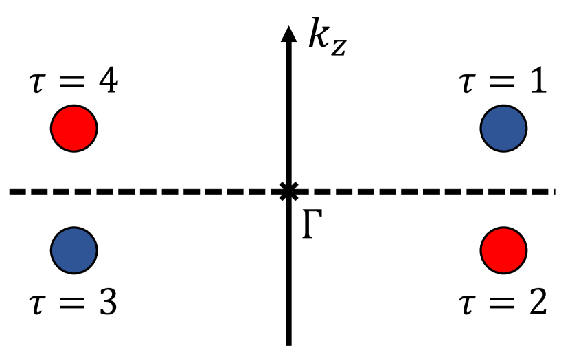
Figure 1: Toy model of a WSM with time-reversal symmetry and a mirror plane perpendicular to the $\widehat{\mathbf{z}}$ direction. The $y$ axis passes through the cross. Blue and red circles indicate Weyl nodes with opposite chiralities.

The low-energy noninteracting single-particle Hamiltonian for an electron in node $\tau$ is given by

$$h_{\tau}(\mathbf{p})=d_{\tau,0}(\mathbf{p})\sigma_{0}+\mathbf{d}_{\tau}(\mathbf{p})\cdot\mathbf{\sigma,}$$ (1)

where $\mathbf{p}$ is the momentum of the electron measured with respect to the Weyl node, $\mathbf{\sigma}$ is a vector of Pauli matrices in the $1/2-$pseudospin state of the two bands at their crossing points and $\sigma_{0}$ is the $2\times 2$ unit matrix. For node $\tau=1,$ we take

$$d_{1,0}(\mathbf{p}) =v_{F}\mathbf{t\cdot p},$$

$$\mathbf{d}_{1}(\mathbf{p}) =v_{F}\mathbf{p},$$ (2)

where $v_{F}$ is the Fermi velocity and $\mathbf{t}$ is a dimensionless vector describing the magnitude and direction of the tilt of the Weyl cone. We restrict our analysis to a type I WSM, i.e. to $\left|\mathbf{t}\right|<1$. The Hamiltonians of the other three Weyl nodes are obtained by applying mirror and time-reversal operations to $h_{1}(\mathbf{p})$. These amount to making the transformations

$$\tau =1\rightarrow 2:(v_{F},t_{x},t_{y},t_{z})\rightarrow(-v_{F},-t_{x},-t_{y},t_{z}),$$

$$\tau =1\rightarrow 3:(v_{F},t_{x},t_{y},t_{z})\rightarrow(v_{F},-t_{x},-t_{y},-t_{z}),$$ (3)

$$\tau =1\rightarrow 4:(v_{F},t_{x},t_{y},t_{z})\rightarrow(-v_{F},t_{x},t_{y},-t_{z}),$$

where we have assumed that $\boldsymbol{\sigma}$ transforms as a spin under time-reversal and mirror operations (see Ref. Bertrand2017, for a discussion of this point).

A transverse static magnetic field $\mathbf{B}_{0}$ is added via the Peierls substitution $\mathbf{p}\rightarrow\mathbf{P}=\mathbf{p}+e\mathbf{A.}$ While it is possible to obtain the energy levels of the hamiltonian analyticallyGoerbig2016 , we find it more convenient to use a numerical approach in order to get a fully orthonormal basis for the eigenspinors. Moreover, a numerical approach allows a study of the system for arbitrary orientations of the magnetic field and tilt vector. It also allows the consideration of more complex Hamiltonians with, for example, non linear terms in the energy spectrumBertrand2017 . The numerical diagonalization of $h_{1}(\mathbf{P})$ is carried out in Appendix A. The many-body Hamiltonian in the basis of the Landau levels of $h_{1}(\mathbf{P})$ can be written as

$$\mathcal{H}=\sum_{\tau,X,p_{\|},I}E_{I}\left(\tau,p_{\|}\right)d_{I}^{{\dagger}}\left(\tau,X,p_{\|}\right)d_{I}\left(\tau,X,p_{\|}\right).$$ (4)

In Eq. (4), the eigenstates are defined by the set of quantum numbers $\left(I,X,p_{\|},\tau\right),$ where $X$ is the guiding-center index and $I=\left(n,s\right)$ the Landau level index. Our convention is to take $n=0,1,2,3,...$ as a positive number and use $s=+1\left(-1\right)$ for the positive (negative)-energy levels. The variable $p_{\|}=\hslash k_{\|}$ is the momentum in the direction of the magnetic field, which we set along the $z$ (or $x$) axis, i.e. perpendicular (or parallel) to the mirror plane. Each Landau level $\left(I,p_{\|},\tau\right)$ has the macroscopic degeneracy $N_{\varphi}=S/2\pi\ell^{2},$ where $\ell=\sqrt{\hslash/eB_{0}}$ is the magnetic length and $S$ is the area of the WSM perpendicular to the magnetic field. The operator $d_{I}^{{\dagger}}\left(\tau,X,p_{\|}\right)$ creates an electron in the quantum state $\left(I,p_{\|},X,\tau\right).$

The dispersion of the Landau levels is given in Figs. 2 and 3 for $\mathbf{t}\perp\mathbf{B}$ and $\mathbf{t}||\mathbf{B}$, respectively. The arrows in these figures indicate the energy gap for interband transitions when the Fermi level $E_{F}$ is in the chiral Landau level (i.e. $n=0$). The optical gaps are identical for all nodes when the tilt and magnetic field are perpendicular to each other. When the magnetic field is perpendicular to the mirror plane and has a nonzero projection along the tilt vector, the optical gaps for interband transitions involving the chiral Landau level are different for nodes that are related by time-reversal symmetry when $\textbf{B}_{0}=0$, but equal for nodes that are mirror partners (see Ref. Bertrand2019, for a discussion on general orientations of B). When light propagates along the direction of the magnetic field, this difference in the absorption gap leads to a full valley polarizationBertrand2019 .

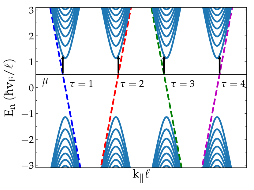
Figure 2: Dispersion of the first Landau levels of the four nodes for $\mathbf{t}=t\widehat{\mathbf{z}}$ and $\mathbf{B}=B_{0}\widehat{\mathbf{x}}.$ The length of each arrow indicates the lowest-energy interband transition under right circularly polarized light. When the tilt vectors of the nodes are perpendicular to the static magnetic field, all nodes have the same interband absorption threshold. For clarity, the position of the different nodes has been shifted in $k_{\|}\ell.$

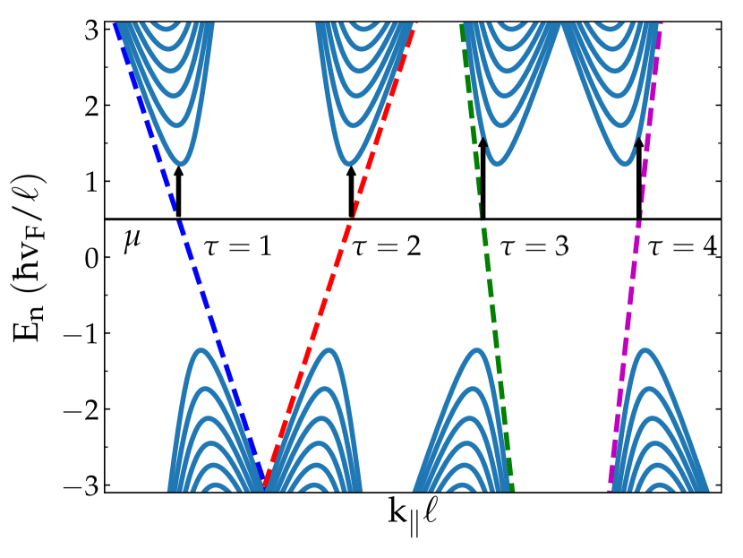
Figure 3: Dispersion of the Landau levels for the four nodes for $\mathbf{t}=t\widehat{\mathbf{z}}$ and $\mathbf{B}=B_{0}\widehat{\mathbf{z}}$. The length of each arrow indicates the lowest-energy interband transition under right circularly polarized light. When the tilt vectors of the nodes have nonzero components along the static magnetic field, different pairs of nodes have different interband absorption thresholds in the quantum limit, thereby leading to a valley polarization. For clarity, the position of the different nodes has been shifted in $k_{\|}\ell.$

III OPTICAL CONDUCTIVITY

The magneto-optical conductivity of Weyl semimetals has been calculated beforeAshby . The effect of a tilt on the ac optical response has also been considered in a model of a WSM with broken TRS and no quantizing magnetic fieldmukherjee . Here we consider the effect of a tilt on the four-node model introduced above (which has TRS) and in the presence of a quantizing magnetic field. We restrict ourselves to $T=0$K. Since we are mainly interested in the behavior of the Kerr angle in the resonant regime, i.e. in the THz range of frequencies, finite temperature effects should be negligible for experiments carried out at low temperature, i.e. at a few Kelvin.

The single-particle current operator for node $\tau$is defined by

$$\mathbf{j}_{\tau}=-\left.\frac{\partial h_{\tau}(\mathbf{p})}{\partial\mathbf{A}_{ext}}\right|_{\mathbf{A}_{ext}\rightarrow 0}=-ev_{F}\left(\mathbf{\sigma}+\mathbf{t}\sigma_{0}\right),$$ (5)

where $\mathbf{A}_{ext}$ is the vector potential of an external electromagnetic field. The many-body current is

$$\mathbf{J}_{\tau} = \int d^{3}r\psi_{\tau}^{{\dagger}}\left(\mathbf{r}\right)\mathbf{j}_{\tau}\psi_{\tau}\left(\mathbf{r}\right)$$

$$= -ev_{F}\sum_{\tau,p_{\|},X}\sum_{I,J}\mathbf{\Upsilon}_{I,J}\left(\tau,p_{\|}\right)d_{I}^{{\dagger}}\left(\tau,X,p_{\|}\right)d_{J}\left(\tau,X,p_{\|}\right),$$

where the matrix elements $\mathbf{\Upsilon}_{I,J}\left(\tau,p_{\|}\right)$ are given in Eq. (87) of Appendix B.

It is convenient to define the operator

$$\rho_{I,J}\left(\tau,p_{\|}\right)=\frac{1}{N_{\varphi}}\sum_{X}d_{I}^{{\dagger}}\left(\tau,X,p_{\|}\right)d_{J}\left(\tau,X,p_{\|}\right),$$ (7)

so that the many-body Hamiltonian and current can be written as

$$\mathcal{H}=\sum_{\tau,p_{\|},I}E_{I}\left(\tau,p_{\|}\right)\rho_{I,I}\left(\tau,p_{\|}\right)$$ (8)

and

$$\mathbf{J}_{\tau}=-ev_{F}\sum_{p_{\|}}\sum_{I,J}\mathbf{\Upsilon}_{I,J}\left(\tau,p_{\|}\right)\rho_{I,J}\left(\tau,p_{\|}\right).$$ (9)

The optical conductivity tensor is related to the retarded current response function $\chi_{\alpha,\beta}^{R}(\omega)=\chi_{\alpha\beta}^{R}(\mathbf{q}=0,\omega)$ by

$$\sigma_{\alpha,\beta}(\omega)=\frac{i}{\omega}\left[\chi_{\alpha,\beta}^{R}(\omega)-\chi_{\alpha,\beta}^{R}(0)\delta_{\alpha\beta}\right],$$ (10)

where $\alpha,\beta\in\left\{x,y,z\right\}$ and $\omega$ is the frequency of the incoming light beam. The diamagnetic contribution to the current operator is lacking in the continuum approximation of the linear spectrum of the low-energy model. This absence leads to unphysical termsKerr Randeria in $\sigma_{\alpha,\beta}(\omega)$. The second term on the right hand side of Eq. (10) is required in order to remove these spurious contributions.

The retarded current response function can be obtained from the two-particle Matsubara Green’s function

$$\chi_{\alpha,\beta}\left(\tau\right) = -\frac{1}{\hslash V}\left\langle T_{\tau}J_{\alpha}\left(\tau\right)J_{\beta}\left(0\right)\right\rangle$$

$$= -e^{2}v_{F}^{2}\frac{1}{\hslash V}\sum_{I,J}\sum_{K,L}\sum_{p_{\|},p_{\|}^{\prime}}\Upsilon_{I,J}^{\left(\alpha\right)}\left(p_{\|}\right)\Upsilon_{K,L}^{\left(\beta\right)}\left(p_{\|}^{\prime}\right)$$

$$\times\left\langle T_{\tau}\rho_{I,J}\left(\tau,p_{\|}\right)\rho_{K,L}\left(0,p_{\|}^{\prime}\right)\right\rangle,$$

where $T_{\tau}$ is the time ordering operator and $\tau$ an imaginary time, not to be confused with the node index. We omit the node index in the remaining of this section in order to avoid any confusion. In linear response, $\chi_{\alpha,\beta}\left(\tau\right)$ is approximated by

$$\chi_{\alpha,\beta}\left(\tau\right) = e^{2}v_{F}^{2}\frac{1}{\hslash V}\sum_{I,J}\sum_{X,p_{\|}}\Upsilon_{I,J}^{\left(\alpha\right)}\left(p_{\|}\right)\Upsilon_{J,I}^{\left(\beta\right)}\left(p_{\|}\right)$$

$$\times G_{I,X}\left(p_{\|},-\tau\right)G_{J,X}\left(p_{\|},\tau\right),$$

where the single-particle Matsubara Green’s function is defined by

$$G_{I,X}\left(p_{\|},\tau\right)=-\left\langle T_{\tau}d_{I}\left(p_{\|},\tau\right)d_{I}^{{\dagger}}\left(p_{\|},0\right)\right\rangle.$$ (13)

Fourier-transforming $\chi_{\alpha,\beta}\left(\tau\right),$ we get the familiar result

$$\chi_{\alpha,\beta}\left(i\Omega_{p}\right) = \int_{0}^{\beta\hslash}d\tau e^{i\Omega_{p}\tau}\chi_{\alpha,\beta}\left(\tau\right)$$

$$= \frac{e^{2}v_{F}^{2}}{\beta\hslash^{2}V}\sum_{\omega_{n}}\sum_{I,J}\sum_{X,p_{\|}}\Upsilon_{I,J}^{\left(\alpha\right)}\left(p_{\|}\right)\Upsilon_{J,I}^{\left(\beta\right)}\left(p_{\|}\right)$$

$$\times G_{I,X}\left(p_{\|},i\omega_{n}\right)G_{J,X}\left(p_{\|},i\Omega_{p}+i\omega_{n}\right),$$

where $\Omega_{p},\omega_{n}$ are respectively bosonic and fermionic Matsubara frequencies. The current-current response has contributions from both intra- and inter-Landau level transitions. We compute them separately in the following sections. Moreover, the total current response and the related dielectric tensor are obtained by summing the individual current response of the four nodes.

III.1 Inter-Landau-level contributions to the current response function $\chi_{\alpha,\beta}\left(\omega\right)$

With the Hamiltonian given by Eq. (4), the single-particle Matsubara Green’s function is simply

$$G_{I,X}\left(p_{\|},i\omega_{n}\right)=\frac{1}{i\omega_{n}-\left(E_{I}\left(p_{\|}\right)-\mu\right)/\hslash},$$ (15)

where $\mu$ is the chemical potential. It is independent of the guiding-center index $X.$

Performing the frequency sum in Eq. (III) and taking the analytic continuation $i\Omega_{p}\rightarrow\omega+i\delta,$ we get for each node $\tau$ the interband response function

$$\chi_{\alpha,\beta}^{R}\left(\omega\right) = -\frac{e^{2}v_{F}^{2}}{4\pi^{2}\ell^{2}\hslash^{2}}\sum_{\begin{subarray}{c}I,J\\ \left(I\neq J\right)\end{subarray}}\int dp_{\|}\Upsilon_{I,J}^{\left(\alpha\right)}\left(p_{\|}\right)\Upsilon_{J,I}^{\left(\beta\right)}\left(p_{\|}\right)$$ (16)

$$\times\frac{f\left(E_{J}\left(p_{\|}\right)\right)-f\left(E_{I}\left(p_{\|}\right)\right)}{\omega+i\delta-\left(E_{J}\left(p_{\|}\right)-E_{I}\left(p_{\|}\right)\right)/\hslash},$$

where $f\left(E\right)=1/(e^{\beta\left(E-\mu\right)}+1)$ is the Fermi function, $\beta=1/k_{B}T$ and $k_{B}$ is the Boltzmann constant. At $T=0$ K, $\mu\rightarrow E_{F}$ and $f\left(E_{J}\left(p_{\|}\right)\right)\rightarrow\Theta\left(E_{F}-E_{J}\left(p_{\|}\right)\right),$ where $\Theta\left(x\right)$ is the step function and $E_{F}$ the Fermi level. Since disorder is not included in our analysis, each Landau level is either filled or empty. It follows that only transitions between an occupied and an unoccupied level can contribute to the response function.

III.2 Intra-Landau-level contribution to the response function $\chi_{\alpha,\beta}\left(\omega\right)$

We consider the situation where the Fermi level lies in the chiral level $n=0,$ above $E=0$ but below the energy of the level $n=1$. The only allowed intra-Landau level transitions are then those that take place in the chiral level. To calculate their contribution to the current response function, disorder needs to be considered. The spectral representation of the disorder-averaged single-particle Green’s function in level $n=0$ is given by

$$\left\langle G_{0,X}\left(p_{\|},i\omega_{n}\right)\right\rangle=\int_{-\infty}^{+\infty}d\omega\frac{A_{0}\left(p_{\|},\omega\right)}{i\omega_{n}-\omega},$$ (17)

with the spectral weight approximated by the Lorentzian shape

$$A_{0}\left(p_{\|},\omega\right)=\frac{\Gamma/\pi}{\left(\omega-\left(E_{0}\left(p_{\|}\right)-\mu\right)/\hslash\right)^{2}+\Gamma^{2}},$$ (18)

where $\Gamma=1/2\tau_{0},$ with $\tau_{0}$ the momentum relaxation time. The current response function becomes

$$\chi_{\alpha,\beta}\left(i\Omega_{p}\right) = \frac{e^{2}v_{F}^{2}N_{\varphi}}{\hslash V}\sum_{p_{\|}}\Upsilon_{0,0}^{\left(\alpha\right)}\left(p_{\|}\right)\Upsilon_{0,0}^{\left(\beta\right)}\left(p_{\|}\right)$$

$$\times\frac{1}{\beta\hslash}\sum_{\omega_{n}}\int_{-\infty}^{+\infty}d\omega^{\prime}\frac{A_{0}\left(p_{\parallel},\omega^{\prime}\right)}{i\Omega_{p}+i\omega_{n}-\omega^{\prime}}$$

$$\times\int_{-\infty}^{+\infty}d\omega^{\prime\prime}\frac{A_{0}\left(p_{\parallel},\omega^{\prime\prime}\right)}{i\omega_{n}-\omega^{\prime\prime}}.$$

Performing the Matsubara frequency sum and taking the analytical continuation $i\Omega_{p}\rightarrow\omega+i\delta$, we get

$$\chi_{\alpha,\beta}^{R}\left(\omega\right) = \frac{e^{2}v_{F}^{2}}{2\pi\ell^{2}\hslash^{2}}\int\frac{dp_{\|}}{2\pi}\Upsilon_{0,0}^{\left(\alpha\right)}\left(p_{\|}\right)\Upsilon_{0,0}^{\left(\beta\right)}\left(p_{\|}\right)$$

$$\times\int_{-\infty}^{+\infty}d\omega^{\prime}\int_{-\infty}^{+\infty}d\omega^{\prime\prime}a_{0}\left(p_{\|},\omega^{\prime}\right)$$

$$\times a_{0}\left(p_{\parallel},\omega^{\prime\prime}\right)\frac{f\left(\omega^{\prime\prime}\right)-f\left(\omega^{\prime}\right)}{\omega+i\delta+\omega^{\prime\prime}-\omega^{\prime}},$$

where we have defined

$$a_{0}\left(p_{\|},\omega\right)=A_{0}\left(p_{\|},\omega+\mu/\hslash\right).$$ (21)

Defining also

$$g_{0}\left(p_{\|},\omega\right)=\frac{\omega-E_{0}\left(p_{\|}\right)/\hslash}{\left(\omega-E_{0}\left(p_{\|}\right)/\hslash\right)^{2}+\Gamma^{2}},$$ (22)

we get, at zero temperature and after some simple algebra

$$\chi_{\alpha\beta}^{R}\left(\omega\right) = \frac{e^{2}v_{F}^{2}}{2\pi\ell^{2}\hslash^{2}}\int\frac{dp_{\|}}{2\pi}\Upsilon_{0,0}^{\left(\alpha\right)}\left(p_{\|}\right)\Upsilon_{0,0}^{\left(\beta\right)}\left(p_{\|}\right)$$

$$\times\left[\int_{-\infty}^{+E_{F}/\hslash}d\omega^{\prime}a_{0}\left(p_{\|},\omega^{\prime}\right)\right.$$

$$\times\left[g_{0}\left(p_{\|},\omega^{\prime}+\omega\right)+g_{0}\left(p_{\|},\omega^{\prime}-\omega\right)\right]$$

$$\left.-i\pi\int_{E_{F}/\hslash-\omega}^{E_{F}/\hslash}d\omega^{\prime}a_{0}\left(p_{\|},\omega^{\prime}\right)a_{0}\left(p_{\|},\omega^{\prime}+\omega\right)\right].$$

Thus, the intraband conductivity in the chiral level is given by

$$\sigma_{\alpha,\beta}^{intra}\left(\omega\right) = \frac{e^{2}v_{F}^{2}}{2\pi\ell^{2}\hslash^{2}}\frac{i}{\omega}\int\frac{dp_{\|}}{2\pi}\Upsilon_{0,0}^{\left(\alpha\right)}\left(p_{\|}\right)\Upsilon_{0,0}^{\left(\beta\right)}\left(p_{\|}\right)$$

$$\times\left[\int_{-\infty}^{+E_{F}/\hslash}d\omega^{\prime}a_{0}\left(p_{\|},\omega^{\prime}\right)K\left(p_{\|},\omega,\omega^{\prime}\right)\right.$$

$$\left.-i\pi\int_{E_{F}/\hslash-\omega}^{E_{F}/\hslash}d\omega^{\prime}a_{0}\left(p_{\|},\omega^{\prime}\right)a_{0}\left(p_{\|},\omega^{\prime}+\omega\right)\right].$$

with the function

$$K\left(p_{\|},\omega,\omega^{\prime}\right) = g_{0}\left(p_{\|},\omega^{\prime}+\omega\right)+g_{0}\left(p_{\|},\omega^{\prime}-\omega\right)$$

$$-2\delta_{\alpha,\beta}g_{0}\left(p_{\|},\omega^{\prime}\right).$$

In the absence of a tilt, only the matrix element $\Upsilon_{0,0}^{\left(\alpha\right)}\left(p_{\|}\right)$ for $\alpha$ in the direction of the magnetic field is nonzero. Thus, only the conductivity $\sigma_{\|}\left(\omega\right)$ (which is $\sigma_{xx}\left(\omega\right)$ for $\mathbf{B}=B_{0}\widehat{\mathbf{x}}$ and $\sigma_{zz}\left(\omega\right)$ for $\mathbf{B}=B_{0}\widehat{\mathbf{z}}$) is nonzero. From Eq. (III.2), we get

$$\operatorname{Re}\left[\sigma_{\|}\left(\omega\right)\right] = \frac{v_{F}e^{3}\tau_{0}}{4\pi^{2}\hslash^{2}}\frac{B_{0}}{1+\left(\omega\tau_{0}\right)^{2}},$$ (26)

$$\operatorname{Im}\left[\sigma_{\|}\left(\omega\right)\right] = \omega\tau_{0}\operatorname{Re}\left[\sigma_{\|}\left(\omega\right)\right].$$ (27)

Our results for the conductivity contains the momentum instead of the transport relaxation time since vertex corrections are not included in our calculation of the current response function.

A finite tilt modifies the matrix elements $\Upsilon_{0,0}^{\left(\alpha\right)}\left(p_{\|}\right)$ and makes the other elements of the conductivity tensor nonzero, in particular $\sigma_{\bot}\left(\omega\right)$ (i.e. $\sigma_{zz}\left(\omega\right)$ for $\mathbf{B}=B_{0}\widehat{\mathbf{x}}$ and $\sigma_{xx}\left(\omega\right)$ for $\mathbf{B}=B_{0}\widehat{\mathbf{z}}$), which enters in the definition of the Kerr angle for the Voigt configuration, as we show below.

With $\tau_{0}$ and $v_{F}$ independent of the magnetic field, Eq. (26) shows that the conductivity $\operatorname{Re}\left[\sigma_{\|}\left(\omega\right)\right]$ increases linearly with the magnetic field. This negative magnetoresistance is a signature of the chiral anomaly in Weyl semimetalsChiral anomaly , where collinear electric and magnetic fields ($\mathbf{E}\cdot\mathbf{B}\neq 0$) result in a transport of electrons between two Weyl nodes of opposite chirality. It is known, however, that $\tau_{0}$ varies with magnetic field in a way that depends on the type of disorder considered. For instance, in the case of short-ranged neutral impurities, $\operatorname{Re}\left[\sigma_{\|}\left(\omega\right)\right]$ becomes independent of $B.$ The $B$-dependence of $v_{F}$ can further alter the sign of the magnetoresistanceDasSarma1 ; Lou2015 . As a result, the $B$-dependence of $\operatorname{Re}\left[\sigma_{\|}\left(\omega\right)\right]$ is not robustly linked to the chiral anomaly.

In contrast, the situation appears to be more promising when it comes to the plasmon frequency $\omega_{p}$. At $q=0$, $\omega_{p}$ is given by the condition

$$\operatorname{Re}\left[\varepsilon_{||}\left(\omega_{p}\right)\right]=0,$$ (28)

i.e.

$$1-\frac{\operatorname{Im}\left[\sigma_{\|}\left(\omega_{p}\right)\right]}{\varepsilon_{0}\omega_{p}}=0,$$ (29)

which gives

$$1-\frac{1}{\varepsilon_{0}}\frac{v_{F}e^{3}}{4\pi^{2}\hslash^{2}}\frac{\tau_{0}^{2}}{1+\left(\omega_{p}\tau_{0}\right)^{2}}B_{0}=0.$$ (30)

The plasmon frequency occurs at high frequency (in the THz range in WSMs), which can exceed the momentum scattering rate. When $\omega_{p}\tau_{0}\gg 1$, one has

$$\omega_{p}^{2}=\frac{e^{2}v_{F}}{4\pi^{2}\hslash\ell^{2}\varepsilon_{0}},$$ (31)

where $\varepsilon_{0}$ is the permittivity of free space (in general to be multiplied by $\varepsilon_{\infty}$ due to screening from high-energy electronic bands). The linear increase with magnetic field of $\omega_{p}^{2}$ is also a signature of the chiral anomalyChiral anomaly and should not be modified by disorder insofar as $\omega_{p}\tau_{0}\gg 1$. This trend remains likewise robust to the $B-$dependence of $v_{F}$ (neglected herein). In a normal metal, the plasmon frequency $\omega_{p,metal}^{2}=n_{e}e^{2}/m\varepsilon_{0},$ with $n_{e}$ the electronic density and $m$ the effective mass of the electron, is independent of the magnetic field (see Appendix C). The dispersion relation of the plasmon mode in WSMs and normal metals are discussed in more detail in Ref. plasmon2, . The plasmon frequency, or equivalently the zero of the longitudinal dielectric function, increases as $\sqrt{B_{0}}$. When interband transitions are considered, $\omega_{p}$ is shifted to a lower frequency as shown in Fig. 4, although it remains in the THz range.

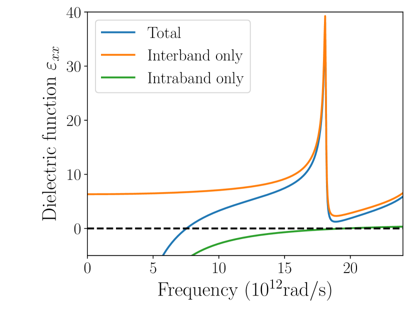
Figure 4: Real part of the relative dielectric function $\varepsilon_{\|}=\varepsilon_{xx}$ as a function of $\omega$ for an external static magnetic field $\mathbf{B}=B_{0}\widehat{\mathbf{x}}$ with $B_{0}=0.3$T. The zero of $\varepsilon_{\|}\left(\omega\right)$, which gives the plasmon frequency, is pushed to a lower frequency when inter-Landau level contributions are considered. Parameters: total electronic density $n_{e}=1\times 10^{20}$ m^-3, momentum relaxation time $\tau_{0}=10$ ps, Fermi velocity $v_{F}=3\times 10^{5}$ m/s, and tilt $t=0.$

IV FORMALISM FOR THE MAGNETO-OPTICAL KERR EFFECT

We consider an electromagnetic wave arriving at normal incidence on a surface of a semi-infinite WSM that has no Fermi arcs. The Maxwell equations in region 1 (the vacuum) and 2 (the WSM) are

$$\mathbf{\nabla\cdot D} = \rho_{f};\ \mathbf{\nabla\times E}=-\frac{\partial\mathbf{B}}{\partial t},$$ (32)

$$\ \mathbf{\nabla\cdot B} = 0;\mathbf{\nabla\times H}=\mathbf{j}_{f}+\frac{\partial\mathbf{D}}{\partial t}\mathbf{,}$$ (33)

where $\rho_{f}$ and $\mathbf{j}_{f}$ are the free charge and current densities. We assume that the WSM is non-magnetic so that $\mathbf{B}=\mu_{0}\mathbf{H}$ with $\mu_{0}$ the permeability of free space. We use the constitutive relation $\mathbf{D}=\epsilon_{0}\overleftrightarrow{\mathbf{\varepsilon}}\cdot\mathbf{E,}$ where $\overleftrightarrow{\mathbf{\varepsilon}}$ is the relative dielectric tensor which is related to the conductivity tensor $\overleftrightarrow{\mathbf{\sigma}}$ by

$$\overleftrightarrow{\mathbf{\varepsilon}}=\overleftrightarrow{\mathbf{I}}+i\frac{\overleftrightarrow{\mathbf{\sigma}}}{\varepsilon_{0}\omega},$$ (34)

with $\overleftrightarrow{\mathbf{I}}$ the unit tensor and $\varepsilon_{0}$ the permittivity of free space. To account for the high-energy transitions not included in our calculation, the unit tensor $\overleftrightarrow{\mathbf{I}}$ should be replaced by the relative dielectric tensor $\overleftrightarrow{\mathbf{\varepsilon}}_{\infty}$ whose precise form depends on the particular WSM considered. In our calculation, we take $\overleftrightarrow{\mathbf{\varepsilon}}_{\infty}=\varepsilon_{\infty}\overleftrightarrow{\mathbf{I}}$ with $\varepsilon_{\infty}=1.$ Because $\varepsilon_{\infty}$ can be quite big in WSMs, we discuss the effects of increasing $\varepsilon_{\infty}$ on the Kerr angle in Sec. VI.

From the Maxwell equations, the dispersion relation of an electromagnetic wave in both regions (with $\overleftrightarrow{\mathbf{\varepsilon}}=\overleftrightarrow{\mathbf{I}}$ in region 1) is given by

$$q^{2}\mathbf{E-}\left(\mathbf{q\cdot E}\right)\mathbf{q=}\frac{\omega^{2}}{c^{2}}\overleftrightarrow{\mathbf{\varepsilon}}\cdot\mathbf{E}.$$ (35)

At the interface between vacuum and WSM, the electromagnetic field must obey the boundary conditions

$$\left(\mathbf{D}_{1}\mathbf{-D}_{2}\right)\cdot\mathbf{\hat{n}} = \sigma_{f},$$ (36)

$$\left(\mathbf{B}_{1}\mathbf{-B}_{2}\right)\cdot\mathbf{\hat{n}} = 0,$$

$$\mathbf{E}_{1}^{\parallel}\mathbf{-E}_{2}^{\parallel} = \mathbf{0},$$

$$\mathbf{H}_{1}^{\parallel}\mathbf{-H}_{2}^{\parallel} = \mathbf{0},$$

where $\mathbf{\hat{n}}$ is a vector normal to the WSM surface, pointing from region 2 to 1. $\mathbf{E}_{i}^{\parallel},\mathbf{H}_{i}^{\parallel}$ (with $i=1,2$) are the field components parallel to the surface of the WSM, which we take to be the $x-y$ plane at $z=0$.

The incident wave is assumed to be linearly polarized in the $x-y$ plane : $\mathbf{E}_{I}(z,t)=(E_{0}^{x}\mathbf{\hat{x}}+E_{0}^{y}\mathbf{\hat{y}})e^{i(qz-\omega t)}.$ Its dispersion relation is $q^{2}=\omega^{2}/c^{2}$, where $c$ is the speed of light in vacuum. The reflected wave is given by

$$\mathbf{E}_{R}(z,t)= [(r_{xx}E_{0}^{x}+r_{xy}E_{0}^{y})\mathbf{\hat{x}}$$ (37)

$$+(r_{yx}E_{0}^{x}+r_{yy}E_{0}^{y})\mathbf{\hat{y}}]e^{-i(qz+\omega t)},$$

where $r_{ij}$ are complex reflection coefficients that depend on the orientation of the magnetic field, tilt vector and mirror plane. We consider two different cases in the following sections: the longitudinal and transverse configurations.

IV.1 Longitudinal propagation $\left(\mathbf{q\parallel B_{0}\parallel\hat{z}}\right)$

In the longitudinal configuration, the electromagnetic wave propagates in the direction of the external magnetic field. If the external magnetic field $\mathbf{B_{0}}$ and the tilt vector $\mathbf{t}$ are in the $\mathbf{\hat{z}}$ direction, perpendicular to the mirror plane, then the total dielectric tensor (sum of the four nodes) has the form

$$\overleftrightarrow{\mathbf{\varepsilon}}=\left(\begin{array}[]{ccc}\varepsilon_{xx}&\varepsilon_{xy}&0\\ -\varepsilon_{xy}&\varepsilon_{xx}&0\\ 0&0&\varepsilon_{zz}\end{array}\right).$$ (38)

In this situation, Maxwell equations support in the WSM two elliptically polarized electromagnetic waves, the analog of the right (RCP) and left (LCP) circularly polarized waves, with electric fields $E_{+}=E_{x}+iE_{y}$ and $E_{-}=E_{x}-iE_{y}$. The transmitted electric fields for these two solutions are given by :

$$\mathbf{E}_{T}^{\left(\pm\right)}(z,t)= [(t_{xx}^{\left(\pm\right)}E_{0}^{x}+t_{xy}^{\left(\pm\right)}E_{0}^{y})\mathbf{\hat{x}}$$ (39)

$$+(t_{yx}^{\left(\pm\right)}E_{0}^{x}+t_{yy}^{\left(\pm\right)}E_{0}^{y})\mathbf{\hat{y}}]e^{-i(q_{\pm}z-\omega t)},$$

where $t_{ij}(\omega)$ are complex transmission coefficients. The component $E_{T,z}=0$ so that the wave is transverse in both media and there is no induced charge (i.e. $\mathbf{\nabla\cdot D}=0$) in the WSM. The dispersion relations are

$$q_{\pm}^{2}(\omega) = \frac{\omega^{2}}{c^{2}}\left(\varepsilon_{xx}\pm i\varepsilon_{xy}\right)$$

$$\equiv \frac{\omega^{2}}{c^{2}}\varepsilon_{\mp}\left(\omega\right)$$

$$= q^{2}\varepsilon_{\mp}\left(\omega\right)$$

with $q=\omega/c.$

The total electric fields in regions 1 and 2 are given by

$$\mathbf{E}_{1}(z,t) = \mathbf{E}_{I}(z,t)+\mathbf{E}_{R}(z,t),$$ (41)

$$\mathbf{E}_{2}(z,t) = \mathbf{E}_{T}^{+}(z,t)+\mathbf{E}_{T}^{-}(z,t),$$ (42)

with the magnetic fields obtained from Faraday’s law.

Applying the boundary conditions to the total electric and magnetic field and isolating the reflection coefficients, we get

$$r_{xx}(\omega) =r_{yy}(\omega)=\frac{1-\sqrt{\varepsilon_{+}\varepsilon_{-}}}{\left(1+\sqrt{\varepsilon_{+}}\right)\left(1+\sqrt{\varepsilon_{-}}\right)},$$ (43a)

$$r_{yx}(\omega) =-r_{xy}(\omega)=\frac{i\left(\sqrt{\varepsilon_{+}}-\sqrt{\varepsilon_{-}}\right)}{\left(1+\sqrt{\varepsilon_{+}}\right)\left(1+\sqrt{\varepsilon_{-}}\right)}.$$ (43b)

In this configuration, the incident wave is taken to be linearly polarized at an angle $\theta_{I}=\pi/4$ from the $x$ axis with amplitude $E_{0}^{x}$ along both directions of the $x-y$ plane, so that the reflected electric field is

$$\mathbf{E}_{R}(z,t)=\left(E_{R}^{x}(\omega)\mathbf{\hat{x}}+E_{R}^{y}(\omega)\widehat{\mathbf{y}}\right)e^{-i(qz+\omega t)},$$ (44)

with

$$E_{R}^{x}(\omega) = \left(r_{xx}(\omega)+r_{xy}(\omega)\right)E_{0}^{x},$$ (45)

$$E_{R}^{y}(\omega) = \left(r_{xx}(\omega)-r_{xy}(\omega)\right)E_{0}^{x}.$$ (46)

The coefficients $r_{ij}(\omega)$ are obtained from the dielectric tensor $\overleftrightarrow{\mathbf{\varepsilon}},$ which contains the combined current response function of the four nodes.

IV.2 Transverse propagation $\left(\mathbf{q\perp\mathbf{B_{0}}\parallel\hat{x}}\right)$

In the transverse configuration, the electromagnetic wave still propagates along the $z$ axis, but the external magnetic field is taken to point in the direction $\mathbf{\hat{x},}$ i.e. parallel to the mirror plane. For a tilt along the $z$ axis, the dielectric tensor for this configuration has the form

$$\overleftrightarrow{\varepsilon}=\left(\begin{array}[]{ccc}\varepsilon_{xx}&0&0\\ 0&\varepsilon_{yy}&\varepsilon_{yz}\\ 0&-\varepsilon_{yz}&\varepsilon_{zz}\end{array}\right)$$ (47)

when the contributions of the four nodes are taken into account.

Maxwell’s equations give again two dispersion relations: one where the electric field $\mathbf{E}_{\|}$ of the incident light is polarized along $x,$ i.e. parallel to the static magnetic field, giving the dispersion relation

$$q_{\parallel}^{2}=\frac{\omega^{2}}{c^{2}}\varepsilon_{xx},$$ (48)

and one where the electromagnetic wave is polarized along $y,$ i.e. perpendicular to the static magnetic field with the dispersion relation

$$q_{\perp}^{2}=\frac{\omega^{2}}{c^{2}}\left(\varepsilon_{yy}+\frac{\varepsilon_{yz}^{2}}{\varepsilon_{zz}}\right)=\frac{\omega^{2}}{c^{2}}\varepsilon_{v},$$ (49)

where $\varepsilon_{v}$ is called the Voigt dielectric functionBalkansky . In this later case, there is an induced field in the direction of propagation, given by

$$E_{z}=-\frac{\varepsilon_{zy}}{\varepsilon_{zz}}E_{y},$$ (50)

so that the electric field for this polarization, in medium 2, is given by

$$\mathbf{E}_{\bot}=E_{y}\left(\widehat{\mathbf{y}}-\frac{\varepsilon_{zy}}{\varepsilon_{zz}}\widehat{\mathbf{z}}\right).$$ (51)

The induced charge is still zero, however. The transmitted wave in the WSM is given by

$$\mathbf{E}_{T}^{\left(\pm\right)}(z,t)=t_{\|}\mathbf{E}_{\|}e^{-i(q_{\|}z-\omega t)}+t_{\bot}\mathbf{E}_{\bot}e^{-i(q_{\bot}z-\omega t)},$$ (52)

where $t_{\|},t_{\bot}$ are the transmission coefficients for the parallel and transverse polarizations. In the Voigt configuration, the polarization vector of an incident electromagnetic wave polarized at an angle with respect to the $x$ axis in the $x-y$ plane will rotate in the WSM because of the different refractive indices for the parallel and transverse polarizations. There is no rotation if the polarization vector is only along the $x$ or $y$ axis. This form of dichroism can also lead to a sizeable Kerr rotation as we show in Sec. V. Solving Eqs. (35) and (36) gives the reflected field components

$$E_{R}^{x}(\omega) = \frac{1-\sqrt{\varepsilon_{xx}}}{1+\sqrt{\varepsilon_{xx}}}E_{0}^{x}(\omega),$$ (53)

$$E_{R}^{y}(\omega) = \frac{1-\sqrt{\varepsilon_{v}}}{1+\sqrt{\varepsilon_{v}}}E_{0}^{y}(\omega).$$

IV.3 Definition of the Kerr angle

We define the phases $\theta_{R}^{x}$ and $\theta_{R}^{y}$ by

$$E_{R}^{x}=\left|E_{R}^{x}\right|^{i\theta_{R}^{x}},\;E_{R}^{y}=\left|E_{R}^{y}\right|e^{i\theta_{R}^{y}},$$ (54)

where $\left|E_{R}^{i}\right|,\theta_{R}^{i}$ (with $i=x,y$) are respectively the moduli and associated phases of the complex components of the reflected wave. The reflected electric field at $z=0$ is then

$$\mathbf{E}\left(t\right)=\left|E_{R}^{x}\right|\cos\left(\theta_{R}^{x}-\omega t\right)\widehat{\mathbf{x}}+\left|E_{R}^{y}\right|\cos\left(\theta_{R}^{y}-\omega t\right)\widehat{\mathbf{y}}.$$ (55)

The polarization of the reflected field is strongly modified as the frequency is varied. It could be linear, elliptical or circular. The sense of rotation of the polarization can also change with $\omega.$ A complete description of the reflected field would give $\mathbf{E}\left(t\right)$ over one period of oscillation. Experimentally, however, what is reported is the Kerr angle $\theta_{K}$ and ellipticity $\phi_{K}$ defined by

$$\tan\left(\theta_{K}+\theta_{I}\right)=\left|\frac{E_{R}^{y}}{E_{R}^{x}}\right|,$$ (56)

where $\theta_{I}$ is the polarization angle of the incident linearly polarized wave, and the ellipticity

$$\phi_{K}=\theta_{R}^{x}-\theta_{R}^{y}.$$ (57)

In the Faraday configuration, with an incident wave linearly polarized at an angle $\theta_{I}=\pi/4$ with respect to the $x$ axis, the Kerr angle is given by

$$\tan\left(\theta_{K}+\theta_{I}\right)=\left|\frac{1+i\left(\sqrt{\varepsilon_{+}}-\sqrt{\varepsilon_{-}}\right)-\sqrt{\varepsilon_{+}\varepsilon_{-}}}{1-i\left(\sqrt{\varepsilon_{+}}-\sqrt{\varepsilon_{-}}\right)-\sqrt{\varepsilon_{+}\varepsilon_{-}}}\right|,$$ (58)

while in the Voigt configuration for the identically polarized incident wave, the Kerr angle is

$$\tan\left(\theta_{K}+\theta_{I}\right)=\left|\frac{\left(1-\sqrt{\varepsilon_{v}}\right)\left(1+\sqrt{\varepsilon_{xx}}\right)}{\left(1+\sqrt{\varepsilon_{v}}\right)\left(1-\sqrt{\varepsilon_{xx}}\right)}\right|.$$ (59)

V NUMERICAL RESULTS FOR THE KERR ANGLE

We compute the Kerr angle in the four-node model for two specific configurations: (1) the longitudinal Faraday configuration where $\mathbf{q\parallel B}_{0}\mathbf{\parallel\hat{z}}$ and the linear polarization vector is $\widehat{\mathbf{e}}\bot\mathbf{B}_{0};$ and (2) the transverse Voigt configuration where $\mathbf{q\parallel\hat{z},}$ $\mathbf{B}_{0}=B_{0}\widehat{\mathbf{x}}\bot\mathbf{q}$ and the linear polarization vector $\widehat{\mathbf{e}}$ is in the $x-y$ plane. For the Faraday configuration, we choose the magnetic field to be perpendicular to the mirror plane while we take it in the mirror plane in the Voigt configuration. Other choices are, of course, possible. We assume a total electronic density of $n_{e}=1\times 10^{20}$ m^-3 for the four nodes. For the interband transitions, we introduce the scattering rate phenomenologically by taking a finite but small value of $\delta$ in the conductivity tensor. For the intraband transitions, disorder is taken into account explicitly by introducing a lorentzian broadening $\Gamma=1/2\tau_{0}$ with $\tau_{0}=10^{-11}$ s. In both configurations, the tilt vector is taken to be $\mathbf{t}=t_{0}\widehat{\mathbf{z}}$ with $t_{0}=0.5$, so that $\mathbf{t}\|\mathbf{B}_{0}$ in the Faraday configuration and $\mathbf{t}\bot\mathbf{B}_{0}$ in the Voigt configuration. This is done in order to isolate the main features of the Kerr angle in both configurations, i.e. valley polarization in the former, and chiral anomaly in the latter. In the presentation of our results, we change the notation for the Landau level index, i.e. we choose $n$ to be positive for $s=+1$ and negative for $s=-1.$ The chiral Landau level is still $n=0.$

V.1 Faraday configuration

When the external magnetic field has a non-zero projection along the tilt vector, an optical valley polarization effect appears in the absorption spectrum. This effect results in a splitting of the interband transition peaks $0\rightarrow\left|n\right|$ and $-\left|n\right|\rightarrow 0$ that involve the chiral Landau level. One pair of nodes starts absorbing light before the other pair, leading to a valley polarization. This phenomenon was studied extensively in our previous work on the absorption spectrum of a WSMBertrand2019 . Here, we show that it is also possible to probe it using the MOKE.

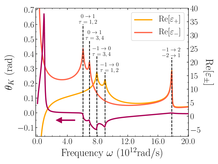
Figure 5: Frequency dependence of the Kerr angle $\theta_{K}$ and real part of the dielectric functions $\varepsilon_{+}$ and $\varepsilon_{-}$ in the Faraday configuration, where $\mathbf{q},\mathbf{B}_{0},\mathbf{t\parallel}\widehat{\mathbf{z}}$. The interband transitions contributing to the main peaks are indicated. The $0\rightarrow 1$ and $-1\rightarrow 0$ transitions are each split into two as a consequence of valley polarization; the Weyl nodes $\tau$ contributing to each of the subpeaks are indicated. Parameters: $B_{0}=0.2$T, $n_{e}=1\times 10^{20}$ m^-3, $v_{F}=3\times 10^{5}$ m/s, $\mathbf{t}=0.5\widehat{\mathbf{z}}.$

A plot of the Kerr angle versus frequency is shown in Fig. 5 for the case where the vectors $\mathbf{q},\mathbf{B}_{0},\mathbf{t}$ are all parallel to the $z$ axis and so perpendicular to the mirror plane. The incident wave is assumed linearly polarized in the $x-y$ plane with $\theta_{I}=\pi/4$ and the Fermi level is in the chiral Landau level. In this configuration, only the dipolar transitions are permitted. The allowed interband transitions are visible as a succession of dips in the curve of the Kerr angle vs frequency for $\omega\gtrsim 4\times 10^{12}$ rad/s or peaks in the dielectric functions $\operatorname{Re}\left[\varepsilon_{\pm}\left(\omega\right)\right]$. The curve of $\theta_{K}\left(\omega\right)$ shows a large peak around $\omega\approx 1\times 10^{12}$ rad/s, which coincides with the frequency $\omega_{+}$ where $\operatorname{Re}\left[\varepsilon_{+}\left(\omega\right)\right]=0$. Figure 6 shows that this large peak in $\theta_{K}\left(\omega\right)$ is redshifted in frequency when the magnetic field increases, which is also the behavior of the frequency $\omega_{+}\left(B\right).$ A similar shift happens in a normal metal (see Appendix C). We remark that $\tau_{0}$ does not enter in the calculation of the Kerr angle, i.e. in Eq. (58), in this configuration.

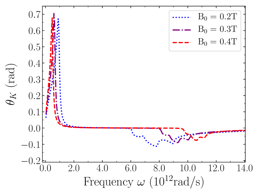
Figure 6: Kerr angle as a function of frequency for different values of the magnetic field $\mathbf{B}=B_{0}\widehat{\mathbf{z}}$ in the Faraday configuration. Parameters: $n_{e}=1\times 10^{20}$ m^-3, $v_{F}=3\times 10^{5}$ m/s, $\mathbf{t}=0.5\widehat{\mathbf{z}}.$

Figure 5 shows that nodes related by time-reversal symmetry (TRS), i.e. nodes 1 and 3 or 2 and 4, have different optical gaps in the Faraday configuration. This causes a splitting of the dips in $\theta_{K}\left(\omega\right)$ or the peaks in $\operatorname{Re}\left[\varepsilon_{\pm}\left(\omega\right)\right]$ corresponding to the transitions $0\rightarrow 1$ and $-1\rightarrow 0$. (Note that we could have chosen a different Faraday configuration leading to no splitting.) The other interband peaks in $\operatorname{Re}\left[\varepsilon_{\pm}\left(\omega\right)\right]$, corresponding to transitions between nonchiral Landau levels, are not split. By contrast, when $\mathbf{t\cdot B}_{0}=0$ for all nodes, transitions $0\rightarrow 1$ (or $-1\rightarrow 0$) are equivalent for all four nodes and therefore, only a single dip or peak is present for each transition $0\rightarrow 1$ or $-1\rightarrow 0$. With a linearly polarized incident wave, both $0\rightarrow 1$ and $-1\rightarrow 0$ transitions are excited. For a circularly polarized light, either the $0\rightarrow 1$ or $-1\rightarrow 0$ transition is excited. (More specifically, the transitions $\left|n\right|\rightarrow\left|n\right|+1$ show up in $\varepsilon_{-}$ and the transitions $\left|n\right|\rightarrow\left|n\right|-1$ in $\varepsilon_{+}$, as in graphene.) The valley polarization effect due to a finite tilt, for transitions involving the chiral level, are thus detectable in the Kerr rotation spectra.

Using Eq. (83), the energy gap between two Landau levels $n,m\neq 0$ of a tilted Weyl cone is independent of the node index and increases with magnetic field. As we just showed, the gap involving the chiral level behaves differently. If the Fermi level is not at the neutrality point, it depends on the node index and the splitting of the $0\rightarrow 1$ (or $-1\rightarrow 0$) peak decreases with increasing magnetic field as can be seen in Fig. 6. This behavior is also present in the absorption spectrum (see Fig. 9 of Ref. Bertrand2019, ). It follows that, in the quantum limit, the valley polarization is present in the Kerr rotation angle in a larger range of frequencies as the magnetic field is decreased. The splitting can also be increased by increasing the tilt. It would be interesting to measure these effects experimentally.

V.2 Voigt configuration

In the Voigt configuration, the magnetic field $\mathbf{B}=B_{0}\widehat{\mathbf{x}}$ is perpendicular to the propagation vector $\mathbf{q\parallel\hat{z}}$ and the tilt vector $\mathbf{t\parallel\hat{z}}$ and the polarization vector $\widehat{\mathbf{e}}$ lies in the $x-y$ plane. As Eq. (53) shows, in order to see a Kerr rotation in the Voigt configuration, the polarization of the incident wave propagating along the $z$ direction must make an angle with the $x$ and $y$ axis. We choose $\theta_{I}=\pi/4$ and $E_{0}^{x}=E_{0}^{y}=E_{0}$ for the incoming electric field. Then, the reflected electric field is given by

$$E_{R}^{x}(\omega) = \frac{1-\sqrt{\varepsilon_{xx}}}{1+\sqrt{\varepsilon_{xx}}}E_{0}(\omega),$$ (60)

$$E_{R}^{y}(\omega) = \frac{1-\sqrt{\varepsilon_{v}}}{1+\sqrt{\varepsilon_{v}}}E_{0}(\omega),$$

with $\varepsilon_{v}=\varepsilon_{yy}+\varepsilon_{yz}^{2}/\varepsilon_{zz}.$

We first remark that if interband transitions are not included in the calculation of the dielectric functions, then $\varepsilon_{yy}=1$ and $\varepsilon_{yz}=0$ so that $\varepsilon_{v}=1.$ It then follows from Eq. (60) that $E_{R}^{y}(\omega)=0$, and so $\tan\left(\theta_{K}+\theta_{I}\right)=0$, giving $\theta_{K}=-\pi/4.$ There is no structure in the Kerr angle in this case. When both intraband and interband transitions are included, the behavior of the Kerr angle with frequency and magnetic field is shown in Fig. 7. We notice that the Kerr angle in this configuration is as big as in the Faraday configuration, in contrast to a normal metal (where it is at least ten times smaller). Moreover, its behavior is clearly different from that in the Faraday configuration. The strong peak in the Kerr angle at high frequency occurs when $\operatorname{Re}\left[\varepsilon_{xx}\left(\omega\right)\right]=0,$ i.e. at the WSM plasmon frequency $\omega=\omega_{p}$ given by Eq. (31), as can be seen in Fig. 8. The peak is also present at zero tilt, and its frequency increases as $\sqrt{B_{0}}$. In an ordinary metal, the frequency of the peak in the Kerr angle increases proportionally to $B_{0}^{2}$. Moreover, in a metal, the negative peak in the Kerr angle occurs at the plasmon frequency $\omega_{p,metal}=\sqrt{ne^{2}/m\varepsilon_{0}}$, which is independent of $B_{0}$. In contrast, in a WSM, the negative peak occurs when $\operatorname{Re}\left[\varepsilon_{v}\left(\omega\right)\right]=0$ (see Fig. 8) and is redshifted with magnetic field. In this figure, the plasmon frequency is below the interband absorption threshold. This is a common circumstance, especially if we take into account the effect of $\epsilon_{\infty}$ which reduces the plasmon frequency without changing the optical gap for interband transitions.

The blueshift of the Kerr angle in a WSM is consistent with the measurement by Levy et al. (see Fig. 2(d) of Ref. [Levy, ]) of the blueshift of the reflectance edge in the Weyl semimetal TaAs. As we pointed out in Sec. III, this magnetoresistance effect is a signature of the chiral anomaly in a WSM and, as Fig. 7 clearly shows, it is reflected in the displacement of the peak in the Kerr angle. This peak is caused mainly by the intraband contribution of the chiral Landau level to the longitudinal conductivity $\sigma_{xx}$ (i.e. $\sigma_{\|}$). Since it occurs at the plasmon frequency given in Eq. (31), which is independent of $\tau_{0}$ in the limit $\omega_{p}\tau_{0}\gg 1,$ it is not affected by the magnetic-field dependence of $\tau_{0}.$ We have checked numerically that taking $\tau_{0}\propto 1/B_{0}$ or $\tau_{0}\propto 1/B_{0}^{2}$ does not change the position of this peak.

The peak disappears if the intraband part of $\sigma_{xx}$ is set to zero, but is almost unchanged if $\sigma_{zz}$ (i.e. $\sigma_{\bot}$) is zero. As discussed in Sec. III, the interband transitions produce a redshift of the plasmon frequency. The shift of the Kerr angle occurs in the THz range and should be measurable in optical experiments. The blueshift of the Kerr angle with magnetic field in the Voigt geometry contrasts with its behavior in the Faraday configuration, where it is redshifted with the magnetic field. The Voigt geometry is special because the longitudinal dielectric function (e.g. $\varepsilon_{xx}$ when $\mathbf{B}_{0}||\hat{\mathbf{x}}$) enters the definition of the Kerr angle, while it does not in the Faraday configuration.

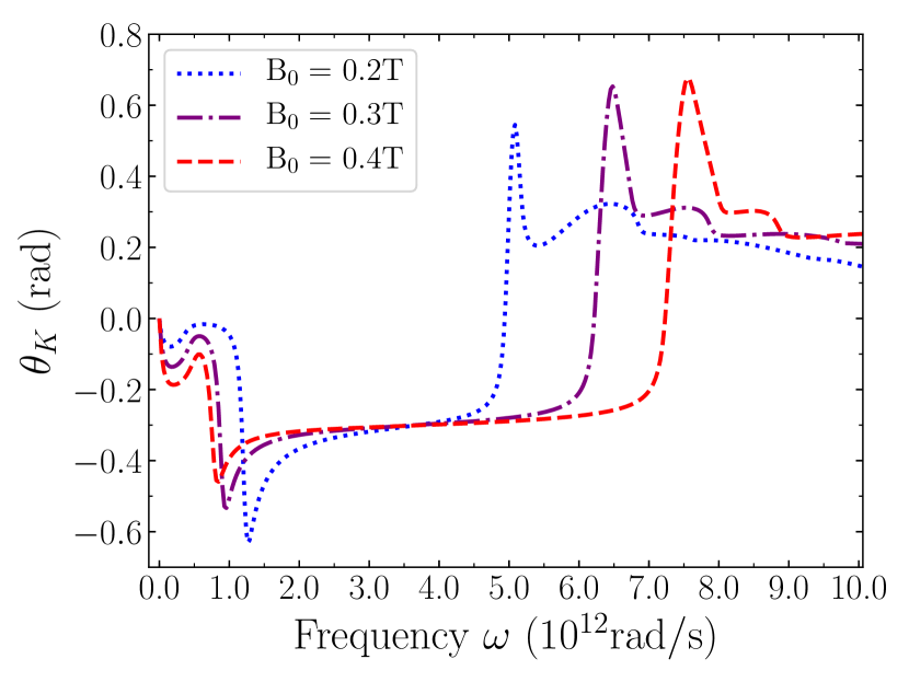
Figure 7: Kerr angle as a function of frequency for different magnetic fields in the Voigt configuration. The blueshift of the large peak in $\theta_{K}$ is related to the chiral anomaly. Parameters: $n_{e}=1\times 10^{20}$ m${}^{-3},\tau_{0}=10$ ps, $v_{F}=3\times 10^{5}$ m/s, $\mathbf{t}=0.5\widehat{\mathbf{z}}.$

Aside from the large maximum caused by intraband transitions, the Kerr angle displays additional smaller peaks originating from interband transitions. The first four of these peaks, also visible in $\operatorname{Re}\left[\varepsilon_{xx}\left(\omega\right)\right]$ (see Fig. 8), occur at the transitions $0\rightarrow 1;$ $-1\rightarrow 0;0\rightarrow 2$ and $-2\rightarrow 0$. Because we choose $\mathbf{t}\bot\mathbf{B}$ (i.e. $t_{\|}=0$ in Eq. (83)), there is no splitting of the $0\rightarrow 1$ and $-1\rightarrow 0$ peaks and so no valley polarization in the Kerr angle.

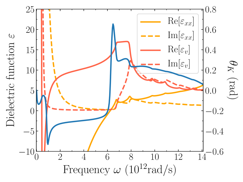
Figure 8: Frequency dependence of the dielectric functions $\varepsilon_{xx}$ and $\varepsilon_{v}$ and of the Kerr angle $\theta_{K}$ for a magnetic field $B=0.3$ T. Parameters: $n_{e}=1\times 10^{20}$ m${}^{-3},\tau_{0}=10$ ps, $v_{F}=3\times 10^{5}$ m/s, $\mathbf{t}=0.5\widehat{\mathbf{z}}.$ The first four peaks in $\operatorname{Re}[\varepsilon_{xx}]$ come from the transitions: $0\rightarrow 1,-1\rightarrow 0,0\rightarrow 2,-2\rightarrow 0.$

Figures 7 and 8 show some intriguing structure in the low-frequency region. However, as this low-frequency behavior will likely be strongly affected by details of the disorder, for example the impact of the $B-$dependence of the scattering time, we will not discuss it further in this paper.

VI SUMMARY

We have shown that a sizeable Kerr rotation is possible in a simplified model of a Weyl semimetal in both the Faraday and Voigt configurations. Inter-Landau level transitions appear as dips or peaks in a plot of the Kerr angle vs frequency and can be detected in this way. Moreover, a tilt of the Weyl cones allows the detection of transitions beyond the dipolar ones. In the particular Faraday configuration that we have chosen to study, with a nonzero tilt of the Weyl cones in the direction of the external magnetic field, the peaks in the Kerr angle that represent interband transitions involving the chiral Landau level are split into subpeaks. This splitting, which we found before in the absorption spectrum, is a manifestation of a full valley polarization in a WSMBertrand2019 . A valley polarization is thus also detectable via the magneto-optical Kerr effect.

We have also demonstrated the interest of measuring the MOKE in the Voigt geometry. In this configuration, the Kerr angle involves the longitudinal dielectric function $\varepsilon_{\|}\left(\omega\right)$, unlike in the Faraday configuration, since the electric field of the wave has a nonzero projection on the external magnetic field. The zero of the longitudinal dielectric function gives the plasmon frequency $\omega_{p}$. The chiral anomaly in a WSM leads to an increase of $\omega_{p}$ with the external static magnetic, i.e. $\omega_{p}\propto\sqrt{B_{0}}$. In the Voigt geometry, a large peak in the Kerr angle $\theta_{K}$ occurs at $\omega_{p}$ and is consequently blueshifted by a magnetic field. We argued that the $\sqrt{B_{0}}$ shift of this peak is the signature of the chiral anomaly in the MOKE, just like the shift of the absorption edge recently reported in reflectance measurementsLevy .

The exact size of the Kerr angle depends, of course, on the dielectric constant $\varepsilon_{\infty}$, which can be quite large in WSMs. We have verified that using a larger value of $\varepsilon_{\infty}$ in our calculation (instead of $\varepsilon_{\infty}=1$) does indeed reduce the amplitude of the Kerr angle signal and redshifts the frequencies of the peaks and dips. For $\varepsilon_{\infty}=30,$ the amplitude of the peak in $\theta_{K}$ at $B=0.3$ T in Fig. 7 is decreased from $0.65$ rad to $0.41$ rad and $\omega_{p}$ is reduced to $\omega_{p}\approx 2.5\times 10^{12}$ rad/s. If $\varepsilon_{\infty}$ is very large, the peak $\theta_{K}\left(\omega_{p}\right)$ may be blurred by disorder. For the chiral anomaly to be detected in the Kerr angle, the plasmon frequency must satisfy the condition $\omega_{p}\tau_{0}\gg 1.$

We have chosen a total electronic density of $n_{e}=1\times 10^{20}$ m^-3 for our calculation, as we did not have a particular WSM in mind. At such a small density, the quantum limit is reached at a very small value of $B_{0}$, i.e. $\approx 0.053$ T. To be certain that this choice does not affect the main conclusions of our paper, and to get a quantum limit closer to recently reported electronic density valuesLevy ; chicheng ; Grassano , we have recalculated Fig. 7 for a much bigger total density of $n_{e}=1\times 10^{22}$ m^-3 and a magnetic field of $B_{0}=7.83$ T (the value of $B_{0}$ needed to obtain the same Fermi level as in Fig. 7 for $B_{0}=0.3$ T). The qualitative aspects of the curve remain unchanged, with almost the same amplitude for the peaks and dips, but with the peak at $\theta_{K}\left(\omega_{p}\right)$ now shifted to $\approx 32\times 10^{12}$ rad/sec, i.e. $\approx 21$ meV. Thus, an increase in the carrier density could compensate for the redshift created by a larger value of $\varepsilon_{\infty}.$

Although our calculations have been carried out for a toy model, the main predictions derived from them are applicable to real WSMs. For example, let us consider TaAs, which displays two symmetry-inequivalent multiplets of Weyl nodes (8 W1 nodes and 16 W2 nodes). If $\mathbf{B}_{0}$ and $\mathbf{q}$ are both parallel to the $c$-axis of the crystal (Faraday configuration), one should see a peak-splitting due to valley polarization in the contribution from the W2 nodes to the Kerr angle. No such splitting would be present in the contribution from the W1 nodes, because these are not tilted along the $c$ axis. In principle, one can distinguish the contributions of the W1 and W2 nodes because their optical absorption thresholds differ by about $10$ meV. Also, if $\mathbf{B}_{0}$ is along the $c$ axis of the crystal but $\mathbf{q}$ is along the $a$ or $b$ axis (Voigt configuration), a peak in the Kerr angle will emulate the blueshift of the plasmon frequency as a function of $B_{0}$. Finally, the contribution from Fermi arcs to the magneto-optical response, neglected in our theory, should not significantly affect our main predictions, as the penetration depth of the electromagnetic waves in weakly doped bulk WSMs can largely exceed the localization length of the surface states.

Appendix A EIGENSTATES OF TILTED WEYL CONES 

A transverse static magnetic field $\mathbf{B}=B_{0}\widehat{\mathbf{z}}$ is added via the Peierls substitution $\mathbf{p}\rightarrow\mathbf{P}=\mathbf{p}+e\mathbf{A,}$ with the vector potential $\mathbf{A}=\left(0,Bx,0\right)$ ($e>0$ for an electron) taken in the Landau gauge. The Hamiltonian $h_{1}(\mathbf{p})$ for node $1$ becomes

$$h_{1}(\mathbf{P})=h_{1}^{\left(0\right)}(\mathbf{P})+W_{1}\left(\mathbf{P}\right),$$ (61)

with

$$h_{1}^{\left(0\right)}(\mathbf{P})=v_{F}\left(\begin{array}[]{cc}P_{z}&P_{x}-iP_{y}\\ P_{x}+iP_{y}&-P_{z}\end{array}\right),$$ (62)

the Hamiltonian in the absence of a tilt, and with

$$W_{1}\left(\mathbf{P}\right)=v_{F}\left(\begin{array}[]{cc}\mathbf{t\cdot P}&0\\ 0&\mathbf{t\cdot P}\end{array}\right),$$ (63)

the perturbation due to the tilt.

The Hamiltonian $h_{1}^{\left(0\right)}(\mathbf{p})$ is easily diagonalized by defining the ladder operators

$$a = \frac{\ell}{\sqrt{2}\hslash}\left(P_{x}-iP_{y}\right),$$ (64)

$$a^{{\dagger}} = \frac{\ell}{\sqrt{2}\hslash}\left(P_{x}+iP_{y}\right).$$ (65)

The energy spectrum of $h_{1}^{\left(0\right)}(\mathbf{p})$ consists in both positive and negative energy Landau levels. We classify them with the indices $n,s$ where $n=0,1,2,3,...$ is always positive and $s=+1\left(-1\right)$ is a band index for the positive(negative) energy levels. For node $1:$

$$E_{1,0}\left(p_{z}\right) = -v_{F}p_{z},$$ (66)

$$E_{1,n\neq 0,s}\left(p_{z}\right) = sv_{F}\sqrt{2\frac{\hslash^{2}}{\ell^{2}}n+p_{z}^{2}},$$ (67)

with the corresponding eigenstates

$$w_{1,n,s,X}\left(p_{z},\mathbf{r}\right)=\frac{1}{\sqrt{L_{z}}}\left(\begin{array}[]{c}u_{1,n,s}\left(p_{z}\right)h_{n-1,X}\left(x,y\right)\\ v_{1,n,s}\left(p_{z}\right)h_{n,X}\left(x,y\right)\end{array}\right)e^{ip_{z}z/\hslash}.$$ (68)

In these equations, $\ell=\sqrt{\hslash/eB}$ is the magnetic length and the wave functions $h_{n,X}\left(x,y\right)$ are the eigenstates of a two-dimensional electron gas in a transverse magnetic field in the Landau gauge:

$$h_{n,X}\left(x,y\right)=\frac{1}{\sqrt{L_{y}}}\varphi_{n}\left(x-X\right)e^{-iXy/\ell^{2}},$$ (69)

with $\varphi_{n}\left(x\right)$ the eigenstates of the one-dimensional harmonic oscillator and $n$ and $X$ the Landau level and guiding-center indices respectively.

The coefficients $u_{1,n,s,p_{z}},v_{1,n,s,p_{z}},$ which are independent of $X,$ are given for $n\neq 0$ by

$$\left(\begin{array}[]{c}u_{1,n,s}\left(p_{z}\right)\\ v_{1,n,s}\left(p_{z}\right)\end{array}\right)=\frac{1}{\sqrt{2}}\left(\begin{array}[]{c}-is\sqrt{1-\frac{v_{F}p_{z}}{E_{1,n,s}\left(p_{z}\right)}}\\ \sqrt{1+\frac{v_{F}p_{z}}{E_{1,n,s}\left(p_{z}\right)}}\end{array}\right),$$ (70)

and obey the normalization condition $\left|u_{1,n,s}\left(p_{z}\right)\right|^{2}+\left|v_{1,n,s}\left(p_{z}\right)\right|^{2}=1.$ For the chiral Landau level $n=0$, the eigenstate is simply

$$\left(\begin{array}[]{c}u_{1,0}\left(p_{z}\right)\\ v_{1,0}\left(p_{z}\right)\end{array}\right)=\left(\begin{array}[]{c}0\\ 1\end{array}\right)$$ (71)

and there is no band index in this case. The eigenenergies are independent of $X$ so that each level $\left(n,s,p_{z}\right)$ has a degeneracy given by $N_{\varphi}=S/2\pi\ell^{2}$ with $S=L_{x}L_{y}$ the area of the electron gas in the $x-y$ plane ($L_{z}$ is its extension in the $z$ direction).

We must now obtain the energies and eigenvectors for tilted cones. Although an analytical solution existsGoerbig2016 , it is more convenient to use a numerical approach to the eigenvalue problem since we can then study the system for arbitrary orientations of the magnetic field and tilt vector or consider more complex Hamiltonians with, for example, non linear terms in the energy spectrumBertrand2017 .

We write the many-body Hamiltonian for the four-node model as

$$\mathcal{H}=\sum_{\tau}\int d^{3}r\psi_{\tau}^{{\dagger}}\left(\mathbf{r}\right)h_{\tau}(\mathbf{r})\psi_{\tau}\left(\mathbf{r}\right)$$ (72)

and expand the fermionic field operators $\psi_{\tau}\left(\mathbf{r}\right)$ onto the $\left\{w_{\tau,n,s,X}\left(p_{z},\mathbf{r}\right)\right\}$ basis (we leave as implicit the fact that $\mathbf{t}$ depends on the node index $\tau$)

$$\psi_{\tau}\left(\mathbf{r}\right)=\sum_{n,X,p_{z}}w_{\tau,n,s,X}\left(p_{z},\mathbf{r}\right)c_{\tau,n,s,X,p_{z}},$$ (73)

where $c_{\tau,n,s,X,p_{z}}$ is the annihilation operator for an electron in the $w_{\tau,n,s,X,p_{z}}\left(\mathbf{r}\right)$ state. The many-body Hamiltonian can be written as

$$\mathcal{H} = \sum_{\tau,n,s,p_{z}}\left(E_{\tau,n,s}\left(p_{z}\right)+v_{F}t_{z}p_{z}\right)c_{\tau,n,s,X,p_{z}}^{{\dagger}}c_{\tau,n,s,X,p_{z}}$$

$$+\frac{\hslash v_{F}}{\sqrt{2}\ell}\sum_{\tau,n,n^{\prime},s,s^{\prime},p_{z}}W_{\tau,n,s,n^{\prime},s^{\prime}}\left(p_{z}\right)c_{\tau,n,s,X,p_{z}}^{{\dagger}}c_{\tau,n^{\prime},s^{\prime},X,p_{z}}.$$

The matrix elements $W_{\tau,n,s,n^{\prime},s^{\prime}}\left(p_{z}\right)$ are defined by

$$W_{\tau,n,s,n^{\prime},s^{\prime}}\left(p_{z}\right) = \int d^{3}rw_{\tau,n,s,X}^{{\dagger}}\left(p_{z},\mathbf{r}\right)$$

$$\times\left(t_{-}a^{{\dagger}}+t_{+}a\right)w_{\tau,n^{\prime},s^{\prime}X}\left(p_{z},\mathbf{r}\right),$$

with the definition

$$t_{\pm}=t_{x}\pm it_{y}.$$ (76)

Their calculation gives

$$W_{\tau,n,s,n^{\prime},s^{\prime}}\left(p_{z}\right)$$

$$= -it_{+}u_{\tau,n,s}^{\ast}\left(p_{z}\right)u_{\tau,n+1,s^{\prime}}\left(p_{z}\right)\sqrt{n}\delta_{n^{\prime},n+1}$$

$$-it_{+}v_{\tau,n,s}^{\ast}\left(p_{z}\right)v_{\tau,n+1,s^{\prime}}\left(p_{z}\right)\sqrt{n+1}\delta_{n^{\prime},n+1}$$

$$+it_{-}u_{\tau,n,s}^{\ast}\left(p_{z}\right)u_{\tau,n-1,s^{\prime}}\left(p_{z}\right)\sqrt{n-1}\delta_{n^{\prime},n-1}$$

$$+it_{-}v_{\tau,n,s}^{\ast}\left(p_{z}\right)v_{\tau,n-1,s^{\prime}}\left(p_{z}\right)\sqrt{n}\delta_{n^{\prime},n-1}.$$

The linear dispersion being valid only in a small region around each Weyl node, an appropriate high-energy cutoff must be applied to the summation over $p_{z}\mathbf{.}$ That cutoff is assumed to be small compared to the internodal separation in momentum space.

We define the super-indices $I=n,s$ and $J=n^{\prime},s^{\prime}$ in order to write the Hamiltonian $\mathcal{H}$ in the matrix form :

$$\mathcal{H}=\sum_{\tau,X,p_{z}}\sum_{I,J}c_{I}^{{\dagger}}\left(\tau,X,p_{z}\right)F_{I,J}\left(\tau,p_{z}\right)c_{J}\left(\tau,X,p_{z}\right),$$ (78)

where $c_{J}\left(\tau,X,p_{z}\right)$ stands for the vector $\left(c_{\tau,1,X,p_{z},}c_{\tau,2,X,p_{z},},c_{\tau,3,X,p_{z},},...,c_{\tau,N,X,p_{z},}\right),$ where $N$ is the number of Landau levels $n,s$ kept in the calculation and $F_{I,J}\left(\tau,p_{z}\right)$ is the $N\times N$ matrix given by

$$F_{I,J}\left(\tau,p_{z}\right)=\left(E_{\tau,I}\left(p_{z}\right)+v_{F}t_{z}p_{z}\right)\delta_{I,J}+W_{\tau,I,J}\left(p_{z}\right),$$ (79)

which is independent of the guiding-center index $X.$

The matrix $\mathbf{F}$ is hermitian and so can be diagonalized by a unitary transformation

$$\mathbf{F}=\mathbf{UDU}^{{\dagger}},$$ (80)

where $\mathbf{U}$ is the matrix of the eigenvectors of $F$ and $D$ the diagonal matrix of its eigenvalues $E_{I}\left(\tau,p_{z}\right),$ which are the energy of the Landau levels in the presence of the tilt.

Defining new operators $d_{I}\left(\tau,X,p_{z}\right)$ by

$$d_{I}\left(\tau,X,p_{z}\right)=\sum_{J}\left(U^{{\dagger}}\right)_{I,J}c_{J}\left(\tau,X,p_{z}\right),$$ (81)

we get the final result

$$\mathcal{H}=\sum_{\tau,X,p_{z}}\sum_{I}E_{I}\left(\tau,p_{z}\right)d_{I}^{{\dagger}}\left(\tau,X,p_{z}\right)d_{I}\left(\tau,X,p_{z}\right).$$ (82)

We also consider the case where the magnetic field is in the $\widehat{\mathbf{x}}$ direction. The analysis proceeds in a similar way.

The analytical resultsGoerbig2016 for the energy levels of the tilted cone $\tau=1$ are

$$E_{n=0,p_{\|}} = v_{F}t_{\|}p_{\|}-\frac{v_{F}}{\gamma}p_{\|},$$ (83)

$$E_{n\neq 0,p_{\|}} = v_{F}t_{\|}p_{\|}+s\frac{1}{\gamma}\sqrt{v_{F}^{2}p_{\|}^{2}+\frac{2\hslash^{2}nv_{F}^{2}}{\gamma\ell^{2}}},$$

where $p_{\|}=\mathbf{p}\cdot\widehat{\mathbf{B}}$, $t_{\|}=\mathbf{t}\cdot\widehat{\mathbf{B}}$ and $\gamma=\left(1-\left|\mathbf{t}\times\widehat{\mathbf{B}}\right|^{2}\right)^{-1/2}.$

Appendix B CURRENT OPERATOR

The single-particle current operator for node $\tau$ is defined by

$$\mathbf{j}_{\tau}=-\left.\frac{\partial h_{\tau}(\mathbf{p})}{\partial\mathbf{A}_{ext}}\right|_{\mathbf{A}_{ext}\rightarrow 0}=-ev_{F}\left(\mathbf{\sigma}+\mathbf{t}\sigma_{0}\right),$$ (84)

where $\mathbf{A}_{ext}$ is the vector potential of an external electromagnetic field. The total many-body current for this node is given by

$$\mathbf{J}_{\tau} = \int d^{3}r\psi_{\tau}^{{\dagger}}\left(\mathbf{r}\right)\mathbf{j}_{\tau}\psi_{\tau}\left(\mathbf{r}\right)$$

$$= -ev_{F}\sum_{\tau,p_{z},X}\sum_{I,J}\mathbf{\Lambda}_{I,J}\left(\tau,p_{z}\right)c_{\tau,I,X,p_{z}}^{{\dagger}}c_{\tau,J,X,p_{z}}$$

$$= -ev_{F}\sum_{\tau,p_{z},X}\sum_{I,J}\mathbf{\Upsilon}_{I,J}\left(\tau,p_{z}\right)d_{I}^{{\dagger}}\left(\tau,X,p_{z}\right)d_{J}\left(\tau,X,p_{z}\right),$$

with the matrix elements defined by

$$\mathbf{\Lambda}_{I,J}\left(\tau,p_{z}\right)=\int d^{3}rw_{\tau,I,X,p_{z}}^{{\dagger}}\left(\mathbf{r}\right)\left(\mathbf{\sigma}+\mathbf{t}\sigma_{0}\right)w_{\tau,J,X,p_{z}}\left(\mathbf{r}\right)$$ (86)

and the definition

$$\mathbf{\Upsilon}=\mathbf{U}^{{\dagger}}\mathbf{\Lambda U.}$$ (87)

The matrix elements

$$\mathbf{\Lambda}_{n,s,n^{\prime},s^{\prime}}$$

$$= u_{\tau,n,s}^{\ast}\left(p_{z}\right)v_{\tau,n-1,s^{\prime}}\left(p_{z}\right)\delta_{n^{\prime},n-1}\left(\widehat{\mathbf{x}}-i\widehat{\mathbf{y}}\right)$$

$$+v_{\tau,n,s}^{\ast}\left(p_{z}\right)u_{\tau,n+1,s^{\prime}}\left(p_{z}\right)\delta_{n^{\prime},n+1}\left(\widehat{\mathbf{x}}+i\widehat{\mathbf{y}}\right)$$

$$+u_{\tau,n,s}^{\ast}\left(p_{z}\right)u_{\tau,n,s^{\prime}}\left(p_{z}\right)\delta_{n^{\prime},n}\widehat{\mathbf{z}}$$

$$-v_{\tau,n,s}^{\ast}\left(p_{z}\right)v_{\tau,n,s^{\prime}}\left(p_{z}\right)\delta_{n^{\prime},n}\widehat{\mathbf{z}}$$

$$+\mathbf{t}\delta_{n,n^{\prime}}\delta_{s,s^{\prime}}.$$

Appendix C MOKE IN A NORMAL METAL

For comparison with the Kerr rotation in a WSM, we give a short review of the Kerr effect in a normal three-dimensional metal in a transverse magnetic field. We consider a system in which the half-space $z<0$ (region 1) is occupied by a non-conducting medium with relative dielectric constant $\varepsilon_{1}=1$ and the half-space $z>0$ (region 2) is occupied by the normal metal. We use the results of Section IV, but with the relative dielectric tensor $\overleftrightarrow{\mathbf{\varepsilon}}$ of a normal metal.

C.1 Longitudinal propagation $\left(\mathbf{q\parallel B}_{\mathbf{0}}\mathbf{\parallel\hat{z}}\right)$

For a magnetic field $\mathbf{B}=B_{0}\mathbf{\hat{z},}$ the (relative) dielectric tensor for a normal metal in the Drude model has the same symmetry as $\overleftrightarrow{\mathbf{\varepsilon}}$ in Eq. (38). The components are given by

$$\varepsilon_{xx} = \varepsilon_{yy}=1-\frac{\omega_{p}^{2}}{\omega}\frac{\omega+\frac{i}{\tau_{m}}}{\left(\omega+\frac{i}{\tau_{m}}\right)^{2}-\omega_{c}^{2}},$$ (89)

$$\varepsilon_{xy} = -\varepsilon_{yx}=\frac{\omega_{p}^{2}}{\omega}\frac{i\omega_{c}}{\left(\omega+\frac{i}{\tau_{m}}\right)^{2}-\omega_{c}^{2}},$$ (90)

$$\varepsilon_{zz} = 1-\frac{\omega_{p}^{2}}{\omega}\frac{1}{\omega+\frac{i}{\tau_{m}}},$$ (91)

where $\tau_{m}$ is the transport relaxation time, $\omega_{c}=eB_{0}/m$ the cyclotron frequency and $\omega_{p}=\sqrt{ne^{2}/\varepsilon_{0}m}$, with $\varepsilon_{0}$ the free space permittivity and $m$ the effective mass of the electrons. The dispersion relation of Eq. (IV.1) for the two circularly polarized electromagnetic waves in a normal metal becomes

$$q_{\pm}(\omega)=\frac{\omega}{c}\sqrt{\varepsilon_{\pm}},$$ (92)

with

$$\varepsilon_{\pm}\left(\omega\right) = \varepsilon_{xx}\mp i\varepsilon_{xy}$$

$$= 1-\frac{\omega_{p}^{2}}{\omega}\left(\frac{1}{\omega\pm\omega_{c}+\frac{i}{\tau_{m}}}\right).$$

In the pure limit ($\tau_{m}\rightarrow\infty$), the zeros of $\varepsilon_{\pm}$ are given by (keeping only positive frequencies)

$$\omega_{\pm}=\frac{\mp\omega_{c}+\sqrt{\omega_{c}^{2}+4\omega_{p}^{2}}}{2}.$$ (94)

We remark that Eq. (C.1) remains valid in the quantum case, when the kinetic energy is quantized into Landau levels.

For an incident wave linearly polarized at $\theta_{I}=\pi/4$ from the $x$ axis with amplitude $E_{0}^{x}$, the reflection coefficients are given by Eqs. (43a)-(43b), the Kerr angle is obtained from Eq. (58) and the phases $\theta_{R}^{x}$ and $\theta_{R}^{y}$ are defined in Eq. (54).

Figure 9 shows the Kerr angle $\theta_{K}$ (left $y$ axis) calculated from Eq. (56) (black line) for the same magnetic fields $B_{0}=0.2,0.3,0.4$ T used in Fig. 7 and the same electronic density (equivalent to the density of one node) $n_{e}=0.25\times 10^{20}$ m${}^{-3}.$ The relaxation time is taken to be $\tau_{m}=10$ ps. As in a WSM, the big peak in the Kerr angle occurs near the zero of the dielectric function $\operatorname{Re}\left[\varepsilon_{+}\left(\omega\right)\right]$ (right $y$ axis), i.e. at $\omega_{+},$ and is shifted to lower frequencies with increasing magnetic field. There is no particular feature of the Kerr angle at the cyclotron frequency $\omega_{c}=eB_{0}/m,$ which is $\omega_{c}=0.035\times 10^{12}$ rad/s for $B=0.2$ T. The density that we use in these calculations is much smaller than that in a normal metal. Our goal is to compare the predictions of the Drude model with that of the WSM, where our numerical calculation uses that particular density.

Figure 10 shows what happens if we increase the density to $n_{e}=0.25\times 10^{22}$ m${}^{-3}.$ There is more structure in the Kerr angle, but the maximum still occurs at $\operatorname{Re}[\varepsilon_{+}\left(\omega_{+}\right)]=0,$ i.e. at a frequency $10$ times bigger, and is again redshifted in frequency by an increasing magnetic field. The shoulder on the left occurs at the smallest of the two zeros of $\operatorname{Re}[\varepsilon_{-}\left(\omega\right)].$ At a density of $n_{e}=1\times 10^{29}$ m${}^{-3},$ typical of a real metal and keeping $\tau_{m}=10$ ps with $B_{0}=10$ T, the Kerr angle is almost constant at $\theta_{K}=0.1$ mrad. It peaks at $\operatorname{Re}[\varepsilon_{+}\left(\omega_{+}\right)]=0,$ i.e. at $\omega_{+}=18.9\times 10^{15}$ rad/s where it reaches $3.5$ mrad. The frequency $\omega_{+}$ is then given by Eq. (94), with $\omega_{c}\tau_{m}\ll\omega_{p}\tau_{m}$ and $\omega_{+}=\omega_{p}.$ The Kerr angle decreases with decreasing value of $\tau_{m}.$

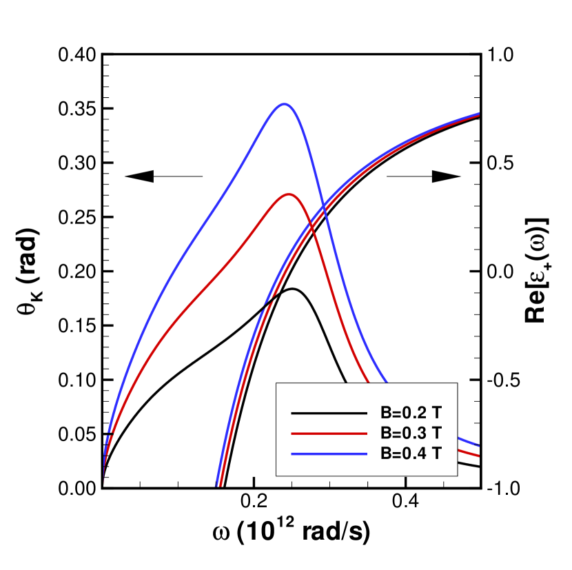
Figure 9: Kerr angle in the Faraday configuration (left $y$ axis) and dielectric function $\operatorname{Re}[\varepsilon_{+}\left(\omega\right)]$ (right $y$ axis) as a function of frequency for an external magnetic field $B_{0}=0.2,0.3,0.4$ and an electronic density $n_{e}=0.25\times 10^{20}$ m^-3.

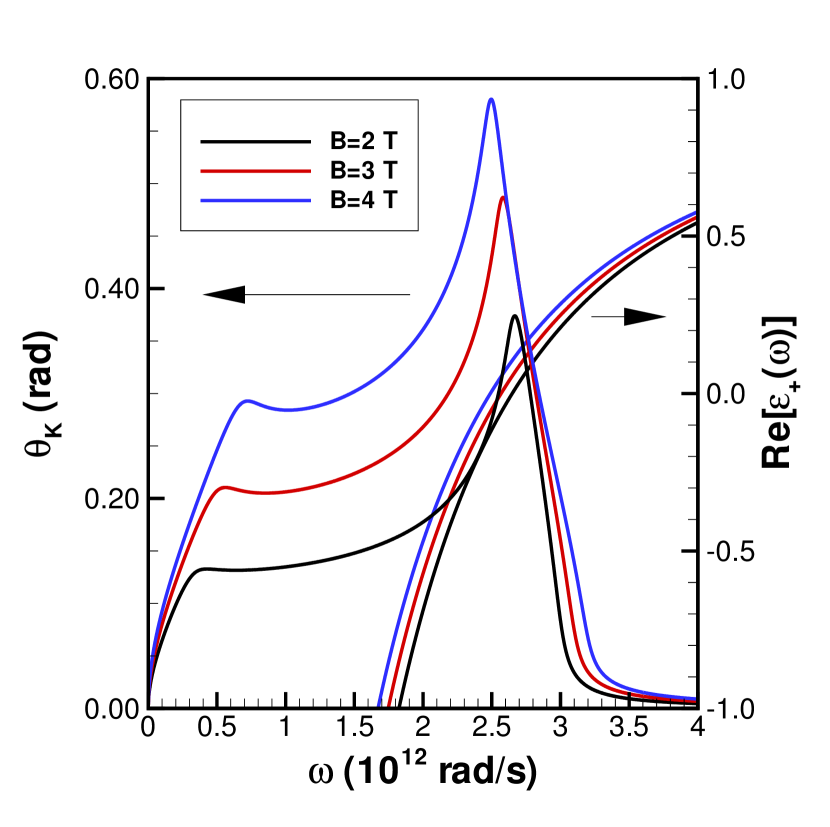
Figure 10: Kerr angle in the Faraday configuration (left $y$ axis) and dielectric function $\operatorname{Re}[\varepsilon_{+}\left(\omega\right)]$ (right $y$ axis) as a function of frequency for an external magnetic field $B_{0}=2,3,4$ and an electronic density $n_{e}=0.25\times 10^{22}$ m^-3

C.2 Transverse propagation $\left(\mathbf{q\perp\mathbf{B}}_{0}\mathbf{\parallel\hat{x}}\right)$

With $\mathbf{B}=B_{0}\widehat{\mathbf{x}},$ the dielectric tensor for a normal metal has the symmetry of $\overleftrightarrow{\mathbf{\varepsilon}}$ in Eq. (47), except that $\varepsilon_{yy}=\varepsilon_{zz}$ and

$$\varepsilon_{xx} = 1-\frac{\omega_{p}^{2}}{\omega}\frac{1}{\left(\omega+\frac{i}{\tau_{m}}\right)},$$ (95)

$$\varepsilon_{yy} = \varepsilon_{zz}=1-\frac{\omega_{p}^{2}}{\omega}\frac{\omega+\frac{i}{\tau_{m}}}{\left(\omega+\frac{i}{\tau_{m}}\right)^{2}-\omega_{c}^{2}},$$ (96)

$$\varepsilon_{yz} = -\varepsilon_{zy}=-\frac{\omega_{p}^{2}}{\omega}\frac{i\omega_{c}}{\left(\omega+\frac{i}{\tau_{m}}\right)^{2}-\omega_{c}^{2}}.$$ (97)

Maxwell equations for this Voigt configuration give two solutions with the polarization parallel or perpendicular to the magnetic field and dispersion

$$q_{\parallel} = \frac{\omega}{c}\sqrt{\varepsilon_{xx}},$$ (98)

$$q_{\perp} = \frac{\omega}{c}\sqrt{\varepsilon_{v}},$$ (99)

where the Voigt dielectric constant is defined by

$$\varepsilon_{v}=\varepsilon_{yy}+\frac{\varepsilon_{yz}^{2}}{\varepsilon_{zz}}.$$ (100)

In this configuration there is an induced field in the direction of propagation, which is given by

$$E_{z}=-\frac{\varepsilon_{zy}}{\varepsilon_{zz}}E_{y}.$$ (101)

To see any variations of the Kerr angle, the incident wave has to be polarized at an angle with respect to the $x$ and $y$ axis. The reflected electric field components are then obtained from Eq. (53), while the Kerr angle is obtained from Eq. (59). In our calculation, we assume that the incident wave is linearly polarized at an angle $\theta_{I}=\pi/4$ with respect to the $x$ axis, so that $E_{0}^{x}(\omega)=E_{0}^{y}(\omega).$ The dielectric function $\operatorname{Re}\left[\varepsilon_{xx}\left(\omega\right)\right]=0$ at $\omega=\omega_{p}=\sqrt{ne^{2}/m\varepsilon_{0}}.$

Figure 11 shows the Kerr angle $\theta_{K}$ in the Voigt configuration for three different values of the magnetic field, i.e. $B_{0}=0.2,0.3,0.4$ T, the same values as in Fig. 7 for the WSM. The carrier density is $n_{e}=0.25\times 10^{20}$ m^-3 and the relaxation time is $\tau_{m}=10$ ps. The Kerr angle is an order of magnitude smaller than in the Faraday configuration. Its minimum occurs near the plasmon frequency while, in a WSM (see Fig. 7), it is the maximum of the Kerr angle that occurs at that frequency. Because the plasmon frequency is independent of $B_{0}$ in a metal, the frequency at which the minimum in $\theta_{K}$ occurs is also independent of $B_{0}.$ The minimum in $\theta_{K}$ increases negatively with $B_{0}.$ We find numerically that the frequency at which the Kerr angle is maximal $\theta_{K,\max}\propto B_{0}^{2}$ while $\theta_{K,\max}\propto\sqrt{B_{0}}$ in a WSM. In contrast with a WSM, this maximum does not seem to be associated with any feature in $\varepsilon_{v}$ or $\varepsilon_{xx}.$

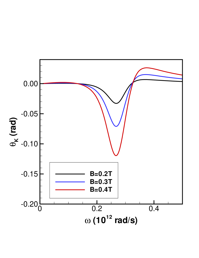
Figure 11: Kerr angle $\theta_{K}$ in the Voigt configuration as a function of frequency for $B_{0}=0.2,0.3,0.4$ T. Parameters: $n_{e}=0.25\times 10^{20}$ m^-3 and $\tau_{m}=10$ ps.

References

- (1) S. Bertrand, J.-M. Parent, R. Côté and I. Garate, Phys. Rev. B 100, 075107 (2019).
- (2) For a review of Weyl semimetals, see, for example : P. Hosur and X.-L. Qi, C. R. Physique 14, 857-870 (2013); N. P. Armitage, E. J. Mele, A. Vishwanath, Rev. Mod. Physics 90, 15001 (2018).
- (3) H. B. Nielsen and M. Ninomiya, Phys. Lett. B105, 219 (1981).
- (4) K.Y. Yang, Y.M. Lu, Y. Ran, Phys. Rev. B 84, 075129 (2011); G. Xu, H. Weng, Z. Wang, X. Dai, Z. Fang, Phys. Rev. Lett. 107, 186806 (2011); P. Goswami, S. Tewari, Phys. Rev. B 88, 245107 (2013); A.A. Burkov, L. Balents, Phys. Rev. Lett. 107, 127205 (2011); A.A. Zyuzin, S.Wu, A.A. Burkov, Phys. Rev. B 85, 165110 (2012).
- (5) J.H. Zhou, H. Jiang, Q. Niu, J.R. Shi, Chinese Phys. Lett. 30, 027101 (2013); Y. Chen, S. Wu, A.A. Burkov, Phys. Rev. B 88, 125105 (2013).
- (6) X. Wan, A.M. Turner, A. Vishwanath, S.Y. Savrasov, Phys. Rev. B 83, 205101 (2011); P. Hosur, Phys. Rev. B 86, 195102 (2012).
- (7) D. T. Son and B. Z. Spivak, Phys. Rev. B 88, 104412 (2013); H. Z. Lu, S. B. Zhang and S. Q. Shen, Phys. Rev. B 92, 045203 (2015); F. Wilczek, Phys. Rev. Lett. 58, 1799 (1987); A. A. Zyuzin and A. A. Burkov, Phys. Rev. B 86, 115133 (2012).
- (8) P. E. C. Ashby and J. P. Carbotte, Phys. Rev. 87, 245131 (2013); J. M. Shao and G. W. Yang, AIP advances 6, 025312 (2016); Y. Jiang, Z. Dun, S. Moon, H. Zhou, M. Koshino, D. Smirnov, and Z. Jiang, Nano Letters 18, 7726 (2018); X. Yuan, Z. Yan, C. Song, M. Zhang, Z. Li, C. Zhang, Y. Liu, W. Wang, M. Zhao, Z. Lin, T. Xie, J. Ludwig, Y. Jiang, X. Zhang, C. Shang, Z. Ye, J. Wang, F. Chen, Z. Xia, D. Smirnov, X. Chen, Z. Wang, H. Yan, and F. Xiu, Nature Communications 9 (2018).
- (9) P. E. C. Ashby and J. P. Carbotte, Phys. Rev. B 89, 245121 (2014); C. J. Tabert, J. P. Carbotte, and E. J. Nicol, Phys. Rev. B 93, 085426 (2016).
- (10) S. Tchoumakov, M. Civelli and M. O. Goerbig, Phys. Rev. Lett. 117, 086402 (2016).
- (11) I. Crassee, J. Levallois, A. L. Walter, M. Ostler, A. Bostwick, E. Rotenberg, T. Seyller, D. van der Marel and A. B. Kuzmenko, Nature Phys. 7, 48 (2011).
- (12) M. Kargarian, M. Randeria and N. Trivedi, Sci. Rep. 5, 12683 (2015).
- (13) S. Bertrand, I. Garate, and R. Côté, Phys. Rev. B 96, 075126 (2017).
- (14) K. Sonowal, A. Singh and A. Agarwal, Phys. Rev. B 100, 085436 (2019).
- (15) J. Yang, J. Kim and K.-S. Kim, Phys. Rev. B 98, 075203 (2018).
- (16) A. L. Levy, A. B. Sushkov, F. Liu, B. Shen, N. Ni, H. D. Drew and G. S. Jenkins, Phys. Rev. B 101, 125102 (2020).
- (17) B. Cheng, T. Schumann, S. Stemmer, and N. P. Armitage, arXiv:1910.13655 .
- (18) P. E. C. Ashby and J. P. Carbotte, Phys. Rev. B 87, 245131 (2013).
- (19) S. P. Mukherjee and J. P. Carbotte, Phys. Rev. B 96, 085114 (2017).
- (20) P. Goswami, J. H. Pixley, and S. Das Sarma, Phys. Rev. B 92, 075205 (2015).
- (21) H.-Z. Lu, S.-B. Zhang, and S. Q. Shen, Phys. Rev. B 92, 045203 (2015).
- (22) S. Das Sarma and E. H. Hwang, Phys. Rev. Lett. 102, 206412 (2009).
- (23) M. Balkanski and R. F. Wallis, Many-bopy aspects of solid state spectroscopy, North-Holland Physics Publishing, Amsterdam (1986).
- (24) C.-C. Lee et al., Phys. Rev. B 92, 235104 (2015).
- (25) D. Grassano, O. Pulci, A. M. Conte, and F. Bechstedt, Sci. Rep. 8, 3534 (2018).