Scheduling activities with time-dependent durations and resource consumptions

Abstract

In this paper we study time-dependent scheduling problems where activities consume a resource with limited availability. Activity durations as well as resource consumptions are assumed to be time-dependent and the resource can be replenished between activities. Because of the interaction of time-dependent activity durations and resource consumptions, scheduling policies based on starting all activities as early as possible may fail due to unnecessarily high resource consumptions. We propose a dynamic discretization discovery algorithm that generates a partially time-expanded network during the search. We propose preloading techniques allowing to significantly reduce the computational effort if the approach is embedded in an iterative solution procedure that frequently evaluates activity sequences that start with the same activities. We evaluate our approaches on a case of routing a fleet of electric vehicles in which vehicles can recharge batteries during the route.  
Keywords: time-dependent scheduling, resource constraints, break scheduling, preventive maintenance, electric vehicle routing

1 Introduction

Many operational activities consume some kind of resource throughout their execution. For example, engines used for executing activities consume energy. With the increasing replacement of internal combustion engines by battery electric propulsion systems, the limited battery capacity has to be considered when scheduling activities and it must be ensured that all activities can be executed without running out of energy (see, e.g., Pelletier et al. 2016). Similarly, the time required by a human operator can be seen as a resource that is consumed throughout the execution of activities and which is limited by work regulations (see, e.g., Federal Motor Carrier Safety Administration 2011, European Union 2003). Also machine times may be limited between preventive maintenance processes or inspection intervals, for example, aircrafts must be inspected before a total flight time of a given limit is reached (Legal Information Institute 2020).

In this paper we study the problem of scheduling a sequence of activities where activities consume a limited resource throughout execution. We assume that both activity durations and resource consumptions depend on the time of execution. A major cause of time-dependent activity durations and resource consumption is congestion, which can have a significant impact on the duration required to complete certain activities. In the 15 largest urban areas in the United States, for example, travel times on freeways are 44 percent higher during peak periods than during free flow times (Schrank et al. 2019). Similarly, in warehouses and manufacturing facilities, congestion can occur due to space limitations and narrow aisles (Zhang et al. 2009). Thus the time required for picking activities or moving a forklift may vary over the course of the day. Time-dependent durations may also occur for other reasons. For example, the total trip duration of a public transport user includes waiting time until the next scheduled departure and the actual travel time. Thus, the total trip duration depends on the time of the day and can be represented as time-dependent function (Rest and Hirsch 2016). In satellite imagery, as another example, the relative position of the satellite to an object on the earth surface depends on the position of the satellite in the orbit and the time required to tilt the satellite accordingly can be represented by a time-dependent function (Liu et al. 2017).

Time-dependent activity durations can have various ramifications that have received very little attention in the scientific literature. Consider, for example, the case of electric forklifts or vehicles. If activity durations and energy consumptions are time-dependent, the timing of the activities can be of particular importance in order to ensure that the total energy consumption of a sequence of activities stays below the total energy provided by the battery. Similarly, in the case of limited working times, the total working time of an operator may exceed the maximum working time allowed if most activities are conducted during peak-hours. Thus, activities may have to be shifted away from peak-hours in order not to exceed the legal limits on the working time. Therefore, the commonly used scheduling policy to schedule activities as early as possible may fail due to unnecessarily high resource consumptions.

Sometimes resources can be regenerated after they have been consumed. For example, an electric battery can be recharged, a human operator can take a rest as required by working regulations, or a maintenance process can reset the machine time available until the next maintenance is needed. In order to accommodate for such cases, we also study the problem of jointly scheduling activities and replenishments.

The contributions of this paper are: 1) we introduce the time-dependent activity scheduling problem with resource constraints; 2) we show that an optimal solution can easily be found if activity durations fulfil the the so-called first in first out (FIFO) property, i.e the property that an earlier start time implies an earlier or equal completion time, and resource consumption functions are non-decreasing in time; 3) we propose a dynamic discretization discovery algorithm for solving the problem in the more general case of non-monotonous consumption functions; 4) we extend the approach to the case where resources can be replenished between activities; 5) we propose an acceleration technique for iterative problem solving by preloading vertices of the partially expanded network obtained from a previous iteration; 6) we propose new benchmark instances for time-dependent vehicle routing with electric vehicles; 7) we evaluate the algorithms on these benchmark instances.

2 Related work

Resources that are consumed throughout the course of activities can be found in various scheduling problems. Often a capacity limit is given on such resources and the total consumption must not exceed the capacity. In the case where each activity has a constant resource consumption, the total resource consumption can easily be obtained by summing up the constants. This is for example the case in the capacitated vehicle routing problem (see, e.g., Irnich et al. 2014) where the maximum load of the vehicle can be interpreted as a resource that is depleted by the customer demands. In the multi-trip vehicle routing problem (see, e.g., Fleischmann 1990, Taillard et al. 1996, Cattaruzza et al. 2014), this full capacity of the resource can be restored when the vehicle returns to the depot. Schiffer et al. (2019) provide a recent review of vehicle routing problems in which vehicle routes include stops for replenishments, refueling, and breaks.

For route planning problems with battery-powered vehicles (see, e.g., Pelletier et al. 2016), the energy consumption of the vehicles depends on the distance travelled. Therefore, minimising route distances will help to create routes that can be conducted without running out of energy. Recharging the battery may be possible in order to increase the range of a vehicle. Schneider et al. (2014) study a vehicle routing problem in which electric vehicles can visit charging stations during the routes to recharge the battery. Unlike Schneider et al. (2014) who assume that the battery is always fully recharged, Felipe et al. (2014) allow to partially recharge the battery. Sweda et al. (2017) find optimal recharging policies for a given route determining when to recharge as well as the amount of energy charged. Montoya et al. (2017) consider non-linear charging functions and optimise where and which amount to charge. Baum et al. (2019) find optimal routes on road networks for a realistic distribution of charging stations as well as non-linear charging functions allowing partial recharging.

In the vehicle routing and truck driver scheduling problem (see, e.g., Tilk and Goel 2020, Goel and Vidal 2014, Prescott-Gagnon et al. 2010, Goel 2009), vehicle routes have to be generated in such a way that all customers can be visited within time windows and all routes can be executed without violating government regulations with respect to driving time limits. According to these regulations, truck drivers have to take breaks and rest periods at regular intervals. The remaining time without a break or rest period can be regarded as a resource that is consumed when driving. Although the driving time between two customers is assumed to be a given constant, time windows for customer visits may make it impossible to always drive as long as allowed by the regulations and only take breaks or rests when the legal driving time limits are reached. Instead, determining feasibility of each route requires the solution of a truck driver scheduling problem (see, e. g., Archetti and Savelsbergh 2009, Goel 2014; 2010, Goel and Kok 2012, Goel and Rousseau 2012, Goel et al. 2012). Minimising schedule durations is an even more complicated problem that is studied, for example, by Kok et al. (2011), Goel (2012b; c; a), and Rancourt et al. (2013).

Most of the above-mentioned studies assume that activity durations are given as constant values. In many real-life applications, however, the duration of activities depends on the time of the day. Scheduling problems with time-dependent processing times have been surveyed by Cheng et al. (2004) and Alidaee and Womer (1999). Vidal et al. (2015) review activity scheduling problems in which timing decisions are of particular importance and possibly time-dependent. Stecco et al. (2008) study a scheduling problem where setups with a time dependent duration are required between pairs of jobs and formulate the problem as a time-dependent traveling salesman problem. The time-dependent traveling salesman problem is also studied, e.g., by Nannicini et al. (2012), Montero et al. (2017), Cordeau et al. (2014), Taş et al. (2016). Vu et al. (2020) apply dynamic discretization discovery, originally proposed by Boland et al. (2017), for the time-dependent traveling salesman problem with time windows. Dynamic discretization discovery works on a time-expanded network, where only a small fraction of the vertices in the time-expanded networks is actually generated. For the case of arc costs which are non-decreasing in time, Vu et al. (2020) provide criteria allowing to prove optimality of a solution in the partially expanded network. He et al. (2019) also apply dynamic discretization discovery, but for the time-dependent shortest path problem. For the case of piecewise linear travel times satisfying the FIFO property, they propose an improvement of the dynamic discretization discovery based on an observation in Foschini et al. (2012) allowing to explore only a small fraction of breakpoints of the arc travel time functions.

A survey on vehicle routing problems with time-dependent travel times given by Gendreau et al. (2015). Dabia et al. (2013) present an exact approach for the time-dependent vehicle routing problem. Hashimoto et al. (2008) propose a method to determine an optimal time schedule for a route where travel times and costs are piecewise linear and lower semi-continuous time-dependent functions. Visser and Spliet (2020) show how ready time functions can be determined efficiently by composition of piecewise linear travel time functions.

The research concerning time-dependent activity duration and the consumption of limited resources which may have to be replenished is scarce. Drezet and Billaut (2008) analyse a project scheduling problem with time-dependent activity requirements and workers, which obey French workforce regulations and have various skill sets. A mixed-integer programing formulation and heuristic solution approaches are presented. For home health care, Rest and Hirsch (2016) present a scheduling approach considering break requirements for healthcare personnel assuming that staff members use a combination of walking and public transport. Travel times with public transport are modelled as time-dependent functions, where staff members may have to wait for the next tram, train, or metro. The scheduling of breaks is conducted based on heuristic rules. Kok et al. (2011) present a mixed-integer program for the problem of finding a schedule of minimal duration for a truck driver who must take breaks as required by European Union regulations. The problem is extended by time-dependent travel times and used as a subproblem for route evaluations within an insertion heuristic. The subproblem is solved with a general purpose mixed-integer programming solver. Kleff (2019) studies the problem of finding a time-dependent shortest path from an origin to a destination in which breaks can be taken at parking lots in the network. The driving time is limited by European Union regulations. An approach combining forward exploration from the origin to a parking lot and backwards exploration from the destination to a parking is presented.

3 Problem description

Let us consider a sequence of activities $(1,2,\ldots,n)$ to be conducted in the given order and without preemption. The time-dependent duration and resource consumption of each activity $i$ are given by functions $\tau_{i}(t_{i})$ and $\rho_{i}(t_{i})$, respectively, where $t_{i}$ refers to the start time of the activity. Each activity $i$ must start within a given time interval $[e_{i},l_{i}]$ and the cumulative resource consumption must not exceed a given quantity $Q$. With $\theta_{i}(t_{i})=t_{i}+\tau_{i}(t_{i})$ for all $i\in\{1,...,n\}$, the time-dependent activity scheduling problem (TDASP) can be represented by

minimise

$$\theta_{n}(t_{n})$$ (1)

subject to

$$\theta_{i}(t_{i})\leq t_{i+1}\textrm{ for all }1\leq i<n$$ (2)

$$\sum_{i=1}^{n}\rho_{i}(t_{i})\leq Q$$ (3)

$$t_{i}\in[e_{i},l_{i}]\textrm{ for all }1\leq i\leq n$$ (4)

The objective (1) is to minimise the completion time. Constraint (2) demands that the start time of any activity must not be before the completion time of the previous activity. Constraint (3) requires that the cumulative resource consumption does not exceed the available amount. Lastly, the domain of the variables is given by (4).

Throughout this paper we assume that the completion time functions $\theta_{i}(\cdot)$ are non-decreasing for all $i\in\{1,...,n\}$, meaning that completion times satisfy the FIFO property. Without loss of generality we assume in the remainder of this paper that time windows are restricted in such a way that $\theta_{i}(e_{i})\leq e_{i+1}$ and $\theta_{i}(l_{i})\leq l_{i+1}$ for all $1\leq i<n$.

Lemma 1

Assume we have a sequence $t_{1},t_{2},\ldots,t_{n}$ with $t_{1}=e_{1}$ and $t_{i}=\max\{\theta_{i-1}(t_{i-1}),e_{i}\}$ for each $1<i\leq n$. If $\rho_{i}(\cdot)$ is non-decreasing for $1\leq i\leq n$ and constraints (2) to (4) are satisfied, then $t_{1},t_{2},\ldots,t_{n}$ is an optimal solution of the TDASP. If any of the constraints (2) to (4) is violated no feasible solution exists.

Proof.

As the completion time functions $\theta_{i}(\cdot)$ are non-decreasing by the FIFO property, the proof is trivial for non-decreasing resource consumption functions $\rho_{i}(\cdot)$. ∎

Resource consumption functions can be non-decreasing in scheduling problems with deterioration (see, e.g., Mosheiov 1994). However, in other cases, the resource consumption may, e.g., depend on congestion levels and vary throughout the day. In such cases it may be possible to reduce the total resource consumption by delaying the start time of some of the activities. In the following sections we present solution approaches for cases in which resource consumption functions are not monotonous.

3.1 Time-expanded networks

An approximation of the solution of the TDASP can be obtained by discretising time and modelling the problem as a time-expanded network. Let us assume we are given a parameter $\varepsilon>0$ for which $e_{i}$ and $l_{i}$ are a multiple of $\varepsilon$ for each activity $i$. Then, we can create for each activity $i$ and each time point $t_{i}\in\{e_{i},e_{i}+\varepsilon,\ldots,l_{i}\}$ a vertex $(i,t_{i})$ in the time-expanded network. The edges of the time-expanded network are obtained by connecting every vertex $(i,t_{i})$ with vertex $(i+1,t_{i+1})$ if and only if $t_{i+1}\geq\theta_{i}(t_{i})$. Figure 1 illustrates such a time-expanded network with vertex sets $V_{i}$ for each $1\leq i\leq n$.

Figure 1: A time-expanded network

When setting $q_{(i,t)}=\rho_{i}(t)$ for all $(i,t)\in V=\bigcup_{i=1}^{n}V_{i}$, we can solve the TDASP by calling the function ${\tt solve}\big{(}V,\left(q_{(i,t)}\right)_{(i,t)\in V}\big{)}$ shown in Algorithm 1. Note, that we could have simply used $\rho_{i}(t)$ instead of $q_{(i,t)}$ in the algorithm, however, the used notation allows us in the following sections to use different values of $q_{(i,t)}$ to accelerate the search.

Data: $(e_{i},l_{i},\tau_{i},\theta_{i},\rho_{i})_{i\in\{1,\ldots,n\}},Q$

1 Function ${\tt TEN\!::\!solve}\big{(}V,\left(q_{(i,t)}\right)_{(i,t)\in V}\big{)}$

2       $\bar{V}\leftarrow\emptyset$;

3       foreach $(i,t)\in V$ do

4             $\ell_{(i,t)}\leftarrow\left\{\begin{array}[]{ll}0&\textrm{ if }i=1\\ \infty&\textrm{ else }\end{array}\right.$;

5            

6       end foreach

7      while  exists $(i,t)\in V\setminus\bar{V}$ with $\ell_{(i,t)}+q_{(i,t)}\leq Q$ do

8             $(i,t)\leftarrow\displaystyle\operatorname*{{argmin^{\it lex}}}_{(i,t)\in V\setminus\bar{V}:\ell_{(i,t)}+q_{(i,t)}\leq Q}\Big{\{}\big{(}\theta_{i}(t)+\sum_{j=i+1}^{n}\min_{t^{\prime}\in[e_{j},l_{j}]}\tau_{j}(t^{\prime}),\ i,t\big{)}\Big{\}}$;

9             $\bar{V}\leftarrow\bar{V}\cup\{(i,t)\}$;

10             if  $i=n$  then break ;

11             foreach $t^{\prime}\in\{t^{\prime}\mid(i+1,t^{\prime})\in V\setminus\bar{V},\theta_{i}(t)\leq t^{\prime}\}$ do

12                   if  $\ell_{(i,t)}+q_{(i,t)}<\ell_{(i+1,t^{\prime})}$  then

13                         $\ell_{(i+1,t^{\prime})}\leftarrow\ell_{(i,t)}+q_{(i,t)}$;

14                         $p_{(i+1,t^{\prime})}\leftarrow(i,t)$

15                   end if

16                  

17             end foreach

18            

19       end while

20      return ${\tt solution}\big{(}\bar{V},\left(q_{v},\ell_{v},p_{v}\right)_{v\in\bar{V}}\big{)}$;

21      

22 end

Algorithm 1 Solving the TDASP in a time-expanded network

The algorithm is similar to an A*-Algorithm for shortest path problems (Hart et al. 1968). However, labels are not related to objective function values. Instead, labels indicate the cumulative resource consumption until the start of each activity at a particular time. The algorithm starts with initializing a set of vertices $\bar{V}$ for which the label is permanently set. It tentatively sets all labels associated to the first activity to zero, and all other labels to infinity. As long as there is a vertex in $V\setminus\bar{V}$ which has a label allowing to conduct the activity without exceeding the capacity, the algorithm selects such a vertex $(i,t)\in V\setminus\bar{V}$ according to a lexicographical ordering on the lower bound on the completion time of the last activity, the activity index, and the time associated to the vertex. The lexicographical ordering is necessary to ensure that all relevant predecessors are considered before selecting a vertex. The selected vertex is inserted in $\bar{V}$. If the selected vertex belongs to the last activity, the algorithm terminates. Otherwise, non-permanent labels of the next activity are updated if their value can be reduced. Whenever a label is updated, the predecessor $p_{v}$ for the vertex is updated so that the solution can be reconstructed by a function ${\tt solution}\big{(}\bar{V},\left(q_{v},\ell_{v},p_{v}\right)_{v\in\bar{V}}\big{)}$. If a solution is found, this function returns the vertices of the solution obtained by selecting the earliest vertex $(n,t)$ with $\ell_{(n,t)}+q_{(n,t)}\leq Q$ and iterating through its predecessors. If no solution is found, the function returns $\big{\{}(1,\infty),\ldots,(n,\infty)\big{\}}$. For brevity reasons we omit a detailed description of this trivial function.

Lemma 2

Algorithm 1 finds an optimal solution of the TDASP restricted to the time-expanded network with vertex set $V$ if and only if such a solution exists.

Proof.

Assume that vertex $(i,t)$ is selected in an iteration of the algorithm. Due to the FIFO property, each potential predecessor of $(i,t)$ must have been selected in an earlier iteration. Thus, $\ell_{(i,t)}$ represents the minimal cumulative resource consumption before conducting activity $i$ at time $t$. If $(n,t)$ is selected and $\ell_{(n,t)}+q_{(n,t)}\leq Q$, then $t$ is the earliest time for which $\ell_{(n,t)}+q_{(n,t)}\leq Q$. Thus, the solution obtained by backtracking the predecessors is optimal. If the algorithm terminates without having selected a vertex $(n,t)$ with $\ell_{(n,t)}+q_{(n,t)}\leq Q$, then there is no path $(1,t_{1}),\ldots,(n,t_{n})$ with $(i,t_{i})\in V$ for $i\in\{{1},\ldots,{n}\}$, $\theta_{i}(t_{i})\leq t_{i+1}$ for $i\in\{{1},\ldots,{n-1}\}$, and $\sum_{i=1}^{n}q_{(i,t_{i})}\leq Q$. ∎

3.2 Dynamic Discretization Discovery

The difficulty in solving the TDASP with discretized times is that the number of vertices in the time-expanded network can become very large for small values of $\varepsilon$, i.e. the parameter influencing the granularity of the time discretization. In order to reduce the number of vertices we now show how to solve the TDASP with discretized times on a partially expanded network similar to the dynamic discretization discovery approach by Vu et al. (2020) for the time-dependent traveling salesman problem with time windows. Unlike Vu et al. (2020), who assume that arc costs are non-decreasing in time, we assume that resource consumption functions can be non-monotonous.

In the remainder of this section we will refer to a partially expanded network if the set of vertices $V$ is a subset of the vertices of the fully expanded network and the set of edges is obtained by connecting every vertex $(i,t_{i})$ with vertex $(i+1,t_{i+1})$ if and only if $t_{i+1}\geq\theta_{i}(t_{i})$. Our approach will generate and modify such partially expanded networks with the following properties.

Property 1

For each $1\leq i\leq n$ we have $(i,e_{i})\in V$ and $(i,l_{i})\in V$.

Property 2

For each vertex $(i,t)\in V$ with $e_{i+1}<\varepsilon\left\lceil\frac{\theta_{i}(t)}{\varepsilon}\right\rceil<l_{i+1}$, we have $\Big{(}i+1,\varepsilon\left\lceil\frac{\theta_{i}(t)}{\varepsilon}\right\rceil\Big{)}\in V$.

Property 3

Each vertex $(i,t)\in V$ with $t<l_{i}$ is assigned a consumption value of

$$q_{(i,t)}=\min_{\bar{t}\in\{t,t+\varepsilon,\ldots,t^{\prime}-\varepsilon\}}\rho_{i}(\bar{t})$$

where $t^{\prime}>t$ is the smallest value for which $(i,t^{\prime})\in V$. Each vertex $(i,l_{i})\in V$ is assigned a consumption value of $q_{(i,l_{i})}=\rho_{i}(l_{i})$.

Property 1 guarantees that for each activity $i$, a vertex representing the earliest and latest start time is included in the partially expanded network. For every vertex, its immediate successor is included in the partially expanded network if Property 2 is satisfied. Because of Property 3, each vertex $(i,t)$ is assigned a value $q_{(i,t)}$, which is a lower bound on the actual resource consumption of the activity for any start time between $t$ and $t^{\prime}-\varepsilon$, where $t^{\prime}$ refers to the next vertex of activity $i$.

With these properties we can make the following observation.

Lemma 3

The optimal solution of a TDASP restricted to a partially expanded network satisfying Properties 1 to 3 is a lower bound on the optimal solution of the fully expanded TDASP with discretized times.

Proof.

Assume that vertices $(1,t_{1}),$ $\ldots,(n,t_{n})$ correspond to an optimal solution of the fully expanded TDASP with discretized times. Because of Properties 1 and 2, we can find a path $(1,t^{\prime}_{1}),$ $\ldots,(n,t^{\prime}_{n})$ in the partially expanded network, where for each $1\leq i\leq n$ the value $t^{\prime}_{i}$ is the largest while not exceeding $t_{i}$ such that $(i,t^{\prime}_{i})$ is in the partially expanded network. Because of Property 3, we have $q_{(i,t^{\prime}_{i})}\leq\rho_{i}(t_{i})$ for each $1\leq i\leq n$ and $\sum_{i=1}^{n}q_{(i,t^{\prime}_{i})}\leq\sum_{i=1}^{n}\rho_{i}(t_{i})\leq Q$. Therefore, $(1,t^{\prime}_{1}),$ $\ldots,(n,t^{\prime}_{n})$ is feasible for the TDASP restricted to the partially expanded network and has a completion time that is smaller or equal to the solution of the fully expanded TDASP with discretized times. ∎

Lemma 4

Assume that the path $(1,t_{1}),$ $\ldots,(n,t_{n})$ corresponds to an optimal solution of the TDASP restricted to a partially expanded network satisfying Properties 1 to 3. Furthermore, assume that $q_{(i,t_{i})}=\rho_{i}(t_{i})$ for each $1\leq i\leq n$. Then, the path corresponds to an optimal solution of the fully expanded TDASP with discretized times.

Proof.

If $q_{(i,t_{i})}=\rho_{i}(t_{i})$ for each $1\leq i\leq n$, then $\sum_{i=1}^{n}\rho_{i}(t_{i})=\sum_{i=1}^{n}q_{(i,t_{i})}\leq Q$. Therefore, $(1,t_{1}),$ $\ldots,(n,t_{n})$ is feasible for the TDASP with discretized times. Because of Lemma 3 we can conclude that the path corresponds to an optimal solution of the TDASP with discretized times. ∎

Data: $(e_{i},l_{i},\tau_{i},\theta_{i},\rho_{i})_{i\in\{1,\ldots,n\}},Q,\varepsilon$

1 Function ${\tt DDD\!::\!initialise}()$

2       $V\leftarrow\emptyset$;

3       for $i\leftarrow n$ to $1$ do

4             $\big{(}V,(q_{v})_{v\in V}\big{)}\leftarrow{\tt DDD\!::\!addRecursive}\big{(}V,(q_{v})_{v\in V},(i,l_{i})\big{)}$;

5             $\big{(}V,(q_{v})_{v\in V}\big{)}\leftarrow{\tt DDD\!::\!addRecursive}\big{(}V,(q_{v})_{v\in V},(i,e_{i})\big{)}$;

6            

7       end for

8      return $\big{(}V,(q_{v})_{v\in V}\big{)}$;

9      

10 end

11Function ${\tt DDD\!::\!addRecursive}\big{(}V,(q_{v})_{v\in V},(i,t)\big{)}$

12       if $(i,t)\in V$ then  return $\big{(}V,(q_{v})_{v\in V}\big{)}$ ;

13       $V\leftarrow V\cup\{(i,t)\}$;

14       if $t=l_{i}$ then

15             $q_{(i,t)}\leftarrow\rho_{i}(t)$

16       else

17             $t^{\prime}\leftarrow\min\{t^{\prime}\mid(i,t^{\prime})\in V,t^{\prime}>t\}$;

18             $q_{(i,t)}\leftarrow\displaystyle\min_{\bar{t}\in\{t,t+\varepsilon,\ldots,t^{\prime}-\varepsilon\}}\rho_{i}(\bar{t})$;

19             if $t>e_{i}$ then

20                   $t^{\prime}\leftarrow\max\{t^{\prime}\mid(i,t^{\prime})\in V,t^{\prime}<t\}$;

21                   $q_{(i,t^{\prime})}\leftarrow\displaystyle\min_{\bar{t}\in\{t^{\prime},t^{\prime}+\varepsilon,\ldots,t-\varepsilon\}}\rho_{i}(\bar{t})$;

22                  

23             end if

24            

25       end if

26      if $i=n$ then

27             return $\big{(}V,(q_{v})_{v\in V}\big{)}$

28       else

29             return ${\tt DDD\!::\!addRecursive}\Big{(}V,(q_{v})_{v\in V},\big{(}i+1,\max\{e_{i+1},\varepsilon\big{\lceil}\frac{\theta_{i}(t)}{\varepsilon}\big{\rceil}\}\big{)}\Big{)}$

30       end if

31      

32 end

33

Algorithm 2 Initialising a partial time-expanded network

We can use Algorithm 2 to create an initial partially expanded network. According to Property 1, the algorithm adds vertices corresponding to each activity at the start and end of the time window. These vertices are added in the order $(n,l_{n}),(n,e_{n}),\ldots,(1,l_{1}),(1,e_{1})$ and their immediate successors are recursively added according to Property 2. When adding a vertex $(i,t)$ the consumption values of the new vertex and the preceding vertex $(i,t^{\prime})$ are set as required by Property 3.

Data: $(e_{i},l_{i},\tau_{i},\theta_{i},\rho_{i})_{i\in\{1,\ldots,n\}},Q,\varepsilon$

1 Function ${\tt DDD\!::\!solve}()$

2       $\big{(}V,(q_{v})_{v\in V}\big{)}\leftarrow{\tt DDD\!::\!initialise}()$;

3       repeat

4             $\big{\{}(1,t_{1}),\ldots,(n,t_{n})\big{\}}={\tt TEN\!::\!solve}\big{(}V,(q_{v})_{v\in V}\big{)}$;

5             if  $t_{n}=\infty$ then break;

6             if  exists $1\leq i\leq n$ with $\rho_{i}(t_{i})>q_{(i,t_{i})}$ then

7                   select $(i,t_{i})$ with $\rho_{i}(t_{i})>q_{(i,t_{i})}$;

8                   $t\leftarrow\min\{t^{\prime}\mid t^{\prime}>t_{i},(i,t^{\prime})\in V\}$;

9                   repeat

10                         $t\leftarrow\varepsilon\lceil\frac{t_{i}+t}{2\varepsilon}\rceil$;

11                        

12                  until $\displaystyle\min_{\bar{t}\in\{t_{i},t_{i}+\varepsilon,\ldots,t-\varepsilon\}}\rho_{i}(\bar{t})>q_{(i,t_{i})}$;

13                  $\big{(}V,(q_{v})_{v\in V}\big{)}\leftarrow{\tt DDD\!::\!addRecursive}\big{(}V,(q_{v})_{v\in V},(i,t)\big{)}$;

14                  

15             end if

16            

17      until $\rho_{i}(t_{i})=q_{(i,t_{i})}\textrm{ for all }1\leq i\leq n$;

18      return $\big{\{}(1,t_{1}),\ldots,(n,t_{n})\big{\}}$;

19      

20 end

21

Algorithm 3 Dynamic discretization discovery algorithm

Algorithm 3 solves the TDASP with discretized times by dynamically creating a time-expanded network. The algorithm starts by initialising the network using Algorithm 2. Then it iterates until a solution of the TDASP with discretized times is found. Each iteration begins with finding a solution of the TDASP restricted to the partially expanded network using Algorithm 1. If there is an activity $i$ in the solution that begins at a time $t$ such that $\rho_{i}(t)>q_{(i,t)}$, then the total consumption associated with the solution may exceed the capacity. Therefore, a new vertex is added to the partially expanded network between $(i,t)$ and the next vertex of activity $i$. The time for the new vertex is selected in such a way that the value of $q_{(i,t_{i})}$ is increased when adding the new vertex.

If a feasible solution exists, the algorithm either terminates with the optimal solution, or adds at least one vertex to the partially expanded network in each iteration. Therefore, the algorithm is guaranteed to terminate with the optimal solution. In the worst case, the algorithm may have to fully expand the network. However, in general, the algorithm can be expected to require only a fraction of the vertices.

4 Replenishments

So far we assumed that the resource cannot be used after it has been consumed by the activities. This is the case, for example, if electric batteries cannot be recharged or if maximum working hours or operating times are reached. In many cases, however the resource can be regenerated. For example, electric batteries can be recharged, workers are allowed to work again after taking a sufficiently long break, or machines can be used again after some maintenance has been conducted. In this section we consider an extension of the TDASP in which the resource can be replenished between the end of an activity and the begin of the next activity. We assume that the time required to fully replenish a resource after conducting activity $i$ can be determined by a consumption-dependent and non-decreasing replenishment function $\Delta_{i}(Q_{i})$, where $Q_{i}$ is the cumulative resource consumption after completing activity $i$.

The resulting time-dependent activity scheduling problem with replenishments (TDASPR) is to

minimise

$$\theta_{n}(t_{n})$$ (5)

subject to

$$\theta_{i}(t_{i})+y_{i}\Delta_{i}(Q_{i})\leq t_{i+1}\textrm{ for all }1\leq i<n$$ (6)

$$Q_{1}=\rho_{1}(t_{1})$$ (7)

$$Q_{i+1}=(1-y_{i})Q_{i}+\rho_{i+1}(t_{i+1})\textrm{ for all }1\leq i<n$$ (8)

$$t_{i}\in[e_{i},l_{i}],Q_{i}\in[0,Q],y_{i}\in\{0,1\}\textrm{ for all }1\leq i\leq n.$$ (9)

In this problem $Q_{i}$ is a variable representing the cumulative resource consumption between the last replenishment and completion of activity $i$, and $y_{i}$ is a binary variable representing whether the resource is replenished after conducting activity $i$. The objective function is the same as in the case without replenishments. Constraint (6) is analogous to Constraint (2) but includes the replenishment duration if necessary. Constraints (7) and (8) ensure that the cumulative resource consumption is correctly determined and Constraints (9) restricts the domains of the variables.

The special case where replenishments must or must not be taken after some of the activities is covered in Appendix B.

4.1 Replenishments in time-expanded networks

In the following we show how dynamic discretization discovery can be used to solve the TDASPR. For this, we replace Algorithm 1 by Algorithm 4 which dynamically adds new vertices corresponding to a fully replenished resource to the partially expanded network.

Data: $(e_{i},l_{i},\tau_{i},\theta_{i},\rho_{i},\Delta_{i})_{i\in\{1,\ldots,n\}},Q,\varepsilon$

1 Function ${\tt TEN}{\hbox{-}}\Delta{\tt::\!solve}\big{(}V,\left(q_{(i,t)}\right)_{(i,t)\in V}\big{)}$

2       $\bar{V}\leftarrow\emptyset$;

3       foreach $(i,t)\in V$ do

4             $\ell_{(i,t)}\leftarrow\left\{\begin{array}[]{ll}0&\textrm{ if }i=1\\ \infty&\textrm{ else }\end{array}\right.$;

5            

6       end foreach

7      while  exists $(i,t)\in V\setminus\bar{V}$ with $\ell_{(i,t)}+q_{(i,t)}\leq Q$ do

8             $(i,t)\leftarrow\displaystyle\operatorname*{{argmin^{\it lex}}}_{(i,t)\in V\setminus\bar{V}:\ell_{(i,t)}+q_{(i,t)}\leq Q}\Big{\{}\big{(}\theta_{i}(t)+\sum_{j=i+1}^{n}\min_{t^{\prime}\in[e_{j},l_{j}]}\tau_{j}(t^{\prime}),\ i,t\big{)}\Big{\}}$;

9             $\bar{V}\leftarrow\bar{V}\cup\{(i,t)\}$;

10             if  $i=n$  then break ;

11             $t^{*}\leftarrow\varepsilon\big{\lceil}\frac{\theta_{i}(t)+\Delta_{i}(\ell_{(i,t)}+q_{(i,t)})}{\varepsilon}\big{\rceil}$;

12             if  $t^{*}\leq l_{i+1}$  then

13                   ${\tt DDD\!::\!addRecursive}\big{(}V,(q_{v})_{v\in V},(i+1,t^{*}))$

14             end if

15            foreach $t^{\prime}\in\{t^{\prime}\mid(i+1,t^{\prime})\in V\setminus\bar{V},\theta_{i}(t)\leq t^{\prime}<t^{*}\}$ do

16                   if  $\ell_{(i,t)}+q_{(i,t)}<\ell_{(i+1,t^{\prime})}$  then

17                         $\ell_{(i+1,t^{\prime})}\leftarrow\ell_{(i,t)}+q_{(i,t)}$;

18                         $p_{(i+1,t^{\prime})}\leftarrow(i,t)$

19                   end if

20                  

21             end foreach

22             foreach $t^{\prime}\in\{t^{\prime}\mid(i+1,t^{\prime})\in V\setminus\bar{V},t^{\prime}\geq t^{*}\}$ do

23                   $\ell_{(i+1,t^{\prime})}\leftarrow 0$;

24                   $p_{(i+1,t^{\prime})}\leftarrow(i,t)$

25             end foreach

26            

27       end while

28      return ${\tt solution}\big{(}\bar{V},\left(q_{v},\ell_{v},p_{v}\right)_{v\in\bar{V}}\big{)}$;

29      

30 end

Algorithm 4 Solving the TDASPR in a partially expanded network

Whenever a vertex $(i,t)$ with $i<n$ is selected in Algorithm 4, the algorithm determines the earliest replenishment time $t^{*}$ after conducting activity $i$ at time $t$. If $t^{*}\leq l_{i+1}$, the vertex $(i+1,t^{*})$ is added to $V$ using algorithm ${\tt DDD\!::\!addRecursive}$. Then, all labels for vertices with a time prior to $t^{*}$ are updated if their value can be reduced and all labels for vertices with a later time are set to zero.

Lemma 5

Assume that Algorithm 4 is applied to a partially expanded network satisfying Properties 1 to 3. Then, the solution of the algorithm is a lower bound on the solution in the fully expanded network.

Proof.

Let us first note that the solution returned by Algorithm 4 is the same as the solution returned by Algorithm 4 without Line 4. For the ease of argumentation, we therefore base our proof on a variant of Algorithm 4 without Line 4. Let $(1,t_{1}),$ $\ldots,(n,t_{n})$ denote an optimal solution in the fully expanded network. Let $\bar{V}$ denote the set of permanently labelled vertices after execution of this variant of the algorithm, including the vertices that may have been added to $V$ during the course of the algorithm. Let $(1,\bar{t}_{1}),$ $\ldots,(n,\bar{t}_{n})\in\bar{V}$ denote the vertices returned by the algorithm. Analogously to Lemma 2 we can show that $\bar{t}_{n}$ is smaller or equal to the completion time of any other path through vertices in $\bar{V}$ not exceeding the capacity between replenishments.

Let $(1,t^{\prime}_{1}),$ $\ldots,(n,t_{n}^{\prime})$ denote the vertices in $\bar{V}$ for which $t^{\prime}_{i}$ is the largest time not exceeding $t_{i}$ for each $i\in\{{1},\ldots,{n}\}$. These vertices can be found because of Property 1. As $\theta_{i}$ is non-decreasing for each $i\in\{{1},\ldots,{n}\}$, Property 2 guarantees that $\theta_{i}(t^{\prime}_{i})\leq t^{\prime}_{i+1}$ for $i\in\{{1},\ldots,{n-1}\}$.

Assume, that in the optimal solution $(1,t_{1}),$ $\ldots,(n,t_{n})$, the first replenishment is conducted just before starting activity $j$. Because of Property 3, we have $\sum_{i=1}^{j-1}q_{(i,t^{\prime}_{i})}\leq\sum_{i=1}^{j-1}\rho_{i}(t_{i})\leq Q$. Because $\Delta_{j-1}$ is non-decreasing, we have $\theta_{j-1}(t^{\prime}_{j-1})+\Delta_{j-1}\big{(}\sum_{i=1}^{j-1}q_{(i,t^{\prime}_{i})}\big{)}\leq\theta_{j-1}(t_{j-1})+\Delta_{j-1}\big{(}\sum_{i=1}^{j-1}\rho_{i}(t_{i})\big{)}$. Therefore, there is a vertex $(j,t)\in\bar{V}$ with $t\leq t_{j}$ and $\ell_{(j,t)}=0$. By definition we have $t\leq t^{\prime}_{j}\leq t_{j}$ and we can conclude that $\ell_{(j,t^{\prime}_{j})}=0$. Analogously we can show that $\sum_{i=j}^{k-1}q_{(i,t^{\prime}_{i})}\leq\sum_{i=j}^{k-1}\rho_{i}(t_{i})\leq Q$ and $\ell_{(k,t^{\prime}_{k})}=0$ if the next replenishment in the solution $(1,t_{1}),$ $\ldots,(n,t_{n})$ is conducted just before starting activity $k$. We can apply this argument repeatedly to conclude that the capacity is not exceeded along the path $(1,t^{\prime}_{1}),$ $\ldots,(n,t^{\prime}_{n})$ and that $\ell_{(n,t^{\prime}_{n})}+q_{(n,t^{\prime}_{n})}\leq Q$. Thus, $\bar{t}_{n}\leq t^{\prime}_{n}\leq t_{n}$. ∎

Lemma 6

Assume that the path $(1,t_{1}),$ $\ldots,(n,t_{n})$ corresponds to a solution created by Algorithm 3 using Algorithm 4. Furthermore, assume that $q_{(i,t_{i})}=\rho_{i}(t_{i})$ for each $1\leq i\leq n$. Then, the path corresponds to an optimal solution of the fully expanded TDASPR with discretized times.

Proof.

For each $1\leq i\leq n$ let $\ell_{(i,t_{i})}$ denote the corresponding label created by the algorithm. Let $i$ be any activity index with $\ell_{(i,t_{i})}=0$. For any activity index $j>i$ such that no replenishment is conducted between $i$ and $j$, we have $Q\geq\ell_{(j,t_{j})}+q_{(j,t_{j})}=\sum_{k=i}^{j}q_{(k,t_{k})}=\sum_{k=i}^{j}\rho_{k}(t_{k})$. Therefore, the duration of any replenishment is sufficiently long and the capacity is never exceeded between replenishments. Thus, $(1,t_{1}),$ $\ldots,(n,t_{n})$ is a feasible path in the fully expanded network. Because of Lemma 5 we can conclude that the path corresponds to an optimal solution of the TDASP with discretized times. ∎

5 Preloading of vertices

Assume we have already solved the problem for a sequence of activities $(1,\ldots,n)$ and we want to solve the problem for a sequence $(1,\ldots,n,n+1,\ldots,m)$. It is likely that some of the vertices that are generated when scheduling activities $(1,\ldots,n)$ are also generated when scheduling activities $(1,\ldots,n,n+1,\ldots,m)$. We can reduce the computational effort associated to finding such vertices again by preloading them before starting the solution process for sequence $(1,\ldots,n,n+1,\ldots,m)$. On the other hand, preloading all of the vertices generated when determining a schedule for activities $(1,\ldots,n)$ may create an unnecessary computational overhead, because only a share of the vertices can be expected to be required to find a solution for activities $(1,\ldots,n,n+1,\ldots,m)$.

To balance the tradeoff between salvaging previous computational effort and avoiding unnecessary overhead by adding too many vertices, we propose to preload all vertices of the solution path for sequence $(1,\ldots,n)$ to our partially expanded network after initialization and before starting the solution process. In order to ensure that $q_{(i,t)}=\rho_{i}(t)$ for all vertices preloaded, we also add the immediate successors. As all vertices are added using the function ${\tt DDD\!::\!addRecursive}$, Properties 1 to 3 maintain satisfied. Consequently, the optimality conditions for all vertices on the previous solution path are satisfied.

The benefit of adding these vertices after initialization of the partially expanded network is that the total number of vertices generated by the dynamic discretization discovery may be drastically reduced for those cases where the solution for sequence $(1,\ldots,n,n+1,\ldots,m)$ overlaps with the solution for sequence $(1,\ldots,n)$. In some cases, however, preloading may cause a small overhead because vertices may be recursively added that are not needed for the solution process.

6 Evaluation

This paper is motivated by an industry project on last-mile deliveries with electric vehicles, where a homogeneous fleet of electric delivery vehicles is used to deliver parcels within metropolitan areas, i.e., regions consisting of densely populated city centres and less-populated surrounding territories. Traffic conditions depend both on the particular area as well as the time of the day with morning and afternoon peak hours. With increasing distance to the city centres, the impact of peak hours on travel times decreases. Thus, the time-dependency of travel times is not homogeneous and delays caused by congestion can be avoided by circumventing city centres during peak hours. Current electric vehicles have minimal consumption per unit distance at moderate speeds while the consumption increases towards very low or high velocities. Therefore, the energy consumption of the vehicles is related to travel speeds, which in turn depend on the congestion level. All vehicles leave the depot fully charged and have to return to the depot before running out of energy. They can recharge the battery at the depot as well as at public charging infrastructure.

Due to confidentiality reasons, we are not allowed to evaluate our approaches on instances obtained from data of our project partners. Therefore, we generate artificial instances for the time-dependent vehicle routing problem with replenishments having the characteristics described above. Our instances are based on the well-known instances for the vehicle routing problem with time windows by Solomon (1987). These instances have customer locations distributed in the Euclidean plane and are subdivided into instance sets with clustered customer locations (C1 and C2), randomly distributed customer locations (R1 and R2), and mixed locations (RC1 and RC2).

Figure 2: Time-dependent congestion $\delta(t)$

In order to include time-dependent travel times, we introduce a time-dependent congestion factor $\delta(t)\in[0,1]$ for each point in time as shown in Figure 2. The time values on the horizontal axis in the figure are given relative to the duration of the time horizon which differs throughout the instances. Low levels of $\delta(t)$ indicate free-flow traffic conditions during off-peak hours. High values of $\delta(t)$ indicate high congestion levels during morning and afternoon peak-hours.

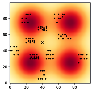
(a) C1 instances

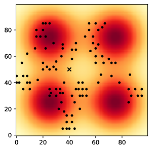
(b) C2 instances

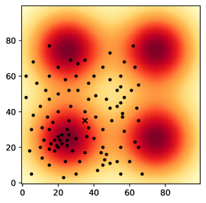
(c) R1 & R2 instances

(d) RC1 & RC2 instances

Figure 3: Location-dependent congestion $\gamma(x,y)$ and customer locations.

We assume a city centre in each quadrant of the Euclidean plane where congestion is maximal. In order to consider that the level of congestion decreases with increasing distance to the city centres, we calculate a location-dependent congestion factor $\gamma(x,y)\in[0,1]$ by the Gaussian function based on the distance to the city centres. Figure 3 shows the location-dependent congestion factors, the customer locations (shown as $\bullet$), and the location of the depot (shown as $\times$) for the different subsets of instances proposed by Solomon (1987). Low values of $\gamma(x,y)$ indicate low sensitivity to congestion and are illustrated in light color. High values of $\gamma(x,y)$ indicate high sensitivity to congestion and are illustrated in dark color. We can see that all instances comprise customers located in areas prone to congestion and others in areas where congestion is negligible. Even if two customers are located in areas without significant congestion, the direct path from one to the other may traverse congested areas during peak-hours.

For each integer valued point $(x,y)$, we calculate the time required to travel a unit distance at a time $t$ by

$$\tau_{(x,y)}(t)=\frac{\tau_{(x,y)}^{\mathrm{free}}}{1-\min\big{\{}0.8,\gamma(x,y)\big{\}}\cdot\delta(t)},$$ (10)

where $\tau_{(x,y)}^{\mathrm{free}}$ is the congestion-agnostic time necessary to travel a unit distance at point ${(x,y)}$. The factor $\min\big{\{}0.8,\gamma(x,y)\big{\}}$ in (10) is used to generate homogeneous travel times in an area around the city centres. The maximum travel time close to a city centre is five times the free flow travel time.

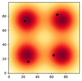
(a) One station per city

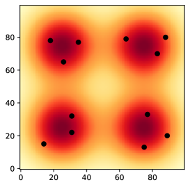
(b) Three stations per city

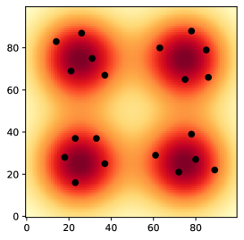
(c) Five stations per city

Figure 4: Location of the charging stations

For our experiments, we derived five sets of instances from the original instances. In the first set of instances, vehicles cannot recharge the battery during the route. In the second set of instances, vehicles can only recharge the battery at the depot. In the other set of instances, vehicles can recharge the battery at the depot and at public charging infrastructure close to one of the four city centres. The number of charging stations available ranges from one per city to five per city and their locations are illustrated in Figure 4.

In order to determine time-dependent travel time and consumption functions for any pair of locations, we determine a time-dependent shortest path for different start times distributed over the planning horizon, assuming that the vehicle can only move one unit left, right, up, or down, and $\sqrt{2}$ units in diagonal direction. A time-dependent travel time function is then determined by fitting a piecewise linear function to the duration of the time-dependent shortest paths. For each of the time-dependent shortest paths, we determine the energy consumed along the path by accumulating the speed-dependent energy consumption (Galvin 2017) for each point traversed along the path. Then, the time-dependent consumption function is obtained by fitting a piecewise linear function to the energy consumption of the time-dependent shortest paths. The details of the instance generator including the source code can be found online at https://github.com/SteffenPottel/td_vrptw_instancegenerator.

The instances are heuristically solved using an adaptation of the savings algorithm (Clarke and Wright 1964), where routes are evaluated using the approaches presented in this paper. Since vehicles and the corresponding driver are the main cost-components in last-mile delivery operations, we optimize over the total number of vehicles first and, as a second criterion, over the total completion time. The latter includes, in particular, the time to return to the depot. In order to allow recharging of the battery at the depot or at public charging stations we allow vehicles to take a detour via a charging station whenever the increase in the travel distance does not exceed $\sqrt{2}$ times the direct distance between delivery locations. If multiple charging stations satisfy this criterion, then the charging station with the smallest detour is chosen. The delivery companies partnering in the project expressed that they want to avoid short and possibly avoidable stops at charging stations. By setting the duration of the replenishment to a constant value we penalize recharging when the energy level of the battery is still high.

We implemented our algorithms in C++ and ran the experiments on a single core of an Intel Core i7-7700HQ CPU with 2.80GHz. For comparison purposes we ran experiments using CPLEX for solving for the mixed integer program provided in Appendix A.

Tables 1 and 2 provide an overview over the results of our experiments. Detailed results of our experiments can be found in Appendix C. The first column in the tables indicates the solver used for route evaluations. The dynamic discretization discovery approach is denoted by DDD, the dynamic discretization discovery approach with preloading of vertices is denoted by DDD-PL, and the approach using the mixed integer programming solver is denoted by MIP. The second column lists the number of charging stations available. The third and fourth column show the average computation time (in seconds) until termination of the savings algorithm, and the computation time (in seconds) per route evaluation. The fifth and six column report the average number of vehicles and the average total completion time. The next two columns indicate the number of routes in which the vehicle recharges the battery at a service station (or the depot) and the total number of replenishments. The last column indicates the number of instances for which the savings algorithm terminated within the run time limit of 7200 seconds.

Solver	Charging	Avg. CPU	CPU per Evaluation	Avg. Veh.	Avg. Compl.	Replenishments	Routes w. Repl.	Terminated
DDD	none	82.4	0.000182	18.0	5949.4	0	0	29
DDD	Depot	93.9	0.000161	18.0	5948.2	6	6	29
DDD	Depot + 1 per city	134.8	0.000203	18.1	5958.3	9	9	29
DDD	Depot + 3 per city	135.3	0.000186	18.0	5954.8	10	10	29
DDD	Depot + 5 per city	146.9	0.000198	18.0	5960.5	10	10	29
DDD-PL	none	72.6	0.000162	18.0	5949.4	0	0	29
DDD-PL	Depot	75.8	0.000128	18.0	5948.2	6	6	29
DDD-PL	Depot + 1 per city	84.0	0.000127	18.1	5958.3	9	9	29
DDD-PL	Depot + 3 per city	81.1	0.000113	18.0	5954.8	10	10	29
DDD-PL	Depot + 5 per city	88.4	0.000121	18.0	5960.5	10	10	29
MIP	none	2508.0	0.005232	18.1	5950.6	0	0	29
MIP	Depot	3299.9	0.005505	18.4	5752.5	4	4	28
MIP	Depot + 1 per city	3621.5	0.005620	18.4	5753.5	7	7	28
MIP	Depot + 3 per city	3345.9	0.005407	19.3	5622.5	5	5	23
MIP	Depot + 5 per city	3282.6	0.005342	19.5	5753.8	6	6	22

Table 1: Results averaged over 29 instances of type C1, R1, and RC1.

Solver	Charging	Avg. CPU	CPU per Evaluation	Avg. Veh.	Avg. Compl.	Replenishments	Routes w. Repl.	Terminated
DDD	none	718.2	0.001021	9.6	8386.9	0	0	27
DDD	Depot	934.5	0.000802	6.7	6936.7	188	124	27
DDD	Depot + 1 per city	1254.9	0.000853	6.8	6884.8	190	122	27
DDD	Depot + 3 per city	2021.6	0.000739	6.2	6430.8	189	113	26
DDD	Depot + 5 per city	2306.4	0.000761	6.3	6858.1	172	105	23
DDD-PL	none	721.2	0.001020	9.6	8386.9	0	0	27
DDD-PL	Depot	640.4	0.000552	6.7	6936.7	188	124	27
DDD-PL	Depot + 1 per city	739.2	0.000513	6.8	6884.8	190	122	27
DDD-PL	Depot + 3 per city	1030.3	0.000351	6.2	6654.4	197	117	27
DDD-PL	Depot + 5 per city	1045.7	0.000305	6.2	6854.9	194	116	26
MIP	none	3729.6	0.005853	10.0	9056.6	0	0	21
MIP	Depot	4877.2	0.005443	7.1	8100.1	55	40	8
MIP	Depot + 1 per city	5542.7	0.005701	6.2	7588.0	29	25	5
MIP	Depot + 3 per city	6725.1	0.005562	4.0	10778.2	1	1	1
MIP	Depot + 5 per city	6230.4	0.005494	4.0	10746.7	3	3	1

Table 2: Results averaged over 27 instances of type C2, R2, and RC2.

As we can see in Tables 1 and 2, the dynamic discretization discovery approaches are magnitudes faster than the savings algorithm using the MIP formulation for route evaluations which fails to terminate for many of the instances within the run time limit of 7200 seconds. We have to note, that although the route evaluations are embedded within the same savings algorithm, the MIP approach can produce results that differ from those of the DDD approaches, because the MIP formulation is not restricted to the discretization. Small deviations in calculating the savings can result in different rankings of the savings and ultimately in different routes being generated.

Instances belonging to sets C1, R1, and RC1, have a smaller freight capacity and a shorter planning horizon compared to instances belonging to sets C2, R2, and RC2. Therefore, more vehicles are used for instances of sets C1, R1, and RC1 than for instances of sets C2, R2, and RC2. Thus routes for instances in sets C1, R1, and RC1 visit fewer customers and the approach requires significantly less computational effort than for instances of sets C2, R2, and RC2.

With fewer stops per route, the likelihood of running out of electric energy is much smaller. In fact, the solutions for instances of sets R1 and RC1 have no recharging stops at all, because these instances have a very short planning horizon, leaving little time to sensibly recharge batteries. For instances in sets C2, R2, and RC2, the freight capacity and planning horizons are larger. Therefore, less vehicles are used and many more routes make use of the possibility to recharge the batteries.

With an increasing number of charging stations, the number of alternative routes via charging stations increases and so does the computational effort required for evaluating these alternatives. We can see that preloading of vertices helps stabilizing the runtime of the algorithm and leads to significantly shorter computation times for instances with many charging possibilities. With preloading of vertices, the dynamic discretization discovery approach is able to (heuristically) solve almost all of the instances except for instance r211 with five charging stations per city within the run time limit. Without run time limit, instance r211 with five charging stations per city can be solved in 8027.5 seconds.

An interesting observation from an application point of view is that the possibility to recharge the battery during a route can significantly reduce the number of vehicles required as well as the total completion time. Table 2 indicates that for instances in sets C2, R2, and RC2, the number of routes required can be reduced by approximately one third if vehicles can recharge batteries while they are on route. This demonstrates the importance of considering replenishments within scheduling. Furthermore, it can be seen that the number of vehicles required is not significantly reduced with an increasing number of charging stations. In fact, the possibility to recharge the battery at the depot already accounts for the main benefit in terms of the number of vehicles required. Additional public charging infrastructure may furthermore reduce the detour required to reach a charging station and thus can contribute to smaller total completion times and less routes requiring replenishments.

7 Conclusions

In this paper we introduce a time-dependent activity scheduling problem in which activities consume a limited resource during execution and activity durations and resource consumptions are time-dependent. Moreover, we study the case in which the resource can be replenished between conducting subsequent activities. We propose a dynamic discretization discovery algorithm which is based on partially time-expanded networks which are dynamically filled with additional vertices. The dynamic discretization discovery algorithm can be used for general duration and consumption functions and only requires the first-in-first-out property for activity durations. For the case that the dynamic discretization discovery is embedded in an iterative solution procedure that frequently evaluates activity sequences that start with the same activities, we propose to preload the partially expanded network with vertices generated in previous iterations. This preloading of vertices can significantly reduce the computational effort required.

We evaluate our approaches on a case of determining routes for a fleet of electric delivery vehicles for last-mile deliveries. Our experimental results indicate that the dynamic discretization discovery algorithm is magnitudes faster than the commercial solver CPLEX using a mixed integer programming formulation of the problem. Furthermore, our experiments show that for our instances, which are motivated by the real-life case of last-mile delivery operations, the possibility to recharge batteries en-route can significantly reduce the number of vehicles required and the total completion time.

Appendix

Appendix A Mixed-integer program for piecewise linear duration and consumption functions

In this appendix we provide a formulation of the TDASPR under the assumption that functions $\tau_{i}(t)$, $\theta_{i}(t)$, and $\rho_{i}(t)$ are non-negative, piecewise linear, and lower semi-continuous for each $1\leq i\leq n$ and that the replenishment duration $\Delta_{i}$ is a constant for each $1\leq i\leq n$. Like before we assume that the FIFO property holds, i.e., that $\theta_{i}(t)$ is non-decreasing. Note that we do not require $\tau_{i}(t)$, $\theta_{i}(t)$, and $\rho_{i}(t)$ to be continuous. This allows us to consider applications such as durations of trips conducted with public transport services where discontinuities occur when the scheduled departure time is missed and waiting time until the next scheduled departure needs to be considered.

Let $S^{\tau}_{i}$ and $S^{\rho}_{i}$ denote the set of piecewise linear segments of $\tau_{i}$ and $\rho_{i}$. For each linear segment $s\in S^{\tau}_{i}\cup S^{\rho}_{i}$, let $e_{s}$ and $l_{s}$ denote the start and end of the segment and let $a_{s}$ denote the slope and $b_{s}$ the intercept of the respective linear function. Thus, if the start time $t_{i}$ of activity $i$ is within segment $s\in S^{\tau}_{i}$, then $\tau_{i}(t_{i})=a_{s}t_{i}+b_{s}$.

With this, the problem can be modelled with binary variables $x_{i,s}$ indicating whether segment $s\in S^{\tau}_{i}$ of the duration function or segment $s\in S^{\rho}_{i}$ of the consumption function is used for activity $i$. A binary variable $y_{i}$ indicates whether the resource is replenished after conducting the activity $i$, linear variables $d_{i}$ and $q_{i}$ indicate the duration and resource consumption of activity $i$, and $t_{i}$ indicates the start time of activity $i$. Linear variables $t_{i,s}$ indicate time values for activity $i$ associated to segment $s\in S^{\tau}_{i}$ of the duration function or for segment $s\in S^{\rho}_{i}$ of the consumption function.

The TDASP with piecewise linear duration and consumption functions can be formulated as a mixed-integer program by

minimise

$$t_{n}+d_{n}$$ (11)

subject to

$$\sum_{s\in S^{\tau}_{i}}x_{i,s}=1\textrm{ for all }1\leq i\leq n$$ (12a)

$$e_{s}x_{i,s}\leq t_{i,s}\leq l_{s}x_{i,s}\textrm{ for all }1\leq i\leq n,s\in S^{\tau}_{i}$$ (12b)

$$t_{i}=\sum_{s\in S^{\tau}_{i}}t_{i,s}\textrm{ for all }1\leq i\leq n$$ (12c)

$$d_{i}=\sum_{s\in S^{\tau}_{i}}(a_{s}t_{i,s}+b_{s}x_{i,s})\textrm{ for all }1\leq i\leq n$$ (12d)

$$t_{i}+d_{i}+\Delta_{i}y_{i}\leq t_{i+1}\textrm{ for all }1\leq i<n$$ (12e)

$$\sum_{s\in S^{\rho}_{i}}x_{i,s}=1\textrm{ for all }1\leq i\leq n$$ (13a)

$$e_{s}x_{i,s}\leq t_{i,s}\leq l_{s}x_{i,s}\textrm{ for all }1\leq i\leq n,s\in S^{\rho}_{i}$$ (13b)

$$t_{i}=\sum_{s\in S^{\rho}_{i}}t_{i,s}\textrm{ for all }1\leq i\leq n$$ (13c)

$$q_{i}=\sum_{s\in S^{\rho}_{i}}(a_{s}t_{i,s}+b_{s}x_{i,s})\textrm{ for all }1\leq i\leq n$$ (13d)

$$\sum_{k=i}^{j}q_{k}\leq Q+M\sum_{k=i}^{j-1}y_{k}\textrm{ for all }1\leq i\leq j\leq n$$ (13e)

$$x_{i,s}\in\{0,1\}\textrm{ for all }s\in S^{\tau}_{i}\cup S^{\rho}_{i},1\leq i\leq n$$ (14)

$$y_{i}\in\{0,1\}\textrm{ for all }1\leq i\leq n$$ (15)

The objective (11) is to minimise the completion time. Constraint (12a) ensures that for each activity exactly one of the time segments is selected. Constraints (12b) and (12c) ensure that $t_{i,s}$ is zero if $x_{i,s}=0$ and $t_{i,s}\in[e_{s},l_{s}]$ if $x_{i,s}=1$, and that the start time of activity $i$ is set accordingly. Note that the boundary values of $[e_{s},l_{s}]$ might not belong to the segment $s$ because we do not require continuity of the functions. Due to the lower semi-continuity, however, this is not a problem in an optimal solution. The duration $d_{i}$ of activity $i$ can be obtained by constraint (12d). Because of constraint (12e), the start time of any activity must not be before the completion time of the previous activity plus the time required for a potential replenishment. Constraints (13a) to (13d) are analogous to constraints (12a) to (12d) for the resource consumption. Constraint (13e) requires that the cumulative resource consumption of any sequence of activities does not exceed $Q$ unless the resource is replenished. Lastly, the domain of the binary variables is given by (14) and (15).

Appendix B Restrictions on replenishments

A variation of the TDASPR, in which replenishments are forbidden or required after certain activities, can be obtained by constraining the binary variables indicating the choice of whether to conduct a replenishment or not. This can be achieved by adding a constraint $y_{i}=0$ or $y_{i}=1$ for each activity $i$ which prohibits or requires a replenishment after its completion in the problems given by (5) to (9) or (11) to (15).

If a replenishment is not allowed after an activity, we can avoid replenishments by adapting Algorithm 4 in such a way that the earliest time after the replenishment $t^{*}$ is set to a value that exceeds $l_{i+1}$ in line 4.

Let us now consider the case that a replenishment is required after activity $i$. In this case Property 2 loses its relevance for all vertices of activity $i$, because the property does not consider the duration of the required replenishment. The main purpose of Property 2 was to ensure that the vertex representing the earliest possible time at which the next activity can be conducted is included in the partially expanded network. In Algorithm 4, this is achieved by line 4 which includes a vertex for the next activity and the earliest time after the required replenishment. We can adapt Algorithm 4 in such a way that lines 4 to 4, which update the labels assuming that no replenishment is conducted, are skipped if a replenishment is required. Furthermore, the condition in line 2 of function ${\tt DDD\!::\!addRecursive}$ can be changed in such a way that the recursive insertion of vertices is terminated if a replenishment is required after the current activity. With these changes our approach can be used to solve the TDASPR with required replenishments even if Property 2 does not hold for activities requiring a replenishment.

Appendix C Detailed results

Tables 3 to  7 show detailed results of our computational experiments. The first column gives the name of the instance. The results for the approach based on dynamic discretization discovery with replenishments (DDD) are given in columns 2 to 5. The results for the dynamic discretization discover approach with replenishments and preloading (DDD-PL) are given in columns 6 to 9. The results for the approach using CPLEX for solving for the mixed integer program (MIP) are given in columns 10 to 13. For each approach, the total computation time is given in the column titled CPU, the number of vehicles required is given in the column titled Veh., the total completion time is given in the column titled Compl., and the number of replenishments at service stations is given in the column titled Repl.. Dashes in the columns for MIP indicate that no solution was found within the time limit of 7200 seconds. For the dynamic discretization discovery approaches DDD and DDD-PL, the results violating the time limit are written in italic.

	DDD				DDD-PL				MIP
Instance	CPU	Veh.	Compl.	Repl.	CPU	Veh.	Compl.	Repl.	CPU	Veh.	Compl.	Repl.
c101	101.4	13	11589.1	0	97.8	13	11589.1	0	1083.0	14	11507.9	0
c102	645.3	16	12064.9	0	628.2	16	12064.9	0	2189.1	15	11974.3	0
c103	271.2	11	11809.4	0	256.5	11	11809.4	0	3308.8	12	11978.7	0
c104	60.2	11	11788.7	0	49.2	11	11788.7	0	4389.2	11	11644.2	0
c105	96.4	15	10946.8	0	89.1	15	10946.8	0	1505.1	14	10930.6	0
c106	116.9	16	12357.3	0	110.3	16	12357.3	0	1601.9	16	12432.2	0
c107	126.7	13	10653.1	0	115.6	13	10653.1	0	2054.6	12	10487.1	0
c108	139.0	13	10884.0	0	122.6	13	10884.0	0	2351.3	15	11077.0	0
c109	160.4	13	10612.8	0	143.1	13	10612.8	0	3379.3	13	10606.5	0
c201	29.4	5	11321.1	0	7.3	5	11321.1	0	2054.1	5	11317.0	0
c202	417.9	8	17256.2	0	382.6	8	17256.2	0	2863.3	9	17647.4	0
c203	143.3	9	17404.2	0	120.2	9	17404.2	0	4360.3	11	18616.1	0
c204	4599.1	8	16319.8	0	4804.2	8	16319.8	0	—	—	—	—
c205	47.6	5	11123.6	0	16.2	5	11123.6	0	2662.4	5	11119.2	0
c206	171.2	8	15428.4	0	126.0	8	15428.4	0	2902.9	8	15554.2	0
c207	248.5	10	19200.6	0	202.9	10	19200.6	0	2825.2	10	18998.1	0
c208	97.1	5	10839.4	0	42.9	5	10839.4	0	5048.7	5	10834.5	0
r101	21.2	28	4596.6	0	18.5	28	4596.6	0	473.6	28	4619.5	0
r102	37.3	23	3864.5	0	31.3	23	3864.5	0	1767.6	23	3835.1	0
r103	33.7	19	3470.5	0	24.4	19	3470.5	0	2853.6	19	3491.1	0
r104	25.4	15	2951.3	0	12.0	15	2951.3	0	4224.7	14	2839.2	0
r105	44.9	22	3717.0	0	41.4	22	3717.0	0	852.4	23	3913.1	0
r106	38.0	21	3373.2	0	29.4	21	3373.2	0	2228.1	21	3332.1	0
r107	36.0	19	3093.4	0	25.7	19	3093.4	0	3216.4	20	3241.5	0
r108	24.6	16	2937.1	0	9.9	16	2937.1	0	4398.2	16	2917.9	0
r109	56.4	20	3273.5	0	48.4	20	3273.5	0	1811.9	19	3185.3	0
r110	37.7	18	2964.8	0	26.9	18	2964.8	0	2859.1	18	3036.1	0
r111	33.4	18	3126.4	0	21.3	18	3126.4	0	3153.0	18	3079.2	0
r112	28.2	15	2638.0	0	9.2	15	2638.0	0	4878.3	15	2632.5	0
r201	254.3	12	6799.5	0	246.2	12	6799.5	0	2502.3	12	6839.2	0
r202	604.6	11	6422.3	0	592.1	11	6422.3	0	3366.1	11	6204.6	0
r203	415.7	9	4988.8	0	420.5	9	4988.8	0	4085.9	9	4880.5	0
r204	783.1	8	4210.2	0	797.1	8	4210.2	0	—	—	—	—
r205	493.0	10	5732.0	0	491.3	10	5732.0	0	3678.4	11	6038.5	0
r206	1064.1	10	5211.6	0	1155.0	10	5211.6	0	4797.2	10	5341.0	0
r207	814.1	9	4700.4	0	844.3	9	4700.4	0	5726.8	9	4453.6	0
r208	810.9	8	3528.3	0	820.8	8	3528.3	0	—	—	—	—
r209	785.4	11	5820.9	0	784.0	11	5820.9	0	4621.4	11	5785.2	0
r210	536.3	10	5400.0	0	543.4	10	5400.0	0	4554.3	11	5888.0	0
r211	1463.2	9	4499.5	0	1501.0	9	4499.5	0	—	—	—	—
rc101	26.5	25	4553.7	0	24.5	25	4553.7	0	668.5	24	4400.1	0
rc102	34.5	23	4007.6	0	28.9	23	4007.6	0	1702.7	23	3933.6	0
rc103	31.0	21	3739.8	0	22.4	21	3739.8	0	2748.0	21	3774.4	0
rc104	30.2	15	3123.7	0	16.0	15	3123.7	0	4073.1	16	3198.8	0
rc105	36.9	22	4030.0	0	32.8	22	4030.0	0	1348.8	24	4142.6	0
rc106	47.9	22	3735.4	0	42.8	22	3735.4	0	1360.1	21	3661.8	0
rc107	24.8	22	3515.4	0	16.2	22	3515.4	0	2488.5	22	3504.7	0
rc108	23.7	17	3115.6	0	10.1	17	3115.6	0	3763.3	18	3191.4	0
rc201	479.4	14	7851.4	0	470.6	14	7851.4	0	2118.6	14	7992.2	0
rc202	346.8	13	7266.6	0	345.7	13	7266.6	0	3475.4	12	7203.4	0
rc203	417.6	11	5670.8	0	400.1	11	5670.8	0	4632.7	11	5723.4	0
rc204	941.1	9	4235.3	0	906.5	9	4235.3	0	—	—	—	—
rc205	495.4	13	7177.7	0	489.4	13	7177.7	0	3102.3	13	7081.8	0
rc206	772.5	12	6883.9	0	768.8	12	6883.9	0	4046.7	12	6880.8	0
rc207	761.0	12	6388.6	0	755.6	12	6388.6	0	4897.0	12	5790.4	0
rc208	1399.6	11	4764.5	0	1438.3	11	4764.5	0	—	—	—	—

Table 3: Results for instances without service stations.

	DDD				DDD-PL				MIP
Instance	CPU	Veh.	Compl.	Repl.	CPU	Veh.	Compl.	Repl.	CPU	Veh.	Compl.	Repl.
c101	112.7	13	11589.1	0	105.7	13	11589.1	0	1570.7	14	11507.9	0
c102	662.5	17	12063.2	1	650.8	17	12063.2	1	3620.6	15	11974.3	0
c103	296.2	11	12038.8	2	274.7	11	12038.8	2	5572.4	12	12213.4	2
c104	80.9	11	11590.4	1	56.8	11	11590.4	1	—	—	—	—
c105	105.9	15	10946.8	0	92.0	15	10946.8	0	2194.6	14	10930.6	0
c106	124.4	16	12292.3	2	114.3	16	12292.3	2	2367.1	16	12343.1	2
c107	138.6	13	10653.1	0	120.5	13	10653.1	0	2999.0	12	10487.1	0
c108	151.1	13	10884.0	0	127.1	13	10884.0	0	3583.9	15	11077.0	0
c109	179.7	13	10612.8	0	147.9	13	10612.8	0	5342.9	13	10606.5	0
c201	78.1	4	10800.4	2	16.1	4	10800.4	2	3493.4	4	10864.3	2
c202	166.5	8	13213.7	11	33.7	8	13213.7	11	5350.8	9	14985.1	9
c203	947.5	6	14026.1	8	700.4	6	14026.1	8	—	—	—	—
c204	829.3	5	13141.1	8	671.6	5	13141.1	8	—	—	—	—
c205	119.8	4	10609.8	2	36.4	4	10609.8	2	4953.0	4	10576.7	2
c206	481.9	5	12078.3	8	125.9	5	12078.3	8	—	—	—	—
c207	742.5	5	13219.8	11	465.2	5	13219.8	11	—	—	—	—
c208	278.8	4	10388.0	2	140.0	4	10388.0	2	—	—	—	—
r101	21.4	28	4596.6	0	18.9	28	4596.6	0	486.3	28	4619.5	0
r102	41.0	23	3864.5	0	32.5	23	3864.5	0	2332.4	23	3835.1	0
r103	44.3	19	3470.5	0	26.4	19	3470.5	0	4156.0	19	3491.1	0
r104	42.7	15	2951.3	0	14.5	15	2951.3	0	6477.7	14	2839.2	0
r105	46.0	22	3717.0	0	41.5	22	3717.0	0	884.5	23	3913.1	0
r106	42.9	21	3373.2	0	30.2	21	3373.2	0	2896.1	21	3332.1	0
r107	46.4	19	3093.4	0	27.5	19	3093.4	0	4605.1	20	3241.5	0
r108	42.1	16	2937.1	0	12.4	16	2937.1	0	6614.1	16	2917.9	0
r109	57.3	20	3273.5	0	48.9	20	3273.5	0	1912.1	19	3185.3	0
r110	40.5	18	2964.8	0	27.5	18	2964.8	0	3259.8	18	3036.1	0
r111	38.8	18	3126.4	0	22.7	18	3126.4	0	3862.2	18	3079.2	0
r112	33.3	15	2638.0	0	10.5	15	2638.0	0	5568.3	15	2632.5	0
r201	244.7	7	5173.2	10	226.5	7	5173.2	10	3869.1	7	5197.1	8
r202	1636.8	9	5846.2	8	1294.1	9	5846.2	8	6243.5	8	5509.5	7
r203	587.8	8	4510.7	5	408.5	8	4510.7	5	—	—	—	—
r204	307.2	5	3675.6	6	173.5	5	3675.6	6	—	—	—	—
r205	1229.0	8	4897.6	7	795.3	8	4897.6	7	—	—	—	—
r206	1649.9	7	4529.1	7	1147.0	7	4529.1	7	—	—	—	—
r207	758.8	7	3606.0	4	467.2	7	3606.0	4	—	—	—	—
r208	919.6	5	3417.8	6	474.3	5	3417.8	6	—	—	—	—
r209	1403.9	7	4583.4	8	935.3	7	4583.4	8	—	—	—	—
r210	2123.2	7	4276.1	6	1503.8	7	4276.1	6	—	—	—	—
r211	2597.0	6	3616.2	5	1894.3	6	3616.2	5	—	—	—	—
rc101	35.5	25	4553.7	0	24.0	25	4553.7	0	694.4	24	4400.1	0
rc102	48.3	23	4007.6	0	28.9	23	4007.6	0	2059.9	23	3933.6	0
rc103	50.0	21	3739.8	0	22.8	21	3739.8	0	3635.7	21	3774.4	0
rc104	56.5	15	3123.7	0	17.5	15	3123.7	0	5767.0	16	3198.8	0
rc105	49.4	22	4030.0	0	32.5	22	4030.0	0	1452.3	24	4142.6	0
rc106	64.1	22	3735.4	0	42.1	22	3735.4	0	1437.7	21	3661.8	0
rc107	35.7	22	3515.4	0	16.3	22	3515.4	0	2801.4	22	3504.7	0
rc108	35.6	17	3115.6	0	10.4	17	3115.6	0	4243.9	18	3191.4	0
rc201	1068.9	11	6859.0	7	760.0	11	6859.0	7	3792.7	8	6058.0	8
rc202	614.7	8	5630.5	9	435.3	8	5630.5	9	5983.0	8	5627.6	9
rc203	484.1	9	4591.2	7	312.3	9	4591.2	7	—	—	—	—
rc204	1307.1	5	3924.7	6	940.8	5	3924.7	6	—	—	—	—
rc205	919.5	10	6271.4	10	667.1	10	6271.4	10	5332.3	9	5982.3	10
rc206	1288.5	7	5019.8	9	893.5	7	5019.8	9	—	—	—	—
rc207	831.2	9	5249.0	9	575.2	9	5249.0	9	—	—	—	—
rc208	1614.4	6	4136.9	7	1196.6	6	4136.9	7	—	—	—	—

Table 4: Results for instances with recharging at the depot.

	DDD				DDD-PL				MIP
Instance	CPU	Veh.	Compl.	Repl.	CPU	Veh.	Compl.	Repl.	CPU	Veh.	Compl.	Repl.
c101	216.7	13	11589.1	0	148.3	13	11589.1	0	1839.8	14	11507.9	0
c102	898.6	17	12063.2	1	663.6	17	12063.2	1	4255.9	15	12042.2	2
c103	629.0	13	12129.1	4	416.1	13	12129.1	4	6915.7	12	12219.9	2
c104	122.2	11	11719.3	2	60.2	11	11719.3	2	—	—	—	—
c105	144.1	15	10946.8	0	94.9	15	10946.8	0	2538.3	14	10930.6	0
c106	185.9	16	12365.6	2	126.3	16	12365.6	2	3064.5	16	12297.4	3
c107	189.1	13	10653.1	0	123.8	13	10653.1	0	3476.7	12	10487.1	0
c108	214.9	13	10884.0	0	134.2	13	10884.0	0	4384.8	15	11077.0	0
c109	249.4	13	10612.8	0	155.8	13	10612.8	0	6372.4	13	10606.5	0
c201	149.3	4	10754.0	2	19.7	4	10754.0	2	4363.4	4	10880.6	2
c202	799.7	8	13114.4	10	211.8	8	13114.4	10	—	—	—	—
c203	2078.1	6	14079.3	7	1006.9	6	14079.3	7	—	—	—	—
c204	3071.9	5	13153.1	8	1559.3	5	13153.1	8	—	—	—	—
c205	232.9	4	10622.9	2	38.4	4	10622.9	2	6382.4	4	10656.9	2
c206	932.9	5	12398.6	9	335.1	5	12398.6	9	—	—	—	—
c207	1361.8	6	13238.2	10	331.9	6	13238.2	10	—	—	—	—
c208	496.5	4	10388.0	2	161.3	4	10388.0	2	—	—	—	—
r101	28.2	28	4596.6	0	18.9	28	4596.6	0	488.0	28	4619.5	0
r102	54.7	23	3864.5	0	32.6	23	3864.5	0	2384.4	23	3835.1	0
r103	59.2	19	3470.5	0	26.4	19	3470.5	0	4282.0	19	3491.1	0
r104	57.7	15	2951.3	0	14.9	15	2951.3	0	6679.9	14	2839.2	0
r105	60.1	22	3717.0	0	42.1	22	3717.0	0	880.3	23	3913.1	0
r106	56.9	21	3373.2	0	30.8	21	3373.2	0	2952.0	21	3332.1	0
r107	62.6	19	3093.4	0	27.8	19	3093.4	0	4969.0	20	3241.5	0
r108	56.8	16	2937.1	0	12.9	16	2937.1	0	6827.5	16	2917.9	0
r109	75.5	20	3273.5	0	48.7	20	3273.5	0	1916.4	19	3185.3	0
r110	54.1	18	2964.8	0	27.5	18	2964.8	0	3299.7	18	3036.1	0
r111	51.6	18	3126.4	0	22.8	18	3126.4	0	3975.8	18	3079.2	0
r112	44.8	15	2638.0	0	10.5	15	2638.0	0	5667.4	15	2632.5	0
r201	362.1	8	5228.0	8	253.5	8	5228.0	8	4074.7	7	5237.2	9
r202	1705.6	8	5562.3	7	1269.4	8	5562.3	7	6423.5	8	5408.0	7
r203	561.2	8	4493.1	5	390.5	8	4493.1	5	—	—	—	—
r204	849.3	5	3735.3	6	510.2	5	3735.3	6	—	—	—	—
r205	1721.7	7	4660.5	7	1159.9	7	4660.5	7	—	—	—	—
r206	2038.9	7	4570.1	7	1455.0	7	4570.1	7	—	—	—	—
r207	669.9	7	3586.8	4	373.7	7	3586.8	4	—	—	—	—
r208	996.6	5	3303.6	5	539.1	5	3303.6	5	—	—	—	—
r209	1829.5	8	4613.9	7	1216.3	8	4613.9	7	—	—	—	—
r210	913.2	8	4598.5	7	621.5	8	4598.5	7	—	—	—	—
r211	2836.2	6	3612.4	5	2059.4	6	3612.4	5	—	—	—	—
rc101	35.7	25	4553.7	0	24.1	25	4553.7	0	707.4	24	4400.1	0
rc102	50.4	23	4007.6	0	29.2	23	4007.6	0	2307.7	23	3933.6	0
rc103	54.1	21	3739.8	0	23.5	21	3739.8	0	4111.0	21	3774.4	0
rc104	64.3	15	3123.7	0	18.4	15	3123.7	0	6503.2	16	3198.8	0
rc105	50.5	22	4030.0	0	32.8	22	4030.0	0	1548.1	24	4142.6	0
rc106	65.3	22	3735.4	0	42.1	22	3735.4	0	1513.0	21	3661.8	0
rc107	37.1	22	3515.4	0	16.5	22	3515.4	0	2953.0	22	3504.7	0
rc108	39.1	17	3115.6	0	11.0	17	3115.6	0	4588.9	18	3191.4	0
rc201	500.4	9	6035.4	10	313.2	9	6035.4	10	6469.3	8	5757.2	9
rc202	506.7	9	5530.7	11	342.1	9	5530.7	11	—	—	—	—
rc203	484.8	8	4406.0	8	317.1	8	4406.0	8	—	—	—	—
rc204	501.9	6	4009.1	6	287.5	6	4009.1	6	—	—	—	—
rc205	1207.3	9	5812.7	12	818.9	9	5812.7	12	—	—	—	—
rc206	2284.8	8	5272.5	9	1426.5	8	5272.5	9	—	—	—	—
rc207	1412.4	8	5032.1	10	902.4	8	5032.1	10	—	—	—	—
rc208	3377.5	7	4078.1	6	2038.5	7	4078.1	6	—	—	—	—

Table 5: Results for instances with recharging at the depot and one station per city.

	DDD				DDD-PL				MIP
Instance	CPU	Veh.	Compl.	Repl.	CPU	Veh.	Compl.	Repl.	CPU	Veh.	Compl.	Repl.
c101	169.5	13	11589.1	0	115.3	13	11589.1	0	2059.8	14	11507.9	0
c102	930.9	17	12063.2	1	681.4	17	12063.2	1	4734.5	15	12079.1	1
c103	432.2	11	11992.5	3	292.6	11	11992.5	3	—	—	—	—
c104	152.9	11	11732.0	3	63.6	11	11732.0	3	—	—	—	—
c105	156.8	15	10946.8	0	99.1	15	10946.8	0	2851.8	14	10930.6	0
c106	202.5	16	12389.2	3	130.6	16	12389.2	3	3611.1	16	12262.3	4
c107	202.1	13	10653.1	0	128.3	13	10653.1	0	3928.6	12	10487.1	0
c108	246.3	13	10884.0	0	149.1	13	10884.0	0	5407.3	15	11077.0	0
c109	272.4	13	10612.8	0	161.3	13	10612.8	0	—	—	—	—
c201	414.4	4	10758.8	2	31.1	4	10758.8	2	6725.1	4	10778.2	1
c202	1162.7	7	12369.5	9	206.6	7	12369.5	9	—	—	—	—
c203	2520.5	6	14003.2	8	579.7	6	14003.2	8	—	—	—	—
c204	4710.0	5	13259.3	7	1262.7	5	13259.3	7	—	—	—	—
c205	677.5	4	10071.8	2	63.4	4	10071.8	2	—	—	—	—
c206	1413.5	5	12160.6	8	171.0	5	12160.6	8	—	—	—	—
c207	12235.4	5	12469.8	8	6787.1	5	12469.8	8	—	—	—	—
c208	2069.5	4	10040.9	2	612.1	4	10040.9	2	—	—	—	—
r101	28.5	28	4596.6	0	18.9	28	4596.6	0	504.2	28	4619.5	0
r102	58.1	23	3864.5	0	33.3	23	3864.5	0	2754.6	23	3835.1	0
r103	67.7	19	3470.5	0	27.8	19	3470.5	0	5128.7	19	3491.1	0
r104	68.4	15	2951.3	0	16.4	15	2951.3	0	—	—	—	—
r105	60.8	22	3717.0	0	41.8	22	3717.0	0	931.2	23	3913.1	0
r106	61.2	21	3373.2	0	31.5	21	3373.2	0	3440.5	21	3332.1	0
r107	71.3	19	3093.4	0	28.8	19	3093.4	0	5651.0	20	3241.5	0
r108	68.0	16	2937.1	0	14.2	16	2937.1	0	—	—	—	—
r109	79.1	20	3273.5	0	50.2	20	3273.5	0	2070.6	19	3185.3	0
r110	58.9	18	2964.8	0	28.5	18	2964.8	0	3690.6	18	3036.1	0
r111	59.8	18	3126.4	0	23.4	18	3126.4	0	4616.6	18	3079.2	0
r112	56.5	15	2638.0	0	11.8	15	2638.0	0	6645.8	15	2632.5	0
r201	716.5	7	5192.1	9	352.9	7	5192.1	9	—	—	—	—
r202	1038.9	8	5185.6	10	688.2	8	5185.6	10	—	—	—	—
r203	903.3	8	4053.7	7	535.2	8	4053.7	7	—	—	—	—
r204	324.3	4	3698.4	5	143.1	4	3698.4	5	—	—	—	—
r205	4064.5	7	4353.7	8	1197.2	7	4353.7	8	—	—	—	—
r206	2180.7	6	4183.6	8	1021.8	6	4183.6	8	—	—	—	—
r207	6237.2	6	3756.8	5	983.5	6	3756.8	5	—	—	—	—
r208	1360.3	5	3478.2	6	570.5	5	3478.2	6	—	—	—	—
r209	2220.9	7	4082.1	7	1357.0	7	4082.1	7	—	—	—	—
r210	1814.5	7	4512.7	7	1036.7	7	4512.7	7	—	—	—	—
r211	6747.9	5	3571.9	6	3528.3	5	3571.9	6	—	—	—	—
rc101	36.0	25	4553.7	0	25.0	25	4553.7	0	727.9	24	4400.1	0
rc102	52.1	23	4007.6	0	29.5	23	4007.6	0	2439.6	23	3933.6	0
rc103	58.6	21	3739.8	0	24.7	21	3739.8	0	4504.1	21	3774.4	0
rc104	71.9	15	3123.7	0	19.6	15	3123.7	0	—	—	—	—
rc105	51.6	22	4030.0	0	33.7	22	4030.0	0	1613.9	24	4142.6	0
rc106	65.4	22	3735.4	0	43.3	22	3735.4	0	1538.2	21	3661.8	0
rc107	39.9	22	3515.4	0	17.1	22	3515.4	0	3154.1	22	3504.7	0
rc108	43.6	17	3115.6	0	11.7	17	3115.6	0	4950.6	18	3191.4	0
rc201	559.2	8	5729.6	12	310.7	8	5729.6	12	—	—	—	—
rc202	633.2	8	5248.6	10	415.8	8	5248.6	10	—	—	—	—
rc203	645.4	8	4484.0	7	409.1	8	4484.0	7	—	—	—	—
rc204	634.5	5	3835.8	6	350.5	5	3835.8	6	—	—	—	—
rc205	1166.8	8	5418.7	12	762.6	8	5418.7	12	—	—	—	—
rc206	2217.4	7	4900.0	9	1035.5	7	4900.0	9	—	—	—	—
rc207	1763.2	7	4601.0	9	969.5	7	4601.0	9	—	—	—	—
rc208	4365.7	6	4249.1	8	2435.1	6	4249.1	8	—	—	—	—

Table 6: Results for instances with recharging at the depot and three stations per city.

	DDD				DDD-PL				MIP
Instance	CPU	Veh.	Compl.	Repl.	CPU	Veh.	Compl.	Repl.	CPU	Veh.	Compl.	Repl.
c101	163.7	13	11589.1	0	109.4	13	11589.1	0	2075.3	14	11507.9	0
c102	1131.3	17	12092.0	1	819.4	17	12092.0	1	4747.5	15	12042.2	2
c103	474.6	11	11996.9	3	319.4	11	11996.9	3	—	—	—	—
c104	157.1	11	11734.8	3	65.6	11	11734.8	3	—	—	—	—
c105	157.6	15	10946.8	0	102.0	15	10946.8	0	2830.1	14	10930.6	0
c106	203.1	16	12518.0	3	136.7	16	12518.0	3	3492.2	16	12198.2	4
c107	204.3	13	10653.1	0	131.1	13	10653.1	0	3925.5	12	10487.1	0
c108	280.3	13	10884.0	0	172.2	13	10884.0	0	5678.6	15	11077.0	0
c109	277.5	13	10612.8	0	167.8	13	10612.8	0	—	—	—	—
c201	575.9	4	10778.6	3	42.8	4	10778.6	3	6230.4	4	10746.7	3
c202	1288.0	7	13123.4	9	178.5	7	13123.4	9	—	—	—	—
c203	4930.8	6	14079.3	9	1421.5	6	14079.3	9	—	—	—	—
c204	2570.6	6	14850.6	7	1425.2	6	14850.6	7	—	—	—	—
c205	774.3	4	10224.1	3	77.2	4	10224.1	3	—	—	—	—
c206	3835.5	5	12270.4	8	1221.1	5	12270.4	8	—	—	—	—
c207	8697.8	5	12641.5	10	1124.0	5	12641.5	10	—	—	—	—
c208	1783.7	4	10091.8	2	347.6	4	10091.8	2	—	—	—	—
r101	28.8	28	4596.6	0	18.7	28	4596.6	0	513.5	28	4619.5	0
r102	59.6	23	3864.5	0	33.7	23	3864.5	0	2821.4	23	3835.1	0
r103	68.9	19	3470.5	0	28.3	19	3470.5	0	5237.5	19	3491.1	0
r104	71.6	15	2951.3	0	16.3	15	2951.3	0	—	—	—	—
r105	61.3	22	3717.0	0	41.9	22	3717.0	0	956.4	23	3913.1	0
r106	62.9	21	3373.2	0	32.0	21	3373.2	0	3517.4	21	3332.1	0
r107	73.4	19	3093.4	0	29.0	19	3093.4	0	5790.4	20	3241.5	0
r108	71.6	16	2937.1	0	14.4	16	2937.1	0	—	—	—	—
r109	87.4	20	3273.5	0	56.3	20	3273.5	0	2191.8	19	3185.3	0
r110	62.3	18	2964.8	0	29.4	18	2964.8	0	3970.4	18	3036.1	0
r111	61.8	18	3126.4	0	24.3	18	3126.4	0	4841.8	18	3079.2	0
r112	68.7	15	2638.0	0	12.9	15	2638.0	0	—	—	—	—
r201	439.5	7	5183.7	10	188.9	7	5183.7	10	—	—	—	—
r202	1228.2	7	5076.0	9	827.9	7	5076.0	9	—	—	—	—
r203	655.5	8	4053.2	8	415.9	8	4053.2	8	—	—	—	—
r204	435.3	5	3602.7	5	223.5	5	3602.7	5	—	—	—	—
r205	5509.8	6	4306.3	8	1222.2	6	4306.3	8	—	—	—	—
r206	7646.0	7	4328.1	7	2577.0	7	4328.1	7	—	—	—	—
r207	14042.4	6	3522.8	5	2011.1	6	3522.8	5	—	—	—	—
r208	1836.2	5	3418.4	6	518.6	5	3418.4	6	—	—	—	—
r209	2253.6	6	4304.3	8	1080.7	6	4304.3	8	—	—	—	—
r210	6243.7	7	4274.3	7	2822.7	7	4274.3	7	—	—	—	—
r211	28924.2	5	3508.6	5	8027.5	5	3508.6	5	—	—	—	—
rc101	36.2	25	4553.7	0	24.5	25	4553.7	0	738.7	24	4400.1	0
rc102	53.1	23	4007.6	0	29.7	23	4007.6	0	2517.9	23	3933.6	0
rc103	60.3	21	3739.8	0	24.2	21	3739.8	0	4609.4	21	3774.4	0
rc104	75.4	15	3123.7	0	19.5	15	3123.7	0	—	—	—	—
rc105	52.1	22	4030.0	0	32.9	22	4030.0	0	1677.6	24	4142.6	0
rc106	67.3	22	3735.4	0	43.2	22	3735.4	0	1632.7	21	3661.8	0
rc107	41.0	22	3515.4	0	17.0	22	3515.4	0	3246.2	22	3504.7	0
rc108	47.3	17	3115.6	0	11.8	17	3115.6	0	5205.7	18	3191.4	0
rc201	817.4	8	5783.4	10	422.7	8	5783.4	10	—	—	—	—
rc202	816.7	7	5042.8	11	461.9	7	5042.8	11	—	—	—	—
rc203	781.4	9	4393.2	7	472.8	9	4393.2	7	—	—	—	—
rc204	1351.0	5	3683.4	6	590.2	5	3683.4	6	—	—	—	—
rc205	1202.1	8	5395.7	11	795.4	8	5395.7	11	—	—	—	—
rc206	5815.9	7	4973.4	9	2376.0	7	4973.4	9	—	—	—	—
rc207	2052.8	7	4784.9	8	1148.8	7	4784.9	8	—	—	—	—
rc208	5848.9	6	4041.8	8	3193.4	6	4041.8	8	—	—	—	—

Table 7: Results for instances with recharging at the depot and five stations per city.

References

- Alidaee and Womer (1999) Alidaee, B., N. K. Womer. 1999. Scheduling with time dependent processing times: Review and extensions. Journal of the Operational Research Society 50(7) 711–720.
- Archetti and Savelsbergh (2009) Archetti, C., M. W. P. Savelsbergh. 2009. The trip scheduling problem. Transportation Science 43(4) 417–431. doi:10.1287/trsc.1090.0278.
- Baum et al. (2019) Baum, M., J. Dibbelt, A. Gemsa, D. Wagner, T. Zündorf. 2019. Shortest feasible paths with charging stops for battery electric vehicles. Transportation Science 53(6) 1501–1799.
- Boland et al. (2017) Boland, N., M. Hewitt, L. Marshall, M. Savelsbergh. 2017. The continuous-time service network design problem. Operations Research 65(5) 1303–1321. doi:10.1287/opre.2017.1624.
- Cattaruzza et al. (2014) Cattaruzza, D., N. Absi, D. Feillet, T. Vidal. 2014. A memetic algorithm for the multi trip vehicle routing problem. European Journal of Operational Research 236 833–848.
- Cheng et al. (2004) Cheng, T.C.E, Q. Ding, B.M.T Lin. 2004. A concise survey of scheduling with time-dependent processing times. European Journal of Operational Research 152(1) 1 – 13. doi:10.1016/S0377-2217(02)00909-8.
- Clarke and Wright (1964) Clarke, G., J. W. Wright. 1964. Scheduling of vehicles from a central depot to a number of delivery points. Operations Research 12(4) 519–643. doi:10.1287/opre.12.4.568.
- Cordeau et al. (2014) Cordeau, J.-F., G. Ghiani, E. Guerriero. 2014. Analysis and branch-and-cut algorithm for the time-dependent travelling salesman problem. Transportation Science 48 46–58.
- Dabia et al. (2013) Dabia, S., S. Ropke, T. Van Woensel, T. De Kok. 2013. Branch and price for the time-dependent vehicle routing problem with time windows. Transportation science 47(3) 380–396.
- Drezet and Billaut (2008) Drezet, L.-E., J.-C. Billaut. 2008. A project scheduling problem with labour constraints and time-dependent activities requirements. International Journal of Production Economics 112(1) 217 – 225.
- European Union (2003) European Union. 2003. Directive 2003/88/EC of the European Parliament and of the Council of 4 November 2003 concerning certain aspects of the organisation of working time. Official Journal of the European Communities L 299 9–19.
- Federal Motor Carrier Safety Administration (2011) Federal Motor Carrier Safety Administration. 2011. Hours of service of drivers. Federal Register Vol. 76, No. 248, p. 81134 - 81188.
- Felipe et al. (2014) Felipe, Á., M. T. Ortuño, G. Righini, G. Tirado. 2014. A heuristic approach for the green vehicle routing problem with multiple technologies and partial recharges. Transportation Research Part E: Logistics and Transportation Review 71 111 – 128. doi:10.1016/j.tre.2014.09.003.
- Fleischmann (1990) Fleischmann, B. 1990. The vehicle routing problem with multiple use of vehicles. Fachbereich Wirtschaftswissenschaften, Universität Hamburg.
- Foschini et al. (2012) Foschini, L., J. Hershberger, S. Suri. 2012. On the complexity of time-dependent shortest paths. Algorithmica 68(4) 1075–1097.
- Galvin (2017) Galvin, R. 2017. Energy consumption effects of speed and acceleration in electric vehicles: Laboratory case studies and implications for drivers and policymakers. Transportation Research Part D: Transport and Environment 53 234–248. doi:10.1016/j.trd.2017.04.020.
- Gendreau et al. (2015) Gendreau, M., G. Ghiani, E. Guerriero. 2015. Time-dependent routing problems: A review. Computers and Operations Research 64 189 – 197. doi:10.1016/j.cor.2015.06.001.
- Goel (2009) Goel, A. 2009. Vehicle scheduling and routing with drivers’ working hours. Transportation Science 43(1) 17–26. doi:10.1287/trsc.1070.0226.
- Goel (2010) Goel, A. 2010. Truck driver scheduling in the European Union. Transportation Science 44(4) 429–441. doi:10.1287/trsc.1100.0330.
- Goel (2012a) Goel, A. 2012a. A mixed integer programming formulation and effective cuts for minimising schedule durations of Australian truck drivers. Journal of Scheduling 15 733–741.
- Goel (2012b) Goel, A. 2012b. The minimum duration truck driver scheduling problem. EURO Journal on Transportation and Logistics 1(4) 285–306. doi:10.1007/s13676-012-0014-9.
- Goel (2012c) Goel, A. 2012c. The Canadian minimum duration truck driver scheduling problem. Computers & Operations Research 39(10) 2267–2456.
- Goel (2014) Goel, A. 2014. Hours of service regulations in the United States and the 2013 rule change. Transport Policy 33 48–55.
- Goel et al. (2012) Goel, A., C. Archetti, M. Savelsbergh. 2012. Truck driver scheduling in Australia. Computers & Operations Research 39(5) 1122–1132. doi:10.1016/j.cor.2011.05.021.
- Goel and Kok (2012) Goel, A., L. Kok. 2012. Efficient scheduling of team truck drivers in the European Union. Flexible Services and Manufacturing Journal 24(1) 81–96.
- Goel and Rousseau (2012) Goel, A., L. M. Rousseau. 2012. Truck driver scheduling in Canada. Journal of Scheduling 15(6) 783–799.
- Goel and Vidal (2014) Goel, A., T. Vidal. 2014. Hours of service regulations in road freight transport: An optimization-based international assessment. Transportation Science 48(3) 391–412. doi:10.1287/trsc.2013.0477.
- Hart et al. (1968) Hart, P. E., N. J. Nilsson, B. Raphael. 1968. A formal basis for the heuristic determination of minimum cost paths. IEEE Transactions on Systems Science and Cybernetics 4(2) 100–107. doi:10.1109/TSSC.1968.300136.
- Hashimoto et al. (2008) Hashimoto, H., M. Yagiura, T. Ibaraki. 2008. An iterated local search algorithm for the time-dependent vehicle routing problem with time windows. Discrete Optimization 5(2) 434–456.
- He et al. (2019) He, E., N. Boland, G. Nemhauser, M. Savelsbergh. 2019. Dynamic discretization discovery algorithms for time-dependent shortest path problems. Optimization online 7082.
- Irnich et al. (2014) Irnich, S., P. Toth, D. Vigo. 2014. The family of vehicle routing problems. P. Toth, D. Vigo, eds., Vehicle Routing: Problems, Methods, and Applications, chap. 1. MOS-SIAM Series on Optimization, SIAM, 1–34.
- Kleff (2019) Kleff, A. 2019. Scheduling and routing of truck drivers considering regulations on drivers working hours. Ph.D. thesis, Karlsruher Institut für Technologie (KIT), Karlsruhe. doi:10.5445/IR/1000097855.
- Kok et al. (2011) Kok, A. L., E. W. Hans, J. M. J. Schutten. 2011. Optimizing departure times in vehicle routes. European Journal of Operational Research 210(3) 579–587.
- Legal Information Institute (2020) Legal Information Institute. 2020. Electronic Code of Federal Regulations. 14 CFR § 91.409 Inspections. Cornell Law School. URL https://www.law.cornell.edu/cfr/text/14/91.409.
- Liu et al. (2017) Liu, X., G. Laporte, Y. Chen, R. He. 2017. An adaptive large neighborhood search metaheuristic for agile satellite scheduling with time-dependent transition time. Computers and Operations Research 86 41 – 53. doi:10.1016/j.cor.2017.04.006.
- Montero et al. (2017) Montero, A., I. Méndez-Díaz, J. J. Miranda-Bront. 2017. An integer programming approach for the time-dependent traveling salesman problem with time windows. Computers & Operations Research 88 280–289.
- Montoya et al. (2017) Montoya, A., C. Guéret, J. E. Mendoza, J. G. Villegas. 2017. The electric vehicle routing problem with nonlinear charging function. Transportation Research Part B: Methodological 103 87 – 110. doi:10.1016/j.trb.2017.02.004. Green Urban Transportation.
- Mosheiov (1994) Mosheiov, G. 1994. Scheduling jobs under simple linear deterioration. Computers and Operations Research 21(6) 653 – 659. doi:10.1016/0305-0548(94)90080-9.
- Nannicini et al. (2012) Nannicini, G., D. Delling, D. Schultes, L. Liberti. 2012. Bidirectional a* search on time-dependent road networks. Networks 59(2) 240–251.
- Pelletier et al. (2016) Pelletier, S., O. Jabali, G. Laporte. 2016. 50th anniversary invited article—goods distribution with electric vehicles: Review and research perspectives. Transportation Science 50(1) 3–22. doi:10.1287/trsc.2015.0646.
- Prescott-Gagnon et al. (2010) Prescott-Gagnon, E., G. Desaulniers, M. Drexl, L. M. Rousseau. 2010. European driver rules in vehicle routing with time windows. Transportation Science 44(4) 455–473. doi:10.1287/trsc.1100.0328.
- Rancourt et al. (2013) Rancourt, M. E., J. F. Cordeau, G. Laporte. 2013. Long-haul vehicle routing and scheduling with working hour rules. Transportation Science 47(1) 81–107. doi:10.1287/trsc.1120.0417.
- Rest and Hirsch (2016) Rest, K.-D., P. Hirsch. 2016. Daily scheduling of home health care services using time-dependent public transport. Flexible Services and Manufacturing Journal 28(3) 495–525.
- Schiffer et al. (2019) Schiffer, M., M. Schneider, G. Walther, G. Laporte. 2019. Vehicle routing and location routing with intermediate stops: A review. Transportation Science 53(2) 319–343. doi:10.1287/trsc.2018.0836.
- Schneider et al. (2014) Schneider, M., A. Stenger, D. Goeke. 2014. The electric vehicle-routing problem with time windows and recharging stations. Transportation Science 48(4) 500–520. doi:10.1287/trsc.2013.0490.
- Schrank et al. (2019) Schrank, D., B. Eisele, T. Lomax. 2019. 2019 Urban Mobility Report. Texas A&M Transportation Institute. URL https://static.tti.tamu.edu/tti.tamu.edu/documents/mobility-report-2019.pdf.
- Solomon (1987) Solomon, M. M. 1987. Algorithms for the vehicle routing and scheduling problems with time window constraints. Operations Research 35(2) 166–324. doi:10.1287/opre.35.2.254.
- Stecco et al. (2008) Stecco, G., J.-F. Cordeau, E. Moretti. 2008. A branch-and-cut algorithm for a production scheduling problem with sequence-dependent and time-dependent setup times. Computers and Operations Research 35 2635–2655.
- Sweda et al. (2017) Sweda, T. M., I. S. Dolinskaya, D. Klabjan. 2017. Optimal recharging policies for electric vehicles. Transportation Science 51(2) 457–479. doi:10.1287/trsc.2015.0638.
- Taillard et al. (1996) Taillard, É. D., G. Laporte, M. Gendreau. 1996. Vehicle routeing with multiple use of vehicles. Journal of the Operational Research society 47(8) 1065–1070.
- Taş et al. (2016) Taş, D., M. Gendreau, O. Jabali, G. Laporte. 2016. The traveling salesman problem with time-dependent service times. European Journal of Operational Research 248(2) 372–383.
- Tilk and Goel (2020) Tilk, C., A. Goel. 2020. Bidirectional labeling for solving vehicle routing and truck driver scheduling problems. European Journal of Operational Research 283(1) 108 – 124. doi:10.1016/j.ejor.2019.10.038.
- Vidal et al. (2015) Vidal, T., T. G. Crainic, M. Gendreau, C. Prins. 2015. Timing problems and algorithms: Time decisions for sequences of activities. Networks 65(2) 102–128.
- Visser and Spliet (2020) Visser, T. R., R. Spliet. 2020. Efficient move evaluations for time-dependent vehicle routing problems. Transportation Science 54(4) 1091–1112. doi:10.1287/trsc.2019.0938.
- Vu et al. (2020) Vu, D. M., M. Hewitt, N. Boland, M. Savelsbergh. 2020. Dynamic discretization discovery for solving the time-dependent traveling salesman problem with time windows. Transportation Science 54(3) 703–720. doi:10.1287/trsc.2019.0911.
- Zhang et al. (2009) Zhang, M., R. Batta, R. Nagi. 2009. Modeling of workflow congestion and optimization of flow routing in a manufacturing/warehouse facility. Management Science 55(2) 267–280.