Analysis of Agricultural Policy Recommendations using Multi-Agent Systems

Abstract.

Despite agriculture being the primary source of livelihood for more than half of India’s population, several socio-economic policies are implemented in the Indian agricultural sector without paying enough attention to the possible outcomes of the policies. The negative impact of some policies can be seen in the huge distress suffered by farmers as documented by several studies and reported in the media on a regular basis. In this paper, we model a specific troubled agricultural sub-system in India as a Multi-Agent System and use it to analyse the impact of some policies. Ideally, we should be able to model the entire system, including all the external dependencies from other systems - for example availability of labour or water may depend on other sources of employment, water rights and so on - but for our purpose, we start with a fairly basic model not taking into account such external effects. As per our knowledge there are no available models which considers factors like water levels, availability of information and market simulation in the Indian context. So, we plugged in various entities into the model to make it sufficiently close to observed realities, at least in some selected regions of India. We evaluate some policy options to get an understanding of changes that may happen once such policies are implemented. Then we recommended some policies based on the result of the simulation.

1. Introduction

Motivation: Socio-economic policy is often formulated and implemented without paying close attention to the possible outcomes of such policy. In the current environment when material conditions change rapidly it is especially important to have appropriate policy responses to avoid adverse socio-economic impact leading to human distress.

The complexity in strategic management of socio-economic systems lies in the analysis of time evolving structural changes and dynamic aspects of the system (Lychkina and Morozova, 2015). Most policy prescriptions are based on qualitative analysis or simple mathematical models that are often too simple to predict outcomes with confidence. The stochastic nature of the problems and various aspects connected with individual social behavior are very difficult to capture in such mathematical models(Pyka and Fagiolo, 2005). Kremmydas (Kremmydas, 2012) describes principles for modelling economic systems using the Agent Based Modelling(ABM) approach and gives its features, advantages and disadvantages. We have chosen the Agent Based modelling approach because of the following two reasons:

1. The interactions of the various agents in the system form the basis for the macroscopic equilibrium that the system attains and so following a bottom-up approach, simulating the behaviour and interactions of individual agents is likely to lead to better results compared to a top-down model that may miss out on interactions between agents that affect the dynamics and the final state of the system.

2. The system can display “emergent properties”. Bar Yam (1997)(Bar-Yam, 1997) distinguishes two types of emergence, local and global. A phenomenon is emergent if it requires new categories to describe that are not required to describe the behavior of the underlying components. Local emergence is met in low complexity systems where the emergent properties are maintained by some parts of the system as defined in (Byrd et al., 2000). On the other hand, global emergence is present only in the system as a whole. For example, in our simulations when farmers were not allowed to interact with each other, each tried to optimize by choosing actions based solely on the choices available to them. But when interaction of Type1 and Type3 farmers was allowed (they are defined in section 3), a Type3 farmer would lend water to a Type1 farmer and also dictate the crop to be produced(Saleth, 2007). This way, the farmers would mass produce a commodity, making more room for profit and improved payment security.

In the past few years, several attempts have been made to model different socio-economic systems using agent based modelling (Happe et al., 2006), like climate change adaptation (Troost et al., 2015), pension system in Russia, urban planning and so on(Motieyan and Mesgari, 2018). Multi-Agent Simulation was also used in the analysis of food supply chains where emphasis was given to environmental impact and agent decision processes (Krejci and Beamon, 2012), or analysing the impact of agricultural policies on combination of geophysical and social models specific to a geographic location (Lobianco and Esposti, 2010). But the decision process and the interaction among agricultural sector agents varied greatly depending on the traditions and practises prevalent in the region of interest. In India, this kind of modelling is not yet used. Due to different conditions environmental, social and economic the strategies available to farmers vary significantly. The viability of farming depends on the strategies and payoffs for actions available to the agents, which can be verified from the results presented in this paper. We wanted to simulate various scenarios where the concerned parties interacted with each other and how these interactions were affected due to the implementation of certain policies. We also wanted to understand how accessibility to information affected the business of small scale farmers and wanted to understand the efficacy of policies implemented by the Government of India in the agricultural sector. We have chosen a relatively autonomous agricultural sub-system in the sugarcane supply chain as our target system. In our simulations we have analysed results by varying import prices, export prices, FRP (Fair and Remunerative Price) of sugarcane, and the ethanol requirement for the Ethanol Blending Program for auto fuel. We have also done simulations where we vary the information accessible to various sections of farmers and consider various crop alternatives that farmers can use based on the region.

2. Overview of the Indian Sugarcane industry

In 2016-17 the production of sugar was approximately 20.3 million tons when domestic consumption was approximately 24.5 million tons - a shortfall of about 4.2 million tons. This lead to increase in sugar prices and sugar was imported to control prices. The cane farmers responded by increasing the plantation of sugarcane and in the 2017-2018 and 2018-2019 the total sugar produced was 32.5 million tons and 35.9 million metric tons, which led to a crash in sugar prices in both the years(Association, 2019). International sugar prices were also depressed, ranging between Rs 22-Rs 26 per kg in 2017-2019 so even the export option was not available(Department of Agriculture and Welfare, 2019). In 2019-2020 the government mandated FRP for sugarcane was Rs.275/- per Quintal (100Kg) and in Uttar Pradesh it was Rs.325 per Quintal. FRP is the government mandated price at which the sugar mills buy sugarcane from farmers. If the mills do not have enough funds to buy sugarcane from the farmers, then cane is borrowed and the due amount is calculated with the current FRP, which is payable later when the funds are available. MSP (Minimum Support Price) is the price at which the Government of India buys crops or farm produce directly from farmers. MSP is applicable only to certain types of crops. Due to high FRP, the sugar mills are not able to pay the farmers and this has led to a piling up of sugarcane payment dues to farmers to the tune of Rs.220 billion (Association, 2019). This is an economically disastrous situation for sugar mills and and has meant wide spread economic distress for sugarcane farmers. The most recent sugarcane farmer protest happened on 16^th December 2019 urging the State Government of Haryana to increase the prices of sugarcane(of India, 2019). Under the Ethanol Blended Petrol program, the blend targets have been increased from 5 % to 10% in 2019(of Food and Distribution, 2019). We analysed the outcomes of the policy changes introduced by the Central Government of India and included them in the results.

3. Our Approach

We have modelled the sugarcane industry as a Multi-Agent System with the following agents. The behaviour of the agents and their attributes are based on what we have been able to find out about the sugar industry from existing published or online sources.

1. Type1 Farmer Farmer with low savings (1 million rupees) and 1.5 ha (hectare) land for agricultural use. The water resources are limited and in some cases not sufficient for farming certain varieties of crops. Around 70% of the farmers belong to this category. The information present with these farmers is very limited. Information is modelled as a Gaussian with mean as the actual value being queried and standard deviation depending on the type of farmer.(India, 2016)

2. Type2 Farmer Farmer with average savings (3 million rupees) and 3 ha land for agricultural use and sufficient water sources for farming any kind of crop. The information present with these farmers is quite reliable with unit standard deviation(India, 2016)

3. Type3 Farmer Farmer with average savings (5 million rupees) and 4.5 ha land for agricultural use, abundant water sources which can be lent to Type1 Farmers in exchange for a specific variety of a crop produce(Saleth, 2007), good sources of information regarding sales, produce, import/export. This type of farmer has some income from Type1 farmers and can influence mills and cold storage owners due to their ability to dictate the crop to be produced by type1 farmers, this agent is crucial for coordination among type1 farmers. They are assumed to have perfect information. (India, 2016)

4. Water agent Agent that sells water for a price, unlike the Type3 farmer where the crop is dictated and collected as payment. They are controlled by government, so policies can be imposed.(Saleth, 2007)

5. Loan agent Agent that provides working capital based on collateral or a credit score. The collateral based loans have 8% rate of interest, but credit based loans have 12% rate of interest. In general, the collateral based loan interests are paid with higher preference because after 4 defaults the collateral is confiscated and the difference is paid back to the customer.

6. Mill agent Agent that accepts the sugarcane produce, and generates sugar or alcohol. This agent accepts the produce, but pays when there are enough funds to pay the farmers. Till then the due is recorded. The mill agent goes to the farmers only if a threshold produce is met.

7. Storage agent Agent that accepts the produce to be stored and retrieved when necessary by the farmers. Type3 Farmers have influence on this agent, so they are given higher preference followed by Type2 farmers and Type1 Farmers. The storage cost and spoilage of commodities is dependant on the type of crop.(Sivaraman, 2016)

8. Market agent Agent that sets the price of the commodities based on demand, supply and commodity. All the sale happens via this agent. The price is altered based on the trend of the sales and commodity stock available, so we check how much the sale in each cycle varied from the usual sale. Using this sale difference and with higher priority given to the recent cycles, we proportionately alter the price based on the past 4 cycles. For example if the sale differences in the past 4 cycles are -5%, +5%, +10%, +2%, we do $0.4*2\%+0.3*10\%+0.2*5\%-0.1*5\%$. So, we increase the current price from the previous price by 4.3%.

9. Consumer agent This is the agent that consumes the commodity and creates demand. The need for each commodity is within a specified limit irrespective of the price of the commodity, for example sugar consumption from 2015-2019 has been in the range of 24.5 million tons to 26 million tons per year(Association, 2018). Even with very low sugar prices and high availability of sugar, the demand cannot rise dramatically because human consumption has an upper bound. In 2018 19.5 kg of sugar was recorded as the per capita consumption. So, the total sale of sugar within past 4 cycles is used to calculate the demand for the current cycle. We have chosen a cycle as 3 months in this example, so in each cycle the usual demand should be 4.9 kg. So, if the current price is 10% lower than the previous cycle, and the sugar purchased in the past 4 cycles is 20% lower than the usual demand for the 4 cycles (19.5 kg), then the current demand would be $1.1*1.2*4.9kg$. This is because due to 10% decrease in price, we expect 10% increase in demand, and because there was 20% less sugar purchased previous year, we expect shortage in the stockpiled sugar and the demand to go up by 20%. The Indian market is highly price sensitive.

Due to abundance of labour in India, the labour charges are considered fixed, and increase solely by inflation. Type1 farmers do not have sufficient information and hence their choices rarely give the expected outcomes. But due to the influence of type3 farmers, the type1 farmers planted sugarcane and chose to keep planting sugarcane even after the farmers started getting their water from a water agent and not a type3 farmer. Hence the type3 farmers are crucial, using their information they choose to maximise their profit by forcing the type1 farmers to produce crops that would yield higher income than other crops, which the type1 farmers rely on in future time cycles. The following figures 1 to 7 show the interactions among agents.

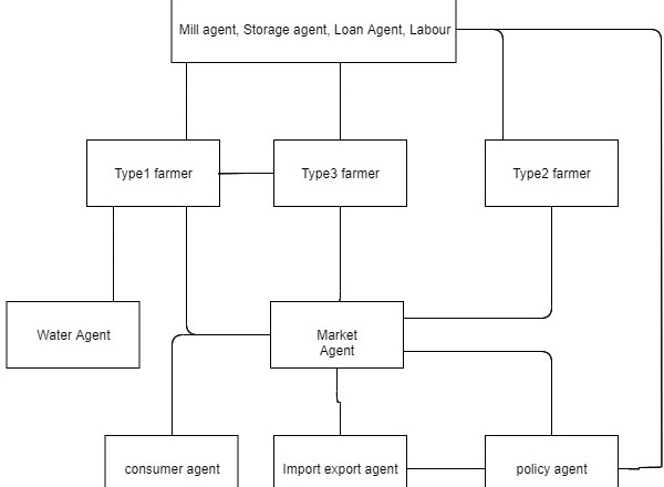
Figure 1. A basic template view of interactions among agents. The interactions of each agent are shown separately later.

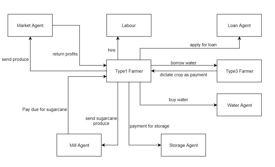
Figure 2. This figure shows how the Type1 farmer interacts with other agents

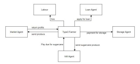
Figure 3. This figure shows how the Type2 farmer interacts with other agents

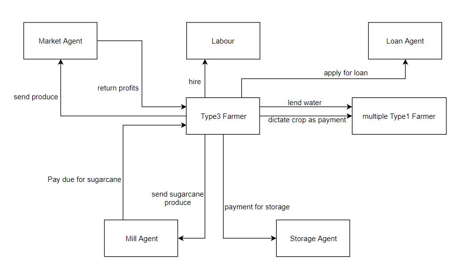
Figure 4. This figure shows how the Type3 farmer interacts with other agents

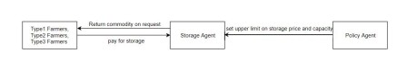
Figure 5. This figure shows how the Storage agent interacts with other agents

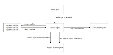
Figure 6. This figure shows how the market agent interacts with other agents

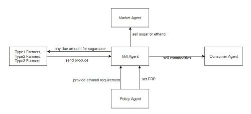
Figure 7. This figure shows how the mill agent interacts with other agents

4. Results

We will see how some of the most common policies implemented by the government affect the system. We also show some alternate policies that give some good results in the simulations.

First we define what is meant by good results. In the simulations we have set 70% of the farmers to be of Type1, 20% as Type2 and remaining as Type3 (India, 2018). We have simulated using 10,000 farmer agents. Now, if the total savings goes below a certain number, a family cannot be sustained, so in that case the farmer “moves out of farming" and finds an alternate source of income. So, in the simulations if a farmer’s savings goes below the cumulative per-person-charge for a family for 4 time steps then the farmer stops farming and moves to a different line of work. Ideally, the number of farmers moving out should be 0 assuming no other external influences, which means farming is sustainable. But, that is not the case, the simulations show that without proper help the number of farmers moving out can go as high as 80-90%. So, in the simulations we use number of farmers moving out as the metric for testing the efficacy of a policy.

We will see how the simulations run for the current real world values for the parameters like FRP, demand and export prices.

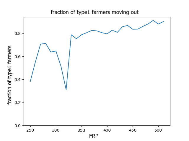
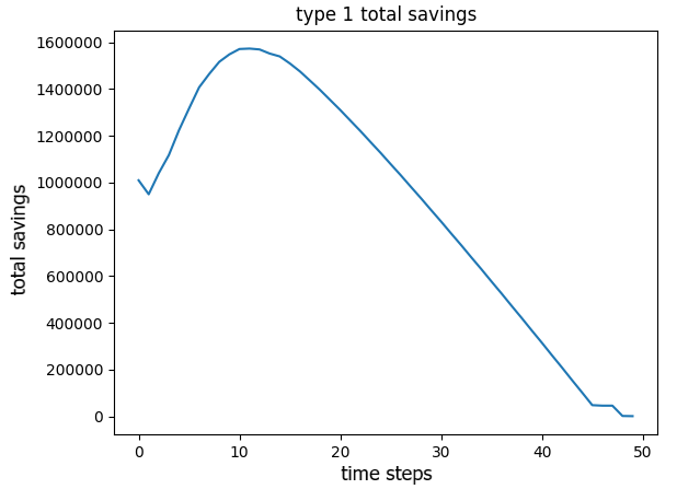
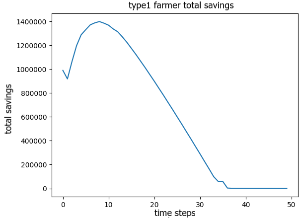
Figure 8. (a) Graph of the number of farmers moving out vs FRP for sugarcane in Rs/Quintal (b) Graph of the savings of Type1 farmers vs time steps when FRP is 220 per Quintal (c) Graph of the savings of Type1 farmers vs time steps when FRP is 480 per Quintal

As we can see from Figure 8, changing the FRP for sugarcane does not help the farmer. Rather higher values of FRP increases the number of farmers moving out of sugarcane farming. This is because, FRP is the initial income expectation. Due to it being high, most of the sugarcane farmers plant sugarcane. Now, if the FRP is low, after the first few time steps, the farmers deem the income unsustainable and stop planting it all together. But with high FRP, the number of time steps before the income expectation falls from FRP to a non profitable income is higher. Even the mill owners keep track of the sugar already existing and hence they do not buy if they have excess sugar. So, when the farmers keep producing sugarcane and the mill owners buy very limited amounts of sugarcane it leads to the farmers dumping sugarcane that makes the situation worse. We can see this effect from Figures 8 and 8. In 2014, sugar price fell to Rs.24 per kg, in the crushing season of 2015, several mills in Uttar Pradesh refused to buy sugarcane from farmers. After the government made it mandatory for mill owners to buy sugarcane from farmers, the arrears of 2016-2017 reached Rs.25.35 billion.

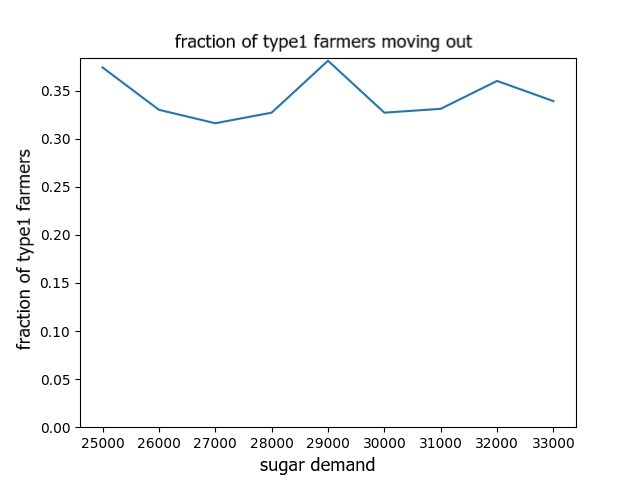
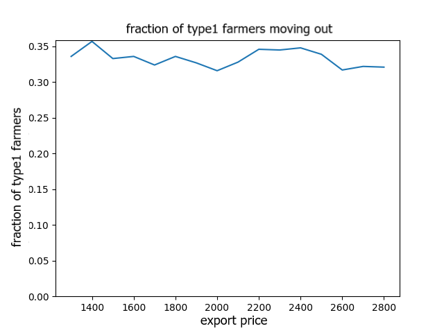
Figure 9. (a) Graph of the number of farmers moving out vs demand of sugar in Quintals (b) Graph of the number of farmers moving out vs export price of sugar in Rs/Quintal

From figure 9 we can see changing the demand is not helpful either, unless the demand is very high. As the price is very low rationally the market simply exports the sugar. But since export prices are low it does not boost incomes which does not help in reducing the stress.

From figure 9, we can see that without much increase in export price not much difference can be seen in the number of farmers exiting from farming. The reason is the same as before. If the export price is significantly higher then most of the produce is exported leading to increased prices which depresses demand and the number of farmers moving out becomes higher.
The increase in storage facilities do not help increase the income of Type1 farmers significantly in general. But there was a significant increase in the case of Type3 farmers. This is not specific for sugarcane farming. Figures 10 and 10 show how the Type1 farmers’ savings and Type3 farmers’ savings changed over the course of time when the storage capacities increased.

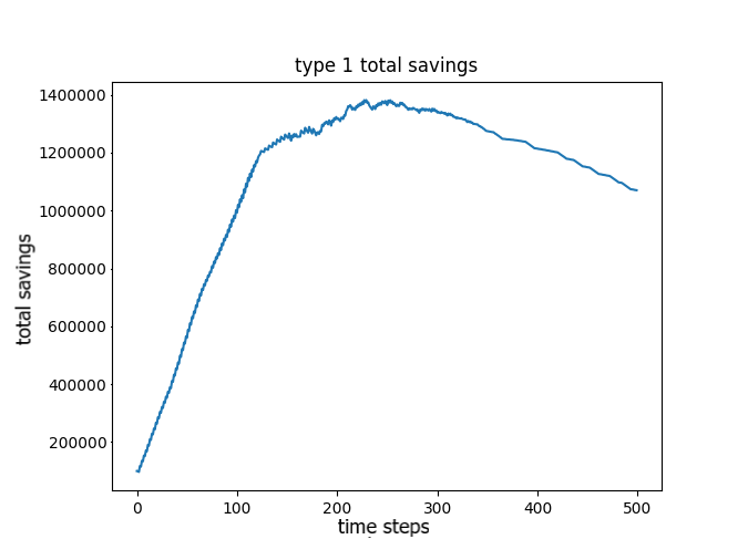
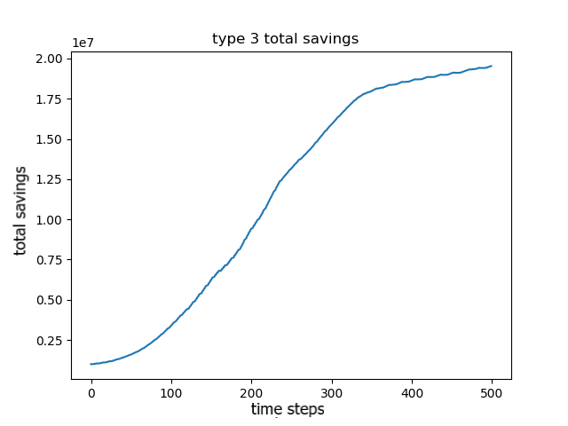
Figure 10. (a) Graph of the savings of Type1 farmers vs Number of time cycles(number of 4 month cycles) (b) Graph of the savings of Type3 farmers vs Number of time cycles(number of 4 month cycles

Below are some simulations that reduced the number of farmers moving out of sugarcane farming:

1. By increasing the requirement of ethanol we can see some substantial improvement in the income of the farmers. Figure 11 and 11 show the number of people moving out of sugarcane farming versus the ethanol requirement for blending. At present blending is only 3.5%. The simulation shows that if blending of 10% is made mandatory, then approximately 50% of the sugarcane farmers will remain in farming. By changing the blend percentage to 20%, 70% of sugarcane farmers will remain in farming. We also tried to see whether changing the price of ethanol helps sugarcane farmers. Figure 11 shows the results.

   

   

   

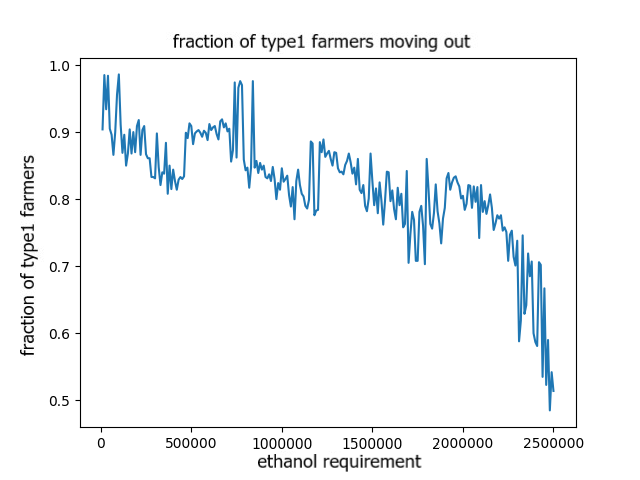
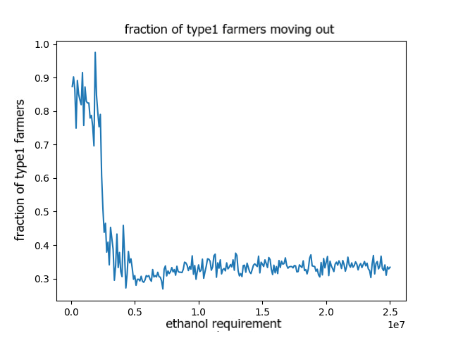
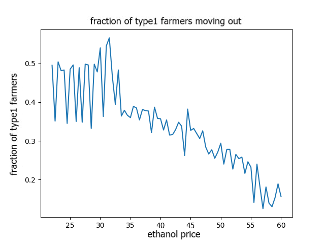
   Figure 11. (a) Graph of the number of farmers moving out vs requirement of ethanol in kilo-litres, (b) Graph of the number of farmers moving out vs requirement of ethanol in kilo-litres with x-axis scale 10 times as (a), (c) Graph of the number of farmers moving out vs price of ethanol in Rs/L

2. Increasing ethanol requirement or increase in ethanol price also leads to stabilization of price of sugar. Due to ethanol business being sustainable sugar production can be controlled, as opposed to converting all the sugarcane to sugar due to the wastage of sugarcane involved. Figure 12 captures this effect. In all the graphs, ‘Price of Type 0’ refers to sugar price.

   

   

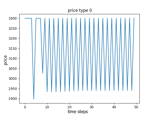
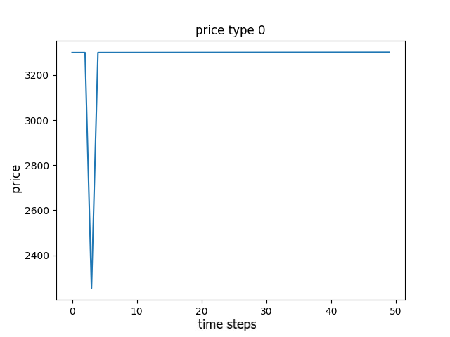
   Figure 12. (a) Graph of price of sugar in Rs/Quintal vs Time cycles when ethanol price is kept as 22 Rs/L. Though the fluctuation may seem huge but the fluctuation is actually small (4 Rs/kg) (b) Graph of price of sugar in Rs/Quintal vs Time cycles when ethanol price is kept as 58 Rs/L.

3. From figure 12, it can be seen that the price does not change a lot. The initial price fluctuation is due to excess sugar produced due to lack of initial demand information for sugar. Because sugar can be stored easily, the amount of sugar in the market can be monitored and the price of sugar kept in check. The increase in ethanol requirement promotes the production of ethanol and hence does not let the store houses be filled with unmanageable amount of sugar.

   

   

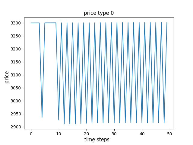
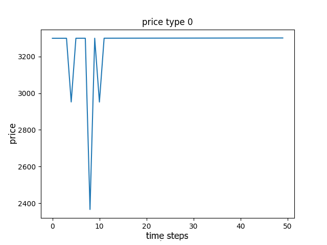
   Figure 13. (a) Graph of price of sugar in Rs/Quintal vs Time cycles when ethanol requirement at is kept at 40,00,00,000 Litres. (b) Graph of price of sugar in Rs/Quintal vs Time cycles when ethanol requirement is kept at 2,20,00,00,000L. From the graph, it can be seen that the price doesn’t change a lot here as well

4. From the figures 13 and 13 we can see that the increase in ethanol requirement can also provide a stabilizing effect on the price of sugarcane. Even at low prices of ethanol, if the demand for ethanol is significant the total profit made by the mill owners is substantial and makes the ethanol business viable. So, similar to the case where the ethanol prices were changed, the sugar production can be manipulated to make the overall sugar and ethanol business profitable.

5. We have also tried to see what happens when farmers are given an alternative crop to sugarcane. With the introduction of one alternative whose price is one third the price of sugar and export price slightly higher than the average price of the new crop (10% more) the situation improves greatly. The main advantage here is that the ratio of people moving out of agriculture becomes approximately 5% which is much better than the best case scenario of ethanol price increase or ethanol requirement increase (which is approximately 20%).

6. The addition of the new crop also has a stabilizing effect on the prices of both crops.

With the introduction of a second crop and alternating the crops the farmer can get better income because by the time the second crop gives a yield the price of sugar goes up and vice-versa.

So, the following are some policy suggestions:

• Increase the ethanol requirement by increasing blending percentage of ethanol with petrol.

• Increase the ethanol price to a value above 55 or 60 Rs/L. This will be a small price to pay if we can treat petrol just as another commodity and apply GST.

• Come up with alternative crops for sugarcane farmers that have a produce price at least 5 times the FRP, export price at least 10% more than the average price offered for the new crop and the yield of at least 5 tonne per acre, which is 10% of the sugarcane yield per acre. For example onions or potatoes.

We have also simulated the policies implemented by Central Government of India regarding sugarcane.
We have simulated 10% ethanol blended with petrol policy by varying the FRP from Rs 270 per Quintal to Rs 500 per Quintal. The ethanol prices used were Rs 51 per litre and Rs 60 per litre, because these were the prices proposed by the Central Government depending on how the ethanol was made in the mills.

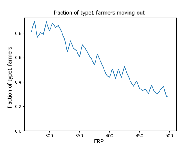
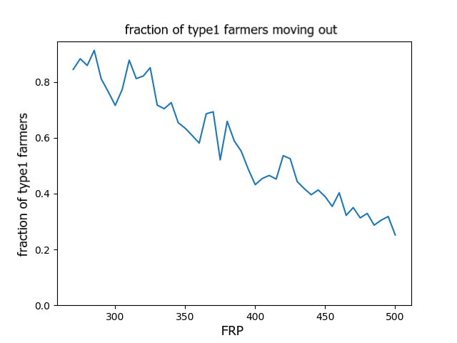
Figure 14. (a) Graph of Farmers leaving sugarcane agriculture vs FRP when ethanol price is Rs 51/litre. (b) Graph of Farmers leaving sugarcane agriculture vs FRP when ethanol price is Rs 60/litre.

From figures 14 and 14, we see that unless the FRP increases the value paid by the mills to the farmers it does not sustain the farmers. From figure 15 we can see even after changing ethanol prices, if the FRP remains the same, it is still not profitable for type1 farmers. But for type3 farmers who have large land holdings, sugarcane farming remains profitable, which can be seen from figure 15.

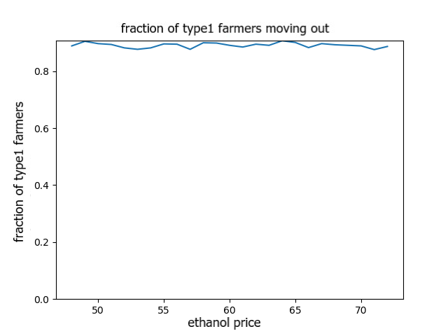
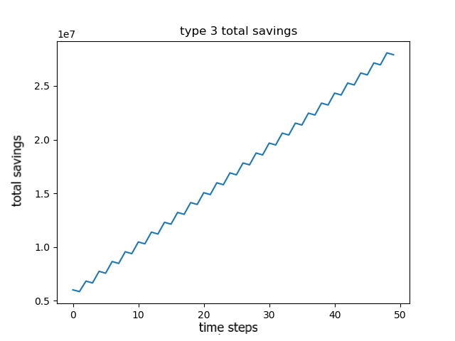
Figure 15. (a) Graph of Farmers leaving the sugarcane agriculture vs ethanol price when FRP is Rs 275/Quintal. (b) Graph of type 3 farmer’s savings vs time cycles when FRP is Rs 275/Quintal and ethanol price is Rs 51/litre.

5. Conclusion

Multi agent systems can be used as a reliable tool to simulate the outcomes of different policies. While the current model is fairly simple it is much easier to build more detailed models with more complex decision processes for agents and richer interactions among agents. More work needs to be done on using Multi-Agent Systems coupled with intelligent learning agents in the socio-economic sector. The behaviour of the agents can be changed and the number of agents can be scaled depending on requirements and resources. Availability of good data and the ability to identify and model all the agents and factors in the real system is the main limitation for this kind of modelling. Assuming the model is valid the simulations show that current policies are not sufficient for improving the livelihood of farmers. The suggested alternatives should be considered and empirically tested.

References

- (1)
- Association (2018) Indian Sugar Mills Association. 2018. World per Capita Consumption of Sugar. https://www.indiansugar.com
- Association (2019) Indian Sugar Mills Association. 2019. The Indian Sugar Industry. https://www.indiansugar.com
- Bar-Yam (1997) Yaneer Bar-Yam. 1997. Dynamics of complex systems. Vol. 213. Addison-Wesley Reading, MA.
- Byrd et al. (2000) Richard H Byrd, Jean Charles Gilbert, and Jorge Nocedal. 2000. A trust region method based on interior point techniques for nonlinear programming. Mathematical Programming 89, 1 (2000), 149–185.
- Department of Agriculture and Welfare (2019) Cooperation Department of Agriculture and Farmer Welfare. 2019. Commodity Profile for Sugar, July, 2019. http://agricoop.nic.in
- Happe et al. (2006) Kathrin Happe, Konrad Kellermann, and Alfons Balmann. 2006. Agent-based analysis of agricultural policies: an illustration of the agricultural policy simulator AgriPoliS, its adaptation and behavior. Ecology and Society 11, 1 (2006).
- India (2016) Open Government Data (OGD) Platform India. 2016. Criteria for classification of marginal, small, medium and large operational holders (farmers) in the country is as under during 2016. https://data.gov.in/
- India (2018) Open Government Data (OGD) Platform India. 2018. State-wise Percentage of Small and Marginal farmers and Women farmers under PMFBY during 2017-18. https://data.gov.in/
- Krejci and Beamon (2012) Caroline C Krejci and Benita M Beamon. 2012. Modeling food supply chains using multi-agent simulation. In Proceedings of the 2012 Winter Simulation Conference (WSC). IEEE, 1–12.
- Kremmydas (2012) Dimitris Kremmydas. 2012. Agent based modeling for agricultural policy evaluation: A. (2012).
- Lobianco and Esposti (2010) Antonello Lobianco and Roberto Esposti. 2010. The Regional Multi-Agent Simulator (RegMAS): An open-source spatially explicit model to assess the impact of agricultural policies. Computers and Electronics in Agriculture 72, 1 (2010), 14–26.
- Lychkina and Morozova (2015) Natalia N Lychkina and Yulia A Morozova. 2015. Agent based modeling of pension system development processes. In SAI Intelligent Systems Conference (IntelliSys), 2015. IEEE, 857–862.
- Motieyan and Mesgari (2018) Hamid Motieyan and Mohammad Saadi Mesgari. 2018. An Agent-Based Modeling approach for sustainable urban planning from land use and public transit perspectives. Cities (2018).
- of Food and Distribution (2019) Department of Food and Public Distribution. 2019. Sugarcane General Policy. https://dfpd.gov.in
- of India (2019) Times of India. 2019. Farmers ask Haryana government to increase sugarcane prices. https://timesofindia.indiatimes.com
- Pyka and Fagiolo (2005) A Pyka and G Fagiolo. 2005. Agent-Based Modelling: A Methodology for Neo-Schumpeterian Economics. The Elgar Companion to Neo-Schumpeterian Economics. H. Hanusch and A. Pyka.
- Saleth (2007) Rathinasamy Saleth. 2007. Water Markets in India: Economic and Institutional Aspects. Vol. 15. 187–205. https://doi.org/10.1007/978-0-585-32088-5_12
- Sivaraman (2016) Madhu Sivaraman. 2016. Government’s Role in India’s Ailing Cold Storage Sector. https://www.cppr.in
- Troost et al. (2015) Christian Troost, Teresa Walter, and Thomas Berger. 2015. Climate, energy and environmental policies in agriculture: Simulating likely farmer responses in Southwest Germany. Land Use Policy 46 (2015), 50–64.