SuperRAENN: A Semi-supervised Supernova Photometric Classification Pipeline Trained on Pan-STARRS1 Medium Deep Survey Supernovae

Abstract

Automated classification of supernovae (SNe) based on optical photometric light curve information is essential in the upcoming era of wide-field time domain surveys, such as the Legacy Survey of Space and Time (LSST) conducted by the Rubin Observatory. Photometric classification can enable real-time identification of interesting events for extended multi-wavelength follow-up, as well as archival population studies. Here we present the complete sample of 5,243 “SN-like” light curves (in g_P1r_P1i_P1z_P1) from the Pan-STARRS1 Medium-Deep Survey (PS1-MDS). The PS1-MDS is similar to the planned LSST Wide-Fast-Deep survey in terms of cadence, filters and depth, making this a useful training set for the community. Using this dataset, we train a novel semi-supervised machine learning algorithm to photometrically classify 2,315 new SN-like light curves with host galaxy spectroscopic redshifts. Our algorithm consists of a random forest supervised classification step and a novel unsupervised step in which we introduce a recurrent autoencoder neural network (RAENN). Our final pipeline, dubbed SuperRAENN, has an accuracy of 87% across five SN classes (Type Ia, Ibc, II, IIn, SLSN-I). We find the highest accuracy rates for Type Ia SNe and SLSNe and the lowest for Type Ibc SNe. Our complete spectroscopically- and photometrically-classified samples breaks down into: 62.0% Type Ia (1839 objects), 19.8% Type II (553 objects), 4.8% Type IIn (136 objects), 11.7% Type Ibc (291 objects), and 1.6% Type I SLSNe (54 objects). Finally, we discuss how this algorithm can be modified for online LSST data streams.

1 Introduction

Time-domain astrophysics has entered a new era of large photometric datasets thanks to on-going and upcoming wide-field surveys, including Pan-STARRS (PS; Kaiser et al. 2010), the Asteroid Terrestrial-impact Last Alert System (ATLAS; Jedicke et al. 2012), the All-Sky Automated Survey for SuperNovae (ASASSN; Shappee et al. 2014), the Zwicky Transient Facility (ZTF; Kulkarni 2018), the Legacy Survey of Space and Time (LSST; Ivezic et al. 2011), and the Roman Space Telescope (Spergel et al., 2015). LSST, to be conducted by the Vera C. Rubin Observatory between 2023 and 2033, is expected to discover roughly one million SNe per year, a more than two orders of magnitude increase compared to the current rate.

Historically, SNe and other optical transients have been classified primarily based on their optical spectra. Class labels are largely phenomenological, dependent on the presence of various elements in the photospheric-phase spectra (see e.g., Filippenko 1997 for a review). SNe, for example, have historically been classified as Type I (equivalent to today’s Type Ia) or Type II based on the absence or presence of strong hydrogen Balmer lines, respectively. As the number of events increased, further classes were created to account for the increased diversity (e.g., Uomoto & Kirshner 1985). Type Ib and Type Ic designations were created to indicate the presence and absence of helium, respectively. Today, semi-automated software such as GELATO (Harutyunyan et al., 2008), SNID (Blondin & Tonry, 2007) and Superfit (Howell et al., 2005) are used to match SN spectra to a library of previously classified events to determine the spectroscopic class. More recently, Muthukrishna et al. (2019) utilized a convolutional neural network to classify SN spectra.

However, spectroscopic follow up remains an expensive endeavor, taking up to an hour on 8-meter class telescopes to classify a single object given the depth wide-field surveys can now achieve. As a result, only $\sim 10\%$ of the $\sim 10^{4}$ transients currently discovered each year are spectroscopically classified. Spectroscopic follow up is not expected to significantly increase when the LSST commences, meaning that only $\sim 0.1\%$ of events will be spectroscopically classified.

Given the growing rate of discovery and limited spectroscopic resources, classification of transients based on their photometric light curves is becoming essential. Luckily, the phenomenological labels often correspond to unique underlying processes that are also encoded in the light curve behavior. For example, while Type Ia SNe are spectroscopically classified by strong Si II absorption and lack of hydrogen, these features distinctly originate from the thermonuclear detonations or deflagrations of carbon-oxygen white dwarfs, which also lead to specific light curve evolution (Hillebrandt & Niemeyer, 2000). Generally, unique progenitor system and explosion mechanisms likely lead to other observable features, some of which are captured in broadband optical light curves. Said features allow transients to be classified into their traditional subclasses (based on spectroscopy and photometry) using only their broadband, optical light curves.

There is a growing literature on light curve classifiers that rely on data-driven and machine learning algorithms. Most studies use supervised learning, in which the training set consists of SNe with known classes (e.g., Lochner et al. 2016; Charnock & Moss 2017; Boone 2019; Villar et al. 2019; Möller & de Boissière 2020). However, SN classification can benefit from semi-supervised methods, in which the training set contains both labelled and unlabelled SNe. The unlabelled set is used to better understand low-dimensional structure in the SN dataset to improve classification. Richards et al. (2012), for example, created a diffusion map (a nonlinear dimensionality reduction technique) based on light curve similarities in shape and color using unlabelled data from the Supernova Photometric Classification Challenge (SPCC; Kessler et al. 2010). They use the diffusion map to extract 120 nonlinear SN features from each labelled SN, which are then used to train a random forest classifier. More recently, Pasquet-Itam & Pasquet (2018) introduced the PELICAN classifier, also trained on synthetic SPCC data. PELICAN uses a convolutional autoencoder to encode nonlinear SN features and a set of fully connected neural network layers to classify the full set of simulated SPCC light curves as Ia or non-Ia SNe.

Here we introduce a new semi-supervised classification method for SNe, which utilizes a recurrent autoencoder neural network (RAENN). This method is uniquely trained on real (rather than simulated) data from the Pan-STARRS1 Medium Deep Survey (PS1-MDS) and is optimized for general SN classification (as opposed to Ia versus non-Ia classification). Our method has been trained on a combination of 557 spectroscopically-classified SNe and 2,328 additional SN-like events. We then use RAENN and hand-selected features with a random forest to classify the PS1-MDS sample of 2,315 previously unclassified SN-like transients with host galaxy spectroscopic redshifts. We publish the full set of light curves and associated labels for community use. We present an open source code listed on the Python Package Index as SuperRAENN (Villar, 2020). A companion paper, Hosseinzadeh et al. (2020, hereafter H20), presents and compares photometric classifications of the same dataset using an independent classification method (following the supervised methods of our previous work in Villar et al. 2019).

The paper is organized as follows. In §2, we review the PS1-MDS and associated sample of SN-like transients. In §3 we introduce the RAENN architecture and training procedure. We present the classification results and discuss implications in §4 and §5, respectively. We conclude in §6. Throughout this paper, we assume a flat $\Lambda$CDM cosmology with $\Omega_{M}=0.307$, and $H_{0}=67.8$ km s^-1 Mpc^-1 (Ade et al., 2014).

Figure 1: Peak apparent $r$-band magnitude of the full SN-like dataset (grey), objects used in our unsupervised method (orange) and the spectroscopic sample (blue). The spectroscopic dataset is roughly one magnitude brighter than the full dataset.

Figure 2: Histogram of the redshifts of the full SN-like dataset (grey line; 4,055 objects), the subset of host redshift measurements for objects used in our unsupervised learning algorithm (black line;2,885 objects), and the subset with spectroscopic classification (colored lines; 557 objects). The shaded grey region represents the summed, spectroscopically classified objects. The full sample and spectroscopic distribution peak at $z\approx 0.25$, although the spectroscopic sample has an additional peak near $z\approx 0.1$. At $z\gtrsim 0.75$, the spectroscopic sample is limited to SLSNe.

2 The PS1-MDS Supernova Sample

PS1 is a wide-field survey telescope located near the summit of Haleakala, Maui with a 1.8 m diameter primary mirror and a 1.4 gigapixel camera (GPC1) (Kaiser et al., 2010). PS1-MDS, one of several PS1 surveys (Chambers et al., 2016), was conducted between July 2009 and July 2014. It consisted of 10 single-pointing fields, each of approximately 7.1 deg², with a pixel-scale of $0.^{\prime\prime}25$. The survey was conducted in five broadband filters (Stubbs et al., 2010; Tonry et al., 2012) with a nominal cadence of $3$ days per filter in four filters ($g_{\mathrm{P1}}r_{\mathrm{P1}}i_{\mathrm{P1}}z_{\mathrm{P1}}$), and a $5\sigma$ limiting magnitude of $\approx 23.3$ per visit. In practice, Scolnic et al. (2018) finds a cadence of roughly $6-7$ days per filter. In general, PS1-MDS observed a field in $g_{\mathrm{P1}}$ and $r_{\mathrm{P1}}$ on the same night, followed by $i_{\mathrm{P1}}$ and then $z_{\mathrm{P1}}$ on subsequent nights. PS1-MDS also included observations in the $y_{\mathrm{P1}}$-band, primarily near full moon and with a shallower $5\sigma$ limiting magnitude of $\approx 21.7$. Due to the poor cadence and shallow depth, we do not use the $y_{\mathrm{P1}}$ data here.

During its 5-year survey, PS1-MDS discovered 5,243 SN-like objects, defined as events with at least three observersations with a signal-to-noise ratio (SNR) $>4$ in any filter and no previous detection within the survey (Jones et al., 2018, 2019). We obtain data for these events via the PS Data Processing System (Magnier et al., 2016, 2016; Waters et al., 2016). The photometric pipeline is based on photpipe (Rest et al., 2005, 2014) with improvements made in Scolnic et al. (2018). Images and templates, used for image subtraction, are re-sampled and aligned to match a “skycell” in the PS1 sky tessellation. Image zeropoints are determined by comparing point spread function (PSF) photometry of stars to PS1 stellar catalogs (Chambers et al., 2016). PS1 templates are convolved to match nightly images and then subtracted using HOTPANTS (Becker, 2015). For each event, a flux-weighted centroid is calculated and forced PSF photometry is performed at the centroid. Finally, a nightly zeropoint is applied.

Of the 5,243 SN-like objects, 4,090 host galaxies were targeted through a concerted observational effort. To identify the most likely host galaxy for each SN, we used the galaxy size and orientation-weighted R-parameter from Sullivan et al. (2006), as outlined in Jones et al. (2017). The majority (3,321 objects) were observed using the Hectospec multifiber instrument on MMT (Fabricant et al., 2005; Mink et al., 2007). Additional host redshifts were obtained with the Anglo-Australian Telescope (AAT; 290 objects), the WIYN telescope (217 objects), and the Apache Point Observatory 3.5m telescope (APO; 5 objects). Host galaxies selected for follow-up were largely unbiased in terms of transient properties (e.g., we did not prioritize SNe based on luminosity, color or amount of additional followup). Additional host redshifts were obtained from archival survey data: 2dFGRS (Colless et al., 2003), 6dFGS (Jones et al., 2009), DEEP2 (Newman et al., 2013), SDSS (Smee et al., 2013), VIPERS (Scodeggio et al., 2018), VIMOS (Le Fèvre et al., 2005), WiggleZ (Blake et al., 2008) and zCOSMOS (Lilly et al., 2009).

We use the RVSAO package (Kurtz & Mink, 1998a) to determine the spectroscopic redshifts through cross-correlation with galaxy templates. We use the standard RVSAO galaxy templates (including spiral and elliptical galaxies and quasars), as well as galaxy templates provided by SDSS (Adelman-McCarthy et al., 2007). We quantify the quality of the template matches using the Tonry & Davis (1979) cross-correlation parameter, $R_{\mathrm{CC}}$. Following Jones et al. (2017), we remove host galaxies with $R_{\mathrm{CC}}<4$, ensuring that the vast majority ($\approx 98$%) of the remaining galaxies have accurate redshift measurements. This cut removes 1,084 SNe with redshift measurements.

To ensure that our final set of redshift measurements is robust, we identify a subset of spectra to be manually validated. Of the remaining redshifts which we initially estimate using RVSAO, we accept the redshift of the best-matching template without visual inspection if the median redshift estimate across templates is equal to both the most-likely redshift and the mode of the template matches and more than two templates match this redshift estimate. We (VAV and GH) visually inspected $\sim 600$ redshift spectra to ensure that our final redshift estimates are as accurate as possible. In total, 2,487 redshifts (of 3,056 redshift estimates with $R_{\mathrm{CC}}\geq 4$) match the most-likely redshift provided by RVSAO. Of the remaining hosts, we remove 393 redshift estimates which we could not validated manually. A total of 145 redshifts ($\sim 4$%) which were measured manually do not match the median or mode of the RVSAO redshift estimates. The galaxy spectra and further details are presented in H20.

We additionally remove events with $z<0.005$, which are unlikely to be SNe given the peak absolute magnitudes (e.g., Chornock et al. 2010). We visually inspect the light curves which have quasar-like hosts (based on template matching) or which overlap with the host galaxy’s center. We remove events which are clearly variable over multiple seasons and lack a transient spectrum. Our final sample includes 2,885 transients with redshifts measurements (from the hosts or transients themselves), including spectroscopically-identified SNe.

2.1 Spectroscopic versus Photometric SN Sample

Approximately 10% of the PS1-MDS transients were spectroscopically observed in real time throughout the survey, without a specific selection function (although brighter objects were more likely to be targeted). For this work, we limit our spectroscopic sample (557 objects) to five potential classes:

1. Type I SLSNe (17 objects), which are thought to arise from the birth of highly magnetized neutron stars (Quimby et al., 2007; Chomiuk et al., 2011; Nicholl et al., 2017)

2. Type II SNe (94 objects; including Type IIP and Type IIL SNe), which arise from red supergiant progenitors

3. Type IIn SNe (24 objects), powered by the interaction the SN ejecta with pre-existing circumstellar material (e.g. Smith et al. 2014)

4. Type Ia SNe (404 objects), which are the thermonuclear explosions of white dwarfs

5. Type Ibc SNe (19 objects), which arise from the core-collapse of massive stars that have lost their hydrogen (Ib) and helium (Ic) envelopes. Due to the small sample size we consider Type Ib and Type Ic SNe as a single class.

The SLSN and Type Ia SN light curve samples have been previously published in Lunnan et al. (2018) and Jones et al. (2017), respectively. Model fits to the Type II light curves were presented in Sanders et al. (2015). For four objects, the transient spectra yield a reliable redshift but an ambiguous classification. A fifth object, PSc130816, has previously been identified as both a Type IIP/L SN (Sanders et al., 2015) and a Type IIn SN (Drout, 2016). We do not include these five objects in our spectroscopic sample. An additional 15 objects are spectroscopically identified but do not fall in on of our five classes, including two tidal disruption events (TDEs), a lensed Type Ia, a Type Ibn, a Type Iax and ten fast evolving luminous transients (FELTs). All except the TDEs are included in our photometric sample for training purposes, but not included in our spectroscopic sample. These objects are discussed in more detailed in §5.1

Our photometric sample contains 2,315 objects with host galaxy spectroscopic redshifts, that are independent of the 557 SNe which are spectroscopically classified. We refer to the union of the photometric and spectroscopic samples (the full set of 2,885 events), as the “complete” photometric dataset. We summarize the PS1-MDS SN-like objects, their associated hosts and redshift information in Table 1. We also specify which SNe are used in the supervised/unsupervised portions of our classification algorithm.

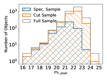
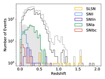
Our spectroscopic dataset is brighter than our complete photometric dataset. As shown in Figure 1, the spectroscopic sample has a median peak $r$-band magnitude of $\sim-21$ mag, about 1 magnitude brighter than the photometric sample. We directly compare the redshift distributions in Figure 2. The spectroscopic sample peaks at a slightly lower redshift compared to the photometric dataset($z\approx 0.27$ versus $z\approx 0.35$), with a tail extending to $z\approx 1.0$. The lack of confident high-redshift measurements is likely due to the key spectroscopic lines shifting out of the optical and due to the peak absolute magnitudes of most SNe falling below our limiting magnitude. The mismatch between the spectroscopic and photometric samples may translate to biases in our classification pipeline, which we explore in more detail in § 5. The complete $griz$ light curves of our sample are available on Zenodo (Villar et al., 2020).

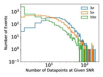
We explore the overall data quality of our sample in Figure 3, finding that the majority of events have $\sim 20$ data points across all filters with signal-to-noise ratios of $\gtrsim 3$. Given a typical SN duration of a month and our typical cadence of a few days, we expect the majority (but not all) SNe to have fairly complete light curves.

Figure 3: Histogram of the number of SN light curves with $N$ data points with SNR of $\geq 3$ (blue), $\geq 5$ (orange), and $\geq 10$ (green) from the complete sample of SN-like objects (5,243 events). Most events have $\approx 10-20$ $3\sigma$ data points, with only a handful having $>100$ points.

3 A Semi-supervised Classification Pipeline

About 10% of our SN sample is spectroscopically classified. Traditional supervised classification methods are strictly limited to this subset of our data, as they require labelled SN examples. However, information about SN subtypes exists as substructure in the unlabelled dataset as well. For example, SN classes may be clustered in duration and luminosity (e.g., Kasliwal 2012; Villar et al. 2017). Because we would like to leverage the information in both the labelled and unlabelled subsets of the training set, we use a recurrent autoencoder neural network (RAENN) paired with a random forest classifier for a semi-supervised classification approach. In this section, we describe the complete algorithm and training process.

Our pipeline is composed of three steps: (1) a pre-processing and interpolation step using Gaussian processes (GP); (2) an unsupervised step in which we train a RAENN on the complete photometric set (labelled and unlabelled); and (3) a supervised step in which we train a random forest on the spectroscopically labelled set of SNe. The complete pipeline, dubbed SuperRAENN (Villar, 2020), is available via GitHub.

3.1 Pre-processing with Gaussian Processes

Figure 4: Examples of three spectroscopically classified SNe and their associated GP-interpolated light curves in the four PS1 filters ($g$: green; $r$: red; $i$: orange; $z$: purple). Solid lines represent the mean GP prediction, while the shaded regions represent the $1\sigma$ estimated uncertainties.

We generate and pre-process absolute magnitude light curves before extracting features. We correct each light curve for Milky Way reddening using the extinction map of Schlafly & Finkbeiner (2011). We estimate and normalize the absolute magnitude using the measured host redshift:

$$\begin{split}M_{\mathrm{norm}}=m-5\log_{10}(d_{\mathrm{L}}/10\mathrm{pc})\\ +2.5\log_{10}(1+z)-m_{\mathrm{lim}}-A_{\lambda}\end{split}$$ (1)

where $m_{\mathrm{lim}}$ is a chosen limiting magnitude, which we take to be $m_{\mathrm{lim}}=25$. This value is dimmer than the $5\sigma$-limiting magnitude of PS1-MDS. We choose a dimmer magnitude to ensure that even marginal detections will be included in the light curve. We perform the re-normalization so that the GP mean will be zero (i.e., the light curve will be zero when no data is available). Finally, we correct all light curves for time-dilation based on the measured redshifts. We do not attempt to make a wavelength-dependent $k$-correction to the rest-frame data given the complicated, diverse, and time-evolving spectral energy distributions (SEDs) of the various SN types.

We do not correct the SN light curves for host galaxy reddening. The intrinsic reddening of SNe adds an additional scatter in our feature space. Correcting for host galaxy reddening would require estimating both the color excess and dust law, which is not possible given our current dataset.

The PS1-MDS light curves are irregularly sampled across the four filters (see §2 for the PS1 observing strategy). The architecture of the RAENN does not require uniformly sampled light curves. However, it does require that each observation is made in all four filters. For example, if an observation is made in $g$-band, we need to provide interpolated values for $riz$-bands for that time.

To interpolate the $griz$ light curves, we fit a GP using the open-source Python package George (Foreman-Mackey, 2015). GPs are a non-parametric model that has been previously used to interpolate and classify SN light curves (see e.g., Lochner et al. 2016; Revsbech et al. 2018; Boone 2019). GPs define a prior over a family of functions, which is then conditioned on the light curve observations. A key assumption is that the posterior distribution describing the light curve is Gaussian, described by a mean, $\mu(\vec{t})$, and a covariance matrix, $\Sigma(\vec{t})$, given by $\Sigma_{i,j}=\kappa(\vec{x_{i}},\vec{x_{j}})$ with kernel $\kappa$. We use a 2D squared exponential kernel to simultaneously fit all four filtered light curves:

$$\begin{split}\kappa(\vec{t_{i}}\vec{t_{j}}\vec{f_{i}}\vec{f_{j}};\sigma,l_{t}l_{f})=\sigma^{2}\exp\Big{[}-\frac{(t_{i}-t_{j})^{2}}{2l_{t}^{2}}\Big{]}\\ \times\exp\Big{[}-\frac{(f_{i}-f_{j})^{2}}{2l_{f}^{2}}\Big{]}\end{split}$$ (2)

where $f$ is an integer between 0 and 3 that represents the $griz$ filters, and the parameters $l_{t}$ and $l_{f}$ are characteristic correlation length scales in time and filter integer, respectively. This fitting process accounts for the measured data uncertainties, making it robust to low-confidence outliers.

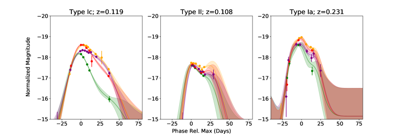
We independently optimize the kernel parameters for each SN using the minimize function implemented in scipy, with initial values of $l_{t}=100$ days and $l_{f}=1$. We find that our choice of initialization values has little effect on the resulting best fit. We find that $l_{t}$ is typically about one week, and $l_{f}$ is typically $2-3$, indicating that the filters are highly correlated. Examples of the GP interpolation for Type Ia, Type Ic and Type II SNe are shown in Figure 4. The GP is able to produce reasonable interpolated light curves even in cases with sparse and noisy data and provide reasonable error estimates.

A similar GP method was implemented by Boone (2019) to classify a variety of SN types in the Photometric LSST Astronomical Time-series Classification (PLAsTiCC; The PLAsTiCC team et al. 2018; Kessler et al. 2019) dataset. Instead of an integer, Boone 2019 used the rest frame central wavelength of each filter for each object. We avoid this added layer of complexity because the $k$-corrections and time-evolving SN spectral energy distribution (SED) change the weighted central filter wavelength. However, the simple 2D kernel still allows the four bands to share mutual information.

Our light curves contain several years of data, most of which are non-detections. To limit our input data, we keep datapoint (of any significance) within 100 days of peak flux (in whichever filter is brightest). For ease of optimization, the light curves need to contain the same number of data points. The data must be a consistent size during the back-propagation step of optimization for the RAENN for each iteration (see next section). Our longest light curve contains 169 data points, so we pad all light curves to match this length. We do so by appending a value dimmer than the estimated absolute limiting flux (we use $m_{\mathrm{lim}}=25$) to 100 days after the last detection in the light curve.

We note that using luminosity-based light curves (rather than magnitudes) is an alternative pre-processing choice. Luminosity-based light curves would remove the need to re-normalize the light curves to a chosen limiting magnitude. We find that using luminosity-based light curves results in worse performance of the RAENN, likely due to the orders-of-magnitude differences in scale between events.

3.2 Unsupervised Learning: A Recurrent Autoencoder Neural Network (RAENN)

Figure 5: Diagram of the RAENN architecture. The pre-processed GP-interpolated light curves are fed into the encoder, which encodes the light curve into an encoding vector. This vector is then repeated, and new time values are appended to each copy. The final light curve is then predicted at each new time value. The RAENN is trained by comparing the input light curve with the predicted light curve. The values from the encoded layer are inputted into the random forest as features and used to classify the SN light curves.

To extract unique features from the complete (unlabelled and labelled) PS1-MDS photometric sample, we construct a RAENN, inspired by the work of Naul et al. (2018), who uses a similar method to classify variable stars.

Neural networks are a class of machine learning algorithms that use many latent layers to model complex functions. These and other machine learning algorithms are becoming increasingly common in astronomy (see Ntampaka et al. 2019 for an overview). Autoencoders (AEs, Kramer 1991) are a class of neural network architectures that learn a compressed representation of input data. By training an AE to return the original data given a limited set of variables, it learns an “encoded” version of the data.

In astrophysics, AEs have been used for feature-learning in galaxy spectral energy distributions (SEDs, Frontera-Pons et al. 2017), image de-noising (Ma et al., 2018; Lucas et al., 2018), and event classification (Naul et al., 2018; Pasquet et al., 2019). AEs are also increasingly being used in the astrophysics literature for dimensionality reduction (see e.g., Ralph et al. 2019 and Portillo et al. 2020 for recent examples).

Here, our model is designed to address several concerns of SN light curves: (1) the temporal irregularity of data; (2) data across multiple filters; and (3) streaming data that update on a given cadence. The last point is not a concern for our PS1-MDS archival dataset, but it will become important as LSST comes online and discovers thousands of SNe nightly.

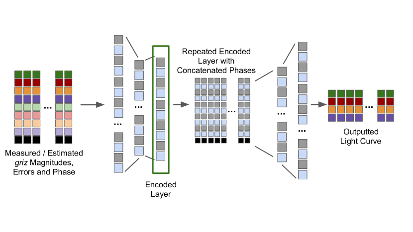
The RAENN uses the GP light curves as input, by codifying the light curves as matrices of size $9\times T_{0}$, where $T_{0}=169$, as described in the previous section. The $9$ values are: one time value, relative to maximum (in whichever filter is brightest); four magitude values ($griz$) at that time; and four magnitude uncertainties. Recall that the magnitude values are either measured or estimated from the GP. For the uncertainties, we use the $1\sigma$ errors for the measured points. For the GP points, we use a large error of 1 mag. We note that the GP produces estimates errors, but we find that, in practice, using this larger error bar leads to better performance. We leave exploration of utilizing error bars to future work. We emphasize that, while $T_{0}=169$ for training, the RAENN architecture allows a user to input a light curve of any size without needing to pad the light curve.

The RAENN architecture is divided into an encoder and a decoder. Our encoder is a series of fully-connected layers that decrease in size until the final encoded layer with size $N_{E}$ (i.e., the number of neurons used to fully encode the SN light curve). We note that $N_{E}$ is a free parameter of our model that needs to be optimized. Similarly, the fully-connected layer has $N_{N}$ neurons, where $N_{N}>N_{E}$ and is also a tunable parameter. Following the encoded layer, the decoder half of the architecture mirrors the encoder with increasing layer sizes.

A novel feature of our architecture is the inclusion of a repeat layer immediately after our final encoding layer (the layer of size $N_{E}$). In this layer, we repeat the encoded version of the light curve $T_{N}$ times. To each copy, we append the time of each data point, relative to peak brightness in one filter (whichever filter happens to be brightest). One way to view the purpose of this layer is to imagine the autoencoder as two functions. The first function (the encoder) takes in the original data points, including observation times, and outputs a set of $N_{E}$ values. This is similar to the idea of taking a light curve and fitting it to a model with $N_{E}$ free parameters. A second function (the decoder) takes in a set of $N_{E}$ values and $T_{N}$ times to generate a light curve at the $T_{N}$ times. This architecture allows us to generate a light curve at different $T_{N}$ times; e.g., interpolated or extrapolated light curves, which is further explored in §5. In this work, we choose $T_{N}=T_{0}$; namely, we repeat the encoded values to match the original light curve length.

Our autoencoder utilizes gated recurrent neurons (GRUs; Cho et al. 2014; Rumelhart et al. 1988). In addition to the typical hidden weights that are optimized during training, recurrent neurons have additional weights that act as “memory” of previous input. GRUs in particular utilize an update value (called a gate) and a reset gate. The values of these neurons determine how the current and previous input affect the value of the output. With each light curve data point, the gates become updated with new information that informs the next prediction. This class of neurons is useful for our light curves with various numbers of observed data points. Our GRU neurons use the $\tanh$ activation functions with a hard sigmoid for the gate activation function.

Our RAENN is implemented in Keras (Chollet, 2015) with a Tensorflow backend (Abadi et al., 2016). A diagram of the architecture is shown in Figure 5, and is outlined as follows:

1. Input Layer: Input light curve of size $T_{0}\times 9$ with each $griz$ data point labelled with a time (1 value) in days relative to light curve peak (4 values) and an uncertainty (4 values).

2. Encoding Layer: Encoding layer with $N_{N}$ neurons, where $N_{N}$ is a hyperparameter.

3. Encoded Layer: Encoded light curve with $N_{E}$ neurons, where $N_{E}$ is a hyperparameter.

4. Repeat Layer: Layer to repeat encoded light curve to match with new time-array, with size $T_{0}\times N_{E}$.

5. Concatenate Layer: Layer to concatenate new times to encoded light curve, with size $T_{0}\times(N_{E}+1)$.

6. Decoding Layer: Decoding layer with $N_{N}$ neurons.

7. Decoded Layer: $T_{0}\times 4$ decoded $griz$ light curve.

To optimize the free parameters (the weights) of the RAENN model, we must define a loss function. Our loss function is a simple mean square error function:

$$\mathcal{L}=\sum_{i=0}^{N}\frac{\Big{[}F_{i,\mathrm{True}}(t,f)-F_{i,\mathrm{Predicted}}(t,f)\Big{]}^{2}}{N},$$ (3)

where $F$ is the SN flux as a function of time $t$ and filter $f$. Although we feed unvertainties into the network, we find that excluding flux errors in our loss function substantially improved the ability of the RAENN to match the input light curves. We minimize our loss function using the gradient descent-based optimizer, Adam (Kingma & Ba, 2014), finding an optimal learning rate of $10^{-4}$, which is a typical value.

Figure 6: Confusion matrices for the full set of 557 spectroscopically classified SNe. In the bottom panel, we include only objects where the maximum probability is $\geq 0.7$ (438 events). Left panels: Completeness-based confusion matrices, in which each row is normalized to equal one. Completeness quantifies how much of a spectroscopic class the classifier has correctly classified. Right panels: Purity-based confusion matrices, in which each column is normalize to equal one. Purity quantifies how much a photometric class is comprised of the true spectroscopic class. By restricting our classes to the high-confidence objects (bottom panels), both our completeness and purity increase.

Figure 7: Top: Cumulative fraction of the spectroscopic SN sample as a function of classification confidence (left) and number of $>5\sigma$ data points (right), grouped by spectroscopic class. Misclassifications are marked with an “x”. Middle: Cumulative fraction of the spectroscopic SN sample, grouped by photometrically-identified class. As expected, most misclassifications occur at low-confidence. At our chosen high-confidence cutoff ($p>0.7$), we find that the samples are largely pure. Bottom: Cumulative fraction of the photometric SN sample, grouped by photometrically-identified class. The distributions based on classification confidence follow a similar trend to those seen in the spectroscopic sample, with Type Ia SNe and SLSNe having the highest fraction of high-confidence events. However, the photometric set has significantly more points on average when compared to the spectroscopic dataset.

We randomly split our unlabeled dataset into training (2/3) and test (1/3) sets. We optimize the number of neurons in both the encoding and decoding layers (fixed to be the same number, $N_{N}$) and the number of encoding neurons ($N_{E}$) through a grid search, allowing $N_{N}$ to vary from 20 to 160 in intervals of 20, and $N_{E}$ to vary between 2 and 24 in intervals of 2. We find that, when optimizing over final classification F1-score (defined below), purity and completeness, our results are relatively insensitive to $N_{E}$ and $N_{N}$ for values of $N_{E}\sim 10$ and $N_{N}\sim 100$. For our final model, we use $N_{E}=8$ and $N_{N}=120$, which is not our optimal model but a representative model. Utilizing our optimal model without creating a valid test set (in addition to a training and validation set) would likely overestimate performance. Given our limited dataset, we are unable to properly optimize our hyperparameters and thus present representative results. We note that $N_{N}$ is slightly below the maximum number of data points in our set of light curves (where the longest light curve has 169 observed data points). The number of encoding neurons $N_{E}$ is similar to the number of free parameters for the analytical model used in Villar et al. (2019) to capture the shape of a single-filter SN light curve.

We contrast our architecture with methods from Naul et al. (2018) and Pasquet et al. (2019), who present similar methodologies. Naul et al. (2018) uses a similar GRU-based RAENN to classify variable stars with unevenly sampled light curves in one filter from the All Sky Automated Survey Catalog of Variable stars (Pojmanski, 2002). The flux and time since last observation ($\Delta t$) is sequentially read into the recurrent layers. The same time array is fed into the decoder for output. In our case, we feed in a time series across four filters and give a time array relative to peak rather than relative to the previous data point. This is more natural in our problem, in which the SNe have a clear beginning and end, versus the periodic signals of variable stars. Additionally, our architecture allows us to give the decoder a different time series to allow for interpolation or extrapolation of the data.

Pasquet et al. (2019) uses a semi-supervised method to classify simulated SN light curves from the SPCC (Kessler et al., 2010). They use an AE with convolutional layers by transforming the light curves into “light curve images” (see Pasquet-Itam & Pasquet 2018). Rather than interpolate the light curves, Pasquet et al. (2019) applies a mask to filters that are missing data at a certain time. In contrast, we interpolate our light curves but assign interpolated values a large uncertainty of 1 mag, as explained above. We found that the method of transforming light curves into images and masking across four filters led to unstable training and poorer performance. This is likely due to the large data gaps in the real PS1-MDS light curves, compared to the high-cadence (2-days for each filter) simulated light curves of SPCC. Since the LSST data are expected to more closely resemble the PS1-MDS light curves than the SPCC simulated events, we expect our method to be more robust in a real-life application.

Figure 8: Completeness and purity confusion matrices, generated from classifying the spectroscopic dataset using only RAENN features and leave-one-out cross-validation. Even without additional features, the classifier performs similarly to other simulation-based classifiers such as those presented in Muthukrishna et al. (2019) and Boone (2019).

3.3 Supervised Learning: Random Forest Classifier

As a final step, we use the encoded light curves as features for a supervised classification method. Following Villar et al. (2019), we train a random forest (RF) classifier on the PS1-MDS spectroscopically classified SNe, including the RAENN encodings as features.

In addition to the encoding (8 features), we use the following 36 features based on the GP-interpolated light curves:

• The $griz$ rise times in the rest frame, calculated 1, 2, and 3 mag below peak (12 features).

• The $griz$ decline times in the rest frame, calculated 1-, 2- and 3-magnitudes below peak (12 features).

• The $griz$ peak absolute magnitudes (4 features)

• The median $griz$ slope between 10 and 30 days post-peak in observer frame. This area was chosen by eye to specifically help the model differentiate between Type II and Type Ibc SNe (4 features).

• The integral of $griz$ light curves (4 features).

We measure these values from the GP-interpolated light curves rather than the decoded light curves. The decoded light curves are, at best, approximations of the GP-interpolated light curves. Therefore, using them would only result in noisier features. The decoded light curves are necessary, however, as a means to train the RAENN to extract the $N_{E}$ encoding neuron values. We note that for some features, e.g., the rise and decline times, the feature values are heavily dependent on the GP extrapolation in cases where there is no measured data. Including GP errors in the supervised portion of our analysis could help capture this intrinsic uncertainty in the underlying light curve, but we leave that exploration to future work.

These features were chosen through trial-and-error while optimizing classification accuracy. We find that inclusion of all features leads to our optimal classification accuracy, although we do explore how well our classifier performs with the RAENN features alone in the following section.

We pass these features through a RF classifier, utilizing 350 trees in the random forest and the Gini-information criterion. The number of trees was determined based on trial-and-error optimization. To counteract the imbalance across the five spectroscopic classes, we tested several algorithms to generate synthetic data to augment our training set. Following Villar et al. 2019, we use a Synthetic Minority Over-sampling Technique (SMOTE; Chawla et al. 2002) and a multivariate Gaussian (MVG) fit. We additionally test using a Kernel Density Estimate (KDE) of the training set, using a Gaussian kernel with bandwidth equal to 0.2 (or 20% of the whitened feature standard deviation). We find that the MVG with a halved covariance matrix performs best. We test our classifier using leave-one-out cross validation, in which we remove one SN from the sample, oversample the remaining objects by generating new objects using the MVG, and then apply the trained RF to the single, removed event and recording the result. For each object, our RF reports probabilities associated to each class, which are calculated using the fraction of trees which vote for each class. We take the class with the highest probability as the predicted SN type.

4 Classification Results

Figure 9: Bottom: Confusion matrices for a simpler Type Ia SN versus non-Ia (CCSN) classification, generated by collapsing the complete confusion matrices.

There are several metrics to measure the success of a classifier. We focus on three metrics: the purity, completeness and accuracy. We define the three, calculated for a single class, below:

$$\begin{split}\mathrm{Purity}&=\frac{\mathrm{TP}}{\mathrm{TP}+\mathrm{FP}}\\ \mathrm{Completeness}&=\frac{\mathrm{TP}}{\mathrm{TP}+\mathrm{FN}}\\ \mathrm{Accuracy}&=\frac{\mathrm{TP}+\mathrm{TN}}{\mathrm{TS}}\end{split}$$ (4)

where TP (FP) is the number of true (false) positives, TN (FN) is the number true (false) negatives, and TS is the total sample size. We optimize the hyperparameters of our classifier using the F1-score, defined here as the class-averaged harmonic mean of the purity and completeness.

4.1 Spectroscopic Sample

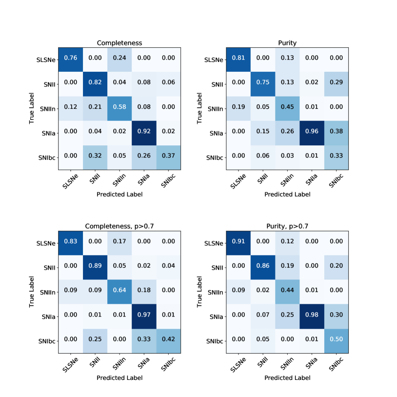
We visualize the completeness and purity of the spectroscopic sample using confusion matrices in Figure 6. A confusion matrix compares our RAENN label (horizontal axis, in the case of the completeness matrix) with the spectroscopic label (vertical). Results are shown for leave-one-out cross validation, in which one event is removed from the sample for training and the trained model is applied to the left out event. As with Villar et al. (2019), we find that our classifier performs best for Type Ia SNe (92% completenss), SLSNe (76%), and Type II SNe (82%), and worst for Type Ibc SNe (37%). Our class-averaged classification completeness is 69% across the 5 SNe types. This is worse than the performance of Villar et al. (2019), who find a class-averaged completeness of 80%. Our class-averaged purity is 66%, again slightly worse than the average purity of 72% found in Villar et al. (2019). When limiting the sample to only objects in which the classification probability is $\geq 0.7$ (a total of 438 objects), we find that our performance increases, with a class-averaged completeness of 75% and a class-averaged purity of 74% with a loss of 20% of the sample size.

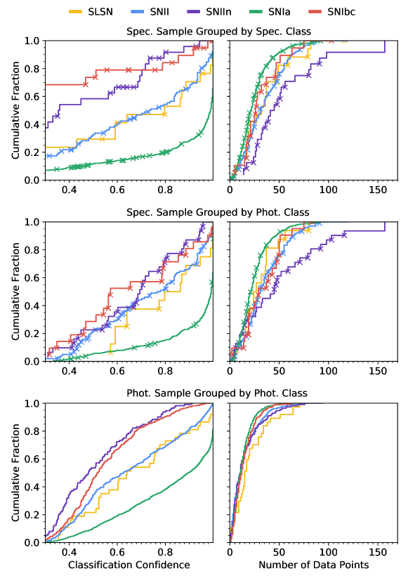
Next, we explore the classification confidence reported by our algorithm. The confidence estimates are directly outputted by the RF. With larger datasets, one can calibrate the outputted uncertainties using e.g., an additional logistic function. Given our small dataset, we do not perform any additional calibration. In Figure 7 we plot the cumulative fractions of SNe in our training set, grouped by their spectroscopic and photometric classifications. The majority of high-confidence objects are Type Ia SNe, with nearly half of the spectroscopic Type Ia SNe having a confidence (p$>0.98$). Similarly, half of the SLSNe have high confidence identifications ($p>0.8$). Type Ibc SNe and Type IIn SNe have the lowest confidence on average, with the majority of events having $p<0.5$. This is likely reflective of the fact that Type Ibc and Type IIn SNe span a wide range of observed properties, including overlap with Type Ia SNe.

Figure 7 also indicates the misclassified objects. Ideally, we want our misclassifications to largely occur in low-confidence objects. This is the case for SLSNe, Type Ia SNe and Type II SNe. For Type IIn and Type Ibc SNe, the misclassifications occur even for high-confidence events. This indicates that for Type Ia, Type II and SLSNe, misclassifications are likely tied to data quality. In contrast, misclassifications of Type IIn and Type Ibc SNe seem to be due to intrinsic overlap of the classes in feature-space with other SNe (mainly Type Ia SNe).

We additionally attempt to sort events based on the number of data points, rather than classification confidence (see the right column of Figure 7). Our photometric dataset has, on average, fewer $>5\sigma$ datapoints compared to our spectroscopic dataset ($\sim 15$ versus $\sim 30$ data points on average). Because of this mismatch and the lack of a strong correlation between number of points and classification confidence, we do not further explore how cutting sparse light curves affects our final classification accuracy.

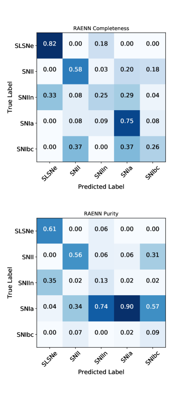
We next turn our attention to the performance of our classifier when constrained to only data-driven (RAENN) features. Using the same set of RAENN features without any additional information, we produce the confusion matrices shown in Figure 8. We find a class-averaged completeness of 53%, approximately 20% worse than including the additional features. The overall breakdown is similar to our final confusion matrix, with the worst-performing classes being Type Ibc and Type IIn. We find that our RAENN-only classification is more inclined to label events as Type Ia SNe, likely a bias from the fact that our SN dataset used to train the RAENN is highly dominated by Type Ia SNe. If we run our classification algorithm without the RAENN features, we find that SuperRAENN performs similarly (slightly worse), implying that the RAENN has not picked up on uniquely helpful features independent from our hand-selected feature set. To be clear: the intent of RAENN is not necessarily to outperform hand-selected features but to create model-independent features in real time. In this work, we determine final classifications with the RAENN and hand-selected features to provide the highest confidence photometric classifications. Improvements to classifications based solely on RAENN features is left to future work.

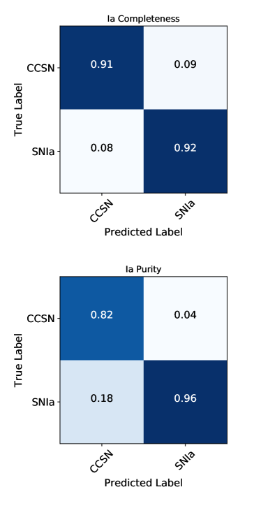
While not optimized for Type Ia versus non-Type Ia SN classification, we explore how well our classifier (using the full set of features) performs when we collapse the confusion matrix into just two classes. In Figure 9, we show the completeness and purity confusion matrices for Type Ia versus non-Ia (CCSN) classifications, finding $\approx 90$% completeness and $>80$% purity in both classes.

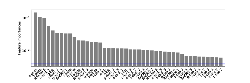
The random forest classifier allows us to measure the relative “importance” of the 44 features used to classify the SNe. We define importance as the decrease in the Gini impurity, which accounts for how often a feature is used to split a node and how often a node is reached in the forest (Breiman et al., 1984). We show the importance of each RF feature in Figure 10, along with the measured importance for a Normal random variable. The peak magnitudes and decline rates are the most important features for classification. However, the RAENN features also have significant influence on the final classifications, with two RAENN features appearing in the top ten important features.

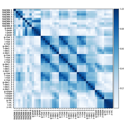
The feature importance unfortunately loses some quantitative meaning if the features are correlated, which is the case with our features. When two features are highly correlated, one may be arbitrarily measured as more important, so the general trends are more meaningful than precise order. We show the magnitudes of the feature correlations in Figure 12 to better understand the underlying correlations. There are clear correlations between features derived in multiple bands (e.g., the peak magnitude in $g$-band is highly correlated to that in $r$-band). However, we also see correlations between the RAENN features and the more traditional light curve features. About half of the RAENN features seem strongly correlated with the peak magnitudes, while two others seem well-correlated with rise and decline times. A more detailed exploration of the physical interpretation of the RAENN feature-space may be worthwhile but is beyond the scope of this work.

Figure 10: Feature importance (grey). The blue horizontal line shows the importance measure for a normally-distributed random variable; features at or below this line can be considered largely unimportant to the final classification. In our case, all featured are considered important by the RF.

Figure 11: A sample of SNe from our photometric sample, sorted by low (left column) versus high (right column) confidence and photometrically identified SN class (rows). Here we show only $>3\sigma$ detections and otherwise show magnitudes as upper limits (triangles). Low-confidence in classification appears to be both due either poor data quality or confusion between multiple classes.

Figure 12: Absolute values of the covariance matrix of the various features used in our classification method, where darker blue represents a stronger absolute correlation. Unsurprisingly, the same features derived from different bands (e.g., the peak $g$-band flux versus the peak $r$-band flux) are highly correlated. The RAENN features are also correlated to the physically-motivated parameters, with some being strongly correlated to peak magnitudes, some to rise and decline times, and some to the post-peak slope.

4.2 Classifying the Complete Photometric Dataset

Figure 13: Breakdown of SN subclasses in the spectroscopic and photometric samples. There is a significantly smaller fraction of Type Ia SNe in our photometric sample (orange) versus our spectroscopic sample (blue), implying we have misclassified Type Ia SNe as CCSNe. If we limit our photometric sample to the high-confidence ($p>0.7$) events (green), the class breakdowns are better aligned. Using our confusion matrix, we can correct the photometric class breakdown for known biases (see text for details; red), which also better aligns our class breakdowns. Finally, we compare our results to the ZTF Bright Transient Survey, finding good agreement between the spectroscopic class breakdown and corrected photometric class breakdown (Fremling et al., 2019).

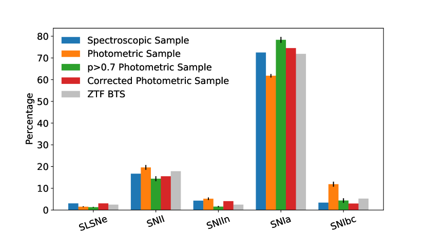
We apply our trained classification algorithm to the PS1-MDS dataset of SN-like transients that pass our quality cuts described in § 2. We report the probabilities of each class type for each light curve in Table 2. Error bars for each class probability are calculated by running the trained RF classifier 25 times with unique random seeds. We show the class breakdown of the complete photometric set (2,885 SNe) in Figure 13. Excluding the spectroscopic sample, we present 2,315 new SNe with 1435 (61.9%) Type Ia SNe, 459 (19.9%) Type IIP SNe, 272 (11.7%) Type Ibc SNe, 112 (4.8%) Type IIn SNe, and 37 (1.6%) SLSNe. Of these, 1,311 are high-confidence ($p>0.7$) photometric classifications. A cumulative plot of the confidences grouped by each photometric class is shown in Figure 7; the distribution of these probabilities largely match the spectroscopic sample.

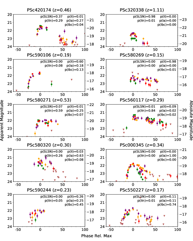
A sample of SNe from each photometric class is shown in Figure 11, including high- and low-probability examples. For the low-probability examples, it seems that even well-sampled light curves can have low confidence scores, likely because the features of their light curves reside on a region of feature space in which various SN classes reside.

The redshift distributions of the new, photometrically-classified events is roughly consistent with that seen in the spectroscopic sample (Figure 2), with Type Ibc peaking at $z\sim 0.19$, Type II peaking at $z\sim 0.21$, Type Ia and Type IIn peaking at $z\sim 0.42$ and SLSNe peaking at $z\sim 0.58$.

We compare the overall photometric breakdown of SN types to that of the ZTF Bright Transient Survey Fremling et al. (2019), which spectroscopically classified 761 SNe with peak $g$- or $r$-band magnitude of $<18.5$. Fremling et al. (2019) find that their magnitude-limited survey breaks down into 72% Type Ia SNe, 16% “normal” Type II SNe (Type IIP/L), 3% Type IIn SNe (including their Type IIn and SLSN-II category), 5% Type Ibc SNe, and 1.6% Type I SLSNe. This is a similar breakdown found in our spectroscopic sample. Comparing to our photometric set, we find a slightly higher fraction of Type II and Type IIn SNe and a lower fraction of Type Ia SNe (all within $\sim 20$% of the ZTF BTS values), as shown in Figure 13. For our high-confidence ($p>0.7$) sample (also shown in Figure 13), our class breakdowns are closer to those of our spectroscopic and the ZTF BTS sample, with a slight over-abundance of Type Ia SNe ($\approx 78$%). Based on our understanding of how our classifier performs on the training set, we can understand the biases present (e.g., that some spectroscopic Type Ibc SNe are classified photometrically as Type Ia SNe). We can use these known biases, encoded within the confusion matrices, to correct our class breakdown. Mathematically, this is calculated as the dot product of the purity matrix and our original class breakdown. Applying this correction to the photometric dataset, the class breakdown is well aligned with the breakdown of our spectroscopic sample, as shown in Figure 13. This study should not be used to rigorously study the observational breakdown of SN classes; however, the fact that our $p>0.7$ sample is in relatively good agreement with the ZTF BTS provides some evidence that our photometric sample is correctly labelled.

5 Discussion

5.1 Classification of Other Transients

Our algorithm assumes that every SN belongs in one of five classes: SLSNe, Type II SNe, Type IIn SNe, Type Ia SNe and Type Ibc SNe. Yet what does our algorithm do for transients which do not fall in these five classes? Here we address this question for a number of spectroscopically classified extragalactic transients. We summarize the photometric classification for these rare transients in Table 3.

Drout et al. (2014) presented a sample of ten extragalactic transients discovered with PS1-MDS with redshift measurements which rise too rapidly to be powered solely with $56$Ni. Following Rest et al. (2018), we refer to these as FELTs. FELTs have a broad range of peak magnitude (-16 $\gtrsim M\gtrsim$ -20), which is reflected in the distribution of photometric classifications. Of these ten objects, six objects have “high confidence” ($p>0.7$) classifications in one of our five categories: four of which are Type Ia SNe and two of which are Type II SNe. The other four objects are classified as low confidence Type Ia (one object), Type II (two objects) and Type Ibc (one object). As expected, the higher-luminosity objects are those classified as Type Ia, while the lower-luminosity objects are classified at Type II. The majority of objects have Type Ibc as their second-highest classification. Based on this analysis, FELTs are likely a (small) contaminant of both Type II and Type Ia SNe in our sample, and our algorithm would need to be retrained to specifically classify FELTs.

Two known TDEs were discovered in PS1-MDS: PS1-10jh (PSc040777, Gezari et al. 2012 and PS1-11af (PSc120170, Chornock et al. 2014. Both objects are classified as Type IIn SNe with $p\sim 0.8$ and $p\sim 0.6$, respectively. This makes intuitive sense, as the light curves tend to be long-lived and bright like some Type IIn SNe. Both objects have Type Ia and Type II as their next most likely classifications. Based on these, it may be possible to search for TDEs in our sample within the photometric Type IIn sample.

We highlight four other SNe which do not fit in our five categories. PS1-10afx (PSc080333) is a lensed Type Ia SN (Chornock et al., 2013; Quimby et al., 2014), which peaks at -22 mag. We classify PS1-10afx as a high probability ($p\sim 0.9$) SLSN. PS1-12sk (PSc370290) is a Type Ibn SN (Sanders et al., 2013) which peaks at $M\sim-19$. We classify PS1-12sk as a low probability Type Ia ($p\sim 0.6$) or Type IIn ($p\sim 0.4$). We classify PS1-12sz (PSc370330) as a likely IIb SN using SNID; PS1-12sz peaks at $M\sim-18.5$. We photometrically classify this object as a low probability Type Ibc ($p\sim 0.6$). Finally, SN 2009ku (PS0910012) is a spectroscopically identified Type Iax (Narayan et al., 2011) which peaks at $M\sim-18.5$. We classify this object as a low probability Type Ia ($p\sim 0.5$) or Type Ibc ($p\sim 0.3$).

5.2 Potential Biases

As discussed in § 2, our spectroscopic sample is somewhat brighter and at a lower redshift than our test set. This difference may introduce biases in our final classifications, although this effect should be minimal considering the small ($\sim 1$ mag) difference between the two sets. De-redshifting the SNe removes some of this bias, by removing knowledge of the underlying redshift as a feature. The relative fractions of SN subtypes may evolve with redshift as host properties change (see e.g., Graur et al. 2017 for an exploration of the correlations between host properties and SN type). Our spectroscopic and photometric sets differs most greatly at $z\gtrsim 0.5$ (see Fig. 2). In this redshift range, average host metallicity is not expected to drastically shift (Lilly et al., 2003), implying a small potential bias. A separate bias may arise from the fact that our photometric sample relies on a measured spectroscopic redshift. At higher redshift, our galaxy redshift measurements become increasingly uncertain as dominant emission lines shift out of the optical band and intrinsically dim hosts fall below our observational limits. In contrast, rest-frame UV features of SNe (especially SLSNe) remain in the optical band, making it easier to confidently measure a distance from SNe spectra. In the future, this problem can be mitigated with photometrically derived host galaxy redshifts.

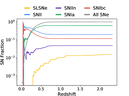
As expected, the relative observed fraction of SN subtypes evolves with redshift due to the magnitude limit of the survey. We trace this evolution in Figure 14. We show the cumulative fraction (integrating from $z=0$) of each subclass as a function of redshift. Each subclass peaks in order of luminosity function. The dimmest subclass, Type II SNe, dominates the sample for $z<0.3$, peaking near $z\sim 0$.

Using the high redshift ($z>0.75$) sample, we can test if redshift information is playing an unwanted role in our training. The spectroscopic sample at $z\gtrsim 0.75$ is solely made up of SLSNe; however, we do not expect all high-$z$ objects to be SLSNe. Given a typical limiting magnitude of $m_{\mathrm{r,lim}}\sim 23.3$, the corresponding absolute magnitude is $\sim-20$ at $z=0.75$. At this sensitivity, we expect to find SLSNe, Type IIn SNe and potentially bright Type Ia SNe (if the limiting magnitude is slightly deeper). For $z>0.75$, we find that our photometric sample (a total of 28 SNe) is 68% SLSNe, 18% Type IIn SNe and 14% Type Ia SNe (with all Ia SNe occurring at $z<0.85$), implying our classifier has not learned to simply classify all high-$z$ events as SLSNe. The high-$z$ Type Ia SNe, in particular, have noisy light curves which peak at $M\sim-20$.

Figure 14: Observed SN subclass cumulative fraction as a function of redshift (colored) and the overall cumulative distribution (grey).

5.3 Comparison to Other Works

We first compare our results to H20, which extends the work of Villar et al. (2019) to classify the PS1-MDS photometric sample using features extracted from analytical fits to the light curves. Overall, H20 (and Villar et al. 2019) achieve better performance at the cost of a more computationally-expensive feature extraction method. We agree with 74% of the photometric classifications of H20. If we compare the top two labels, the algorithms agree on 95% of classifications. Indeed, often the top two classification choices are flipped for either algorithm, occurring most often with Type II/Ibc SNe and Type IIn/Ia SNe. We find stronger agreement if we exclude objects with low classification confidence; namely, using only $p>0.7$ in both algorithms, our classifications agree 84% of the time (with 1,597 objects remaining after the cut, i.e., a loss of $\sim 50$% of the sample). The agreement increases further for even higher probability cuts of $p>0.8$ ($>0.9$), with 88% (92%) agreement with 1249 (888) objects remaining. Most classification disagreements lie in the Type Ibc/IIn categories, which have low confidence classifications. We find that our algorithm is more likely to classify SNe as Type Ia, likely a bias built into the unsupervised step of training on the complete dataset (which is dominated by Type Ia SNe). A more detailed comparison of these two results is provided in H20.

Villar et al. (2019) discusses the difficulty in comparing our results to the broader literature. In short, previous works have largely focused on Type Ia versus CCSN classification (e.g., Ishida & de Souza 2013; Jones et al. 2017; Brunel et al. 2019) or have been trained and tested on simulated data (e.g., Kessler et al. 2010; Muthukrishna et al. 2019; Möller & de Boissière 2020). In the case of Type Ia versus CCSN classification, we achieve an accuracy of $\approx 92$%, similar to (but somewhat worse than) specialized classifiers (Jones et al., 2017; Brunel et al., 2019). When comparing to works based on simulated data, we caution that not all simulated datasets are suitable for multi-class SN classification. In particular, the Supernova Photometric Classification Challenge (SNPCC) training set (Kessler et al., 2010) lacks the SN diversity necessary to accurately train classifiers and will lead to artificially promising results. PLAsTiCC (The PLAsTiCC team et al., 2018; Kessler et al., 2019) is better suited for this task, and we encourage future work to be built on this dataset or the PS1-MDS dataset presented here.

We next compare our results to Jones et al. 2017, who presented a PS1-MDS sample of 1,169 likely Type Ia SNe, focusing on Type Ia versus non-Ia classification. Jones et al. 2017 used four classification algorithms: the template-matching algorithm PSNID (Sako et al., 2011), a nearest neighbor approach using the PSNID templates; an algorithm based on fitting light curves to SALT2 templates (Guy et al., 2007); and a method, GALSNID (Foley & Mandel, 2013), which only utilizes host galaxy properties. Jones et al. (2017) similarly removed objects with unreliable host redshifts and potential AGN hosts, but unlike our analysis they removed objects at $z>0.75$. Of their 1,169 identified Type Ia SNe, only 1,046 SNe pass our quality cuts to be classified in this work. For these, we find 95% agreement. Of the remaining 48 SNe, we identified Type Ia as the second highest choice in 24 cases. Of the remaining 24 cases, 15 have low Type Ia probabilities ($p<0.8$ from Jones et al. 2017) or classification probabilities based entirely on host galaxy. It is worth noting that our classifier, similar to Jones et al. (2017), achieves 96% purity in Type Ia SNe, making it likely usable for cosmological studies (Jones et al., 2018).

We compare our results to those trained on PLAsTiCC – in particular, Boone 2019; Muthukrishna et al. 2019 and Gabruseva et al. 2020. These classifiers present average completenesses of $\approx 0.88$ for SLSNe (higher than our score), $\approx 0.5$ for Type II/IIn SNe (lower than our averaged Type II/IIn score), $\approx 0.92$ for Type Ia SNe (similar to our score), and $\approx 0.46$ for Type Ibc SNe (similar to our score given low-number statistics). These results are based on simulated data which lack the complexity of real data, so it is encouraging that our algorithm performs similarly or outperforms these works. It would be interesting and useful to the community to know how these algorithms perform on the PS1-MDS dataset, but we leave this for future work.

Figure 15: Examples of a Type Ia SN (top row), Type II SN (middle row) and Type Ibc SN (bottom row). Filled points represent observations used to generate the RAENN model (colored lines), while empty points are the full data set to guide the eye. In the right-most column, we show the root-mean-squared (RMS) error as a function of SN phase, as more data are being included in the RAENN model. Interestingly, the RMS reaches $\sim 1$ near peak for all SNe shown. We emphasize that the RAENN model has been optimized to classify complete SN light curves rather than partial light curves.

5.4 RAENN Architecture: Limitations and Benefits

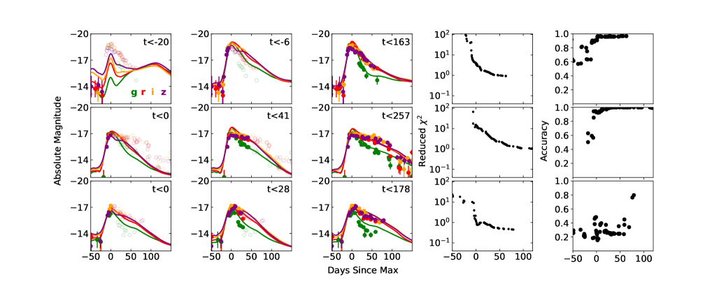
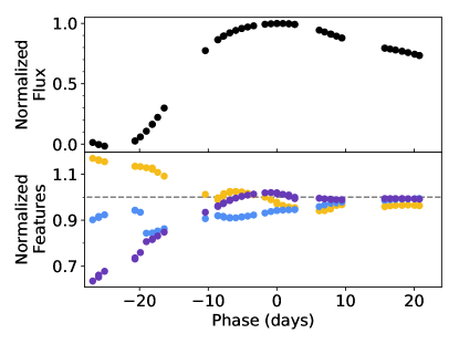
We now turn to the architecture of the RAENN itself and its use in future surveys. The recurrent neurons allow our neural network to generate light curve features that can be updated in real time, in addition to extrapolating and interpolating light curves. We highlight the accuracy of the RAENN light curve model as a function of light curve completeness in Figure 15. We track how well the RAENN is able to both model the complete light curve and accurately classify the SNe with limited data by providing a partial light curve into the RAENN. For each step, we hold the other features (e.g., peak luminosity and duration) constant. This is not a completely robust method, as some features (e.g., decline time) cannot be measured before peak. We leave the optimization of SuperRAENN for real time data streams to future work. We find that SuperRAENN performance drastically improves post-peak, but that it can provide accurate classifications and light curves somewhat before peak. To explore why SuperRAENN improves near-peak, we track how the RAENN features change as the light curves evolve. In Figure 16, we plot the values of representative encoding values of a Type Ia SN. The encodings vary smoothly until settling on the correct final values $\sim 10$ days post-peak.

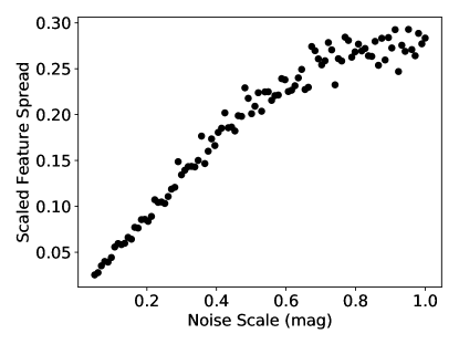
The ability of the RAENN to extrapolate light curves without built-in physical assumptions allows it to search for anomalous events in real time for the purpose of spectroscopic and multi-wavelength follow-up. Given the millions of events expected from LSST, it is essential to search for unexpected or previously unknown physical effects that. One concern is that our algorithm is potentially not robust to noisy live-streaming data; in other words, our algorithm must be able to distinguish between anomalous data and noisy data. We check the stability of our encoded values as a function of scaled white noise by adding white noise to a light curve. We then use our RAENN to encode the noisy light curve and record the scatter of the encoded values. We report the results of this test in Figure 17, in which we show the scaled scatter of the encoded values as a function of the magnitude of the injected noise. The scatter grows linearly with noise; however, even with one magnitude of scatter added to the light curve, the overall scatter of the encoded values only increases to 30% of the overall spread of class’s features. This implies that the RAENN is largely robust to noise.

Several steps need to be taken to allow our architecture to work on streaming data. First, we use phases relative to maximum light, which will be unavailable during the rise of the SN. A shift to a time measurable early in the light curve, like time of first detection, will allow the RAENN to otherwise perform as designed. Similarly, the features utilized during the supervised portion of our classifier rely on the full light curve being available. All features can be estimated from extrapolated RAENN light curves or a new set of features may be used on streaming data. Finally, although not necessary, our RAENN could output uncertainties on the SN light curves by converting the network into a variational AE, which is designed to simultaneously find an encoding space and uncertainties on the encoded data. This more complex architecture would likely require a larger training set to be reliable. Finally, we note that an algorithm like RAENN could be used in conjunction with an active oracle (a software which recommends new observations to improve classification) such as REFITT (Sravan et al., 2020), in order to actively optimize classification accuracy.

6 Conclusions

Deep learning-based classifiers are becoming increasingly important for classification of archival SN light curves. In this paper we present a novel, semi-supervised approach to light curve classification, which utilizes spectroscopically labelled and unlabelled SN data from the PS1-MDS. Our key conclusions are as follows:

1. We present the light curves of 5,243 SN-like events discovered with PS1-MDS.

2. We present the spectroscopic classifications of 557 SNe, including 17 Type I SLSNe, 94 Type II, 24 Type IIn, 404 Type Ia and 19 Type Ibc SNe.

3. We measure and report the spectroscopic redshifts for 2,885 SN-like events used in our unsupervised training set.

4. We present a new, open source photometric classification algorithm, SuperRAENN. SuperRAENN uses a semi-supervised approached and novel neural network architecture to classify irregularly-sampled SN light curves.

5. Using SuperRAENN, we extract learned, nonlinear features from the sparse light curves. We use these features and others to classify the complete set of 2,885 SN-like objects in the PS1-MDS dataset with host galaxy redshifts.

6. We achieve high (87%) accuracy for our spectroscopically labelled sample. We find best performance for SLSNe, Type Ia, and Type II SNe due to their distinctive regions of feature space. We find worst performance for Type Ibc SNe, likely due to the small sample size (just 19 events) and their significant overlap with Type Ia SNe and the subset of rapidly-declining Type II SNe (formerly, IIL).

7. Compared to previous studies, we find that our general classifier performs as well or can outperform classifiers trained on synthetic data sets.

8. We perform simple tests for classification bias and method robustness to noise, finding our method robust to both.

In addition to these key results, we highlight several lessons learned from this study. We find that both Type IIn and Type Ibc classes suffer from poor accuracy likely due to substantial overlap with Type Ia SNe in feature space. This finding has also been shown in Villar et al. (2019) and H20, implying this is a general problem for classifiers. Additionally, rare transients, e.g. FELTs, abnormal Type Ia classes, etc., can be hidden as high-confidence events in another class or low-confidence events across several classes. Adapting pre-existing classifiers to new classes should be taken on a case-by-case basis. Finally, we find that a mixture of hand-selected and data-driven (in our case, RAENN) features can improve classification accuracy, but hand-selected features seem to generally out perform data-driven features.

Finally, we note that several modifications to our presented classifier will allow it to work with live, rather than archival, data streams such as ZTF and LSST. We perform simple tests and find that our classifier performs optimally around peak, although we have not optimized for this purpose. Finally, the RAENN architecture may also be utilized to search for anomalous events in real time. We plan to explore this in future work.

Figure 16: Top: Normalized, GP-interpolated $r$-band light curve of a spectroscopically-classified Type Ia SN. Bottom: Representative set of three (orange, purple, blue) normalized AE features as a function of SN phase. To generate these features, we run the light curve data through the RAENN up to a certain phase. As shown, the values vary smoothly and then settle on the final values about one week post-peak.

Figure 17: Average spread of the RAENN features for a spectroscopic Type Ia SN as a function of light curve noise. For every noise scale, we run 100 simulations, adding random noise to the light curve. We then track the average spread of each parameter. We scale this spread by the total spread in the Type Ia class. Even with an injected error of 0.5 mag, the spread in the RAENN feature space only reaches 30% of the total spread throughout the Type Ia class in feature space, implying the method is robust to noise.

Table 1: SNe Properties

Object	PSc ID	IAU Name	CBET	SN RA	SN Dec	Milky Way	SN Type	Redshifta	Host RA	Host Dec	Num.	Telescopeb/	Unsup.d	Sup.e
Name				(deg.)	(deg.)	E(B-V)			(deg.)	(deg.)	Pointsc	Source
PS1-0909006	PS0909006	SN 2009ks	Rest et al. (2009)	333.9503	1.1848	0.0426	SNIa	0.284	-	-	19	Gem-N	Y	Y
PS1-0909010	PS0909010	SN 2009kt	Rest et al. (2009)	37.1182	-4.0789	0.0256	SNIa	0.27	-	-	20	Gem-N	Y	Y
PS1-0910012	PS0910012	SN 2009ku	Rest et al. (2009)	52.4718	-28.0867	0.0073	SNIax	0.079	-	-	40	Gem-S, NOT, Magellan, Gem-S	Y	N
PS1-0910016	PS0910016	SN 2009kx	Rest et al. (2009)	35.3073	-3.91	0.0219	SNIa	0.23	-	-	10	Gem-N	Y	Y
PS1-0910017	PS0910017	SN 2009kv	Rest et al. (2009)	35.2775	-5.0233	0.0221	SNIa	0.32	-	-	15	Gem-N	Y	Y
PS1-0910018	PS0910018	SN 2009kz	Rest et al. (2009)	35.667	-4.0273	0.0242	SNIa	0.265	-	-	11	Gem-N	Y	Y
PS1-0910020	PS0910020	SN 2009kw	Rest et al. (2009)	54.5975	-28.2533	0.013	SNIa	0.242	-	-	13	Gem-S	Y	Y
PS1-0910021	PS0910021	SN 2009ky	Rest et al. (2009)	53.62	-27.9084	0.0081	SNIa	0.256	-	-	20	Gem-S	Y	Y
PS1-10a	PSc000001	-	-	52.4531	-29.075	0.009	SNII	0.071	52.4536	-29.0744	13	2df	Y	Y
PS1-10aa	PSc010046	-	-	162.9188	58.1822	0.0115	-	0.039	162.9188	58.1822	21	WIYN	N	N
PS1-10aaa	PSc070003	-	-	333.0415	0.7193	0.0479	-	0.1376	333.0414	0.7194	63	NED, SDSS	Y	N
PS1-10aab	PSc070004	-	-	335.0863	0.524	0.0641	-	-	335.088	0.5244	31	-	N	N
PS1-10aac	PSc070039	-	-	334.6541	0.6184	0.0587	-	0.3933	334.6538	0.6186	28	MMT	N	N
PS1-10aad	PSc070048	-	-	241.0171	54.1988	0.0088	-	0.423	241.017	54.1988	15	MMT	Y	N

Note. — A complete, machine-readable version of this table is available in the online version.

a. Redshift estimate from either the transient spectra or host galaxy spectra.

b. Telescope used to acquire galaxy or SN spectra.

c. Number of $>5\sigma$ datapoints in light curve.

d. Included in unsupervised training set. These objects have reliable host redshift estimates.

e. Included in supervised training set.

Table 2: SNe classification

Event Name	pSLSN	pII	pIIn	pIa	pIbc
PSc000001	$0.00_{0.00}^{0.00}$	$1.00_{0.00}^{0.00}$	$0.00_{0.00}^{0.00}$	$0.00_{0.00}^{0.00}$	$0.00_{0.00}^{0.00}$
PSc000006	$0.00_{0.00}^{0.00}$	$0.00_{0.00}^{0.00}$	$0.00_{0.00}^{0.00}$	$1.00_{0.00}^{0.00}$	$0.00_{0.00}^{0.00}$
PSc000010	$0.00_{0.00}^{0.00}$	$0.00_{0.00}^{0.00}$	$0.00_{0.00}^{0.00}$	$1.00_{0.00}^{0.00}$	$0.00_{0.00}^{0.00}$
PSc000011	$0.00_{0.00}^{0.00}$	$0.00_{0.00}^{0.00}$	$0.00_{0.00}^{0.00}$	$1.00_{0.00}^{0.00}$	$0.00_{0.00}^{0.00}$
PSc000014	$0.00_{0.00}^{0.00}$	$0.00_{0.00}^{0.00}$	$0.00_{0.00}^{0.00}$	$1.00_{0.00}^{0.00}$	$0.00_{0.00}^{0.00}$
PSc000034	$0.00_{0.00}^{0.00}$	$0.00_{0.00}^{0.00}$	$0.00_{0.00}^{0.00}$	$1.00_{0.00}^{0.00}$	$0.00_{0.00}^{0.00}$

Note. — A complete, machine-readable version of this table is available in the online version. Spectroscopically identified SNe have probabilities of one.

Table 3: Rare Transients Classification

Event Name	Spec. Class	Ref.	pSLSN	pII	pIIn	pIa	pIbc
PSc040777 (PS1-10jh)	TDE	Gezari et al. (2012)	0.06	0.06	0.79	0.06	0.03
PSc120170 (PS1-11af)	TDE	Chornock et al. (2014)	0.12	0.08	0.62	0.14	0.04
PSc080333 (PS1-10afx)	Lensed Ia	Chornock et al. (2013)	0.88	0.00	0.09	0.02	0.01
PSc370290 (PS1-12sk)	Ibn	Sanders et al. (2013)	0.00	0.00	0.41	0.57	0.02
PS0910012 (SN 2009ku)	Iax	Narayan et al. (2011)	0.00	0.13	0.04	0.55	0.28
PSc010411 (PS1-10ah)	FELT	Drout et al. (2014)	0.00	0.74	0.01	0.12	0.13
PSc091902 (PS1-10bjp)	FELT	Drout et al. (2014)	0.00	0.56	0.27	0.14	0.03
PSc150020 (PS1-11qr)	FELT	Drout et al. (2014)	0.00	0.02	0.06	0.82	0.09
PSc340012 (PS1-11bbq)	FELT	Drout et al. (2014)	0.03	0.00	0.04	0.80	0.13
PSc350224 (PS1-12bb)	FELT	Drout et al. (2014)	0.00	0.28	0.13	0.17	0.42
PSc350352 (PS1-12bv)	FELT	Drout et al. (2014)	0.00	0.00	0.00	0.95	0.04
PSc440088 (PS1-12brf)	FELT	Drout et al. (2014)	0.00	0.14	0.11	0.49	0.25
PSc570006 (PS1-13duy)	FELT	Drout et al. (2014)	0.00	0.02	0.08	0.79	0.12
PSc570060 (PS1-13dwm)	FELT	Drout et al. (2014)	0.00	0.76	0.03	0.09	0.13
PSc580304 (PS1-13ess)	FELT	Drout et al. (2014)	0.00	0.51	0.02	0.37	0.11

References

- Abadi et al. (2016) Abadi, M., Barham, P., Chen, J., et al. 2016, in 12th USENIX Symposium on Operating Systems Design and Implementation (OSDI 16), 265–283
- Ade et al. (2014) Ade, P. A., Aghanim, N., Armitage-Caplan, C., et al. 2014, Astronomy & Astrophysics, 571, A16
- Adelman-McCarthy et al. (2007) Adelman-McCarthy, J. K., Agüeros, M. A., Allam, S. S., et al. 2007, ApJS, 172, 634
- Astropy Collaboration et al. (2018) Astropy Collaboration, Price-Whelan, A. M., Sipőcz, B. M., et al. 2018, The Astronomical Journal, 156, 123. https://doi.org/10.3847%2F1538-3881%2Faabc4f
- Barbary (2016) Barbary, K. 2016, extinction v0.3.0, Zenodo, doi:10.5281/zenodo.804967. https://doi.org/10.5281/zenodo.804967
- Becker (2015) Becker, A. 2015, ascl, ascl
- Blake et al. (2008) Blake, C., Brough, S., Couch, W., et al. 2008, Astronomy & Geophysics, 49, 5
- Blondin & Tonry (2007) Blondin, S., & Tonry, J. L. 2007, The Astrophysical Journal, 666, 1024
- Boone (2019) Boone, K. 2019, AJ, 158, 257
- Breiman et al. (1984) Breiman, L., Friedman, J., Stone, C. J., & Olshen, R. A. 1984, Classification and regression trees (CRC press)
- Brunel et al. (2019) Brunel, A., Pasquet, J., PASQUET, J., et al. 2019, Electronic Imaging, 2019, 90
- Chambers et al. (2016) Chambers, K. C., Magnier, E. A., Metcalfe, N., et al. 2016, arXiv e-prints, arXiv:1612.05560
- Charnock & Moss (2017) Charnock, T., & Moss, A. 2017, ApJ, 837, L28
- Chawla et al. (2002) Chawla, N. V., Bowyer, K. W., Hall, L. O., & Kegelmeyer, W. P. 2002, Journal of artificial intelligence research, 16, 321
- Cho et al. (2014) Cho, K., Van Merriënboer, B., Gulcehre, C., et al. 2014, arXiv preprint arXiv:1406.1078
- Chollet (2015) Chollet, F. 2015, keras, https://github.com/fchollet/keras, GitHub
- Chollet et al. (2015) Chollet, F., et al. 2015, Keras, GitHub. https://github.com/fchollet/keras
- Chomiuk et al. (2011) Chomiuk, L., Chornock, R., Soderberg, A. M., et al. 2011, The Astrophysical Journal, 743, 114
- Chornock et al. (2010) Chornock, R., Huber, M., Rest, A., et al. 2010, The Astronomer’s Telegram, 2680, 1
- Chornock et al. (2013) Chornock, R., Berger, E., Rest, A., et al. 2013, ApJ, 767, 162
- Chornock et al. (2014) Chornock, R., Berger, E., Gezari, S., et al. 2014, ApJ, 780, 44
- Colless et al. (2003) Colless, M., Peterson, B. A., Jackson, C., et al. 2003, arXiv e-prints, astro
- Drout (2016) Drout, M. R. 2016, PhD thesis
- Drout et al. (2014) Drout, M. R., Chornock, R., Soderberg, A. M., et al. 2014, The Astrophysical Journal, 794, 23
- Fabricant et al. (2005) Fabricant, D., Fata, R., Roll, J., et al. 2005, Publications of the Astronomical Society of the Pacific, 117, 1411
- Filippenko (1997) Filippenko, A. V. 1997, Annual Review of Astronomy and Astrophysics, 35, 309
- Foley & Mandel (2013) Foley, R. J., & Mandel, K. 2013, The Astrophysical Journal, 778, 167
- Foreman-Mackey (2015) Foreman-Mackey, D. 2015, Astrophysics Source Code Library
- Fremling et al. (2019) Fremling, U., Miller, A., Sharma, Y., et al. 2019, arXiv preprint arXiv:1910.12973
- Frontera-Pons et al. (2017) Frontera-Pons, J., Sureau, F., Bobin, J., & Le Floc’h, E. 2017, Astronomy & Astrophysics, 603, A60
- Gabruseva et al. (2020) Gabruseva, T., Zlobin, S., & Wang, P. 2020, Journal of Astronomical Instrumentation, 9, 2050005
- Gezari et al. (2012) Gezari, S., Chornock, R., Rest, A., et al. 2012, Nature, 485, 217
- Graur et al. (2017) Graur, O., Bianco, F. B., Huang, S., et al. 2017, The Astrophysical Journal, 837, 120
- Guillochon et al. (2017) Guillochon, J., Parrent, J., Kelley, L. Z., & Margutti, R. 2017, The Astrophysical Journal, 835, 64
- Guy et al. (2007) Guy, J., Astier, P., Baumont, S., et al. 2007, Astronomy & Astrophysics, 466, 11
- Harutyunyan et al. (2008) Harutyunyan, A. H., Pfahler, P., Pastorello, A., et al. 2008, A&A, 488, 383
- Hillebrandt & Niemeyer (2000) Hillebrandt, W., & Niemeyer, J. C. 2000, Annual Review of Astronomy and Astrophysics, 38, 191
- Hosseinzadeh et al. (2020) Hosseinzadeh, G., Dauphin, F., Villar, V. A., et al. 2020, ApJ, submitted
- Howell et al. (2005) Howell, D. A., Sullivan, M., Perrett, K., et al. 2005, The Astrophysical Journal, 634, 1190
- Hunter (2007) Hunter, J. D. 2007, CSE, 9, 90
- Ishida & de Souza (2013) Ishida, E. E., & de Souza, R. S. 2013, Monthly Notices of the Royal Astronomical Society, 430, 509
- Ivezic et al. (2011) Ivezic, Z., et al. 2011, Large synoptic survey telescope (lsst) science requirements document, V5
- Jedicke et al. (2012) Jedicke, R., Tonry, J., Veres, P., et al. 2012, in AAS/Division for Planetary Sciences Meeting Abstracts# 44, Vol. 44
- Jones et al. (2017) Jones, D., Scolnic, D., Riess, A., et al. 2017, The Astrophysical Journal, 843, 6
- Jones et al. (2018) —. 2018, The Astrophysical Journal, 857, 51
- Jones et al. (2019) Jones, D., Scolnic, D., Foley, R., et al. 2019, The Astrophysical Journal, 881, 19
- Jones et al. (2009) Jones, D. H., Read, M. A., Saunders, W., et al. 2009, Monthly Notices of the Royal Astronomical Society, 399, 683
- Kaiser et al. (2010) Kaiser, N., Burgett, W., Chambers, K., et al. 2010, in Ground-based and Airborne Telescopes III, Vol. 7733, International Society for Optics and Photonics, 77330E
- Kasliwal (2012) Kasliwal, M. M. 2012, Publications of the Astronomical Society of Australia, 29, 482
- Kessler et al. (2010) Kessler, R., Bassett, B., Belov, P., et al. 2010, Publications of the Astronomical Society of the Pacific, 122, 1415
- Kessler et al. (2019) Kessler, R., Narayan, G., Avelino, A., et al. 2019, Publications of the Astronomical Society of the Pacific, 131, 094501
- Kingma & Ba (2014) Kingma, D. P., & Ba, J. 2014, arXiv preprint arXiv:1412.6980
- Kramer (1991) Kramer, M. A. 1991, AIChE journal, 37, 233
- Kulkarni (2018) Kulkarni, S. 2018, The Astronomer’s Telegram, 11266
- Kurtz & Mink (1998a) Kurtz, M. J., & Mink, D. J. 1998a, Publications of the Astronomical Society of the Pacific, 110, 934
- Kurtz & Mink (1998b) —. 1998b, Publications of the Astronomical Society of the Pacific, 110, 934, publisher: IOP Publishing. https://iopscience-iop-org.ezp-prod1.hul.harvard.edu/article/10.1086/316207/meta
- Le Fèvre et al. (2005) Le Fèvre, O., Vettolani, G., Garilli, B., et al. 2005, Astronomy & Astrophysics, 439, 845
- Lilly et al. (2003) Lilly, S. J., Carollo, C. M., & Stockton, A. N. 2003, The Astrophysical Journal, 597, 730
- Lilly et al. (2009) Lilly, S. J., Le Brun, V., Maier, C., et al. 2009, The Astrophysical Journal Supplement Series, 184, 218
- Lochner et al. (2016) Lochner, M., McEwen, J. D., Peiris, H. V., Lahav, O., & Winter, M. K. 2016, ApJS, 225, 31
- Lucas et al. (2018) Lucas, J., Calef, B., & Kyono, T. 2018, in The Advanced Maui Optical and Space Surveillance Technologies Conference
- Lunnan et al. (2018) Lunnan, R., Chornock, R., Berger, E., et al. 2018, The Astrophysical Journal, 852, 81
- Ma et al. (2018) Ma, Z., Zhu, J., Li, W., & Xu, H. 2018, in 2018 14th IEEE International Conference on Signal Processing (ICSP), IEEE, 522–526
- Magnier et al. (2016) Magnier, E. A., Chambers, K. C., Flewelling, H. A., et al. 2016, arXiv e-prints, arXiv:1612.05240
- Magnier et al. (2016) Magnier, E. A., Schlafly, E. F., Finkbeiner, D. P., et al. 2016, Pan-STARRS Photometric and Astrometric Calibration, , , arXiv:1612.05242
- Mink et al. (2007) Mink, D. J., Wyatt, W. F., Caldwell, N., et al. 2007, in Astronomical Data Analysis Software and Systems XVI, Vol. 376, 249
- Möller & de Boissière (2020) Möller, A., & de Boissière, T. 2020, Monthly Notices of the Royal Astronomical Society, 491, 4277
- Muthukrishna et al. (2019) Muthukrishna, D., Narayan, G., Mandel, K. S., Biswas, R., & Hložek, R. 2019, Publications of the Astronomical Society of the Pacific, 131, 118002
- Muthukrishna et al. (2019) Muthukrishna, D., Parkinson, D., & Tucker, B. E. 2019, ApJ, 885, 85
- Narayan et al. (2011) Narayan, G., Foley, R., Berger, E., et al. 2011, The Astrophysical Journal Letters, 731, L11
- Naul et al. (2018) Naul, B., Bloom, J. S., Pérez, F., & van der Walt, S. 2018, Nature Astronomy, 2, 151
- Newman et al. (2013) Newman, J. A., Cooper, M. C., Davis, M., et al. 2013, The Astrophysical Journal Supplement Series, 208, 5
- Nicholl et al. (2017) Nicholl, M., Guillochon, J., & Berger, E. 2017, The Astrophysical Journal, 850, 55
- Ntampaka et al. (2019) Ntampaka, M., Avestruz, C., Boada, S., et al. 2019, arXiv preprint arXiv:1902.10159
- Oliphant (2006) Oliphant, T. E. 2006, A guide to NumPy (USA: Trelgol Publishing)
- Pasquet et al. (2019) Pasquet, J., Pasquet, J., Chaumont, M., & Fouchez, D. 2019, Astronomy & Astrophysics, 627, A21
- Pasquet-Itam & Pasquet (2018) Pasquet-Itam, J., & Pasquet, J. 2018, Astronomy & Astrophysics, 611, A97
- Pedregosa et al. (2011) Pedregosa, F., Varoquaux, G., Gramfort, A., et al. 2011, Journal of Machine Learning Research, 12, 2825
- Pojmanski (2002) Pojmanski, G. 2002, arXiv preprint astro-ph/0210283
- Portillo et al. (2020) Portillo, S. K., Parejko, J. K., Vergara, J. R., & Connolly, A. J. 2020, arXiv preprint arXiv:2002.10464
- Quimby et al. (2007) Quimby, R. M., Aldering, G., Wheeler, J. C., et al. 2007, The Astrophysical Journal Letters, 668, L99
- Quimby et al. (2014) Quimby, R. M., Oguri, M., More, A., et al. 2014, Science, 344, 396
- Ralph et al. (2019) Ralph, N. O., Norris, R. P., Fang, G., et al. 2019, Publications of the Astronomical Society of the Pacific, 131, 108011
- Rest et al. (2005) Rest, A., Stubbs, C., Becker, A. C., et al. 2005, The Astrophysical Journal, 634, 1103
- Rest et al. (2009) Rest, A., Narayan, G., Berger, E., et al. 2009, Central Bureau Electronic Telegrams, 2012, 1
- Rest et al. (2014) Rest, A., Scolnic, D., Foley, R. J., et al. 2014, The Astrophysical Journal, 795, 44
- Rest et al. (2018) Rest, A., Garnavich, P., Khatami, D., et al. 2018, Nature Astronomy, 2, 307
- Revsbech et al. (2018) Revsbech, E. A., Trotta, R., & van Dyk, D. A. 2018, MNRAS, 473, 3969
- Richards et al. (2012) Richards, J. W., Homrighausen, D., Freeman, P. E., Schafer, C. M., & Poznanski, D. 2012, Monthly Notices of the Royal Astronomical Society, 419, 1121
- Rumelhart et al. (1988) Rumelhart, D. E., Hinton, G. E., Williams, R. J., et al. 1988, Cognitive modeling, 5, 1
- Sako et al. (2011) Sako, M., Bassett, B., Connolly, B., et al. 2011, The Astrophysical Journal, 738, 162
- Sanders et al. (2013) Sanders, N. E., Soderberg, A. M., Foley, R. J., et al. 2013, The Astrophysical Journal, 769, 39. http://dx.doi.org/10.1088/0004-637X/769/1/39
- Sanders et al. (2015) Sanders, N. E., Soderberg, A. M., Gezari, S., et al. 2015, The Astrophysical Journal, 799, 208
- Schlafly & Finkbeiner (2011) Schlafly, E. F., & Finkbeiner, D. P. 2011, The Astrophysical Journal, 737, 103
- Scodeggio et al. (2018) Scodeggio, M., Guzzo, L., Garilli, B., et al. 2018, A&A, 609, A84
- Scolnic et al. (2018) Scolnic, D. M., Jones, D., Rest, A., et al. 2018, The Astrophysical Journal, 859, 101
- Shappee et al. (2014) Shappee, B., Prieto, J., Stanek, K., et al. 2014, AAS, 223, 236
- Smee et al. (2013) Smee, S. A., Gunn, J. E., Uomoto, A., et al. 2013, AJ, 146, 32
- Smith et al. (2014) Smith, N., Mauerhan, J. C., & Prieto, J. L. 2014, Monthly Notices of the Royal Astronomical Society, 438, 1191
- Spergel et al. (2015) Spergel, D., Gehrels, N., Baltay, C., et al. 2015, arXiv preprint arXiv:1503.03757
- Sravan et al. (2020) Sravan, N., Milisavljevic, D., Reynolds, J. M., Lentner, G., & Linvill, M. 2020, ApJ, 893, 127
- Stubbs et al. (2010) Stubbs, C. W., Doherty, P., Cramer, C., et al. 2010, The Astrophysical Journal Supplement Series, 191, 376
- Sullivan et al. (2006) Sullivan, M., Le Borgne, D., Pritchet, C., et al. 2006, The Astrophysical Journal, 648, 868
- The PLAsTiCC team et al. (2018) The PLAsTiCC team, Allam, Tarek, J., Bahmanyar, A., et al. 2018, arXiv e-prints, arXiv:1810.00001
- Tonry & Davis (1979) Tonry, J., & Davis, M. 1979, The Astronomical Journal, 84, 1511
- Tonry et al. (2012) Tonry, J. L., Stubbs, C. W., Lykke, K. R., et al. 2012, ApJ, 750, 99
- Uomoto & Kirshner (1985) Uomoto, A., & Kirshner, R. 1985, Astronomy and Astrophysics, 149
- Villar (2020) Villar, V. 2020, superRAENN, Zenodo, doi:10.5281/zenodo.3968715. http://doi.org/10.5281/zenodo.3968715
- Villar et al. (2017) Villar, V. A., Berger, E., Metzger, B. D., & Guillochon, J. 2017, The Astrophysical Journal, 849, 70
- Villar et al. (2020) Villar, V. A., Hosseinzadeh, G., , et al. 2020, Light Curves of Pan-STARRS1 SN-like Transients, Zenodo, doi:10.5281/zenodo.3974950. https://doi.org/10.5281/zenodo.3974950
- Villar et al. (2019) Villar, V. A., Berger, E., Miller, G., et al. 2019, arXiv e-prints, arXiv:1905.07422
- Virtanen et al. (2020) Virtanen, P., Gommers, R., Oliphant, T. E., et al. 2020, Nature Methods, 17, 261
- Waters et al. (2016) Waters, C. Z., Magnier, E. A., Price, P. A., et al. 2016, Pan-STARRS Pixel Processing: Detrending, Warping, Stacking, , , arXiv:1612.05245