Learning to See Through Obstructions with Layered Decomposition
Abstract
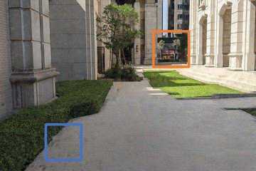
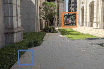
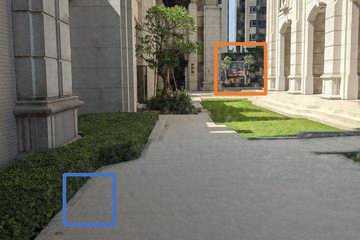
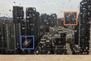
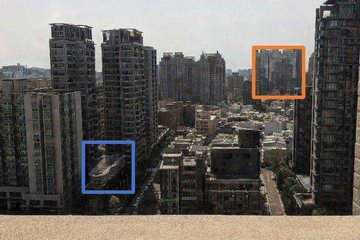
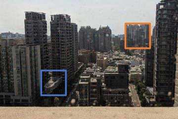
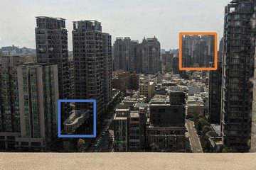
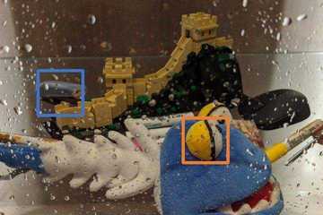
We present a learning-based approach for removing unwanted obstructions, such as window reflections, fence occlusions, or adherent raindrops, from a short sequence of images captured by a moving camera. Our method leverages motion differences between the background and obstructing elements to recover both layers. Specifically, we alternate between estimating dense optical flow fields of the two layers and reconstructing each layer from the flow-warped images via a deep convolutional neural network. This learning-based layer reconstruction module facilitates accommodating potential errors in the flow estimation and brittle assumptions, such as brightness consistency. We show that the proposed approach learned from synthetically generated data performs well to real images. Experimental results on numerous challenging scenarios of reflection and fence removal demonstrate the effectiveness of the proposed method.
Index Terms:
reflection removal, fence removal, optical flow, layer decomposition, computational photography.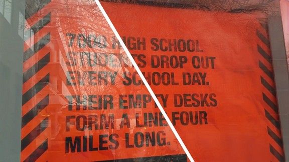
1 Introduction
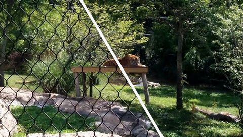
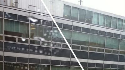
Capturing clean photographs through reflective surfaces (such as windows) or occluding elements (such as fences) is challenging as the captured images inevitably contain both the scenes of interests and the obstructions caused by reflections or occlusions. An effective solution to recover the underlying clean image is thus of great interest for improving the quality of the images captured under such conditions or allowing computers to form a correct physical interpretation of the scene, e.g., enabling a robot to navigate in a scene with windows safely.
Recent efforts have been focused on removing unwanted reflections or occlusions from a single image [1, 2, 3, 4, 5, 6, 7, 8]. These methods either leverage the ghosting cues [9] or adopt learning-based approaches to capture the prior of natural images [2, 3, 6, 7, 8]. While significant advances have been shown, separating the clean background from reflection/occlusions is fundamentally ill-posed and often requires a high-level semantic understanding of the scene. In particular, the performance of learning-based methods often degrades significantly for out-of-distribution images.
To tackle these challenges, multi-frame approaches exploit the fact that the background scene and the occluding elements are located at different depths with respect to the camera (e.g., virtual depth of window reflections). Consequently, taking multiple images from a slightly moving camera reveals the motion differences between the two layers [10, 11, 12, 13, 14, 15]. A number of approaches exploit such visual cues for reflection or fence removal from a video [10, 12, 11, 13, 16, 14, 15, 17, 18, 19]. Xue et al. [20] propose a unified computational framework for obstruction removal and show impressive results on several real input sequences. The formulation, however, requires a computationally expensive optimization process and relies on strict assumptions of brightness constancy and accurate dense motion estimation. To alleviate these issues, recent work [19] explores model-free methods by learning a generic 3D convolutional neural network (CNN). Nevertheless, the CNN-based methods do not produce results with comparable quality as optimization-based algorithms on real input sequences.
In this work, we propose a multi-frame obstruction removal algorithm that exploits the strength of both optimization-based and learning-based methods. Inspired by the optimization-based approaches [17, 20], our algorithm alternates between the dense motion estimation and background/obstruction layer reconstruction steps in a coarse-to-fine manner. Our framework builds upon the optimization-based formulation of [17, 20] but differs in that our model is purely data-driven and does not rely on classical assumptions such as brightness constancy [17, 20], accurate flow fields [14], or planar surface [15] in the scene. When these assumptions do not hold (e.g., occlusion/dis-occlusion, motion blur, inaccurate flow), classical approaches may fail to reconstruct clear foreground and background layers.
On the other hand, data-driven approaches learn from diverse training data and can tolerate errors when these assumptions are violated. The explicit modeling of dense motion within each layer facilitates us to progressively recover detailed content in the respective layers. Instead of relying on hand-crafted objectives for recovering these layers, we use the learning-based method for fusing flow-warped images to accommodate potential violations of brightness constancy and errors in flow estimation. We train our fusion network using a synthetically generated dataset and demonstrate that it performs well to unseen real-world sequences. In addition, we present an online optimization process to further improve the visual quality of particular testing sequences. We show that the proposed method performs favorably against existing learning-based and optimization-based algorithms on a wide variety of challenging sequences and applications.
The preliminary version of this work has been published in CVPR 2020 [21]. In this paper, we further improve our method in three key aspects.
-
1.
We present an improved layer reconstruction model that allows us to take an arbitrary number of input frames.
-
2.
We apply meta-learning to facilitate the efficient adaptation of our pre-trained model to a particular testing sequence. Our results show improvement for both the runtime speed and visual quality.
-
3.
We incorporate a realistic reflection image synthesis model [8] and extend it with a variety of data augmentation to generate more realistic and diverse training sequences.
We show extensive experimental results to validate our design choices. Experiments show that our improved method significantly outperforms our CVPR work on both quantitative and qualitative evaluations.
The main contributions of this work are:
-
1.
We integrate the optimization-based formulation into a learning-based method for robustly separating background/obstruction layers. Meta-learning is employed to reduce the runtime.
-
2.
We present a transfer learning strategy that first pre-trains the model using synthetic data and then fine-tunes on real sequence with an unsupervised optimization objective function to achieve state-of-the-art performance in the context of obstruction removal.
-
3.
We show our model can be easily extended to handle other types of obstruction removal problems, e.g., fence and adherent raindrop removal.
2 Related Work
Multi-frame reflection removal. Existing methods often exploit the differences of motion patterns between the background and reflection layers [15, 20], and impose natural image priors [22, 15, 20]. These methods differ in modeling the motion fields, e.g., SIFT flow [14], homography [15], and dense optical flow [20]. Recent advances include optimizing temporal coherence [17] and learning-based layer decomposition [19] for reflection removal. In contrast to the scheme based on a generic spatio-temporal CNN [19], our method explicitly models the dense flow fields of the background and obstruction layers to obtain cleaner results on real sequences.
Single-image reflection removal.
A number of approaches have been proposed to remove unwanted reflections with only one single image as input. Existing methods exploit various cues, including ghosting effect [9], blurriness caused by depth-of-field [23, 24], image priors (either hand-designed [1] or learned from data [7, 8]), and the defocus-disparity cues from dual pixel sensors [25]. Despite the demonstrated success, reflection removal from a single image remains challenging due to the nature of this highly ill-posed problem and the lack of motion cues. Our work instead utilizes the motion cues from image sequences captured with a slightly moving camera for separating the background and reflection layers.
Occlusion and fence removal.
Occlusion removal aims to eliminate the captured obstructions, e.g., fence or adherent raindrops on an image or sequences, and provide a clear view of the scene. Existing methods detect fence patterns by exploiting visual parallax [26], dense flow field [20], disparity maps [27], or using graph-cut [28]. One recent work leverages a CNN for fence segmentation [18] and recovers the occluded pixels using optical flow. Our method also learns deep CNNs for optical flow estimation and background image reconstruction. Instead of focusing on fence removal, our formulation is more general and applicable to different obstruction removal tasks.
Layer decomposition.
Image layer decomposition is a long-standing problem in computer vision, e.g., intrinsic image [29, 30], depth, normal estimation [31, 32], relighting [33, 34], and inverse rendering [35, 36]. Our method is inspired by the development of these layer decomposition approaches, particularly in the ways of leveraging both the physical image formation constraints and data-driven priors.
Video completion Video completion aims to fill in plausible content in missing regions of a video [37], with applications ranging from object removal, full-frame video stabilization, and watermark/transcript removal. State-of-the-art methods estimate the flow fields in both known and missing regions to constrain the content synthesis [38, 39, 40], and generate temporally coherent completion. The obstruction removal problem resembles a video completion task. However, the crucial difference is that no manual mask selection is required for removing the fences/obstructions from videos.
Online optimization (training on testing data) Learning from the test data has been an effective way to reduce the domain discrepancy between the training/testing distributions. Examples abound, including using geometric constraints [41, 42], self-supervised losses [43], deep image priors [44, 45, 46], and online template update [47]. Similar to these methods, we fine-tune our background/obstruction reconstruction network on a particular test sequence to further improve the separation. Our unsupervised loss directly measures how well the recovered background/obstruction and the dense flow fields explain all the input frames.
Meta-learning. Meta-learning refers to a class of algorithms that aim to learn a “learner" which can quickly adapt to a new task with few training examples. Existing meta-learning algorithms can be categorized as black-box adaptation [48, 49], metric-based [50, 51, 52, 53], and optimization-based methods [54, 55]. Our work applies an optimization-based meta-learning algorithm [54, 55, 56] for learning a weight initialization that can adapt to a new task with few gradient updates from a small number of training examples. Specifically, we apply Reptile [55] to improve the model adaptation to the testing sequence.
3 Proposed Algorithm
Given a sequence of frames, our goal is to decompose each frame into two layers, one for the target (clean) background and the other for the obstruction caused by reflection/fence/raindrops. Decomposing an image sequence into background and obstruction is difficult as it involves solving two tightly coupled problems: motion decomposition and layer reconstruction. Without an accurate motion decomposition, the layers cannot be reconstructed faithfully due to the misalignment from inaccurate motion estimation (e.g., optical flow). On the other hand, without well-reconstructed background and obstruction layers, the motion cannot be accurately estimated because of the mixed contents. Due to the nature of this chicken-and-egg problem, there is no ground to start with because we do not have information for both motion and layer content.
3.1 Algorithmic overview
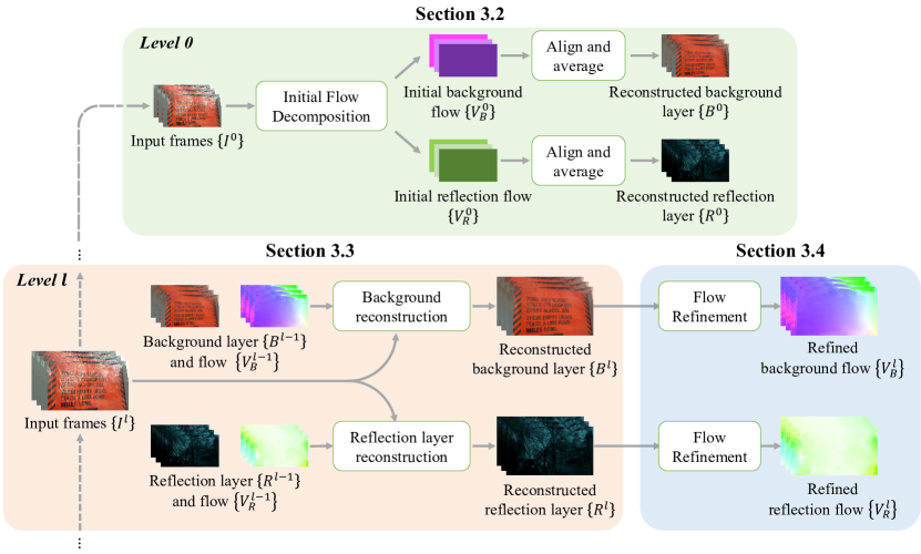
In this work, we propose to learn deep CNNs to tackle the above-mentioned challenges. Our proposed method mainly consists of three modules: 1) initial flow decomposition, 2) background and obstruction layer reconstruction, and 3) optical flow refinement. Our method takes frames as input and decomposes the keyframe frame into a background layer and reflection layer at a time. We reconstruct the output images in a coarse-to-fine manner within an -level hierarchy. First, we estimate the flows at the coarsest level from the initial flow decomposition module (Section 3.2). Next, we progressively reconstruct the background/obstruction layers (Section 3.3) and refine optical flows (Section 3.4) until the finest level. Figure 2 shows an overview of our method. Our framework can be applied to several layer decomposition problems, such as reflection/obstruction/fence/rain removal. Without loss of generality, we use the reflection removal task as an example to introduce our algorithm. We describe the details of the three modules in the following sections.
3.2 Initial flow decomposition
We first predict optical flows for both the background and reflection layers at the coarsest level (), which is the essential starting point of our algorithm. Instead of estimating dense flow fields, we propose to learn a uniform motion vector for each layer. Our initial flow decomposition network consists of two sub-modules: 1) a feature extractor, and 2) a layer flow estimator. The feature extractor first generates feature maps for all the input frames at a spatial resolution. We then construct a cost volume between frame and frame via a correlation layer [57]:
| (1) |
where and are the extracted features of frame and , respectively, and indicates the pixel index. Since the spatial resolution is quite small at this level, we set the correlation layer’s search range to only 4 pixels. The cost volume is then concatenated with the feature and fed into the layer flow estimator.
The layer flow estimator uses the global average pooling and fully-connected layers to generate two global motion vectors. Next, we tile the global motion vectors into two uniform flow fields (at a spatial resolution): for the background layer and for the reflection layer. We provide the detailed architecture of our initial flow decomposition module in the supplementary material.

3.3 Background/Reflection layer reconstruction
The layer reconstruction module aims to reconstruct a clean background image and a reflection image . Although the goals of these two tasks are similar in spirit, the characteristics of the background and reflection layers are essentially different. For example, the background layers are often more dominant in appearance but could be occluded in some frames. On the other hand, the reflection layers are often blurry and darker. Consequently, we train two independent networks for reconstructing the background and reflection layers. These two models have the same architecture but do not share the network parameters. In the following, we only describe the details for background layer reconstruction; the reflection layer is reconstructed in a similar fashion.
We reconstruct the background layer in a coarse-to-fine fashion. At the coarsest level (), we first use the flow fields estimated from the initial flow decomposition module to align the neighboring frames. Then, we compute the average of all the background-registered frames as the predicted background image:
| (2) |
where is the downsampled frame , and is the warping operation with bilinear sampling.
At the -th level, the network takes as input the reconstructed background image , reflection image , background optical flows from the previous level as well as the input frames at the current level. To reconstruct the background image of the keyframe at the current level, the background reconstruction module consists of three steps: 1) frame registration, 2) feature extraction, and 3) image reconstruction.
Frame registration. We first upsample the background flow fields by and align all the input frames to the keyframe :
| (3) |
where denotes the bilinear upsampling operator.
Feature extraction. For each non-keyframe image , we first concatenate the following five features into a group:
-
1.
background-registered frame ,
-
2.
difference map ,
-
3.
visibility mask ,
-
4.
upsampled background , and
-
5.
upsampled reflection layers .
The visibility mask is computed by warping the grid coordinates with the flow and checking whether each pixel stays within the image boundary.
For input frames, we can construct groups. We then apply 5 convolutional layers to extract features from each group:
| (4) |
where is the feature extraction network. We use a max pooling layer to collapse these groups of features into one representative feature. Note that the weights in are shared among all the groups. By using the weight sharing and max pooling, our layer reconstruction module is capable of processing arbitrary numbers of input frames.
Image reconstruction. Our background reconstruction network takes the collapsed feature as input and learns to predict the residual map of the background keyframe. The background frame is reconstructed by:
| (5) |
where is the background reconstruction network.
Note that the reflection layer is also involved in the reconstruction of the background layer, which couples the background and reflection reconstruction networks together for joint training. Figure 3 illustrates an overview of the background reconstruction network at the -th level.
3.4 Optical flow refinement
After reconstructing all the background images at level , we then refine the background optical flows. We use the pre-trained PWC-Net [57] to estimate the flow fields between a paired of background images:
| (6) |
where PWC denotes the pre-trained PWC-Net. Note that the PWC-Net is fixed and not updated with the other sub-modules of our model during the training stage.
3.5 Network training
To improve training stability, we employ a two-stage training procedure. At the first stage, we train the initial flow decomposition network with the following loss:
| (7) |
where is the bilinear downsampling operator, and denote the ground-truth background and reflection layers, respectively. We use the pre-trained PWC-Net to compute optical flows and downsample the flows by as the pseudo ground-truth flows to train the initial flow decomposition network.
Next, we freeze the initial flow decomposition network and train the layer reconstruction networks with an image reconstruction loss:
| (8) |
and a gradient loss:
| (9) |
where is the spatial gradient operator. The gradient loss encourages the network to reconstruct faithful edges to further improve visual quality. The overall loss for training the layer reconstruction networks is:
| (10) |
where the weight is empirically set to 1 in all our experiments. We train both the initial flow decomposition and layer reconstruction networks with the Adam optimizer [58] with a batch size of 2. We set the learning rate to for the first 100K iterations and then decrease to for another 100K iterations. The number of pyramid levels is set to 5. We describe the training steps of our two-stage training strategy Algorithm 1.
3.6 Meta-learning for fast adaptation
To ensure that our model can be adapted to handle real data more effectively and efficiently, we apply a meta-learning technique to finetune our pre-trained model with both the synthetic and real sequences. Specifically, we use the first-order meta-learning algorithm [59] and describe our meta training step in Algorithm 2. When a training batch is sampled from synthetic data, we minimize the supervised loss (10). On the other hand, when a training batch is sampled from real data, we optimize a warping consistency loss:
| (11) |
where is the reconstructed input frame from the warped background and reflection layers. The warping consistency loss enhances fidelity by enforcing that the predicted background and reflection layers should be warped back and composited into the original input frames. In addition, we also incorporate the total variation loss:
| (12) |
which encourages the network to generate natural images by following the sparse gradient image prior. The overall unsupervised loss for training on real data is defined as:
| (13) |
where the weight is empirically set to 0.1 in all our experiments. The update parameter is set to in our experiment. We show in Section 4.2 that the meta-learning is able to speed up the online optimization as well as improve the reconstruction performance.
3.7 Online optimization
We adopt an online refinement method to fine-tune our pre-trained model with a real test sequence by optimizing the unsupervised loss in (13). Note that we freeze the weights of the PWC-Net and only update the background/reflection layer reconstruction modules in both the meta-learning and online optimization stages. We fine-tune our model on every single input sequence for 200 iterations. The fine-tuning step takes about 3 minutes for a sequence with a 1296 864 spatial resolution. We describe the training steps of our unsupervised online optimization in Algorithm 3.
3.8 Extension to other obstruction removal tasks
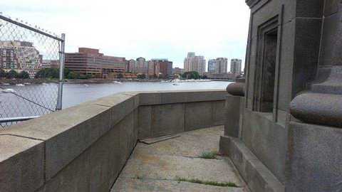
Our proposed framework can be easily extended to handle other obstruction removal tasks, such as fence and adherent raindrop removal. First, we remove the reflection layer reconstruction module and only predict the background layers. Second, the background image reconstruction network outputs an additional channel as the alpha map for segmenting the obstruction layer. We do not estimate flow fields for the obstruction layer as the flow estimation network cannot handle the repetitive structures (e.g., fence) or tiny objects (e.g., raindrops) well and often predicts noisy results. With such a design change, our model is able to perform well on the fence and adherent raindrop removal tasks. We use the fence segmentation dataset [18] and alpha matting dataset [60] to generate training data for both tasks. Fig. 4 gives an overview of adapting our framework to the fence removal task.
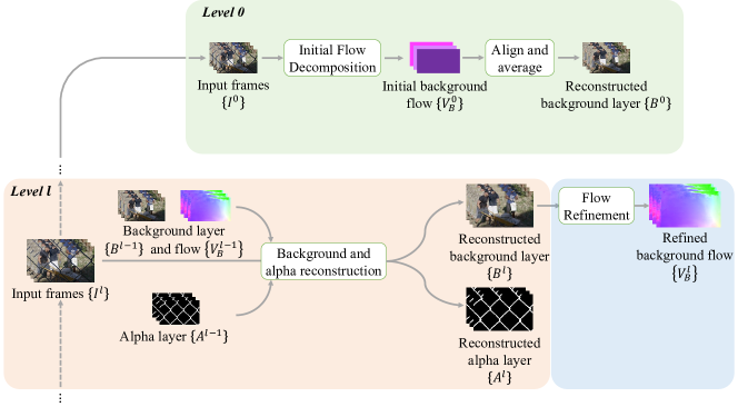
To apply our online optimization for obstruction removal, we first extract the foreground layer by , where denotes the predicted alpha map. Then, we compute the foreground flow with the pre-trained PWC-Net. The reconstructed frame can be approximated by:
| (14) |
We replace in (11) as the warping consistency loss used in the meta-learning and online optimization stages for fence removal.
3.9 Synthetic sequence generation
Since it is difficult to collect real sequences with ground-truth reflection and background layers, we use the Vimeo-90k dataset [61] to generate synthetic sequences for training. Out of the 91,701 sequences in the Vimeo-90k training set, we randomly select two sequences as the background and reflection layers. In our preliminary work [21], we adopt the following three steps to generate a synthetic sequence. First, we warp the sequences using random homography transformations. We then randomly crop the sequences to a spatial resolution of pixels. The composition is applied frame by frame using the realistic reflection image synthesis model proposed by previous work [2, 8].
In this work, we improve the data synthesis pipeline in [21] to generate more diverse training data. During the training stage, we apply on-the-fly random color augmentation, including hue, saturation, brightness, and contrast, on both background and reflection layers. As suggested by previous work [2, 8], to simulate the effect that the reflection layer is usually out-of-focus, we apply a Gaussian filter on the reflection layer with kernel size randomly selected from [3, 17] and standard deviation randomly sampled from [0.8, 2.9].
After blending the background and reflection layers, we apply Gaussian noise with standard deviation randomly selected from and JPEG compression artifacts with compression quality randomly selected from . In addition, for simulating vignetting, we add a Gaussian falloff with a randomly selected kernel size to the synthetic image. As our model is able to tackle arbitrary input frames, we randomly sample 2 to 7 input frames at each training iteration. We also provide examples of the training pairs generated from our pipeline in the supplementary materials.
4 Experimental Results
| Stone | 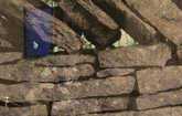 |
 |
 |
| Toy | 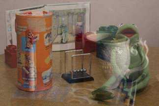 |
 |
 |
| Hanoi |  |
 |
 |
| Input (keyframe) | Recovered background | Recovered obstruction |
| Method | Stone | Toy | Hanoi | |||||||||||||||
| Background | Reflection | Background | Reflection | Background | Obstruction | |||||||||||||
| SSIM | NCC | LMSE | SSIM | NCC | LMSE | SSIM | NCC | LMSE | SSIM | NCC | LMSE | SSIM | NCC | LMSE | SSIM | NCC | LMSE | |
| Li and Brown [14] | 0.7993 | 0.9334 | 0.0114 | 0.2038 | 0.3668 | 0.0134 | 0.6877 | 0.7068 | 0.0196 | 0.1092 | 0.6607 | 0.0105 | - | - | - | - | - | - |
| Guo et al. [15] | 0.5292 | 0.7251 | 0.0571 | 0.4749 | 0.1006 | 0.2664 | 0.7081 | 0.7215 | 0.0231 | 0.4892 | 0.6625 | 0.0983 | - | - | - | - | - | - |
| Xue et al. [20] | - | 0.9738 | - | - | 0.8433 | - | - | 0.8985 | - | - | 0.7536 | - | - | 0.9921 | - | - | 0.7079 | - |
| Alayrac et al. [19] | 0.7942 | 0.9351 | 0.0092 | 0.7633 | 0.1641 | 0.0407 | 0.7569 | 0.7972 | 0.0088 | 0.3652 | 0.5260 | 0.0152 | - | - | - | - | - | - |
| Liu et al. [21] | 0.8598 | 0.9632 | 0.0052 | 0.2041 | 0.7002 | 0.0277 | 0.7696 | 0.9477 | 0.0053 | 0.5342 | 0.8696 | 0.0100 | 0.9238 | 0.9929 | 0.0018 | 0.2991 | 0.5621 | 0.2034 |
| Ours | 0.8635 | 0.9315 | 0.0062 | 0.5146 | 0.3018 | 0.0268 | 0.8494 | 0.9542 | 0.0048 | 0.3371 | 0.9046 | 0.0056 | 0.9457 | 0.9938 | 0.0018 | 0.3115 | 0.8549 | 0.1583 |
In this section, we present visual and quantitative comparisons with the state-of-the-art obstruction removal algorithms as well as provide detailed ablation study justifying the design choices our method. Complete visual results can be found at https://alex04072000.github.io/SOLD/. We also provide the source code and pre-trained models at https://github.com/alex04072000/SOLD.
4.1 Comparisons with State-of-the-arts
Controlled sequences.
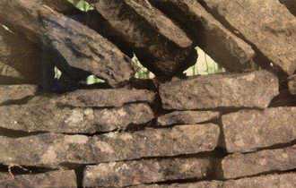
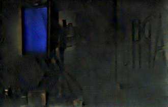
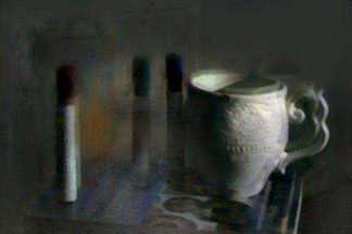
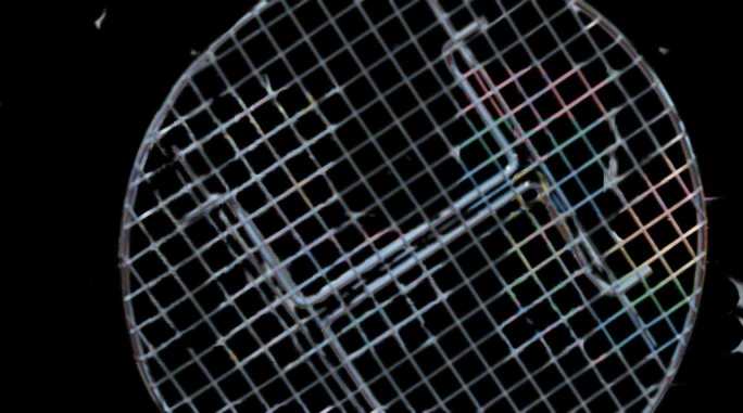
We first evaluate on the controlled sequences provided by Xue et al. [20], which contain three videos with ground-truth background and reflection layers. We evaluate the proposed method with the approaches by Li and Brown [14], Guo et al. [15], Xue et al. [20], and Alayrac et al. [19] and report the SSIM, normalized cross-correlation (NCC) scores [62, 20], and LMSE [63] in TABLE I. SSIM measures the structural similarity between the recovered and ground-truth images. NCC measures the overall quality while ignoring the global scaling of the intensity since the ground-truth images are only defined up to a scaling factor. LMSE is also a scale-invariant metric but often used to measure errors locally. They are not always consistent since they are designed to compare images from different aspects and characteristics. Fig. 5 shows our method performs favorably against other approaches in reconstructing background and reflection/obstruction layers.
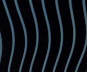
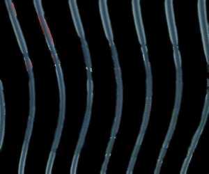
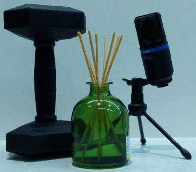
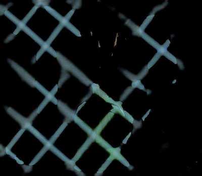
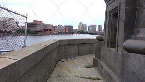
Other than the three sequences provided by Xue et al. [20], to the best of our knowledge, there are no other publicly available sequences with obstruction having ground truths. In light of this, we collect six sequences with ground truth. Specifically, we put a camera on a tripod to capture the background scenes behind the obstructions (e.g., glasses or fences). The captured images, therefore, contain the background objects and the obstructions (reflections or obstacles). We then lace a black flannel behind the obstruction to occlude the background for capturing the ground-truth obstruction images. Finally, we remove the obstruction to capture the ground-truth images of the background scenes. We repeat the process for five different camera positions. Our dataset contains six scenes: two with reflection, two with a fence, and two with semi-transparency. For the scenes with semi-transparency, we cannot obtain the ground-truth obstruction images. The reason is, after we occlude the background with a black flannel, the captured image becomes extremely dark as there is no light from behind. Thus, we only provide ground-truth background images for the scenes with semi-transparency. We conduct quantitative comparisons with other methods with these six sequences, and TABLE II shows the results. Note that Li and Brown [14] and Guo et al. [15] are not methods designed for removing fences and semi-transparent objects. We still include the results as references. Our method significantly outperforms the compared methods, including the preliminary version of this work [21]. Fig. 6 displays the dataset and visual results of our method.
| Method | Reflection 1 | Reflection 2 | Fence 1 | |||||||||||||||
| Background | Reflection | Background | Reflection | Background | Obstruction | |||||||||||||
| SSIM | NCC | LMSE | SSIM | NCC | LMSE | SSIM | NCC | LMSE | SSIM | NCC | LMSE | SSIM | NCC | LMSE | SSIM | NCC | LMSE | |
| Li and Brown [14] | 0.7829 | 0.9259 | 0.0177 | 0.3546 | 0.3971 | 0.0148 | 0.5746 | 0.6991 | 0.0846 | 0.3064 | 0.0822 | 0.0187 | 0.6576 | 0.7571 | 0.0406 | 0.0964 | 0.0134 | 0.2921 |
| Guo et al.[15] | 0.6034 | 0.6690 | 0.0702 | 0.3279 | 0.1013 | 0.2005 | 0.6213 | 0.6784 | 0.0694 | 0.3288 | 0.0073 | 0.2953 | 0.6227 | 0.8791 | 0.0275 | 0.2088 | -0.1744 | 0.5705 |
| Alayrac et al.[19] | 0.8304 | 0.9641 | 0.0085 | 0.6884 | 0.0630 | 0.0540 | 0.7947 | 0.9287 | 0.0161 | 0.6060 | -0.1024 | 0.0876 | 0.7478 | 0.9106 | 0.0311 | 0.3593 | 0.0822 | 0.3448 |
| Liu et al.[61] | 0.8852 | 0.9788 | 0.0054 | 0.3475 | 0.4181 | 0.2371 | 0.8543 | 0.9674 | 0.0065 | 0.3425 | 0.2245 | 0.1486 | 0.9519 | 0.9956 | 0.0017 | 0.3698 | 0.9170 | 0.0797 |
| Ours | 0.9167 | 0.9867 | 0.0036 | 0.4839 | 0.4968 | 0.0412 | 0.8939 | 0.9826 | 0.0069 | 0.3639 | 0.5265 | 0.0396 | 0.9711 | 0.9975 | 0.0010 | 0.3530 | 0.8932 | 0.0994 |
| Method | Fence 2 | Semi-transparency | Adherent raindrop | |||||||||||||||
| Background | Reflection | Background | Reflection | Background | Obstruction | |||||||||||||
| SSIM | NCC | LMSE | SSIM | NCC | LMSE | SSIM | NCC | LMSE | SSIM | NCC | LMSE | SSIM | NCC | LMSE | SSIM | NCC | LMSE | |
| Li and Brown [14] | 0.7458 | 0.9162 | 0.0116 | 0.2102 | 0.4125 | 0.1109 | 0.7694 | 0.8618 | 0.0272 | - | - | - | 0.8102 | 0.8584 | 0.0095 | - | - | - |
| Guo et al.[15] | 0.7536 | 0.9339 | 0.0228 | 0.4345 | 0.4920 | 0.1059 | 0.6630 | 0.6953 | 0.0649 | - | - | - | 0.7375 | 0.7958 | 0.0255 | - | - | - |
| Alayrac et al.[19] | 0.8003 | 0.9754 | 0.0069 | 0.4816 | 0.3996 | 0.1946 | 0.8073 | 0.8880 | 0.0213 | - | - | - | 0.8043 | 0.8514 | 0.0119 | - | - | - |
| Liu et al.[61] | 0.9118 | 0.9904 | 0.0038 | 0.3658 | 0.6800 | 0.3509 | 0.9009 | 0.9832 | 0.0078 | - | - | - | 0.9031 | 0.9763 | 0.0034 | - | - | - |
| Ours | 0.9416 | 0.9941 | 0.0025 | 0.3392 | 0.6865 | 0.3619 | 0.9378 | 0.9903 | 0.0047 | - | - | - | 0.9312 | 0.9869 | 0.0019 | - | - | - |
| Reflection 1 |  |
 |
 |
 |
 |
| Reflection 2 |  |
 |
 |
 |
 |
| Fence 1 |  |
 |
 |
 |
 |
| Fence 2 | 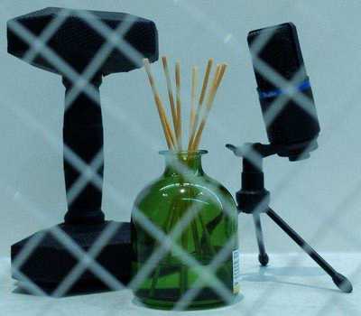 |
 |
 |
 |
 |
| Semi-transparency |  |
 |
 |
 |
|
| Adherent raindrop |  |
 |
 |
 |
|
| Input (keyframe) | Background GT | Obstruction GT | Recovered background | Recovered obstruction |
Synthetic sequences.
We synthesize 100 sequences from the Vimeo-90k test set using the method described in Section 3.9. We evaluate our approach with five single-image reflection removal methods [2, 3, 6, 7, 8], and three multi-frame approaches [19, 15, 14]. We use the default parameters of each method to generate the results. Since the source code or pre-trained models of Alayrac et al. [19] are not available, we re-implement their model and train on our training dataset (with the help from the authors). Note that our reimplementation results for Alayrac et al. [19] are not as good as those presented in their paper. The reason is that we train their method using our data generation scheme for fair comparison while their model was trained on a much large dataset containing 400k 250-frame videos. It shows, thanks to having more inductive bias, our method does not require a large training dataset of long sequences compared to their method. TABLE III shows the average PSNR, SSIM [64], NCC, and LMSE [63] metrics. Note that the proposed method without the online optimization already performs favorably against existing approaches. By incorporating the online optimization, we can further improve the average SSIM and NCC on both the background and reflection layers.
| Method | Background | Reflection | ||||||||
| PSNR | SSIM | NCC | LMSE | PSNR | SSIM | NCC | LMSE | |||
| Single image | CEILNet [2] | CNN-based | 18.64 | 0.6808 | 0.8102 | 0.0408 | - | - | - | - |
| Zhang et al. [8] | CNN-based | 17.27 | 0.6861 | 0.8142 | 0.0272 | 15.61 | 0.4271 | 0.5368 | 0.1173 | |
| BDN [7] | CNN-based | 15.49 | 0.6654 | 0.7076 | 0.0426 | - | - | - | - | |
| ERRNet [6] | CNN-based | 20.19 | 0.7530 | 0.8157 | 0.0198 | - | - | - | - | |
| Jin et al. [3] | CNN-based | 16.78 | 0.6993 | 0.7321 | 0.0242 | 9.13 | 0.3069 | 0.3779 | 0.1276 | |
| Multiple images | Li and Brown [14] | Optimization-based | 15.36 | 0.5950 | 0.6155 | 0.0802 | 7.00 | 0.2047 | 0.2809 | 0.1335 |
| Guo et al. [15] | Optimization-based | 13.51 | 0.4835 | 0.5460 | 0.0909 | 11.85 | 0.2408 | 0.2517 | 0.1975 | |
| Alayrac et al. [19] | CNN-based | 21.12 | 0.7277 | 0.8520 | 0.0248 | 16.84 | 0.5283 | 0.6225 | 0.1706 | |
| Liu et al. [21] | CNN-based | 23.82 | 0.8082 | 0.8936 | 0.0150 | 17.65 | 0.5338 | 0.6299 | 0.1103 | |
| Ours w/o online optimization | CNN-based | 26.75 | 0.8742 | 0.9247 | 0.0114 | 20.40 | 0.6329 | 0.7731 | 0.0974 | |
| Ours | CNN-based | 25.98 | 0.8916 | 0.9516 | 0.0169 | 19.81 | 0.7141 | 0.7894 | 0.0921 | |
 |
Background |  |
 |
 |
 |
 |
| Reflection |  |
 |
 |
 |
 |
|
 |
Background |  |
 |
 |
 |
 |
| Reflection |  |
 |
 |
 |
 |
|
 |
Background |  |
 |
 |
 |
 |
| Reflection | 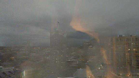 |
 |
 |
 |
 |
|
 |
Background | 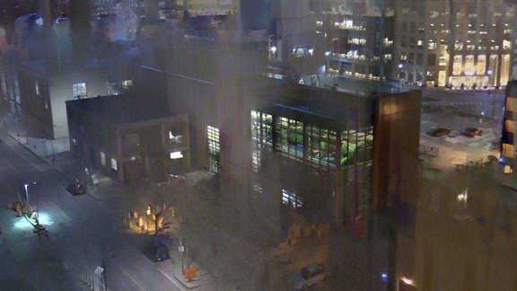 |
 |
 |
 |
 |
| Reflection | 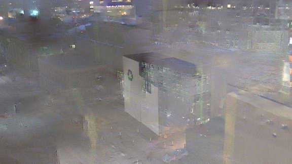 |
 |
 |
 |
 |
|
| Representative input frame | Li and Brown [14] | Xue et al. [20] | Alayrac et al. [19] | Liu et al. [21] | Ours |
 |
Background |  |
 |
 |
 |
 |
| Reflection | 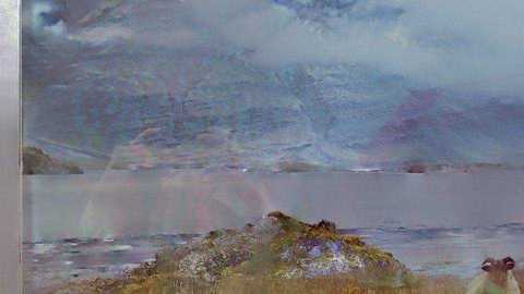 |
 |
 |
 |
 |
|
 |
Background |  |
 |
 |
 |
 |
| Reflection | 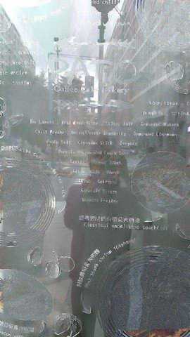 |
 |
 |
 |
 |
|
| Representative input frame | Li and Brown [14] | Guo et al. [15] | Alayrac et al. [19] | Liu et al. [21] | Ours |
 |
Background |  |
 |
 |
 |
| Representative input frame | Reflection | 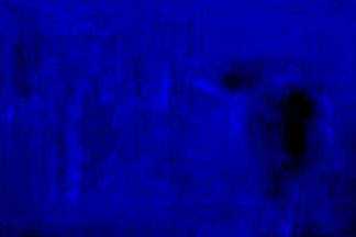 |
 |
 |
 |
 |
Background | 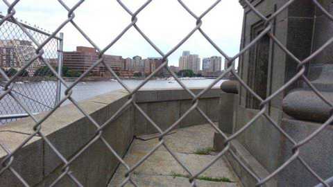 |
 |
 |
 |
| Representative input frame | Alpha |  |
 |
 |
 |
| Pre-training | |||||
| Online optimization | |||||
| Meta-learning |
 |
 |
||
 |
 |
 |
 |
| Input | Xue et al. [20] | ||
 |
 |
||
 |
 |
 |
 |
| Liu et al. [21] | Ours | ||
Real sequences.
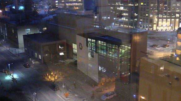
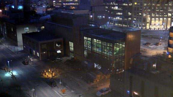
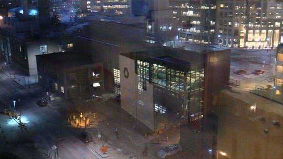
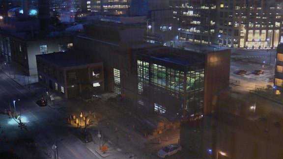
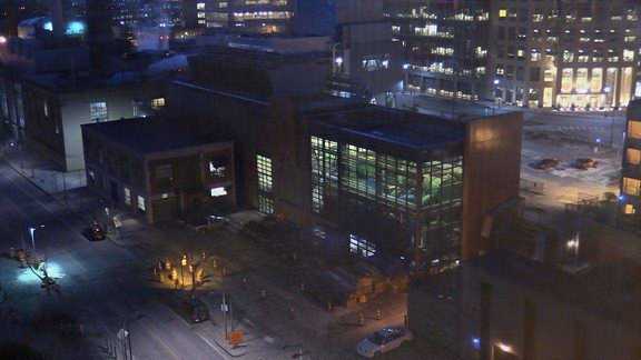
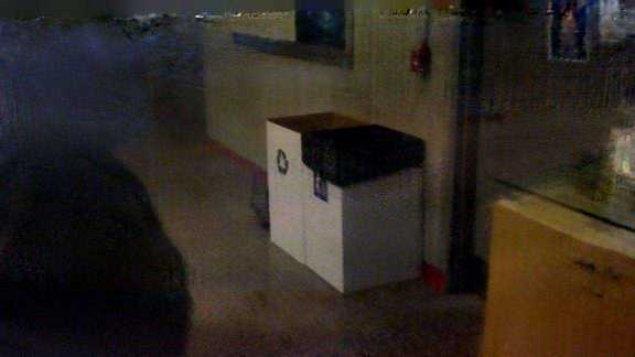
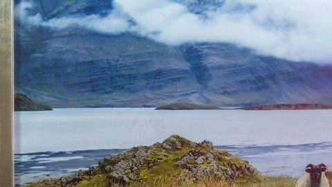
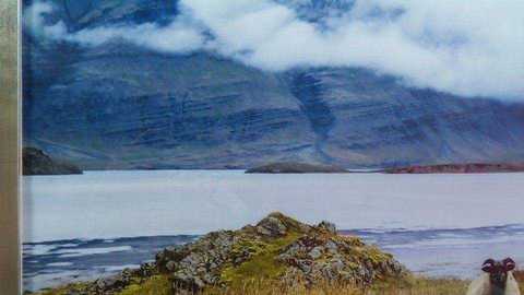
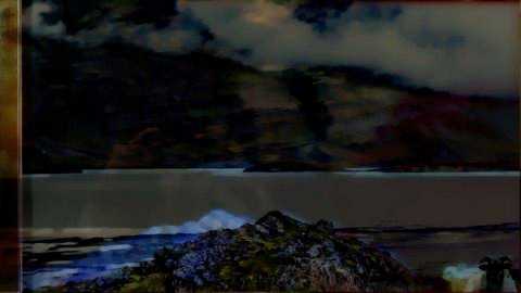
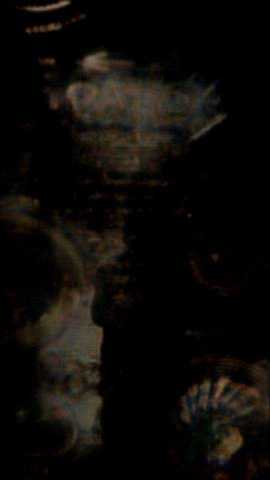
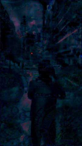
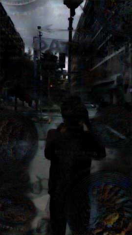
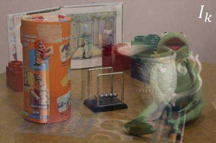
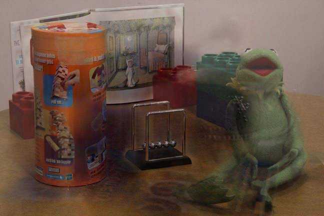
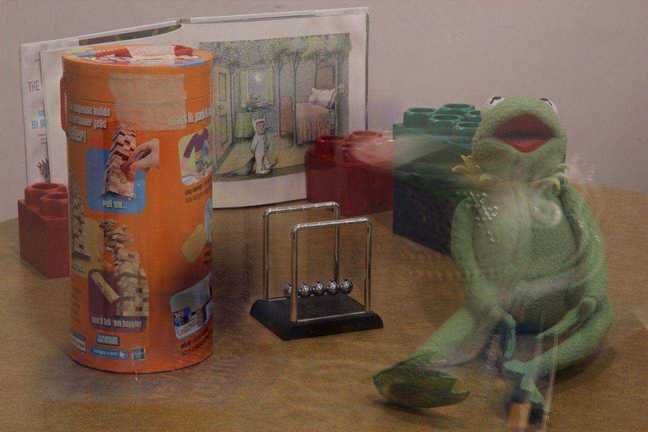
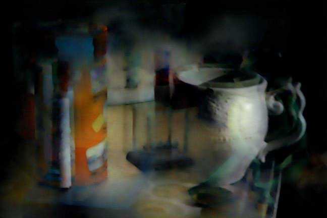
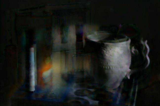
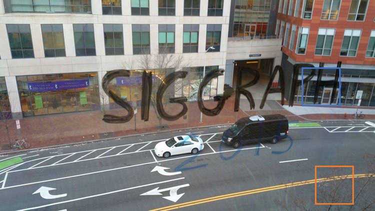
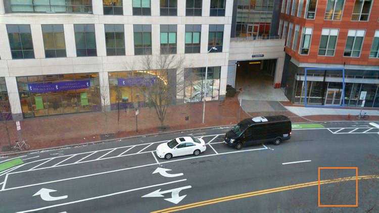
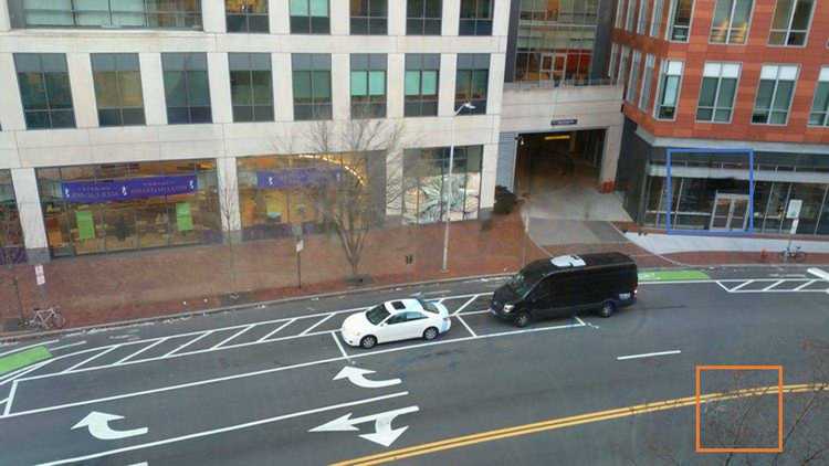
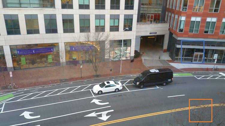
In Fig. 7, we present visual comparisons of real input sequences from [20]. Our method is able to separate the reflection layers better and reconstruct clearer and sharper background images than existing approaches [19, 14, 20, 21]. In addition, we capture another 35 real sequences using iPhone 11 and Google Pixel 3. Some of the sequences contain non-planar background or moving objects in the scenes, which make these sequences particularly challenging. In Fig. 8, we present visual comparisons with [14, 15, 19, 21] on self-captured real input sequences. Fig. 10 shows one example where the inputs contain semi-transparant obstruction such as texts on the glass. Our method can remove the obstruction layer and reconstruct clear background images. Our method can also be applied to remove dense static water drops that attach to the glass. Fig. 11 shows the visual comparisons between our method and a state-of-the-art adherent raindrop removal method DeRaindrop [65]. Our method can better remove the raindrops and maintain details in the recovered background in the scenarios that the method targets for.
| (a) Initial flow decomposition: Predicting uniform flow fields as initialization achieves better results. | (b) Fusion method: Our image reconstruction network recovers better background/reflection than temporal mean/median filtering. | (c) Model training: Both the network pre-training and online optimization are important to the performance of our method. |
| [t] Flow initialization Loss Zero initialization 0.478 Dense flow field 0.236 Uniform flow field (Ours) 0.197 | Image fusion method Loss Temporal mean filtering 0.652 Temporal median filtering 0.555 Image reconstruction network (Ours) 0.197 | Online optimization Pre-training Loss ✓ - 0.468 - ✓ 0.283 ✓ ✓ 0.197 |
4.2 Analysis and Discussions
Initial flow decomposition.
We demonstrate that the uniform flow field initialization plays an important role in our algorithm. We train our model with the following settings: 1) removing the initial flow decomposition network, where the flows at the coarsest level are set to zero, and 2) predicting spatially-varying dense flow fields as the initial flows. TABLE IV(a) reports the validation loss of (10) on our Vimeo-90k validation set, where the model with uniform flow prediction achieves a lower validation loss compared to other alternatives. Initializing the flow fields to zero makes it difficult for the following levels to decompose the background and reflection layers.
| Pyramid level | Validation loss |
| 1 (without coarse-to-fine) | 0.382 |
| 2 | 0.321 |
| 3 | 0.308 |
| 4 | 0.289 |
| 5 | 0.283 |
| 6 | 0.281 |
 |
Background | 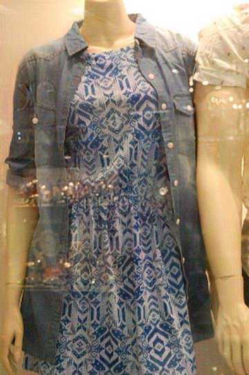 |
 |
 |
 |
Reflection | 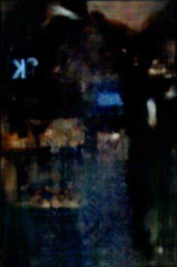 |
 |
 |
| (a) Inputs | (b) Single-scale | (c) 3 scales | (d) 5 scales |

 |
 |
 |
| (a) NCC of the background layer | (b) NCC of the obstruction layer |
 |
 |
| (c) 3 input frames | (d) 5 input frames |
 |
 |
| (e) 7 input frames | (f) 9 input frames |
Image reconstruction network.
To demonstrate the effectiveness of the image reconstruction network, we replace it with a simple temporal filter to fuse the neighbor frames after warping and aligning them with the optical flows. We show in TABLE IV(b) that both the temporal mean and median filters result in large errors (in terms of the validation loss of (10)) as the errors are accumulated across levels.
Online optimization.
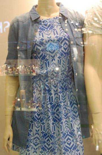
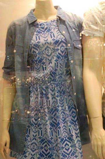
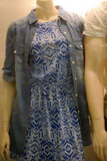
TABLE IV(c) shows that both the network pre-training with synthetic data and online optimization with real data are beneficial to the performance of our model. In Fig. 9, we show that the model without pre-training cannot separate the reflection (or fence) well on the real input sequence. Without online optimization, the background image contains residuals from the reflection layer. After online optimization, our method is able to reconstruct both background and reflection layers well.
Pyramid level.
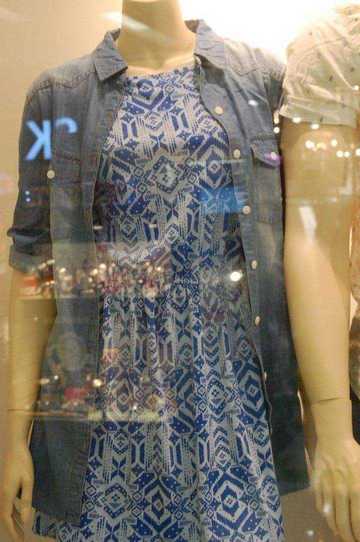
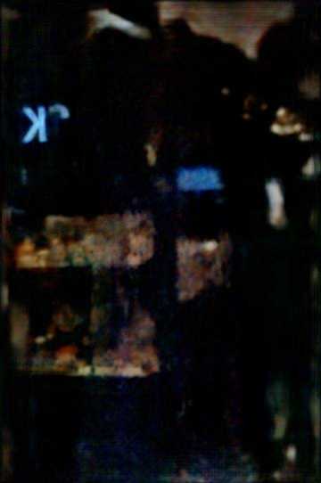
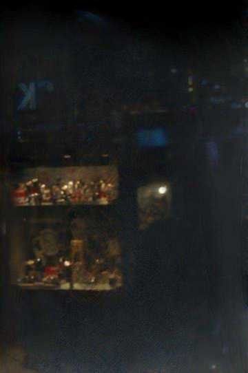
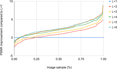
TABLE V shows the ablation study on the number of pyramid levels . Without the coarse-to-fine strategy (), the method gives the worst validation loss. By increasing the pyramid levels, the loss decreases. We choose because (1) the performance nearly saturates after five levels and (2) more levels consume more memory. Fig. 12 compares the visual results of the reconstructed background and reflection with different pyramid levels. With more pyramid levels, our method can reconstruct the background more faithfully. In Fig. 14, we plot the distributions of the validation losses on the 200 images in the validation set. The plot clearly shows that the validation losses distribute more toward the left end (i.e., more images with lower validation losses) when using more pyramid levels. In Fig. 14, we plot the PSNR improvement of the coarse-to-fine (multi-scale) scheme compared to the single-scale baseline. The plot shows that with the pyramid level , about 75% of the images in the validation set have higher PSNR than those with only a single scale. With more pyramid levels, the winning ratio further increases. With the pyramid level , about 50% of the images have more than 2.5dB PSNR improvement compared to the single-scale scheme. About 10% of the images do not gain improvements from the multi-scale scheme with the pyramid level .
| Method | ||
| Data generation used in [21] | 0.9390 | 0.5886 |
| Ours realistic training data generation | 0.9428 | 0.6032 |
Realistic training data generation.
We conduct an experiment to demonstrate the impact of training data generation using controlled sequences Stone and Toy. TABLE VI shows that the NCC scores of reconstructed background and reflection layers are higher by using the proposed realistic training data generation. By training with proposed realistic training data generation, the reconstructed background and reflection layers are much sharper and contain more details.
Number of input frames.
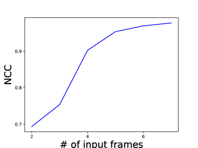
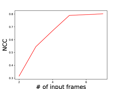
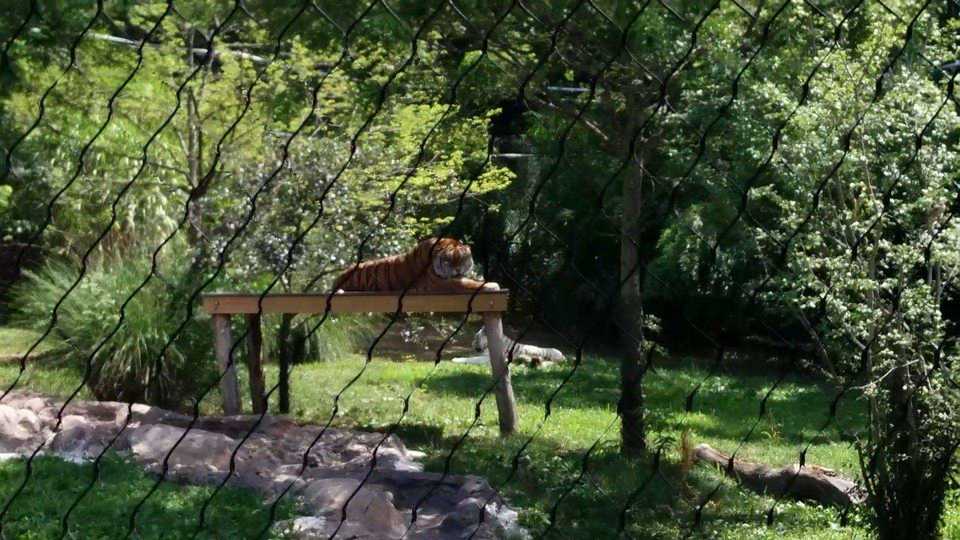
We analyze the effect of the number of input frames on the reconstruction quality using our synthetic sequences. Fig. 15 shows that the results of fence removal are better by giving additional input frames. Fig. 15 also shows that adding additional frames as input leads to improvement in NCC of the reconstructed background and reflection layers.
Input features.
TABLE VII studies the impact of the five input features. Among all the input features, the most important is the registered frames, and the least important is the difference maps. The combination of all five features gives the best performance.
| Registered frame | Difference map | Visibility mask | Upsampled background | Upsampled reflection | Validation loss |
| ✓ | ✓ | ✓ | ✓ | 0.416 | |
| ✓ | ✓ | ✓ | ✓ | 0.288 | |
| ✓ | ✓ | ✓ | ✓ | 0.294 | |
| ✓ | ✓ | ✓ | ✓ | 0.314 | |
| ✓ | ✓ | ✓ | ✓ | 0.322 | |
| ✓ | ✓ | ✓ | ✓ | ✓ | 0.283 |
Meta-learning.
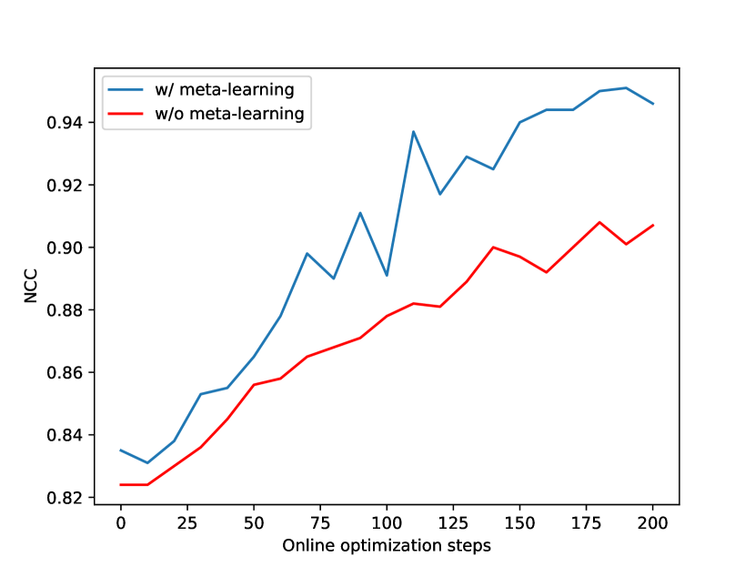
We use the controlled sequence Toy to demonstrate the effectiveness of the meta-learning. Fig. 16 shows that the model pre-trained with meta-learning (blue curve) is able to converge faster and achieve better NCC scores at the same number of online optimization steps. With meta-learning, the number of online optimization steps can be reduced from 1,000 to 200 and achieve similar quality as in [21]. Fig. 9 also demonstrate that the meta-learning can improve the visual quality of the reconstructed background and reflection/fence layers. TABLE VIII shows the comparisons of running time.
| Online optimization | Meta- learning | QVGA () | VGA () | 720p () |
| 1.107 | 2.216 | 9.857 | ||
| 66.056 | 264.227 | 929.182 | ||
| 28.436 | 69.224 | 187.439 |
Running time.
In TABLE IX, we compare the execution time of two optimization-based algorithms [15, 14] and a recent CNN-based method [19] with different input sequences resolutions on a computer with Intel Core i7-8550U CPU and NVIDIA TITAN Xp GPU. Alayrac et al. [19] use a 3D CNN architecture without explicit motion estimation, which results in a faster inference speed. In contrast, our method computes bi-directional optical flows for every pair of input frames in a coarse-to-fine manner, which is slower but achieves much better reconstruction performance.
| Method | QVGA () | VGA () | 720p () |
| Li and Brown [14] | 82.591 | 388.235 | 1304.231 |
| Guo et al. [15] | 64.251 | 369.200 | 1129.125 |
| Alayrac et al. [19] | 0.549 | 2.011 | 6.327 |
| Ours | 28.436 | 69.224 | 187.439 |
Video obstruction removal.
The proposed method takes multiple neighboring frames as input and generates the separation results for a single reference frame at a time. Although predicting each reference frame independently, our method still generates temporally coherent results on the entire video. Here, we compare our method with four video reflection removal approaches [20, 66, 17] and report results in Fig. 17. Both the methods of Xue et al. [20] and Yang et al. [66] take multiple frames as input and generates the middle frame, similar to our model. Xue et al.+ [20] is an extension of [20] which uses the moving window strategy in [66] to improve the temporal consistency. Both Xue et al.++ [20] and Yang et al.++ [66] adopt a temporal average filtering to further reduce the temporal flickering. Nandoriya et al. [17] use a spatiotemporal optimization method to process the entire video sequence jointly.
| NCC | 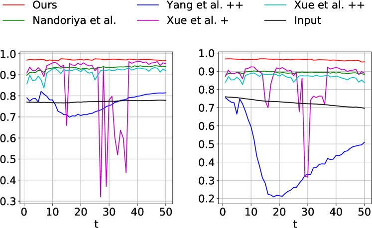 |
|
| SSIM | 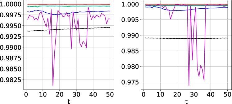 |
|
| Background | Reflection | |
Failure cases.
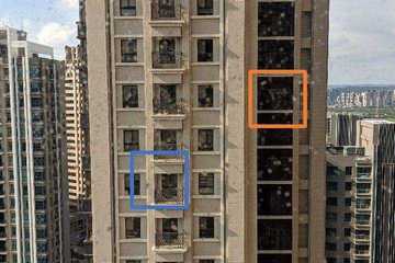
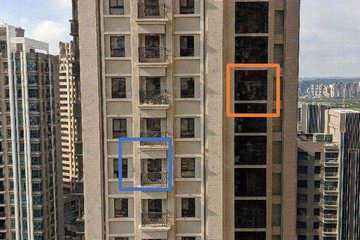
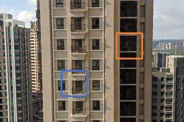
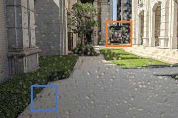
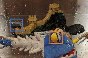
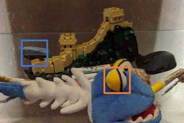
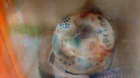
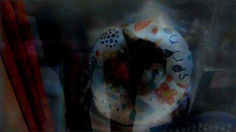
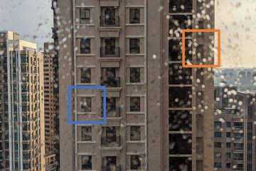
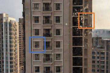
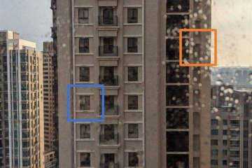
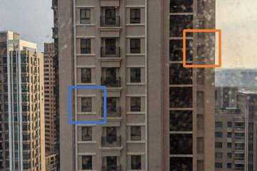
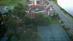
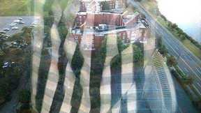
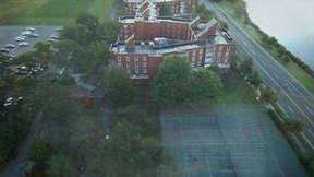
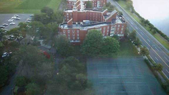
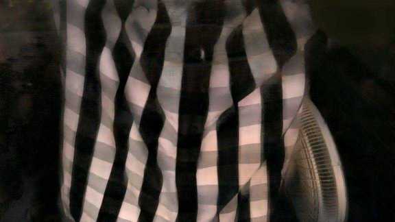
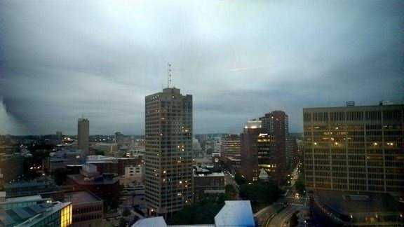
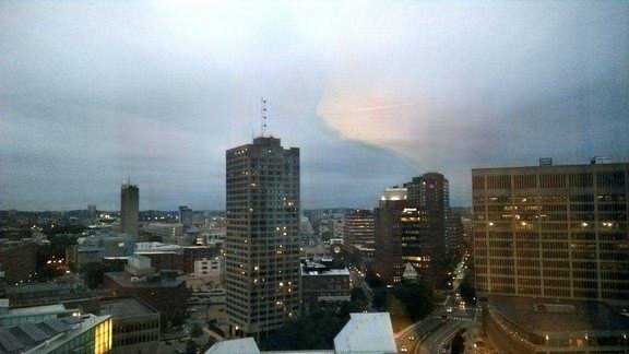
Our method has difficulty in handling complex scenes with multiple layers and highly dynamic objects. Fig. 18 shows that our method does not separate the reflection layer well. This example is particularly challenging as there are two layers of reflections: the top part contains the wooden beams, and the bottom part comes from the street behind the camera. Fig. 20 shows an example of a sequence containing a highly dynamic object (e.g., cat). As flow estimation cannot compensate for the motion well, our method produces blurry background reconstruction. Severe occlusions could also cause problems. In Fig. 20, we show a scene with severe adherent raindrops, which cause all methods to fail to remove the raindrops. In the blue zoom-in regions, our method successfully removes the adherent raindrops and recovers scene content better than DeRaindrop [65]. However, in the orange zoom-in regions, all methods fail to remove the adherent raindrops due to severe occlusions.
 |
Background |  |
 |
Reflection |  |
| Representative input frame | Our results |
5 Conclusions
In this work, we propose a novel method for multi-frame reflections and obstructions removal. Our key insight is to leverage a CNN to reconstruct background and reflection layers from flow-warped images. Integrating optical flow estimation and coarse-to-fine refinement enable our model to robustly recover the underlying clean images from challenging real-world sequences. Our method can be applied to different tasks such as fence or adherent raindrop removal with minimum changes in our design. We also show that online optimization on testing sequences leads to improved visual quality. Extensive visual comparisons and quantitative evaluation demonstrate that our approach performs well on a wide variety of scenes.
References
- [1] N. Arvanitopoulos, R. Achanta, and S. Susstrunk, “Single image reflection suppression,” in CVPR, 2017.
- [2] Q. Fan, J. Yang, G. Hua, B. Chen, and D. Wipf, “A generic deep architecture for single image reflection removal and image smoothing,” in ICCV, 2017.
- [3] M. Jin, S. Süsstrunk, and P. Favaro, “Learning to see through reflections,” in ICCP, 2018.
- [4] S. Jonna, K. K. Nakka, and R. R. Sahay, “Deep learning based fence segmentation and removal from an image using a video sequence,” in ECCV, 2016.
- [5] M. Park, K. Brocklehurst, R. T. Collins, and Y. Liu, “Image de-fencing revisited,” in ACCV, 2010.
- [6] K. Wei, J. Yang, Y. Fu, D. Wipf, and H. Huang, “Single image reflection removal exploiting misaligned training data and network enhancements,” in CVPR, 2019.
- [7] J. Yang, D. Gong, L. Liu, and Q. Shi, “Seeing deeply and bidirectionally: A deep learning approach for single image reflection removal,” in ECCV, 2018.
- [8] X. Zhang, R. Ng, and Q. Chen, “Single image reflection separation with perceptual losses,” in CVPR, 2018.
- [9] Y. Shih, D. Krishnan, F. Durand, and W. T. Freeman, “Reflection removal using ghosting cues,” in CVPR, 2015.
- [10] R. Szeliski, S. Avidan, and P. Anandan, “Layer extraction from multiple images containing reflections and transparency,” in CVPR, 2000.
- [11] E. Be’Ery and A. Yeredor, “Blind separation of superimposed shifted images using parameterized joint diagonalization,” TIP, vol. 17, no. 3, pp. 340–353, 2008.
- [12] C. Liu, J. Yuen, A. Torralba, J. Sivic, and W. T. Freeman, “Sift flow: Dense correspondence across different scenes,” in ECCV, 2008.
- [13] K. Gai, Z. Shi, and C. Zhang, “Blind separation of superimposed images with unknown motions,” in CVPR, 2009.
- [14] Y. Li and M. S. Brown, “Exploiting reflection change for automatic reflection removal,” in ICCV, 2013.
- [15] X. Guo, X. Cao, and Y. Ma, “Robust separation of reflection from multiple images,” in CVPR, 2014.
- [16] S. N. Sinha, J. Kopf, M. Goesele, D. Scharstein, and R. Szeliski, “Image-based rendering for scenes with reflections.” ACM TOG, vol. 31, no. 4, pp. 100–1, 2012.
- [17] A. Nandoriya, M. Elgharib, C. Kim, M. Hefeeda, and W. Matusik, “Video reflection removal through spatio-temporal optimization,” in ICCV, 2017.
- [18] C. Du, B. Kang, Z. Xu, J. Dai, and T. Nguyen, “Accurate and efficient video de-fencing using convolutional neural networks and temporal information,” in ICME, 2018.
- [19] J.-B. Alayrac, J. Carreira, and A. Zisserman, “The visual centrifuge: Model-free layered video representations,” in CVPR, 2019.
- [20] T. Xue, M. Rubinstein, C. Liu, and W. T. Freeman, “A computational approach for obstruction-free photography,” ACM TOG, vol. 34, no. 4, p. 79, 2015.
- [21] Y.-L. Liu, W.-S. Lai, M.-H. Yang, Y.-Y. Chuang, and J.-B. Huang, “Learning to see through obstructions,” in CVPR, 2020.
- [22] K. Gai, Z. Shi, and C. Zhang, “Blind separation of superimposed moving images using image statistics,” TPAMI, vol. 34, no. 1, pp. 19–32, 2011.
- [23] Y. Li and M. S. Brown, “Single image layer separation using relative smoothness,” in CVPR, 2014.
- [24] R. Wan, B. Shi, T. A. Hwee, and A. C. Kot, “Depth of field guided reflection removal,” in ICIP, 2016.
- [25] A. Punnappurath and M. S. Brown, “Reflection removal using a dual-pixel sensor,” in CVPR, 2019.
- [26] Y. Mu, W. Liu, and S. Yan, “Video de-fencing,” IEEE Transactions on Circuits and Systems for Video Technology, vol. 24, no. 7, pp. 1111–1121, 2013.
- [27] S. Jonna, S. Satapathy, and R. R. Sahay, “Stereo image de-fencing using smartphones,” in ICASSP, 2017.
- [28] R. Yi, J. Wang, and P. Tan, “Automatic fence segmentation in videos of dynamic scenes,” in CVPR, 2016.
- [29] S. Bell, K. Bala, and N. Snavely, “Intrinsic images in the wild,” ACM TOG, vol. 33, no. 4, p. 159, 2014.
- [30] T. Zhou, P. Krahenbuhl, and A. A. Efros, “Learning data-driven reflectance priors for intrinsic image decomposition,” in ICCV, 2015.
- [31] D. Eigen, C. Puhrsch, and R. Fergus, “Depth map prediction from a single image using a multi-scale deep network,” in NIPS, 2014.
- [32] J. Jeon, S. Cho, X. Tong, and S. Lee, “Intrinsic image decomposition using structure-texture separation and surface normals,” in ECCV, 2014.
- [33] E. Eisemann and F. Durand, “Flash photography enhancement via intrinsic relighting,” ACM TOG, vol. 23, no. 3, pp. 673–678, 2004.
- [34] T. Nestmeyer, J.-F. Lalonde, I. Matthews, and A. Lehrmann, “Learning physics-guided face relighting under directional light,” in CVPR, 2020.
- [35] Z. Li, M. Shafiei, R. Ramamoorthi, K. Sunkavalli, and M. Chandraker, “Inverse rendering for complex indoor scenes: Shape, spatially-varying lighting and svbrdf from a single image,” in CVPR, 2020.
- [36] S. Sengupta, J. Gu, K. Kim, G. Liu, D. W. Jacobs, and J. Kautz, “Neural inverse rendering of an indoor scene from a single image,” in ICCV, 2019.
- [37] S. Ilan and A. Shamir, “A survey on data-driven video completion,” Computer Graphics Forum, vol. 34, no. 6, pp. 60–85, 2015.
- [38] J.-B. Huang, S. B. Kang, N. Ahuja, and J. Kopf, “Temporally coherent completion of dynamic video,” ACM TOG, vol. 35, no. 6, p. 196, 2016.
- [39] R. Xu, X. Li, B. Zhou, and C. C. Loy, “Deep flow-guided video inpainting,” in CVPR, 2019.
- [40] C. Gao, A. Saraf, J.-B. Huang, and J. Kopf, “Deep flow-guided video inpainting,” in ECCV, 2020.
- [41] Y. Chen, C. Schmid, and C. Sminchisescu, “Self-supervised learning with geometric constraints in monocular video: Connecting flow, depth, and camera,” in ICCV, 2019.
- [42] X. Luo, J.-B. Huang, R. Szeliski, K. Matzen, and J. Kopf, “Consistent video depth estimation,” ACM TOG, vol. 39, no. 4, 2020.
- [43] Y. Sun, X. Wang, Z. Liu, J. Miller, A. A. Efros, and M. Hardt, “Test-time training for out-of-distribution generalization,” in ICML, 2020.
- [44] D. Ulyanov, A. Vedaldi, and V. Lempitsky, “Deep image prior,” in CVPR, 2018.
- [45] Y. Gandelsman, A. Shocher, and M. Irani, “Double-DIP: Unsupervised image decomposition via coupled deep-image-priors,” in CVPR, 2019.
- [46] Y.-C. Chen, C. Gao, E. Robb, and J.-B. Huang, “Nas-dip: Learning deep image prior with neural architecture search,” in ECCV, 2020.
- [47] Z. Kalal, K. Mikolajczyk, and J. Matas, “Tracking-learning-detection,” TPAMI, vol. 34, no. 7, pp. 1409–1422, 2011.
- [48] S. Hochreiter, A. S. Younger, and P. R. Conwell, “Learning to learn using gradient descent,” in International Conference on Artificial Neural Networks, 2001.
- [49] S. Ravi and H. Larochelle, “Optimization as a model for few-shot learning,” in ICLR, 2017.
- [50] O. Vinyals, C. Blundell, T. Lillicrap, D. Wierstra et al., “Matching networks for one shot learning,” in NIPS, 2016.
- [51] J. Snell, K. Swersky, and R. Zemel, “Prototypical networks for few-shot learning,” in NIPS, 2017.
- [52] V. Garcia and J. Bruna, “Few-shot learning with graph neural networks,” in ICLR, 2018.
- [53] H.-Y. Tseng, H.-Y. Lee, J.-B. Huang, and M.-H. Yang, “Cross-domain few-shot classification via learned feature-wise transformation,” in ICLR, 2020.
- [54] C. Finn, P. Abbeel, and S. Levine, “Model-agnostic meta-learning for fast adaptation of deep networks,” arXiv preprint arXiv:1703.03400, 2017.
- [55] A. Nichol and J. Schulman, “Reptile: a scalable metalearning algorithm,” arXiv preprint arXiv:1803.02999, vol. 2, no. 3, p. 4, 2018.
- [56] L. Zintgraf, K. Shiarli, V. Kurin, K. Hofmann, and S. Whiteson, “Fast context adaptation via meta-learning,” in ICML, 2019.
- [57] D. Sun, X. Yang, M.-Y. Liu, and J. Kautz, “Pwc-net: Cnns for optical flow using pyramid, warping, and cost volume,” in CVPR, 2018.
- [58] D. P. Kingma and J. Ba, “Adam: A method for stochastic optimization,” in ICLR, 2015.
- [59] A. Nichol, J. Achiam, and J. Schulman, “On first-order meta-learning algorithms,” arXiv preprint arXiv:1803.02999, 2018.
- [60] N. Xu, B. Price, S. Cohen, and T. Huang, “Deep image matting,” in CVPR, 2017.
- [61] T. Xue, B. Chen, J. Wu, D. Wei, and W. T. Freeman, “Video enhancement with task-oriented flow,” IJCV, vol. 127, no. 8, pp. 1106–1125, 2019.
- [62] R. Wan, B. Shi, L.-Y. Duan, A.-H. Tan, and A. C. Kot, “Benchmarking single-image reflection removal algorithms,” in ICCV, 2017.
- [63] R. Grosse, M. K. Johnson, E. H. Adelson, and W. T. Freeman, “Ground truth dataset and baseline evaluations for intrinsic image algorithms,” in ICCV, 2009.
- [64] Z. Wang, A. C. Bovik, H. R. Sheikh, E. P. Simoncelli et al., “Image quality assessment: from error visibility to structural similarity,” TIP, vol. 13, no. 4, pp. 600–612, 2004.
- [65] R. Qian, R. T. Tan, W. Yang, J. Su, and J. Liu, “Attentive generative adversarial network for raindrop removal from a single image,” in CVPR, 2018.
- [66] J. Yang, H. Li, Y. Dai, and R. T. Tan, “Robust optical flow estimation of double-layer images under transparency or reflection,” in CVPR, 2016.
![[Uncaptioned image]](/html/2008.04902/assets/author/yulunliu.jpg) |
Yu-Lun Liu is a Ph.D. candidate of Computer Science and Information Engineering at National Taiwan University, Taipei, Taiwan. He received the B.S. and M.S. degree in Electronics Engineering from National Chiao-Tung University, Hsinchu, Taiwan, in 2012 and 2014, respectively. His research interests include computer vision, machine learning, and multimedia. |
![[Uncaptioned image]](/html/2008.04902/assets/author/wslai.jpg) |
Wei-Sheng Lai is a software engineer at Google, working on mobile computational photography. He received the B.S. and M.S. degrees from the EE department at National Taiwan University in 2012 and 2014, respectively, and his Ph.D. degree from the EECS department at University of California, Merced in 2019. |
![[Uncaptioned image]](/html/2008.04902/assets/author/mhyang.jpg) |
Ming-Hsuan Yang is a Professor in Electrical Engineering and Computer Science at University of California, Merced. He served as an associate editor of the IEEE Transactions on Pattern Analysis and Machine Intelligence from 2007 to 2011, and is an associate editor of the International Journal of Computer Vision, Image and Vision Computing and Journal of Artificial Intelligence Research. Yang received the NSF CAREER award in 2012 and the Google Faculty Award in 2009. He is a Fellow of the IEEE. |
![[Uncaptioned image]](/html/2008.04902/assets/author/cyy.jpg) |
Yung-Yu Chuang received his B.S. and M.S. from National Taiwan University in 1993 and 1995 respectively, and the Ph.D. from the University of Washington at Seattle in 2004, all in Computer Science. He is currently a professor with the Department of Computer Science and Information Engineering, National Taiwan University. His research interests include computational photography, computer vision and rendering. |
![[Uncaptioned image]](/html/2008.04902/assets/author/jbhuang.jpg) |
Jia-Bin Huang is an assistant professor in the Bradley Department of Electrical and Computer Engineering at Virginia Tech. He received the B.S. degree in Electronics Engineering from National Chiao-Tung University, Hsinchu, Taiwan and his Ph.D. degree in the Department of Electrical and Computer Engineering at University of Illinois, Urbana-Champaign in 2016. |
