Extension of Full and Reduced Order Observers for Image-based Depth Estimation using Concurrent Learning

Abstract

In this paper concurrent learning (CL)-based full and reduced order observers for a perspective dynamical system (PDS) are developed. The PDS is a widely used model for estimating the depth of a feature point from a sequence of camera images. Building on the current progress of CL for parameter estimation in adaptive control, a state observer is developed for the PDS model where the inverse depth appears as a time-varying parameter in the dynamics. The data recorded over a sliding time window in the near past is used in the CL term to design the full and the reduced order state observers. A Lyapunov-based stability analysis is carried out to prove the uniformly ultimately bounded (UUB) stability of the developed observers. Simulation results are presented to validate the accuracy and convergence of the developed observers in terms of convergence time, root mean square error (RMSE) and mean absolute percentage error (MAPE) metrics. Real world depth estimation experiments are performed to demonstrate the performance of the observers using aforementioned metrics on a 7-DoF manipulator with an eye-in-hand configuration.

I Introduction

Estimating the 3D coordinates of feature points using observations from a sequence of camera images is referred to as the Structure from Motion (SfM) problem in computer vision literature. The 3D coordinates of feature points can be estimated by estimating the depth of the features. The estimated 3D coordinates of feature points or structure information can be used in a variety of automatic control, autonomy, and intelligent control applications. Existing solutions to this problem include offline [1] and online [2, 3, 4, 5, 6, 7, 8, 9, 10, 11, 12, 13, 14, 15, 16] methods. The focus of this paper is on online methods where the problem is formulated as a state estimation problem of a perspective dynamical system (PDS). The PDS is a class of nonlinear system that uses inverse depth parameterization, which is widely used in observer-based methods, and simultaneous localization and mapping (SLAM) [17].

Online methods often rely on the use of an Extended Kalman Filter (EKF) [5, 6]. In comparison to EKF-based approaches, nonlinear observers are developed for SfM with analytical proofs of stability. Under the assumption that the camera motion is known, continuous and discontinuous observers are developed to estimate the depth which can then be used to estimate the range to the object. A high-gain observer called the identifier-based observer is presented for range estimation in [7]. A semi-globally asymptotically stable reduced-order observer is presented in [8] to estimate the range based on immersion and invariance (I&I) methodology, which is extended to the range and orientation identification observer design in [18]. A continuous observer, which guarantees asymptotic range estimation, is presented in [9] under the assumption that camera motion is known. In [10], an asymptotically converging nonlinear observer is developed based on Lyapunov’s indirect method. In [11], a discontinuous sliding-mode observer is developed which guarantees exponential convergence of the estimation error. In [12], a nonlinear observer is developed that achieves local exponential convergence of estimation error. A range observer design based on nonlinear contraction and synchronization theory is presented in [19]. In [4], a globally exponentially stable observer is designed for the PDS. Extensions of these observers for PDS with moving objects are presented in [20, 21]. All these observers require persistence of excitation (PE) condition to be satisfied by the camera motion to achieve the convergence of the estimation error.

Drawing parallels to the adaptive control/observer design, in the PDS the inverse depth appears as a parameter in the dynamics of image-plane coordinates where the parameter is time-varying with known dynamics associated with it. Concurrent Learning (CL) is used in adaptive control for parameter estimation, where the knowledge of past trajectory data is leveraged to estimate the constant parameter and achieve state tracking [22, 23]. CL has also been used for target tracking applications in [24] and for target size estimation in [25]. The use of CL relaxes the PE condition to a finite excitation condition, which depends upon the rank of the regressor matrix [22].

Inspired by the recent advances in CL in adaptive control, full and reduced-order depth observers are proposed in the paper that builds on the work in [4]. The observer design guarantees the boundedness of the depth estimation error even when the PE condition is not satisfied by the camera motion in a time window given that finite excitation is present. The observer can be used to estimate the feature point depth to a desired accuracy. Two cases are analyzed for the convergence and stability of the observer design. The fist case is when the camera motions satisfy the PE condition and the second case is when the camera motions do not satisfy the PE condition. A Lyapunov stability analysis is carried out for the switched observer error system (i.e., when PE is satisfied and when it is not) using multiple Lyapunov functions [26]. Although compared to the existing depth/range observers in literature, the observers in this paper cannot achieve asymptotic or exponential depth estimation convergence, the observer can achieve finite estimation errors in practical scenarios when the existing observers may not yield finite estimation error. Practical examples include the motion of the camera along the projected ray while grasping an object or when an aerial robot is moving in the $Z$ direction during landing and takeoff or robots moving in the direction of view while docking. For these cases the camera motion will not satisfy the PE condition for certain time window. Compared to the recent work in [27, 28], a rigorous stability analysis and detailed simulation and experimental evaluations are presented in this paper. A history stack update procedure based on the Lyapunov analysis, which stores the camera motion and feature point data, is presented. The results of a performance evaluation of the CL-based full order and reduced order observers with a benchmark observer is presented using real world experiments conducted on camera mounted in the hand of 7 DoF Baxter robot.

II Perspective Camera Motion Model

The movement of a perspective camera capturing a scene results in the change of image plane coordinates of a feature point belonging to a static object. Let $\bar{m}(t)=\left[X(t)\>Y(t)\>Z(t)\right]^{T}\in\mathbb{R}^{3}$ and $m_{n}(t)=\left[\frac{X(t)}{Z(t)}\>\frac{Y(t)}{Z(t)}\>1\right]\in\mathbb{R}^{3}$ be the Euclidean and normalized Euclidean coordinates of a feature point belonging to a static object captured by a moving camera in the camera reference frame $\mathcal{F}_{C}$ with known camera velocities. To estimate the depth, define an auxiliary vector $\left[x(t)\>y(t)\>\chi(t)\right]^{T}\in\mathcal{Y}$ such that $\mathcal{Y}\subset\mathbb{R}^{3}$ is a closed and bounded set where $x(t)=\frac{X(t)}{Z(t)},y(t)=\frac{Y(t)}{Z(t)},\chi(t)=\frac{1}{Z(t)}$. Let $s(t)=\left[x\left(t\right)\>y\left(t\right)\right]^{T}$ be the state associated with an image plane feature point with two components and $\chi(t)$ be the inverse depth of the feature point.

Remark 1.

The state variables $x$ and $y$ are image plane coordinates of a feature point whose pixel coordinates are bounded by the resolution of the camera. As a result, the state variables $x(t)$ and $y(t)$ are bounded by known constants $\underline{x}\leq x(t)\leq\overline{x}$ and $\underline{y}\leq y(t)\leq\overline{y}$. The Euclidean distance $Z$(t) between the camera and the feature point can be lower bounded by the focal length of the camera $\lambda$ measured in meters and is not assumed to be upper bounded. Therefore, the inverse depth $\chi(t)$ can be upper and lower bounded as in [4, 12] using the constants $0<\underline{y_{3}}<\chi\leq\frac{1}{\lambda}$.

Assumption 1: The depth of the feature point $Z(t)$ is invertible in the compact set $\mathcal{Y}$.
The feature point dynamics can be written as a function of the linear and angular velocities as

$$\dot{s} =f_{m}(s,\omega)+\Omega^{T}(s,v)\chi$$ (1)

$$\dot{\chi} =f_{u}\left(s,\chi,u\right)$$ (2)

where $v\left(t\right)=\left[v_{X}(t)\>v_{Y}(t)\>v_{Z}(t)\right]^{T}\in\mathcal{V}$ , $\omega\left(t\right)=\left[\omega_{X}(t)\>\omega_{Y}(t)\>\omega_{Z}(t)\right]^{T}\in\mathcal{W}$ are the linear velocities in $\frac{\mathrm{m}}{\mathrm{s}}$ and angular velocities in $\frac{\mathrm{rad}}{\mathrm{s}}$ of the camera in the body frame and $u\left(t\right)=\left[v^{T}(t)\>\omega{}^{T}(t)\right]^{T}$. The sets $\mathcal{V}$ and $\mathcal{W}$ are bounded such that $\mathcal{V\subset\mathbb{R}}^{3}$ and $\mathcal{W\subset\mathbb{R}}^{3}$. In (1), $f_{m}(s,\omega)\in\mathbb{R}^{2}$ and $\Omega(s,v)\in\mathbb{R}^{1\times 2}$ are functions of measurable quantities or known quantities. The state derivative $\dot{s}\in\mathbb{R}^{2}$ is not measurable in this case and can only be estimated. Individually, $f_{m}(s,\omega)$, $\Omega(s,v)$, and $f_{u}(s,\chi,u)$ are defined as

$$f_{m}(s,\omega)=\left[\begin{array}[]{c}\begin{array}[]{ccc}xy&-\left(1+x^{2}\right)&y\\ 1+y^{2}&-xy&-x\end{array}\end{array}\right]\omega$$ (6)

$$\Omega(s,v)=\left[\begin{array}[]{c}\begin{array}[]{cc}xv_{Z}-v_{x}&yv_{Z}-v_{Y}\end{array}\end{array}\right]$$ (9)

$$f_{u}(s,\chi,u)=v_{Z}\chi^{2}+\left(y\omega_{X}-x\omega_{Y}\right)\chi$$ (10)

Problem Definition: Given the measurements of feature points in the image plane $s\left(t\right)$, the linear and angular velocity of the camera $u\left(t\right)$ and the linear acceleration of the camera $\dot{v}\left(t\right)$ in the camera reference frame, it is desired to estimate the inverse depth of the feature point $\chi\left(t\right)$ using the dynamics in (1)-(2). To this end, full order and reduced order depth observers are designed in Section III and Section V using CL.

Assumption 2: The camera velocities are bounded and the linear velocities are $\mathcal{C}^{1}$ with respect to time.

III CL-based Full Order Observer

The depth estimation schemes in the existing literature require a strong observability condition called Persistence of Excitation (PE). For such observers, the estimation error converges to zero only if the PE condition is satisfied. The PE condition is satisfied if there exist constants $T_{0},\rho\in\mathbb{R}^{+}$ such that

$$\int_{t}^{t+T_{0}}\Omega(s(\tau),v(\tau))\Omega^{T}(s(\tau),v(\tau))d\tau \geq\rho>0,\forall t>t_{0}.$$ (11)

CL based parameter estimation techniques use a history stack of recorded data generated by the dynamical system to make updates to the parameter estimation scheme. CL is based on the premise that even if the PE condition can not be guaranteed, input can be exciting over a finite interval of time. For the full order CL observer, the history stack is a tuple $\mathcal{H=}\left\{\left(\dot{\bar{s}}_{j},s_{j},u_{j}\right)\right\}_{j=1}^{M}$ containing the past data points up to the index $M-1$ chosen by the algorithm proposed in Section VII where $M$ is the index of the data point at the current time instant. Let $\left\{t_{j}\right\}_{j=1}^{M-1}$ denote the corresponding time instances at which the $j^{\mathrm{th}}$ entry in the history stack is recorded. Then by the definition of the history stack $\dot{\bar{s}}_{j}\coloneqq\dot{\bar{s}}\left(t_{j}\right),s_{j}\coloneqq s\left(t_{j}\right),u_{j}\coloneqq u\left(t_{j}\right)\>\forall j=1,\cdots,M-1$.

Assumption 3: The term $\dot{\bar{s}}_{j}$ is the approximation of $\dot{s}_{j}$ using computed numerically such that $\|\dot{\bar{s}}-\dot{s}\|<\bar{d}$ and $\bar{d}\in[0,\infty)$ is an unknown constant.

The estimates of $s,\chi$ are denoted by $\hat{s},\hat{\chi}$ respectively and the state and depth estimation errors as $z=\chi-\hat{\chi},$ and $\xi=s-\hat{s}$. Using the dynamics in (1) and (2), the observer for estimating the state and the depth is designed as follows.

$$\dot{\hat{s}}= f_{m}(s,\omega)+\Omega^{T}(s,v)\hat{\chi}+H\xi$$ (12)

$$\dot{\hat{\chi}}= f_{u}(s,\hat{\chi},u)+\Gamma\Omega(s,v)\xi+K_{CL}\Gamma\sum_{j=1}^{M}\Omega(s_{j},v_{j})(\dot{\bar{s}}_{j}$$

$$-f_{m}(s_{j},\omega_{j})-\Omega^{T}(s_{j},v_{j})\hat{\chi})$$ (13)

where $H\in\mathbb{R}^{2\times 2}$ is positive definite diagonal gain matrix, $\Gamma\in\mathbb{R}^{+}$ and $K_{CL}\in\mathbb{R^{+}}$ are suitable observer gains. Since $d_{j}=\dot{\bar{s}}_{j}-\dot{s}_{j}$, the approximated state derivative term $\dot{\bar{s}}_{j}$ is substituted as $\dot{\bar{s}}_{j}=f_{m}(s_{j},\omega_{j})+\Omega^{T}(s_{j},v_{j})\chi_{j}+d_{j}$ to compute the estimation error dynamics. Using the observer equations in (12)-(13), adding and subtracting $K_{CL}\Gamma\sum_{j=1}^{M}\Omega(s_{j},v_{j})\Omega^{T}(s_{j},v_{j})\chi$, grouping $\chi$ and $\hat{\chi}$, the estimation error dynamics can be written as

$$\dot{\xi}= -H\xi+\Omega^{T}(s,v)z$$

$$\dot{z}= -\Gamma\Omega(s,v)\xi+g(s,z,u)-K_{CL}\Gamma\big{(}\sum_{j=1}^{M}\Omega(s_{j},v_{j})d_{j}$$

$$+\sum_{j=1}^{M}\Omega(s_{j},v_{j})\Omega^{T}(s_{j},v_{j})\left(z+\chi_{j}-\chi\right)\big{)}$$ (14)

where $g(s,z,u)=f_{u}(s,\chi,u)-f_{u}(s,\hat{\chi},u)$.

Assumption 4: The history stack contains recent information and the change in depth over a short period of time remains bounded i.e., $\exists\bar{\chi}\geq 0$ such that $\sup_{t\geq 0}\mathrm{max}_{j\in\left\{1,\cdots,M-1\right\}}\|\chi_{j}-\chi\|\leq\bar{\chi}$, where $\chi_{j}=\chi\left(t_{j}\right)$ and $\chi$ are the past and current true depth values at the time instants $t_{j}$ and $t$ such that $t>t_{j}\quad\forall j=1,\cdots,M-1$ for a suitably chosen value of $M$.

Remark 2.

The main implication of Assumption 4 is that the history stack should be frequently updated to contain information about the current true depth from the past feature point and camera motion data. Additionally, the upper bound $\bar{\chi}$ will be smaller if the object is not too close to the camera and the camera linear velocities are slow.

IV Stability Analysis for Full Order Observer

Since the history stack is initialized with zeros, the stability analysis is carried out in two phases, viz., the initial phase when the data is being collected in the history stack and the phase when the history stack is fully populated with informative points. In Theorem 1, leveraging our prior work in [4], it is shown that the estimation error dynamics in (14) are stable and yield a UUB error under a PE condition when the history stack is incomplete. In Theorem 2, it is shown that the estimation error dynamics in (14) yield UUB error when the PE condition is not satisfied and the history stack is complete. The advantage of adding the CL term is that the error is bounded even if the PE condition is not satisfied. To facilitate the analysis, let $\exists\bar{\sigma}>0$ such that $\sup_{t\geq 0}\max_{j\in\left\{1,\cdots,M\right\}}\|\Omega(s_{j},v_{j})\Omega^{T}(s_{j},v_{j})\|\leq\bar{\sigma}$ and $\text{$\sigma_{1}$}=\sum_{j=1}^{M-1}\Omega(s_{j},v_{j})\Omega^{T}(s_{j},v_{j})$ such that $\sigma_{1}\in\mathbb{R}_{\geq 0}$.

Definition 1.

The history stack is defined to be incomplete when the stack is not completely populated with informative points such that $\sigma_{1}\geq 0.$

Definition 2.

The history stack is defined to be complete when the history stack is completely populated with informative points such that $\sigma_{1}>0.$

Theorem 1.

When the history stack is incomplete, the error system in (14) is UUB if Assumption 4 and the PE condition in (11) are satisfied. Further, the ultimate bound on the estimation error is given by $\sqrt{\frac{c_{2}}{c_{1}}}\frac{\gamma_{1}K_{CL}\Gamma((M-1)\bar{\sigma}\bar{\chi}+M\bar{d}\sqrt{\bar{\sigma}})}{k_{2}}$, where $c_{1},c_{2},k_{2},\gamma_{1}$ are positive constants.

Proof:

Refer Appendix $A$. ∎

Theorem 2.

When the history stack is complete, the error system in (14) is UUB if Assumption 4 is satisfied, the PE condition in (11) is not satisfied, and the adjustable observer gain is selected according to the sufficient condition, $K_{CL}>\frac{L_{g}}{\sigma_{1}\Gamma}$. Further, the ultimate bound on the estimation error is given by $\sqrt{\frac{c_{4}}{c_{3}}}\frac{K_{CL}((M-1)\bar{\sigma}\bar{\chi}+M\bar{d}\sqrt{\bar{\sigma}})}{\sqrt{2k_{3}\alpha_{1}}}$, where $c_{3},c_{4},k_{3},\alpha_{1}$ are positive constants.

Proof:

Refer Appendix $B$. ∎

V CL-based Reduced Order Observer

For the reduced order CL observer, the history stack is a tuple $\mathcal{H=}\left\{\left(s_{j},u_{j},\dot{v}_{j}\right)\right\}_{j=1}^{M}$ containing the past data points up to the index $M-1$ chosen by the algorithm detailed in Section VII where $M$ is the index of the data point at the current time instant. The reduced order depth observer is defined as

$$\hat{\chi}\left(t\right)=\kappa\left(s,\hat{\chi},u,\dot{v}\right)+\gamma\left(s,v\right)$$ (15)

where

$$\dot{\kappa} =f_{u}(s,\hat{\chi},u)+\bar{K}\sum_{j=1}^{M}\biggl{(}\theta_{j}^{T}\dot{v}_{j}$$

$$\quad-\Omega(s_{j},v_{j})\left(f_{m}(s_{j},\omega_{j})+\Omega^{T}(s_{j},v_{j})\hat{\chi}\right)\biggr{)}$$

$$\gamma =-\bar{K}\sum_{j=1}^{M}\theta_{j}^{T}v_{j}$$ (16)

where $\theta_{j}=\left[x_{j}\;y_{j}\;\frac{-(x_{j}^{2}+y_{j}^{2})}{2}\right]^{T}$ for $j=1,\cdots,M$. The initial condition of the observer is selected as $\kappa(t_{0})=\kappa_{0}$ where $\kappa_{0}>0$ is a constant.

VI Stability Analysis for Reduced Order Observer

Differentiating (15) and using (16), to obtain the dynamics of $\hat{\chi}(t)$ as

$$\dot{\hat{\chi}}\negthickspace =\negthickspace f_{u}\left(s,\hat{\chi},u\right)\negthickspace+\negthickspace\bar{K}\negmedspace\sum_{j=1}^{M}\negthickspace\Omega\left(s_{j},v_{j}\right)\negthinspace\left(\negthinspace\dot{s}_{j}\negthickspace-\negthickspace f_{m}(s_{j},\omega_{j})\negthickspace-\negthickspace\Omega^{T}(s_{j},v_{j})\hat{\chi}\right).\negthickspace$$ (17)

The error dynamics for the reduced order observer can be derived by using (10), (17), substituting $\dot{s}_{j}$ from (1), adding and subtracting $\bar{K}\sum_{j=1}^{M}\Omega(s_{j},v_{j})\Omega^{T}(s_{j},v_{j})\chi$, and grouping $\chi$ and $\hat{\chi}$ as

$$\dot{z}\negthickspace =-\bar{K}\negthickspace\left(\sum_{j=1}^{M}\negthickspace\Omega(s_{j},v_{j})\Omega^{T}(s_{j},v_{j})\left(z\negthickspace+\negthickspace\chi_{j}\negthickspace-\negthickspace\chi\right)\negthickspace\right)\negthickspace+g(s,z,u),$$ (18)

where $g(s,z,u)=f_{u}(s,\chi,u)-f_{u}(s,\hat{\chi},u)$. Similar to the case of the full order CL-based observer, the stability analysis of the reduced order CL-based observer is carried out in two phases viz. the initial phase when the data is being collected in the history stack and the phase when the history stack is fully populated with informative points. In Theorem 3, it is shown that the estimation error dynamics in (18) are stable and yield a UUB error under a PE condition when the history stack is incomplete. In Theorem 4, it is shown that the estimation error dynamics in (18) yield UUB error when the PE condition is not satisfied and the history stack is complete.

Theorem 3.

When the history stack is incomplete, the error system in (18) is UUB if Assumption 4 and the PE condition in (11) are satisfied. Further, the ultimate bound on the estimation error is given by $\sqrt{\frac{c_{6}}{c_{5}}}\frac{\gamma_{2}\bar{K}\bar{\sigma}(M-1)\bar{\chi}}{k_{4}}$, where $c_{5},c_{6},k_{4},\gamma_{2}$ are positive constants.

Proof:

Refer Appendix $C$. ∎

Theorem 4.

When the history stack is complete, the error system in (18) is UUB if Assumption 4 is satisfied, the PE condition in (11) is not satisfied, and the adjustable observer gain is selected according to the sufficient condition, $\bar{K}>\frac{L_{g}}{\sigma_{1}}$. Further, the ultimate bound on the estimation error is given by $\frac{\bar{K}\bar{\sigma}(M-1)\bar{\chi}}{k_{5}}$, where $k_{5}$ is a positive constants.

Proof:

Refer Appendix $D$. ∎

Remark 3.

The gains $\bar{K}$ and $K_{CL}$ can be chosen to minimize the effect of $z^{T}g(s,z,u)$. For the full order and the reduced order observer, the estimation error decreases exponentially to an ultimate bound as $t\to\infty$. The ultimate bound on the estimation error can be made arbitrarily small by selecting appropriate gain values $H$, $\Gamma$, $K_{CL}$ for the full order observer, or $\bar{K}$ for the reduced order observer, and the size of the history stack $M$. The optimal observer gains may be efficiently computed by solving a Linear Matrix Inequality using incremental quadratic constraints as demonstrated in [29].

Remark 4.

Old data can be replaced with new data in the history stack even after the history stack is full as long as $\sigma_{1}$ is greater than zero. Using the procedure in Section VII, $\sigma_{1}$ always stays positive even after the old points are replaced from the full history stack. Hence, the upper bound on the derivative of the Lyapunov functions for the full and reduced order observers holds at any given time after the history stack is full. Thus, the ultimate bound on the switched systems can be derived from analysis of multiple Lyapunov functions as demonstrated in Thm 3.1 of [26].

Remark 5.

The ultimate bound on the estimation error $\iota_{b}$ increases linearly with $\bar{\chi}$, defined in Assumption 4. As a result, if the history stack contains old points with previous values, the ultimate bound on the estimation error will grow linearly with $\bar{\chi}$. Hence, it is essential for the history stack to be updated frequently to avoid the growth of the ultimate bound. Based on the presented analysis, Algorithm I is designed to frequently update the history stack and ensure that $\sigma_{1}$ stays greater than zero.

VII History Stack Update

From the analysis in Sections IV and VI, an algorithm is designed in this section to ensure the ultimate bound on the error is small and that $\sigma_{1}$ stays positive. Auxiliary stacks $\mathcal{G=}\{(\dot{\bar{s}}_{j,}s_{j},u_{j})\}_{j=1}^{N}$ for the full order observer and $\mathcal{G=}\{(s_{j},u_{j},\dot{v}_{j})\}_{j=1}^{N}$ for the reduced order observer, such that $N>M$, are used to select informative points. The auxiliary stack is a dynamic sliding window of the $N$ most recent points. In each iteration, $M-1$ most informative points are selected from the auxiliary stack to replace all the points in the history stack. The history stack and auxiliary stack are both initialized with zeros. At each time instance, the auxiliary stack is sorted in descending order based on the value of $\Omega(s_{j},v_{j})\Omega^{T}(s_{j},v_{j})\quad\forall j=1,\cdots,N$ to select the top $M-1$ points. The points in the history stack are replaced only if the chosen $M-1$ points from the auxiliary stack satisfy $\{\sum_{j=1}^{M-1}\Omega\Omega^{T}\}_{\mathcal{G}}\geq\epsilon$ for a suitably chosen constant $\epsilon>0$. This, ensures that the value of $\sigma_{1}$ does not drop below $\epsilon$ and the upper bound on the derivative of the Lyapunov functions in (23) and (29) holds at all times after the history stack is full. The choice of $\epsilon$ is critical as it maintains a balance between frequently updating the stack and ensuring that $\sigma_{1}$ remains greater than zero.

if data is available then

       if ${\mathcal{H}}$ is not full then

             Add data point to History Stack ${\mathcal{H}}$;

            

       end if

      Add data point to ${\mathcal{G}}$ in a cyclic way;

       if ${\mathcal{H}}$ is full then

             Search for ${M-1}$ data points with maximum ${\{\Omega\Omega^{T}\}}$ in the ${\mathcal{G}}$ stack;

             if ${\{\sum_{j=1}^{M-1}\Omega\Omega^{T}\}}_{\mathcal{G}}\geq\epsilon$ then

                   ${\mathcal{H}\leftarrow\mathcal{G}}$ for the selected ${M-1}$ points;

                  

             end if

            

       end if

      

end if

Algorithm 1 Algorithm to update History Stack

VIII Simulation Results

VIII-A Simulation 1

A simulation is performed using a simulated feature point to verify the performance of the CL full order observer designed in Section III. An initial point with Euclidean coordinates $\bar{m}(t_{0})=\left[2.5\>0.5\>3\right]{}^{T}$ is selected. A fourth order Runge-Kutta (R-K) ODE solver with a fixed time-step of $\frac{1}{30}\mathrm{s}$ ($30\mathrm{fps}$) is used to integrate the equations and generate trajectories for all values of $\bar{m}(t)$. In this simulation, the linear velocities are designed as $v=\left[0.3\>0.2\mathrm{cos}(\frac{\pi t}{4})\>-0.3\right]^{T}$and $\omega=\left[0\>-\frac{\pi}{30}\>0\right]^{T}$.

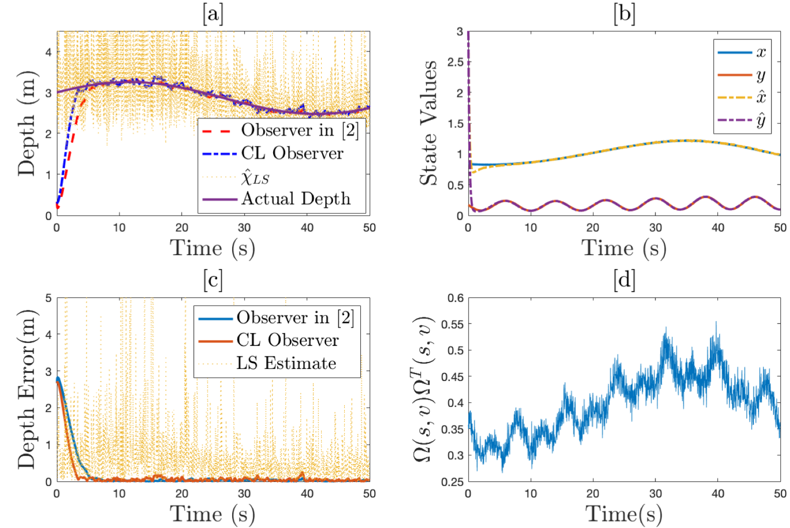
Figure 1: (a) Comparison between the actual depth and estimated depth over a period of 50 seconds. (b) Comparison between the actual and estimated state values. (c) Error between the true and the estimated depth. (d) Evolution of $\Omega(s,v)\Omega^{T}(s,v)$ for the simulated velocities and described initial conditions.

Additive white Gaussian noise with a signal to noise ratio (SNR) of 40 dB is added to the states and the velocity measurements are corrupted with a Gaussian distributed measurement noise with zero mean and variance of 0.01. The CL full order observer gain values used for the simulation are $K_{CL}=0.15$, $\Gamma=5,$ $H=\mathrm{diag\{10,10\}}$. The initial values for the state estimate and inverse depth estimate are selected as $\hat{s}(t_{0})=\left[10\>5\right]^{T}$ and $\hat{\chi}(t_{0})=3$ which corresponds to a depth of $0.33\mathrm{m}$. The history stack and the auxiliary stack are initialized with three points and five points respectively. The CL full order observer converges to the true depth in $4.7\>\mathrm{s}$ as shown in Figure 1(a). Figure 1(b) shows the actual state trajectories and the estimated state trajectories estimated by the CL full order observer. The yellow dashed lines in Figure 1(a) show the performance of the least squares (LS) depth estimation based on the formula $\hat{\chi}_{LS}=(\Omega^{T}(s,v))^{\dagger}(\dot{\bar{s}}-f_{m}(s,\omega))$. Figure 1(c) shows the corresponding error plots for the CL observer, the batch LS estimator and the observer in [2]. A simple least squares estimation is not a good solution to the depth estimation problem due to the measurement noise and the singular value of $\Omega$. The accuracy for the CL observer, batch LS estimator and the observer in [2] is reported for 500 Monte Carlo runs of a 50s simulation. Initial conditions are sampled from a normal distribution centered around $\hat{s}(t_{0})=[10,5]^{T}$ and $\hat{\chi}(t_{0})=3$. The CL full order observer achieves steady state root mean square error (RMSE) of $0.046\mathrm{m}$ and mean absolute percentage error (MAPE) of $1.83\%$. The LS estimation achieves RMSE of $1.05\mathrm{m}$ and MAPE of $23.18\%$. The observer in [2] converges in $6.46\>\mathrm{s}$ and achieves RMSE of $0.024\mathrm{m}$ and MAPE of $1.05\%$ when the gains are set to $\mathbf{\Lambda}=9,\boldsymbol{H}=\mathrm{diag\{10,10\}},\boldsymbol{Q}=\mathrm{diag}\left\{4,4\right\}$.

VIII-B Simulation 2

In this simulation the PE condition is violated between $31\mathrm{s}-\mathrm{38\mathrm{s}}$. An initial point with Euclidean coordinates $\bar{m}(t_{0})=\begin{array}[]{c}\left[1\>1\>1\right]^{T}\end{array}$ used to generate the trajectories using the velocities in simulation 1 from 0s to 31s. Since PE depends only on linear velocities, they are chosen such that $\Omega(s,v)\Omega^{T}(s,v)=0$ at each time instant during the period $31\mathrm{s}-38\mathrm{s}$. This implies that $v_{X}=xv_{Z}$ and $v_{Y}=yv_{Z}$ at each time instant. The linear velocity in the $Z$ direction is chosen to be $v_{Z}=0.1\mathrm{cos}(\frac{\pi t}{4})\mathrm{m/s}$ and the angular velocities are set to $0\>\mathrm{rad/s}$. As a result, the linear and angular velocities are $v=\begin{array}[]{c}\left[\frac{x(t)}{10}\mathrm{c}_{1},\;\frac{y(t)}{10}\mathrm{c}_{1},\;\frac{1}{10}\mathrm{c}_{1}\right]\end{array}^{T}$and $\omega=\left[0\>0\>0\right]^{T}$ where $\mathrm{c}_{1}=\mathrm{cos}(\frac{\pi t}{4})$. For PE violation, the initial condition is set to the state at $31\mathrm{s}$ i.e $\bar{m}(t_{31})$. Once the PE violation stops at $38\mathrm{s}$, the velocities in simulation 1 are used for simulating the trajectories up to $50\mathrm{s}$. Additive white Gaussian noise with SNR $20\mathrm{dB}$ is added to the pixel measurements and Gaussian distributed noise with zero mean and variance 0.01$\frac{\mathrm{m^{2}}}{\mathrm{s^{2}}}$ for the linear velocities and 0.01$\frac{\mathrm{rad}^{2}}{\mathrm{s^{2}}}$ for the angular velocities is added to the velocity measurements.

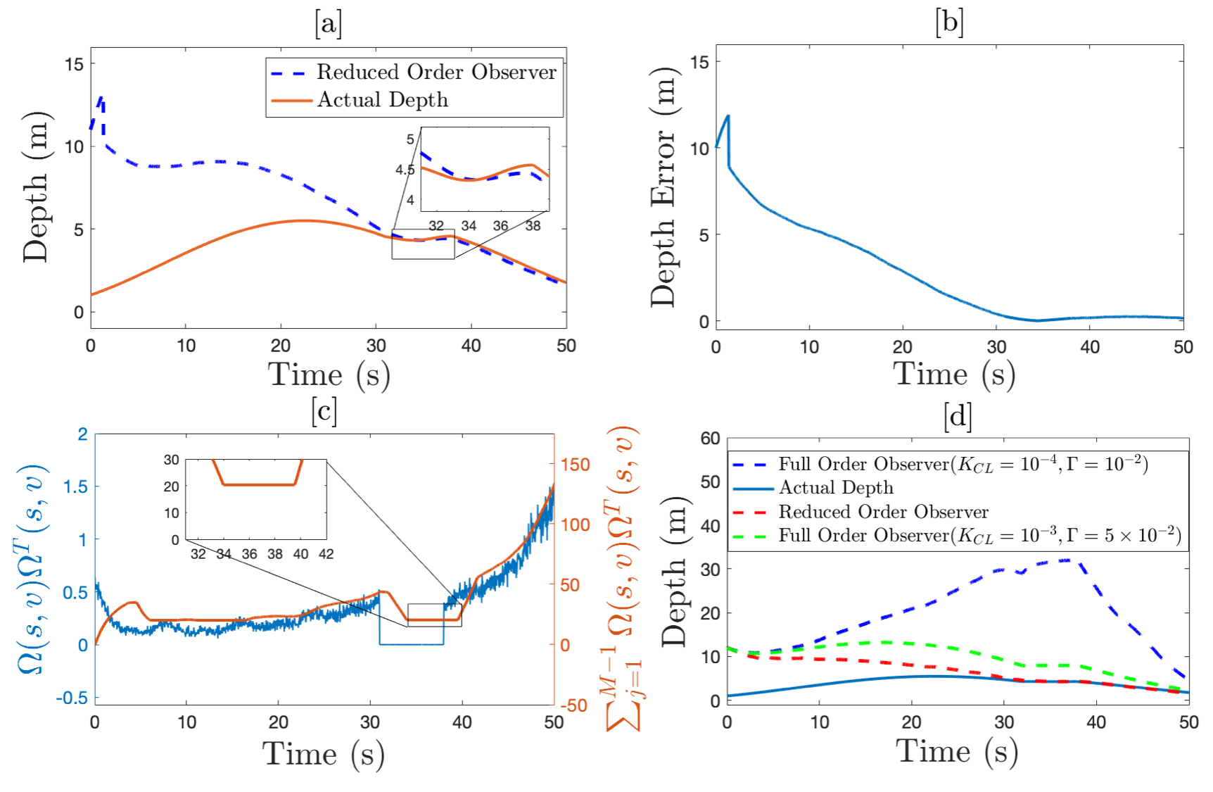
Figure 2: (a) Comparison of true vs estimated depth using reduced order observer. (b) Depth estimation error for reduced order observer. (c) Evolution of $\Omega(s,v)\Omega^{T}(s,v)$ with time showing the PE violation from $t=31\mathrm{s}$ to $38\mathrm{s}$. (d) Comparison between reduced order integrated observer and CL observer for different gain values in the presence of $20\mathrm{dB}$ noise.

The numerically approximated value of the PE between 31s to 38s is $\intop_{31}^{38}\Omega(s(\tau),v(\tau))\Omega^{T}(s(\tau),v(\tau))d\tau=7.83\times 10^{-4}$. Figure 2(a) shows the performance of the predicted depth by the CL reduced order observer. The history stack is chosen to hold $120$ points corresponding to $4\mathrm{s}$ of data and the auxiliary stack is chosen to hold $150$ points corresponding to a window of $5\mathrm{s}$. The observer is initialized at $\hat{s}(t_{0})=\left[1\;1\right]^{T}$ and $\hat{\chi}(t_{0})=0.08$ which corresponds to actual depth of $12\mathrm{m}$. The gain $\bar{K}$ for the reduced order observer is set to $2\times 10^{-3}$. From Figure 2(b) the CL reduced order observer error exponentially converges to an ultimate bound at $35.9\mathrm{s}$, during the period when the PE condition is violated. The value of $\sigma_{1}=\sum_{j=1}^{M-1}\Omega(s_{j},v_{j})\Omega^{T}(s_{j},v_{j})$ always remains greater than zero once the history stack is full. The value of $\sigma_{1}$ does not drop below $\epsilon$ defined in Algorithm 1. The value of $\epsilon$ is chosen to be $20\mathrm{}$ and to maintain this value the history stack is not updated between 34s to 40s as shown in Figure 2(c). The steady state RMSE achieved is $0.129\mathrm{m}$ and steady state MAPE achieved is $3.61\%$. Figure 2(d) shows the comparison of the CL full order observer presented in Section III with the CL reduced order observer when the state measurements are noisy.

IX Experiments

IX-A Experimental Platform

The camera in the wrist of the right arm of a Baxter research robot is used to capture images containing the feature point at a rate of 30 fps with resolution 640x400. The centroid of white circle is used against a black background for easy thresholding based image segmentation. The processing of the images and depth estimation is done in MATLAB 2019a at $30\>\mathrm{fps}$ using a desktop with Intel Core2Duo CPU with clock-speed of 2.26 GHz and 4 GB RAM running Ubuntu 14.04. The camera intrinsics for Baxter’s right hand camera obtained through the Baxter API and Robot Operating System (ROS) are given by $f_{x}=f_{y}=407.1$, $c_{x}=323.4$ and $c_{y}=205.6$ where $\left(c_{x},c_{y}\right)$ represents the camera center pixel. The ground truth depth for comparing the results is obtained using simple pose transformations as the pose of the coordinate frame attached to camera and the feature point is known in the coordinate frame attached to the base of the robot.

IX-B Results

The experiment is done for 16 seconds wherein the camera is stationary for the first $1.5\mathrm{s}$. After $1.5\mathrm{s}$ the camera starts moving in a circular motion in the $XY$ plane up to $5.5\mathrm{s}.$ After $5.5\mathrm{s}$ the camera moves downward along the $Z$ direction and back for time up to $10\mathrm{s}.$ The motion from $10\mathrm{s}-15\mathrm{s}$ is circular in the $XY$ plane followed by a downward motion along the $Z$ direction. The estimated depth by full and reduced order observers, and the observer in [2] is shown in Figure 3(a). The observers are initialized with initial conditions $\hat{s}(t_{0})=\left[1\;1\right]^{T}$ and $\hat{\chi}(t_{0})=2.5$ which corresponds to a depth of $0.4\mathrm{m}$.

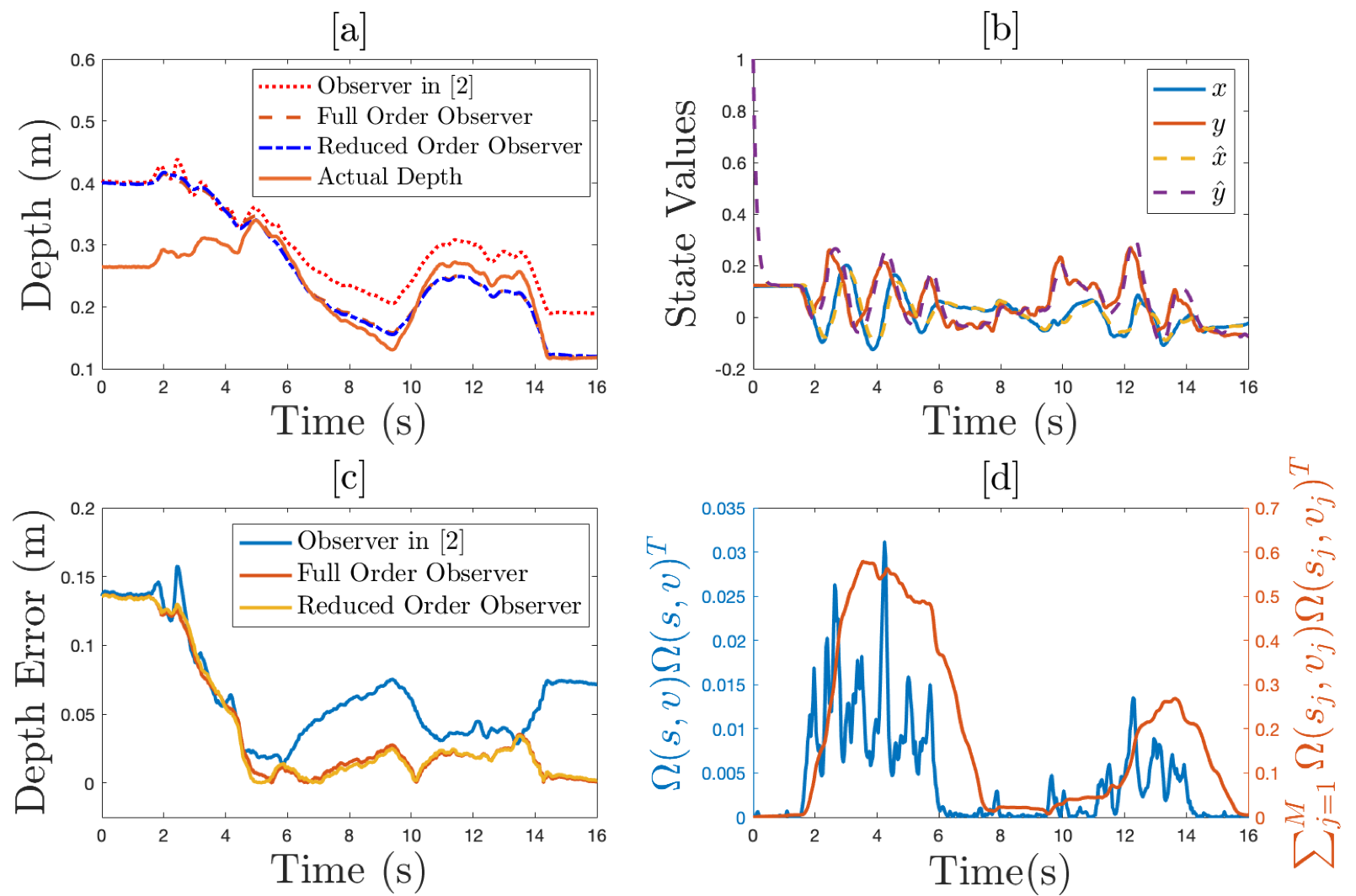
Figure 3: (a) Comparison of true depth vs estimated depth using full order and reduced order observer. (b) Comparison between the actual and estimated state values using full order observer. (c) Depth estimation error for full and reduced order observer. (d) Evolution of $\Omega(s,v)\Omega^{T}(s,v)$ and $\sum_{j=1}^{M}\Omega(s_{j},v_{j})\Omega^{T}(s_{j},v_{j})$ with time.

The depth estimation error exponentially converges to an ultimate bound as shown in Figure 3(c). The camera moves in the $XY$ plane from $1.5\mathrm{s}-5.5\mathrm{s}$ and the value of $\intop_{1.5}^{5.5}\Omega(s(\tau),v(\tau))\Omega^{T}(s(\tau),v(\tau))d\tau=4.12\times 10^{-2}$ is approximated numerically using trapezoidal rule of integration. When PE is violated $\intop_{6}^{10}\Omega(s(\tau),v(\tau))\Omega^{T}(s(\tau),v(\tau))d\tau=2.15\times 10^{-3}\mathrm{}$, also the maximum value of $\Omega(s,v)\Omega^{T}(s,v)$ is $0.035$ at $4.03\mathrm{s}$. The violation of the PE condition is achieved by moving the camera along $Z$ direction when the feature point is exactly at the centre of the image implying that $s\thickapprox 0$. The value of the estimated image plane feature point coordinates by the observer in (12) compared to the true values are shown in Figure 3(b). The value of the constant is chosen as $\epsilon=0.03$ and $\sigma_{1}\geq\epsilon$ as shown in Figure 3(c) even when PE is not satisfied. The full order observer converges in $4.7\mathrm{s}$ and achieves RMSE of $0.016\mathrm{m}$ and MAPE of $6.55\%$. The reduced order observer converges in $4.7\mathrm{s}$ and achieves RMSE of $0.015\mathrm{m}$ and MAPE of $6.28\%$. The estimation error keeps decreasing in the first $6\mathrm{s}$ for the observer in [2] when the camera motion is informative. However, the observer does not converge after $6\mathrm{s}$ when the motion is not informative. The observer in [2] achieves RMSE of $0.046\mathrm{m}$ and MAPE of $26.11\%$ when the gains are set to $\mathbf{\Lambda}=60,\boldsymbol{H}=\mathrm{diag\{30,30\}},\boldsymbol{Q}=\mathrm{diag}\left\{6,6\right\}$.

X Conclusion

CL based full order and reduced order nonlinear observers are presented in Section III and Section V for estimating the depth of a stationary feature point in an image using a moving camera. The estimation errors for the full order observer and reduced order observer are shown to be UUB. An analytical expression is derived for the ultimate bound on the error for the presented observers. Based on the stability analyses, an algorithm to update the history stack is designed in Section VII. The algorithm ensures convergence of the error states and frequent update of the history stack used for CL. The developed observers and algorithm are verified through numerical simulations in Section VIII-A and Section VIII-B. The observers are successfully tested in real world experiments on a Baxter research robot when PE is violated and the camera motions are not informative. Despite the promising results, the choice of the sizes of the history and auxiliary stacks, the observer gains, and $\epsilon$ are purely empirical. The optimal choice of these parameters is a topic for the future. The depth observer design for discrete time systems will also be explored as a part of the future work.

Lemma 1.

The function $g(s,z,u)$ is Lipschitz continuous with respect to the variable $z$ with a Lipschitz constant $L_{g}$.

Proof:

For a single feature point , $g(s,z,u)=f_{u}(s,\chi,u)-f_{u}(s,\hat{\chi},u)$. Using the definition of $f_{u}(s,\chi,u)$ in (10)

$$\|g(s,z,u)\| =\|f_{u}(s,\chi,u)-f_{u}(s,\hat{\chi},u)\|$$

$$=\|\chi^{2}v_{Z}+(y\omega_{X}-x\omega_{Y})\chi$$

$$\quad-(\hat{\chi}^{2}v_{Z}+(y\omega_{X}-x\omega_{Y})\hat{\chi})\|$$

$$=\|(\chi^{2}-\hat{\chi}^{2})v_{Z}+(y\omega_{X}-x\omega_{Y})(\chi-\hat{\chi})\|$$

$$=\|(\chi+\hat{\chi})v_{Z}z+(y\omega_{X}-x\omega_{Y})z\|$$

$$=\|\left((\chi+\hat{\chi})v_{Z}+(y\omega_{X}-x\omega_{Y})\right)z\|$$

Using Assumption 2 and Remark 1, $g(\cdot)$ can be upper bounded as

$$\|g(s,z,u)\| \leq\|(\chi+\hat{\chi})v_{Z}+(y\omega_{X}-x\omega_{Y})\|\|z\|$$

$$\leq L_{g}\|z\|$$

The boundedness of $\hat{\chi}$ is ensured through the locally Lipschitz projection law described in [4]. ∎

A. Proof of Theorem 1
Consider a domain $\mathcal{D}\subset\mathbb{R}^{3}$ containing $e(0)=[\xi(0),z(0)]^{T}$. In the subsequent development, the result of Proposition 1 in [12] is used which proves the existence of a candidate Lyapunov function $V(t,e):\mathcal{D}\rightarrow\mathbb{R}^{+}$ which can be upper and lower bounded by $c_{1}\|e\|^{2}\leq V(t,e)\leq c_{2}\|e\|^{2}$ such that $c_{1},c_{2}>0$ and satisfies $\|\frac{\partial V}{\partial e}\|\leq\gamma_{1}\|e\|$. The derivative of the Lyapunov function guarantees the exponential stability of the estimation error dynamics without the CL terms when the PE condition in (11) is satisfied. Using the triangle inequality and Cauchy-Schwartz inequality an upper bound is derived as $\sum_{j=1}^{M-1}\Omega(s_{j},v_{j})\Omega^{T}(s_{j},v_{j})(\chi_{j}-\chi)\leq\bar{\sigma}\sum_{j=1}^{M-1}\|\chi_{j}-\chi\|$. Using the Lipschitz continuity property (refer Lemma 1), the term $g(s,z,u)$ can be upper bounded by $\|g(s,z,u)\|\leq L_{g}\|z\|$, where $L_{g}$ is the Lipschitz constant. Using the Cauchy-Schwartz inequality and Lipschitz continuity of $g(s,z,u)$, the upper bounds on the term $z^{T}g(s,z,u)$ can be derived as follows.

$$\|z^{T}g(s,z,u)\|\leq L_{g}\|z\|{}^{2}$$ (19)

When the history stack is incomplete, $\sigma_{1}\geq 0$. Using Assumption 3-4, result of Proposition 1 of [12], completing the squares, the derivative of the Lyapunov function can be upper bounded as

$$\dot{V} \leq-\frac{k_{2}}{2c_{2}}V+\frac{\gamma_{1}^{2}K_{CL}^{2}\Gamma^{2}((M-1)\bar{\sigma}\bar{\chi}+M\bar{d}\sqrt{\bar{\sigma}})^{2}}{2k_{2}}$$ (20)

for $k_{2}>0$. Using the comparison lemma 3.4 from [30], the solution to the inequality in (20) is given by

$$V(e(t))\leq V(e(t_{0}))e^{-\frac{k_{2}}{2c_{2}}\left(t-t_{0}\right)}+c_{2}\beta_{1}^{2}\left(1-e^{-\frac{k_{2}}{2c_{2}}\left(t-t_{0}\right)}\right)$$ (21)

When the history stack is incomplete, the bound on the estimation error $\|e(t)\|$ can be given as

$$\|e(t)\|\leq\!\sqrt{\frac{c_{2}}{c_{1}}\left(\|e(t_{0})\|^{2}e^{-\frac{k_{2}}{2c_{2}}\left(t-t_{0}\right)}\!+\!\beta_{1}^{2}\left(1-e^{-\frac{k_{2}}{2c_{2}}\left(t-t_{0}\right)}\right)\right)}$$ (22)

where $\beta_{1}=\frac{\gamma_{1}K_{CL}\Gamma((M-1)\bar{\sigma}\bar{\chi}+M\bar{d}\sqrt{\bar{\sigma}})}{k_{2}}$ yields an ultimate bound on estimation error $\left\|e(t)\right\|$ according to Theorem 4.18 of [30]. The error $\|e(t)\|$ is UUB with an ultimate bound $\iota_{b}=\sqrt{\frac{c_{2}}{c_{1}}}\beta_{1}$.

B. Proof of Theorem 2
Consider the candidate Lyapunov function $V(e):\mathcal{D}\rightarrow\mathbb{R}^{+}$ such that $V(e)=\frac{1}{2}\xi^{T}\xi+\frac{1}{2\Gamma}z^{T}z$ which can be upper and lower bounded by constants $c_{3}\|e\|^{2}\leq V(e)\leq c_{4}\|e\|^{2}$ where $c_{3}=\mathrm{min}\left\{\frac{1}{2},\frac{1}{2\Gamma}\right\}$ and $c_{4}=\mathrm{max}\left\{\frac{1}{2},\frac{1}{2\Gamma}\right\}$. The time derivative of the candidate Lyapunov function is considered and the error dynamics in (14) are used for analysis. Since the history stack is complete, $\sum_{j=1}^{M-1}\Omega(s_{j},v_{j})\Omega^{T}(s_{j},v_{j})>0$, PE is not satisfied, using (19), completing the squares, and considering the gain condition $K_{CL}>\frac{L_{g}}{\text{$\sigma_{1}\Gamma$}}$ is satisfied, the derivative of the Lyapunov function can be upper bounded as

$$\dot{V} \leq-k_{1}\|\xi\|^{2}-\frac{k_{3}}{2}\|z\|^{2}+\frac{K_{CL}^{2}((M-1)\bar{\sigma}\bar{\chi}+M\bar{d}\sqrt{\bar{\sigma}})^{2}}{2k_{3}}$$

$$\leq-\frac{\mathrm{min}\left\{k_{1},\frac{k_{3}}{2}\right\}}{c_{4}}V+\frac{K_{CL}^{2}((M-1)\bar{\sigma}\bar{\chi}+M\bar{d}\sqrt{\bar{\sigma}})^{2}}{2k_{3}}$$ (23)

such that $k_{1}=\lambda_{\mathrm{min}}\left\{H\right\}$, $k_{3}=K_{CL}\text{$\sigma_{1}$}-\frac{L_{g}}{\Gamma}$, $\alpha_{1}=\min\{k_{1},\frac{k_{3}}{2}\}$ where $\lambda_{\mathrm{min}}\left\{\cdot\right\}$ is the minimum eigenvalue operator. Using the comparison lemma 3.4 from [30], the solution to the inequality in (20) is given by

$$V(e(t))\leq V(e(t_{0}))e^{-\frac{\alpha_{1}}{c_{4}}\left(t-t_{0}\right)}+c_{4}\beta_{2}^{2}\left(1-e^{-\frac{\alpha_{1}}{c_{4}}\left(t-t_{0}\right)}\right)$$ (24)

Subsequently, the bound on the estimation error $\|e(t)\|$ when the history stack is complete can be given as

$$\|e(t)\|\leq\!\sqrt{\frac{c_{4}}{c_{3}}\left(\|e(t_{0})\|^{2}e^{-\frac{\alpha_{1}}{c_{4}}\left(t-t_{0}\right)}\!+\!\beta_{2}^{2}\left(1-e^{-\frac{\alpha_{1}}{c_{4}}\left(t-t_{0}\right)}\right)\right)}$$ (25)

where $\beta_{2}=\frac{K_{CL}((M-1)\bar{\sigma}\bar{\chi}+M\bar{d}\sqrt{\bar{\sigma}})}{\sqrt{2k_{3}\alpha_{1}}}$. Now, using the upper and lower bounds on $V(e)$, (23) and invoking Theorem 4.18 in [30], the error $\|e(t)\|$ is UUB with an ultimate bound $\iota_{b}=\sqrt{\frac{c_{4}}{c_{3}}}\beta_{2}$.

C. Proof of Theorem 3
In the subsequent development, the result of Theorem 2 in [4] is used which proves the existence of a candidate Lyapunov function $V(t,z):[0,\infty)\times\mathbb{R}\rightarrow\mathbb{R}^{+}$ which can be upper and lower bounded by $c_{5}\|z\|^{2}\leq V(t,z)\leq c_{6}\|z\|^{2}$ such that $c_{5},c_{6}>0$ and satisfies $\|\frac{\partial V}{\partial z}\|\leq\gamma_{2}\|z\|$. The derivative of the Lyapunov function guarantees the exponential stability of the estimation error dynamics without the CL terms when the PE condition in (11) is satisfied. When the stack is incomplete, $\sum_{j=1}^{M-1}\Omega(s_{j},v_{j})\Omega^{T}(s_{j},v_{j})\geq 0$. Using the dynamics in (18), Assumption 4, definition of the history stack, result of Theorem 2 in [4] and completing the squares $\dot{V}$ can be upper bounded as

$$\dot{V} \leq-\frac{k_{4}}{2}\|z\|^{2}+\frac{(\gamma_{2}\bar{K}\bar{\sigma}\left(M-1\right)\bar{\chi})^{2}}{2k_{4}}$$

$$\leq-\frac{k_{4}}{2c_{6}}V+\frac{(\gamma_{2}\bar{K}\bar{\sigma}\left(M-1\right)\bar{\chi})^{2}}{2k_{4}}$$ (26)

Using the comparison lemma 3.4 from [30], the solution to the inequality in (20) is given by

$$V\left(z\left(t\right)\right)\leq V\left(z\left(t_{0}\right)\right)e^{-\frac{k_{4}}{2c_{6}}\left(t-t_{0}\right)}+c_{6}\beta_{3}^{2}\left(1-e^{-\frac{k_{4}}{2c_{6}}\left(t-t_{0}\right)}\right)$$ (27)

Subsequently using the development in Section 9.3 of [30], the bound on the estimation error $\|z(t)\|$ when the history stack is incomplete can be given as

$$\|z(t)\|\leq\negmedspace\sqrt{\frac{c_{6}}{c_{5}}\left(\|z(t_{0})\|^{2}e^{-\frac{k_{4}}{2c_{6}}\left(t-t_{0}\right)}\negmedspace+\negmedspace\beta_{3}^{2}\left(1\negmedspace-\negmedspace e^{-\frac{k_{4}}{2c_{6}}\left(t-t_{0}\right)}\right)\negmedspace\right)}$$ (28)

where $\beta_{3}=\frac{\gamma_{2}\bar{K}\bar{\sigma}\left(M-1\right)\bar{\chi}}{k_{4}}$, yields an ultimate bound on estimation error $\|z(t)\|$ according to Theorem 4.18 of [30]. The error $\|z(t)\|$ is UUB with an ultimate bound $\iota_{b}=\sqrt{\frac{c_{6}}{c_{5}}}\beta_{3}$.

D. Proof of Theorem 4
Consider the candidate Lyapunov function $V(z):\mathbb{R}\rightarrow\mathbb{R}^{+}$ such that $V=\frac{1}{2}z^{T}z$. When the history stack is complete $\sum_{j=1}^{M-1}\Omega(s_{j},v_{j})\Omega^{T}(s_{j},v_{j})>0$, PE is not satisfied, using (19), considering the gain condition $\bar{K}>\frac{L_{g}}{\text{$\sigma_{1}$}}$ to be satisfied and completing the squares, $\dot{V}$ can be upper bounded as

$$\dot{V} \leq-\frac{k_{5}}{2}\|z\|{}^{2}+\frac{(\bar{K}\bar{\sigma}\left(M-1\right)\bar{\chi})^{2}}{2k_{5}}$$

$$\leq-k_{5}V+\frac{(\bar{K}\bar{\sigma}\left(M-1\right)\bar{\chi})^{2}}{2k_{5}}$$ (29)

Using the comparison lemma 3.4 from [30], the solution to the inequality in (20) is given by

$$V\left(z\left(t\right)\right)\leq V\left(z\left(t_{0}\right)\right)e^{-k_{5}\left(t-t_{0}\right)}+\frac{\beta_{4}^{2}}{2}\left(1-e^{-k_{5}\left(t-t_{0}\right)}\right)$$ (30)

Subsequently, the bound on the estimation error $\|z(t)\|$ when the history stack is complete can be given as

$$\|z(t)\|\leq\sqrt{\|z(t_{0})\|^{2}e^{-k_{5}\left(t-t_{0}\right)}+\beta_{4}^{2}\left(1-e^{-k_{5}\left(t-t_{0}\right)}\right)}$$ (31)

where $k_{5}=(\bar{K}\text{$\sigma_{1}$}-L_{g})$ and $\beta_{4}=\frac{\bar{K}\bar{\sigma}\left(M-1\right)\bar{\chi}}{k_{5}}$. Using (29) and invoking Theorem 4.18 in [30], the depth error $\|z(t)\|$ is UUB with an ultimate bound $\iota_{b}=\beta_{4}$ .

References

- [1] Y. Ma, S. Soatto, J. Kosecka, and S. S. Sastry, An invitation to 3-d vision: from images to geometric models. Springer Science & Business Media, 2012, vol. 26.
- [2] R. Spica, P. R. Giordano, and F. Chaumette, “Active structure from motion: Application to point, sphere, and cylinder,” IEEE Transactions on Robotics, vol. 30, no. 6, pp. 1499–1513, 2014.
- [3] A. Dani, N. Fisher, and W. E. Dixon, “Single camera structure and motion,” IEEE Transactions on Automatic Control, vol. 57, no. 1, pp. 241–246, 2012.
- [4] A. Dani, N. Fischer, Z. Kan, and W. Dixon, “Globally exponentially stable observer for vision-based range estimation,” Mechatronics, vol. 22, no. 4, pp. 381–389, 2012.
- [5] L. Matthies, T. Kanade, and R. Szeliski, “Kalman filter-based algorithms for estimating depth from image sequences,” International Journal of Computer Vision, vol. 3, no. 3, pp. 209–238, 1989.
- [6] A. Chiuso, P. Favaro, H. Jin, and S. Soatto, “Structure from motion causally integrated over time,” IEEE transactions on pattern analysis and machine intelligence, vol. 24, no. 4, pp. 523–535, 2002.
- [7] M. Jankovic and B. K. Ghosh, “Visually guided ranging from observations of points, lines and curves via an identifier based nonlinear observer,” Systems & Control Letters, vol. 25, no. 1, pp. 63–73, 1995.
- [8] D. Karagiannis and A. Astolfi, “A new solution to the problem of range identification in perspective vision systems,” IEEE Transactions on Automatic Control, vol. 50, no. 12, pp. 2074–2077, 2005.
- [9] W. E. Dixon, Y. Fang, D. M. Dawson, and T. J. Flynn, “Range identification for perspective vision systems,” in Proc. Am. Control Conf., Denver, Colorado, June 2003, pp. 3448–3453.
- [10] O. Dahl, Y. Wang, A. F. Lynch, and A. Heyden, “Observer forms for perspective systems,” Automatica, vol. 46, no. 11, pp. 1829–1834, 2010.
- [11] X. Chen and H. Kano, “State observer for a class of nonlinear systems and its application to machine vision,” IEEE Transactions on Automatic Control, vol. 49, no. 11, pp. 2085–2091, 2004.
- [12] A. De Luca, G. Oriolo, and P. B. Giordano, “Feature depth observation for image-based visual servoing: Theory and experiments,” Int J Robot Res, vol. 27, no. 10, pp. 1093–1116, 2008.
- [13] J. Keshavan and J. S. Humbert, “Robust structure and motion recovery for monocular vision systems with noisy measurements,” International Journal of Control, vol. 91, no. 3, pp. 715–724, 2018.
- [14] N. Gans, G. Hu, and W. E. Dixon, “Image based state estimation,” Encyclopedia of Complexity and Systems Science, pp. 4751–4776, 2009.
- [15] T. Hatanaka and M. Fujita, “Cooperative estimation of averaged 3-d moving target poses via networked visual motion observer,” IEEE Transactions on Automatic Control, vol. 58, no. 3, pp. 623–638, 2012.
- [16] G. Hu, D. Aiken, S. Gupta, and W. Dixon, “Lyapunov-based range identification for a paracatadioptric system,” IEEE Trans. Automat. Control, vol. 53, no. 7, pp. 1775–1781, 2008.
- [17] J. Yang, A. P. Dani, S.-J. Chung, and S. Hutchinson, “Vision-based localization and robot-centric mapping in riverine environments,” in J. of Field Robotics, 2015, pp. 1–22.
- [18] M. Sassano, D. Carnevale, and A. Astolfi, “Observer design for range and orientation identification,” Automatica, vol. 46, no. 8, pp. 1369–1375, 2010.
- [19] I. Grave and Y. Tang, “A new observer for perspective vision systems under noisy measurements,” IEEE Transactions on automatic Control, vol. 60, no. 2, pp. 503–508, 2014.
- [20] A. Dani, Z. Kan, N. Fischer, and W. E. Dixon, “Structure estimation of a moving object using a moving camera: An unknown input observer approach,” in IEEE Conference on Decision and Control, no. 5005-5010, Orlando, FL, 2011.
- [21] ——, “Structure and motion estimation of a moving object using a moving camera,” in American Controls Conference, Baltimore, MD, 2010, pp. 6962–6967.
- [22] G. Chowdhary, T. Yucelen, M. Muhlegg, and E. N. Johnson, “Concurrent learning adaptive control of linear systems with exponentially convergent bounds,” International Journal of Adaptive Control and Signal Processing, vol. 27, no. 4, pp. 280–301, 2013.
- [23] R. Kamalapurkar, B. Reish, G. Chowdhary, and W. E. Dixon, “Concurrent learning for parameter estimation using dynamic state-derivative estimators,” IEEE Transactions on Automatic Control, vol. 62, no. 7, pp. 3594–3601, 2017.
- [24] A. Parikh, R. Kamalapurkar, and W. E. Dixon, “Target tracking in the presence of intermittent measurements via motion model learning,” IEEE Transactions on Robotics, vol. 34, no. 3, pp. 805–819, 2018.
- [25] L. D. Fairfax and P. A. Vela, “A concurrent learning approach to monocular, vision-based regulation of leader/follower systems,” in 2018 Annual American Control Conference (ACC). IEEE, 2018, pp. 3502–3507.
- [26] L. Vu, D. Chatterjee, and D. Liberzon, “Input-to-state stability of switched systems and switching adaptive control,” Automatica, vol. 43, no. 4, pp. 639–646, 2007.
- [27] G. Rotithor, R. Saltus, R. Kamalapurkar, and A. P. Dani, “Observer design for structure from motion using concurrent learning,” in Proc. Amer. Control Conf., 2019.
- [28] G. Rotithor, D. Trombetta, R. Kamalapurkar, and A. P. Dani, “Reduced order observer for structure from motion using concurrent learning,” in 2019 IEEE 58th Conference on Decision and Control (CDC), 2019, pp. 6815–6820.
- [29] A. Chakrabarty, M. J. Corless, G. T. Buzzard, S. H. Żak, and A. E. Rundell, “State and unknown input observers for nonlinear systems with bounded exogenous inputs,” IEEE Transactions on Automatic Control, vol. 62, no. 11, pp. 5497–5510, 2017.
- [30] H. K. Khalil, Nonlinear Systems, 3rd ed. Prentice Hall, 2002.