Majorana Conductances in Three-Terminal Transports

Abstract

We consider a two-lead (three-terminal) setup of nonlocal transport through Majorana zero modes (MZMs) and construct a Majorana master equation (which is also valid for small bias voltage). We first carry out representative results of current and then show that a modified Bogoliubov-de Gennes (BdG) treatment can consistently recover the same results. Based on the interplay of the two approaches, we reveal the existence of nonvanishing channels of teleportation and crossed Andreev reflections even at the limit $\epsilon_{M}\to 0$ (zero coupling energy of the MZMs), which leads to new predictions for the height of the zero-bias-peak of the local conductance and the $\epsilon_{M}$-scaling behavior of the teleportation conductance, for verification by experiments.

Majorana fermions obey non-Abelian statistics and have sound potential for topological quantum computations Kita01 ; Kit03 ; Sar15 . For the purpose of identification, the self-Hermitian property and nonlocal nature of the Majorana zero modes (MZMs) indicate some unique transport phenomena such as fractional Josephson effects Sar10 ; Opp10 ; Fu09 ; Cay17 ; JE-1 ; JE-2 , peculiar noise behaviors Dem07 ; Bee08 ; Zoch13 ; Shen12 ; Li12 ; Law09 , and resonant Andreev reflections (AR) Law09 ; BNK11 which also result in the zero-bias peak of conductance and a quantized height of $2e^{2}/h$ Law09 ; BNK11 ; Sarma01 ; Flen10 ; Flen16 ; Kou12 ; Kou19 . Recent interest also includes the nonlocal transport signatures Gla16 ; DS17d ; Mar18b ; Mar18c ; Sch-1 ; Sch-2 ; BCS-1a ; BCS-1 ; BCS-2 which may help to distinguish the nonlocal MZMs from the topologically trivial Andreev states DS17 ; Agu17 ; Cay19 ; Agu18 ; abs-1 ; abs-2 ; abs-3 ; abs-4 ; Vu18 .

The genuinely nonlocal nature of the MZMs should be associated with such as the teleportation Sem06ab ; Lee08 ; Fu10 or the crossed correlation of two remote majoranas ($\gamma_{1}$ and $\gamma_{2}$) Dem07 ; Bee08 ; Zoch13 ; Li12 ; Law09 . However, based on the usual single-lead local measurements, either the zero-bias peak (ZBP) or the quantized conductance $2e^{2}/h$ has been regarded not sufficient to conclude the demonstration of the MZMs. Therefore, nonlocal transport through a two-lead setup, which is actually a three-terminal device (with two normal leads coupled to a grounded superconducting terminal), can be considered as a more powerful platform Sch-1 ; Sch-2 ; BCS-1a ; BCS-1 ; BCS-2 , in particular for the purpose to demonstrate the Majorana nonlocality via such as teleportation and/or crossed AR (CAR) evidence. In Ref. Bee08 , it was found that the CAR channel dominantly suppresses the local AR (LAR) contribution under the limit $\epsilon_{M}\gg(eV,\Gamma_{i})$, i.e., the Majorana coupling energy $\epsilon_{M}$ much larger than the equally biased voltage $V$ and the coupling rate to the leads $\Gamma_{i}$.

However, at the opposite limit $\epsilon_{M}\to 0$, it was found that the cross correlation of currents in the two leads vanishes Dem07 ; Bee08 ; Zoch13 . In the Bogoliubov-de Gennes (BdG) scattering approach treatment Bee08 ; Zoch13 , the zero cross correlation of currents is rooted in the vanishing teleportation and CAR channles at the limit $\epsilon_{M}\to 0$, in terms of a picture of disconnected MZMs or, equivalently, destructive interference between the ‘positive’ and ‘negative’ energy states. Nevertheless, if applying a BdG free treatment in terms of the MZMs associated regular fermion occupation-number-states Li20 ; Li21a ; Li21b , both channels of the teleportation transfer and the CAR process naturally exist there, without much difference for $\epsilon_{M}\to 0$ or not. Despite that the BdG-free occupation-number-state treatment can also result in the zero cross correlation of currents, the underling reason is different and is owing to a “degeneracy” of the teleportation and the AR process channels Li21a ; Li21b .

In this work, we revisit the two-lead (three-terminal) transport setup considered in Ref. Bee08 and construct a Majorana master equation (MME) which, beyond the limitation under the Born-Markov approximation, is also applicable for small bias voltage. Based on the MME, we first carry out the representative results of current and then show that a modified BdG treatment can consistently recover the same results. We further carry out new predictions for the Majorana conductances associated with the three-terminal device.

Majorana Master Equation.— The low-energy effective Hamiltonian for a topological superconductor (TS) wire hosting a pair of MZMs can be commonly formulated as $H_{M}=i\epsilon_{M}\gamma_{1}\gamma_{2}$, where $\epsilon_{M}$ is the coupling energy of the MZMs $\gamma_{1}$ and $\gamma_{2}$. The Majorana operators are related to the regular complex fermion through the transformation of $\gamma_{1}=f+f^{\dagger}$ and $\gamma_{2}=-i(f-f^{\dagger})$. Using the complex fermion representation, the tunnel-coupling of the Majorana quantum wire to the two normal leads in the three-terminal device is described as Li12

$$H^{\prime}=\sum_{\alpha=1,2}\sum_{k}t_{\alpha k}\left[(b^{\dagger}_{\alpha k}f+(-1)^{\alpha+1}b^{\dagger}_{\alpha k}f^{\dagger})+{\rm H.c.}\right].$$ (1)

$b^{\dagger}_{\alpha k}$ ($b_{\alpha k}$) are the creation (annihilation) operators of electrons in the leads, while the leads are described by $H_{\rm leads}=\sum_{\alpha=1,2}\sum_{k}\epsilon_{\alpha k}b^{\dagger}_{\alpha k}b_{\alpha k}$. It should be noted that in $H^{\prime}$ the tunneling terms only conserve charges modulo $2e$, which actually correspond to the well known AR process.

Following Refs. Li05 ; Li14 , the tunnel-coupling Hamiltonian of Eq. (1) and the associated AR physics allow us to construct the MME as

$$\dot{\rho} = -\frac{i}{\hbar}[H_{M},\rho]+\sum_{\alpha=1,2}\left(\Gamma_{\alpha}^{(+)}{\cal D}[f^{\dagger}]\rho+\Gamma_{\alpha}^{(-)}{\cal D}[f]\rho\right)$$ (2)

$$+\sum_{\alpha=1,2}\left(\widetilde{\Gamma}_{\alpha}^{(+)}{\cal D}[f]\rho+\widetilde{\Gamma}_{\alpha}^{(-)}{\cal D}[f^{\dagger}]\rho\right)\,.$$

The Lindblad superoperator is defined by ${\cal D}[A]\rho=A\rho A^{\dagger}-\frac{1}{2}\{A^{\dagger}A,\rho\}$ and the rates in this generalized master equation are introduced as

$$\Gamma_{\alpha}^{({\pm})}=\Gamma^{e}_{\alpha}N_{\alpha}^{(\pm)}\,,~{}~{}N_{\alpha}^{(\pm)}=\int d\omega n_{\alpha}^{(\pm)}(\omega)\widetilde{\delta}(\omega-\epsilon_{M})\,,$$

(3a)

$$\widetilde{\Gamma}_{\alpha}^{({\pm})}=\Gamma^{h}_{\alpha}\widetilde{N}_{\alpha}^{(\pm)}\,,~{}~{}\widetilde{N}_{\alpha}^{(\pm)}=\int d\omega n_{\alpha}^{(\pm)}(\omega)\widetilde{\delta}(\omega+\epsilon_{M})\,.$$

The superscripts “$e$” and “$h$” of the rates denote coupling of the quasiparticle to the leads via “electron” and “hole” components, respectively. We have also denoted the Fermi occupied function by $n^{(+)}_{\alpha}$ and the unoccupied function by $n^{(-)}_{\alpha}=1-n^{(+)}_{\alpha}$. The spectral function $\widetilde{\delta}(\omega\mp\epsilon_{M})$ is a generalization from the Dirac $\delta$-function to a Lorentzian, which reads as

$$\widetilde{\delta}(\omega\mp\epsilon_{M})=\frac{1}{\pi}\frac{\Gamma}{(\omega\mp\epsilon_{M})^{2}+\Gamma^{2}}\,,$$ (4)

where the broadening width is given by $\Gamma=\sum_{\alpha}(\Gamma^{e}_{\alpha}+\Gamma^{h}_{\alpha})/2$.

We may have two remarks on the above MME. (i) The Lorentzian spectral function (instead of the Dirac-$\delta$ function) properly accounts for the level broadening effect. This generalization makes the MME applicable for transport under small bias voltage, while it is well known that the usual Born-Markov-Lindblad master equation is applicable only under large bias limit. (ii) The two Lindblad terms in the first round brackets in Eq. (2) are from the normal tunneling process, while the two terms in the second round brackets from the Andreev process. Accordingly, the conservation of energy is reflected differently in the rate expressions, i.e., by the different centers of the spectral functions $\widetilde{\delta}(\omega\mp\epsilon_{M})$.

The MME can be straightforwardly solved using the basis of number-states $\{|0\rangle,|1\rangle\}$ of the complex fermion $f$ (i.e., $n_{f}=0,1$). In particular, for steady state, let us denote the density matrix as $\bar{\rho}=p_{0}|0\rangle\langle 0|+p_{1}|1\rangle\langle 1|$. The steady-state currents, e.g., the left-lead current, which contains two components, $I_{L}=I^{(1)}_{L}+I^{(2)}_{L}$, can be calculated as

$$I^{(1)}_{L}=\frac{e}{\hbar}[\Gamma^{(+)}_{1}p_{0}-\Gamma^{(-)}_{1}p_{1}],~{}I^{(2)}_{L}=\frac{e}{\hbar}[\widetilde{\Gamma}^{(+)}_{1}p_{1}-\widetilde{\Gamma}^{(-)}_{1}p_{0}].$$ (5)

Physically, $I^{(1)}_{L}$ is contributed by the conventional tunneling process and $I^{(2)}_{L}$ is from the Andreev process (including also the CAR process). More specifically, let us apply the above formal result to the setup considered in Ref. Bee08 , where the two normal leads are equally biased with respect to the Fermi level of the grounded superconductor, i.e., $\mu_{L}=\mu_{R}=eV$ and $\varepsilon_{F}=0$. At zero temperature, we obtain

$$I_{L}=\frac{e}{\hbar}\frac{\Gamma_{1}}{\pi}\left[\arctan(\frac{eV-\epsilon_{M}}{\Gamma})+\arctan(\frac{eV+\epsilon_{M}}{\Gamma})\right].$$ (6)

Here we have assumed $\Gamma^{e}_{1}=\Gamma^{h}_{1}\equiv\Gamma_{1}$. In the following, e.g., after Eq. (15) and in the section “Local conductance”, we will take this result –derived from the BdG-free master equation approach– as a reference for comparisons between the two BdG treatments, by employing the specific setup analyzed in Ref. Bee08 . Before doing that, we first present a modified BdG treatment within the scattering matrix formalism.

Modified BdG Treatment.— Following Refs. Bee08 ; Law09 ; Vu18 ; BCS-1 ; ABG02 , the scattering $S$ matrix has been formulated as

$$S(\omega)=1-2\pi iW^{\dagger}(\omega-H_{M}+i\pi WW^{\dagger})^{-1}W\,.$$ (7)

For transport through the MZMs, within the BdG formalism, one can use either the Majorana modes $\{|\Phi_{1}\rangle,|\Phi_{2}\rangle\}$ or the eigenstates $\{|\Psi_{+}\rangle,|\Psi_{-}\rangle\}$, to be coupled to the electron and hole components of the leads, $\{|e_{L}\rangle,|e_{R}\rangle,|h_{L}\rangle,|h_{R}\rangle\}$. As a result, the coupling operator $W$ is a $2\times 4$ matrix. However, viewing that the negative-energy state $|\Psi_{-}\rangle$ is nothing but the equivalent after removing an existing quasiparticle, as a modified BdG treatment, we propose to keep only $|\Psi_{+}\rangle$ to couple to the electron and hole states of the leads, with thus a $1\times 4$ coupling matrix given by

$$W=(t_{l}u_{l},\,t_{r}u_{r},\,-t_{l}v_{l}^{*},\,-t_{r}v_{r}^{*})\,,$$ (8)

where $u_{l(r)}$ and $v_{l(r)}$ are, respectively, the electron and hole amplitudes of $|\Psi_{+}\rangle$ at the left (right) end of the wire.

We emphasize that only this modified treatment (keeping only the positive-energy state $|\Psi_{+}\rangle$) can give consistent result with the MME based on the number-state description. In other words, one should not treat the negative energy state $|\Psi_{-}\rangle$ as real quasiparticle excitation to participate in the charge transport dynamics. Actually, its superposition with the positive eigenstate $|\Psi_{+}\rangle$ is the reason that results in the vanishing transmission/teleportation and crossed AR when $\epsilon_{M}\to 0$ Bee08 ; Zoch13 , as analyzed in detail based on the simple “dot-wire-dot” model system Li20 .

Inserting Eq. (8) into (7), we obtain

$$S=1-2\pi i\nu z^{-1}$$

$$\times\left(\begin{array}[]{cccc}|t_{l}|^{2}|u_{l}|^{2}&t_{l}^{*}t_{r}u_{l}^{*}u_{r}&-|t_{l}|^{2}u_{l}^{*}v_{l}^{*}&-t_{l}^{*}t_{r}u_{l}^{*}v_{r}^{*}\\ t_{l}t_{r}^{*}u_{l}u_{r}^{*}&|t_{r}|^{2}|u_{r}|^{2}&-t_{l}t_{r}^{*}v_{l}^{*}u_{r}^{*}&-|t_{r}|^{2}u_{r}^{*}v_{r}^{*}\\ -|t_{l}|^{2}u_{l}^{*}v_{l}&-t_{l}^{*}t_{r}v_{l}^{*}u_{r}&|t_{l}|^{2}|v_{l}|^{2}&t_{l}^{*}t_{r}v_{l}v_{r}^{*}\\ -t_{l}t_{r}^{*}u_{l}v_{r}&-|t_{r}|^{2}u_{r}v_{r}&t_{l}t_{r}^{*}v_{l}^{*}v_{r}&|t_{r}|^{2}|v_{r}|^{2}\end{array}\right)$$ (13)

We have introduced $\nu$ for the density-of-states of the leads, and $z=(\omega-\epsilon_{M})+i\Gamma$. The total coupling rate $\Gamma$ is the same as defined in the MME, while more explicitly we have $\Gamma^{e}_{\alpha}=2\pi\nu|t_{\alpha}|^{2}|u_{\alpha}|^{2}$ and $\Gamma^{h}_{\alpha}=2\pi\nu|t_{\alpha}|^{2}|v_{\alpha}|^{2}$. Here the index “$\alpha$” in $\{t_{\alpha},u_{\alpha},v_{\alpha}\}$ also corresponds to the left (“$l$”) and right (“$r$”) sides (for $\alpha=1$ and $2$, respectively). In the ideal case $\epsilon_{M}=0$, we have $|u_{\alpha}|^{2}=|v_{\alpha}|^{2}$, thus $\Gamma^{e}_{\alpha}=\Gamma^{h}_{\alpha}\equiv\Gamma_{\alpha}$. Based on the result of the $S$ matrix, one can obtain the various transport coefficients, such as ${\cal T}^{eh}_{11A}=|s_{13}|^{2}=\Gamma^{e}_{1}\Gamma^{h}_{1}/|z|^{2}$ for the local AR, ${\cal T}^{eh}_{12A}=|s_{14}|^{2}=\Gamma^{e}_{1}\Gamma^{h}_{2}/|z|^{2}$ for the crossed AR, and ${\cal T}^{ee}_{12}=|s_{12}|^{2}=\Gamma^{e}_{1}\Gamma^{e}_{2}/|z|^{2}$ for the electron transmission/teleportation. Further, the various currents, e.g., the left-lead current, can be obtained as

$$I_{L}=\frac{2e}{h}\int^{eV}_{-eV}d\omega\,[{\cal T}^{eh}_{11A}(\omega)+{\cal T}^{eh}_{12A}(\omega)]\,.$$ (15)

One can easily check that this gives precisely the same result of Eq. (6).

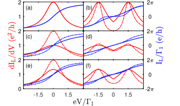
Figure 1: Conductances (red curves) and currents (blue curves) mediated by the MZMs in a two-lead setup with coupling rates $\Gamma_{1}$ and $\Gamma_{2}$. The coupling asymmetry is characterized by $\eta=\Gamma_{2}/\Gamma_{1}$, while the results for $\eta=0$, 1, and 0.5 are shown in (a) and (b), (c) and (d), and (e) and (f), respectively. In the left panels (a), (c) and (e), we consider $\epsilon_{M}=0$; while in the right panels (b), (d) and (f), we assume $\epsilon_{M}=1.5\Gamma_{1}$. In the whole plots, the solid curves display results from the modified BdG treatment, and the dashed curves from the standard BdG method Bee08 ; BCS-1 .

Importantly, in the result of Eq. (15), the CAR contribution ${\cal T}^{eh}_{12A}$ is nonzero even at the limit $\epsilon_{M}\to 0$. Also, since ${\cal T}^{eh}_{12A}={\cal T}^{ee}_{12}$ ($\Gamma^{e}_{\alpha}=\Gamma^{h}_{\alpha}$ under $\epsilon_{M}\to 0$), the teleportation channel is not closed even if the two MZMs ($\gamma_{1}$ and $\gamma_{2}$) have no coupling.

Local Conductance.— Let us consider first the simplest single-lead device where the probe lead is tunnel-coupled to the grounded Majorana wire from one side (e.g., the left side). We can use either the current formula based on the $S$ matrix or the formula based on the master equation, both giving the same results provided the modified BdG treatment is applied. Using Eq. (5), we may split the total current of Eq. (6) into two parts

$$I^{(1,2)}_{L}=\frac{e}{\hbar}\int^{\mu_{1}}_{\mu_{2}}d\omega\left(\frac{\Gamma^{e}_{1}\Gamma^{h}_{1}}{\Gamma^{e}_{1}+\Gamma^{h}_{1}}\right)\widetilde{\delta}(\omega\mp\epsilon_{M})\,.$$ (16)

Here we introduced $\mu_{1}=-\mu_{2}=eV$. The spectral function $\widetilde{\delta}(\omega\mp\epsilon_{M})$ takes the same form of Eq. (4), while for single-lead device the Lorentzian width is reduced to $\Gamma=(\Gamma^{e}_{1}+\Gamma^{h}_{1})/2$. Then, the differential conductance can be computed through

$$G=e\left(\frac{\partial I^{(1)}_{L}}{\partial\mu_{1}}+\frac{\partial I^{(2)}_{L}}{\partial\mu_{2}}\right)|_{\mu_{1}=eV,\,\mu_{2}=-eV}\,.$$ (17)

From Eqs. (16) and (17), we obtain the well-known Majorana conductance $G=\frac{e^{2}}{h}(1+1)=\frac{2e^{2}}{h}$, i.e., the quantized ZBP at $eV=\epsilon_{M}\to 0$ Law09 ; BNK11 ; Flen10 ; Flen16 ; Kou12 ; Kou19 , which holds also for the Majorana-induced resonant AR conductance at $eV=\epsilon_{M}\neq 0$ Law09 . We notice that, for the single-lead setup, both BdG treatments predict the same height of Majorana conductance peak, $2e^{2}/h$, as shown in Fig. 1(a) and (b), despite that the conventional BdG treatment predicts a narrower width of the conductance peak when $\epsilon_{M}\neq 0$.

Next, let us consider the two-lead device setup, which will reveal more remarkable differences between the two BdG treatments. Formally, the current formula is the same as Eq. (16), needing only by adding the CAR contribution such as $\Gamma^{e}_{1}\Gamma^{h}_{2}/(\Gamma^{e}_{1}+\Gamma^{h}_{2})$. Moreover, the Lorentzian width in $\widetilde{\delta}(\omega\mp\epsilon_{M})$ is now given by $\Gamma=(\Gamma^{e}_{1}+\Gamma^{h}_{1}+\Gamma^{e}_{2}+\Gamma^{h}_{2})/2$. In addition to increasing the resonance width, this more coupling to the right lead would decrease the heights of the various transmission coefficients, such as the LAR and CAR coefficients (${\cal T}^{eh}_{11A}$ and ${\cal T}^{eh}_{12A}$) as $\omega\to\epsilon_{M}$. We may term this type of consequences as a Majorana nonlocal-coupling-effect on the self energy. In particular, for symmetric coupling, the four coupling rates can be considered identical, and the heights of the the LAR and CAR peaks are reduced to 1/4, for either $\epsilon_{M}=0$ or not. At the limit $\epsilon_{M}\to 0$, owing to the complete “disconnection” between $\gamma_{1}$ and $\gamma_{2}$, the conventional BdG treatment predicts that ${\cal T}^{eh}_{12A}=0$ and ${\cal T}^{eh}_{11A}|_{\omega\to\epsilon_{M}}=1$, respectively. Then, the ZBP of the LAR conductance (in the left lead) would remain the same height as $2e^{2}/h$, being unaffected by the Majorana coupling to the opposite (right) lead. In contrast, based on either the modified BdG treatment or the MME, we predict the ZBP height as $G=\frac{2e^{2}}{h}\times\frac{1}{4}+\frac{e^{2}}{h}(\frac{1}{4}+\frac{1}{4})=e^{2}/h$. Here, the first part is from the LAR contribution, while the second part from the CAR process. In Fig. 1(c) and (d), we show the full results of this symmetric two-lead device, for both $\epsilon_{M}=0$ and $\epsilon_{M}\neq 0$. We find that the former case reveals greater difference between the two treatments. In Fig. 1(e) and (f), we also show the results for asymmetric coupling. Big difference exists as well in this case, particularly for $\epsilon_{M}\to 0$: the conventional BdG treatment predicts a constant ZBP of $2e^{2}/h$; while the modified BdG treatment predicts that the other side coupling will affect the height of the ZBP, e.g., for $\Gamma_{2}=\Gamma_{1}/2$, which is $1.5e^{2}/h$.

Teleportation Conductance.— Now we turn to the unequally biased two-lead device. For this setup ($\mu_{L}\neq\mu_{R}$), in addition to the AR process, the tunneling of electron between the two leads has contribution to the current. Again, applying Eq. (5), we obtain (at zero temperature)

$$I_{\alpha}=\frac{2e}{h}\Gamma_{\alpha}\left[\arctan(\frac{\mu_{\alpha}-\epsilon_{M}}{\Gamma})+\arctan(\frac{\mu_{\alpha}+\epsilon_{M}}{\Gamma})\right].$$ (18)

Here we have assumed the convention that $I_{1,2}=I_{L,R}$ and $\mu_{1,2}=\mu_{L,R}$. Rather than the total current, based on Eq. (5), simple analysis also allows us to know the individual components in $I^{(1)}_{L}$ and $I^{(2)}_{L}$, which result in

$$I_{L}=\frac{2e}{h}\int^{\mu_{L}}_{-\mu_{L}}d\omega\,{\cal T}^{eh}_{11A}(\omega)$$

$$~{}+\frac{e}{h}\left(\int^{\mu_{L}}_{-\mu_{R}}d\omega\,{\cal T}^{eh}_{12A}(\omega)+\int^{\mu_{R}}_{-\mu_{L}}d\omega\,{\cal T}^{eh}_{21A}(\omega)\right)$$

$$~{}+\frac{e}{h}\left(\int^{\mu_{L}}_{\mu_{R}}d\omega\,{\cal T}^{ee}_{12}(\omega)+\int^{-\mu_{R}}_{-\mu_{L}}d\omega\,{\cal T}^{hh}_{21}(\omega)\right).$$ (19)

The right-lead current $I_{R}$ can be similarly decomposed. Notice that, here, besides the contribution from the LAR (result of the first line) and CAR (result of the second line), the third line is the current from the left to the right lead through the teleportation channel. That is, the first term of the third line is from the electron-to-electron tunneling (from the left to the right lead), while the second term corresponds to an equivalent hole-to-hole tunneling (from the right to the left lead). In more detail, as an example, the second term of the third line was derived from $I^{(2)}_{L}(1h\leftarrow 2h)=\frac{e}{\hbar}(\widetilde{\Gamma}^{(+)}_{1}\widetilde{\Gamma}^{(-)}_{2}-\widetilde{\Gamma}^{(-)}_{1}\widetilde{\Gamma}^{(+)}_{2})/2\Gamma$, where “$2h$” stands for the hole in the right lead, and “$1h$” the hole in the left lead.

One can check that, based on the modified BdG $S$-matrix solution Eq. (Majorana Conductances in Three-Terminal Transports), the sum of all terms in Eq. (Majorana Conductances in Three-Terminal Transports) precisely recovers the result of Eq. (18). However, rather than the total current, below we are more interested in the current component through the teleportation channel, i.e., the third line of Eq. (Majorana Conductances in Three-Terminal Transports). For this purpose, we propose to extract this part of current via the consideration $\Delta I_{L}=I_{L}-\widetilde{I}_{L}$, where $\widetilde{I}_{L}$ denotes the sum of the AR currents (both LAR and CAR – the first and second lines of Eq. (Majorana Conductances in Three-Terminal Transports)), which flows back from the grounded superconductor to the left lead and can be measured as a branch circuit current. Then, from the third line of Eq. (Majorana Conductances in Three-Terminal Transports), we further obtain the differential conductance (termed as teleportation conductance in this work)

$$\Delta G_{LL}=\frac{d(\Delta I_{L})}{dV_{L}}=\frac{e^{2}}{h}\left[{\cal T}^{ee}_{12}(\mu_{L})+{\cal T}^{hh}_{21}(-\mu_{L})\right]\,.$$ (20)

Based on the $S$-matrix solution of the modified BdG treatment, Eq. (Majorana Conductances in Three-Terminal Transports), we have ${\cal T}^{ee}_{12}(\omega)=\Gamma^{e}_{1}\Gamma^{e}_{2}/|z|^{2}$ and ${\cal T}^{hh}_{21}(\omega)=\Gamma^{h}_{2}\Gamma^{h}_{1}/|z|^{2}$, where $|z|^{2}=(\omega-\epsilon_{M})^{2}+\Gamma^{2}$. To be more specific, we may assume the bias voltage as $\mu_{R}=0$ and $\mu_{L}=eV_{L}>0$. From the above result, it becomes clear that as $\epsilon_{M}\to 0$ the teleportation current $\Delta I_{L}$ and the differential conductance $\Delta G_{LL}$ are nonzero. This is a very important result, which indicates that, even at the limit $\epsilon_{M}\to 0$, the teleportation channel is still open.

Following Ref. BCS-1 as an example, which generalizes Ref. Bee08 by considering $\Gamma^{e}_{\alpha}\neq\Gamma^{h}_{\alpha}$ when $\epsilon_{M}\neq 0$, the conventional BdG treatment yields the solution of $S$ matrix which gives

$${\cal T}^{ee(hh)}_{12(21)}=|(\omega+i\Gamma)\xi\pm\epsilon_{M}\Gamma|^{2}/|z|^{2}\,,$$ (21)

where $|z|^{2}=(\omega^{2}-\epsilon^{2}_{M}-\Gamma^{2})^{2}+4\omega^{2}\Gamma^{2}$. Here we introduced $\xi=\Gamma^{e}-\Gamma^{h}$ and, for the sake of simplicity, assumed that $\Gamma^{e}_{1}=\Gamma^{e}_{2}\equiv\Gamma^{e}$, $\Gamma^{h}_{1}=\Gamma^{h}_{2}\equiv\Gamma^{h}$, and $\Gamma=\Gamma^{e}+\Gamma^{h}$. Substituting Eq. (21) into Eq. (20), we obtain

$$\Delta G_{LL}=(\frac{2e^{2}}{h})\,\frac{(\xi\mu_{L}+\epsilon_{M}\Gamma)^{2}+\xi^{2}\Gamma^{2}}{|z|^{2}}\,.$$ (22)

Here, in $|z|^{2}$, one should take $\omega=\mu_{L}$. We may emphasize that this result predicts that the teleportation channel vanishes when $\epsilon_{M}\to 0$. In this context, one may notice that $\xi_{\alpha}\equiv\Gamma^{e}_{\alpha}-\Gamma^{h}_{\alpha}=2\pi\nu|t_{\alpha}|^{2}(|u_{\alpha}|^{2}-|v_{\alpha}|^{2})$, which is closely related to the so-called local BCS charges BCS-1a ; BCS-1 ; BCS-2 , $q_{\alpha}=|u_{\alpha}|^{2}-|v_{\alpha}|^{2}$. Moreover, our numerical simulation based on the Kitaev lattice model Kita01 reveals that $q_{\alpha}/|u_{\alpha}|^{2}\propto\epsilon_{M}$, in the regime of relatively small Majorana coupling energies. Therefore, for the symmetric case $\xi_{1}=\xi_{2}=\xi$, we may denote $\xi/\Gamma=K\epsilon_{M}$ and reexpress the conductance under the conditions $V_{L}\to 0$ and $\epsilon_{M}\ll\Gamma$, as

$$\Delta G_{LL}=(\frac{2e^{2}}{h})\,(K^{2}+1/\Gamma^{2})\,\epsilon^{2}_{M}\,.$$ (23)

In Fig. 2, based on simulation of the Kitaev model for a spinless $p$-wave superconductor Kita01 , we display a logarithmic plot for this conductance as a function of $\epsilon_{M}$, to demonstrate the qualitative scaling behavior of $\Delta G_{LL}\propto\epsilon^{2}_{M}$, by noting that the prefactor $\widetilde{K}^{2}=K^{2}+1/\Gamma^{2}$ only depends on $\epsilon_{M}$ weakly. The weak dependence is originated from the coupling rate $\Gamma$ which decreases with increasing $\epsilon_{M}$, owing to the wavefunction extension of the Majorana bound states (towards the inner part of the quantum wire), while $K$ keeps almost a constant. Therefore, as a consequence of the approximate $\epsilon^{2}_{M}$-scaling behavior, the conventional BdG treatment predicts that the teleportation channel will be closed, when $\epsilon_{M}\to 0$. However, as shown by the blue-solid-line in Fig. 2, the modified BdG treatment predicts that the teleportation channel remains open even at the limit $\epsilon_{M}\to 0$, and the teleportation conductance $\Delta G_{LL}$ is almost independent of $\epsilon_{M}$.

Summary.— We have constructed a Majorana master equation which only associates with the BdG free occupation-number-states of the regular fermion. The results from the master equation approach forced us to modify the BdG treatment, in order to achieve consistent results. For the two-lead (three-terminal) transport setup, we revealed the existence of nonvanishing channels of teleportation and crossed Andreev reflections even if $\epsilon_{M}\to 0$. We also predicted different heights of the zero-bias-peak of the local conductance and different $\epsilon_{M}$-scaling behaviors of the teleportation conductance. Verification of the predictions by experiments will be of great interest.

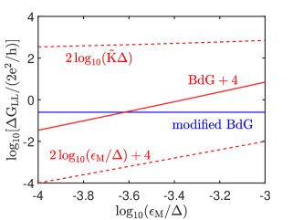
Figure 2: Scaling behavior of the teleportation conductance $\Delta G_{LL}$ with the Majorana coupling energy $\epsilon_{M}$, from simulation based on the Kitaev model Kita01 , $H_{M}=\sum^{N}_{j=1}[-\mu c^{\dagger}_{j}c_{j}-t(c^{\dagger}_{j}c_{j+1}+{\rm h.c.})+\Delta(c_{j}c_{j+1}+{\rm h.c.})]$, where $\mu$ is the chemical potential, $t$ is the hopping energy, and $\Delta$ is the superconducting order parameter. In numerical simulations, we set $t=\Delta=1.0$ and vary $\mu$ to realize the change of $\epsilon_{M}$, under the condition $\epsilon_{M}\ll\Gamma$ ($\Gamma$ is the coupling rate to the leads in the symmetric case as we assumed). We also consider the zero-bias limit $\mu_{L}\to 0$ while always setting $\mu_{R}=\epsilon_{F}=0$ ($\epsilon_{F}$ is the chemical potential of the superconductor). (i) The result shown by the blue-solid-line is from the modified BdG treatment, which reads as $\Delta G_{LL}=e^{2}/2h$ (in the symmetric coupling case). (ii) The result depicted by the red-solid line is from the conventional BdG treatment, which indicates an approximate scaling behavior of $\Delta G_{LL}\sim\epsilon^{2}_{M}$. Based on $\Delta G_{LL}=(\frac{2e^{2}}{h})\widetilde{K}^{2}\epsilon^{2}_{M}$, we also plot the two multiplying factors separately, by the red-dashed lines.

Acknowledgements.

— This work was supported by the National Key Research and Development Program of China (No. 2017YFA0303304) and the NNSF of China (Nos. 11675016, 11974011 & 61905174).

References

- (1) A.Y. Kitaev, Phys. Usp. 44, 131 (2001).
- (2) A. Y. Kitaev, Ann. Phys. (Amsterdam) 303, 2 (2003).
- (3) S. Das Sarma, M. Freedman, and C. Nayak, Quantum Inf. 1, 15001 (2015).
- (4) R. M. Lutchyn, J. D. Sau, and S. Das Sarma, Phys. Rev. Lett. 105, 077001 (2010).
- (5) Y. Oreg, G. Refael, and F. von Oppen, Phys. Rev. Lett. 105, 177002 (2010).
- (6) L. Fu and C. L. Kane, Phys. Rev. B 79, 161408 (2009).
- (7) J. Cayao, P. San-Jose, A. M. Black-Schaffer, R. Aguado, and E. Prada, Phys. Rev. B 96, 205425 (2017).
- (8) J. Cayao, A. M. Black-Schaffer, E. Prada, and R. Aguado, Beilstein J. Nanotechnol. 9, 1339 (2018).
- (9) J. Cayaoa and A. M. Black-Schaffer, Eur. Phys. J. Spec. Top. 227, 1387 (2018).
- (10) C.J. Bolech and E. Demler, Phys. Rev. Lett. 98, 237002 (2007).
- (11) J. Nilsson, A. R. Akhmerov, and C. W. J. Beenakker, Phys. Rev. Lett. 101, 120403 (2008).
- (12) B. Zocher and B. Rosenow, Phys. Rev. Lett. 111, 036802 (2013).
- (13) H. F. Lü, H. Z. Lu, and S. Q. Shen, Phys. Rev. B 86, 075318 (2012).
- (14) Y. S. Cao, P. Y. Wang, G. Xiong, M. Gong, and X. Q. Li, Phys. Rev. B 86, 115311 (2012).
- (15) K. T. Law, P. A. Lee, and T. K. Ng, Phys. Rev. Lett. 103, 237001 (2009).
- (16) M. Wimmer, A. R. Akhmerov, J. P. Dahlhaus, and C.W. J. Beenakker, New J. Phys. 13, 053016 (2011).
- (17) K. Sengupta, I. Zutic, H. J. Kwon, V. M. Yakovenko, and S. Das Sarma, Phys. Rev. B 63, 144531 (2001).
- (18) K. Flensberg, Phys. Rev. B 82, 180516(R) (2010).
- (19) E. B. Hansen, J. Danon, and K. Flensberg, Phys. Rev. B 93, 094501(R) (2016).
- (20) V. Mourik, K. Zuo, S. M. Frolov, S. R. Plissard, E. P. A. M. Bakkers, and L. P. Kouwenhoven, Science 336, 1003 (2012).
- (21) H. Zhang, D. E. Liu, M. Wimmer, and L. P. Kouwenhoven, Nat. Commun. 10, 5128 (2019).
- (22) B. van Heck, R. M. Lutchyn, and L. I. Glazman, Phys. Rev. B 93, 235431 (2016).
- (23) C. K. Chiu, J. D. Sau, and S. Das Sarma, Phys. Rev. B 96, 054504 (2017).
- (24) S. Vaitiekenas, M. T. Deng, J. Nygard, P. Krogstrup, and C. M. Marcus, Phys. Rev. Lett. 121, 037703 (2018).
- (25) S. Vaitiekenas, A. M. Whiticar, M. T. Deng, F. Krizek, J. E. Sestoft, C. J. Palmstrom, S. Marti-Sanchez, J. Arbiol, P. Krogstrup, L. Casparis, and C. M. Marcus, Phys. Rev. Lett. 121, 147701 (2018).
- (26) L. Hofstetter, S. Csonka, A. Baumgartner, G. Fülöp, S. d’Hollosy, J. Nygard, and C. Schönenberger, Phys. Rev. Lett. 107, 136801 (2011).
- (27) J. Gramich, A. Baumgartner, and C. Schönenberger, Phys. Rev. B 96, 195418 (2017).
- (28) E. B. Hansen, J. Danon,and K. Flensberg, Phys. Rev. B 97, 041411(R) (2018).
- (29) J. Danon, A. B. Hellenes, E. B. Hansen, L. Casparis, A. P. Higginbotham, and K. Flensberg, Phys. Rev. Lett. 124, 036801 (2020).
- (30) G. C. Ménard, G. L. R. Anselmetti, E. A. Martinez, D. Puglia, F. K. Malinowski, J. S. Lee, S. Choi, M. Pendharkar, C. J. Palmstrom, K. Flensberg, C. M. Marcus, L. Casparis, and A. P. Higginbotham, Phys. Rev. Lett. 124, 036802 (2020).
- (31) C. X. Liu, J. D. Sau, T. D. Stanescu, and S. Das Sarma, Phys. Rev. B 96, 075161 (2017).
- (32) E. Prada, R. Aguado, and P. San-Jose, Phys. Rev. B 96, 085418 (2017).
- (33) O. A. Awoga, J. Cayao, and A. M. Black-Schaffer, Phys. Rev. Lett. 123, 117001 (2019).
- (34) M. T. Deng, S. Vaitiekenas, E. Prada, P. San-Jose, J. Nygard, P. Krogstrup, R. Aguado, and C. M. Marcus, Phys. Rev. B 98, 085125 (2018).
- (35) E. Prada, P. San-Jose, M. W. A. de Moor, A. Geresdi, E. J. H. Lee, J. Klinovaja, D. Loss, J. Nygard, R. Aguado, and L. P. Kouwenhoven, From Andreev to Majorana bound states in hybrid superconductor-semiconductor nanowires, arXiv:1911.04512v2
- (36) J. Avila, F. Penaranda, E. Prada, P. San-Jose, and R. Aguado, Commun. Physics 2, 133 (2019).
- (37) P. San-Jose, J. Cayao, E. Prada, and R. Aguado, Sci. Rep. 6, 21427 (2016).
- (38) J. Cayao, E. Prada, P. San-Jose, and R. Aguado, Phys. Rev. B 91, 024514 (2015).
- (39) A. Vuik, B. Nijholt, A. R. Akhmerov, M. Wimmer, Reproducing topological properties with quasi-Majorana states, arXiv:1806.02801.
- (40) G. W. Semenoff and P. Sodano, Teleportation by a Majorana medium, arXiv:cond-mat/0601261; Stretching the electron as far as it will go, arXiv:cond-mat/0605147.
- (41) S. Tewari, C. Zhang, S. Das Sarma, C. Nayak, and D. H. Lee, Phys. Rev. Lett. 100, 027001 (2008).
- (42) L. Fu, Phys. Rev. Lett. 104, 056402 (2010).
- (43) X. Q. Li and L. Xu, Phys. Rev. B 101, 205401 (2020).
- (44) L. Qin, W. Feng, and X. Q. Li, Cross correlation mediated by distant Majorana zero modes with no overlap, arXiv:2104.12991v1; Chin. Phys. B (2021, in press)
- (45) W. Feng, L. Qin, and X. Q. Li, Cross correlation mediated by Majorana island with finite charging energy, arXiv:2108.12778
- (46) X. Q. Li, J. Y. Luo, Y. G. Yang, P. Cui, and Y. J. Yan, Phys. Rev. B 71, 205304 (2005).
- (47) J. S. Jin, J. Li, Y. Liu, X. Q. Li, and Y. J. Yan, J. Chem. Phys. 140, 244111 (2014).
- (48) I. Aleiner, P. Brouwer, and L. Glazman, Phys. Rep. 358, 309 (2002).