Community recovery in non-binary and temporal stochastic block models

Abstract

This article studies the estimation of latent community memberships from pairwise interactions in a network of $N$ nodes, where the observed interactions can be of arbitrary type, including binary, categorical, and vector-valued, and not excluding even more general objects such as time series or spatial point patterns. As a generative model for such data, we introduce a stochastic block model with a general measurable interaction space $\mathcal{S}$, for which we derive information-theoretic bounds for the minimum achievable error rate. These bounds yield sharp criteria for the existence of consistent and strongly consistent estimators in terms of data sparsity, statistical similarity between intra- and inter-block interaction distributions, and the shape and size of the interaction space. The general framework makes it possible to study temporal and multiplex networks with $\mathcal{S}=\{0,1\}^{T}$, in settings where both $N\to\infty$ and $T\to\infty$, and the temporal interaction patterns are correlated over time. For temporal Markov interactions, we derive sharp consistency thresholds. We also present fast online estimation algorithms which fully utilise the non-binary nature of the observed data. Numerical experiments on synthetic and real data show that these algorithms rapidly produce accurate estimates even for very sparse data arrays.

,
and

1 Introduction

Data sets in many application domains consist of non-binary pairwise interactions. Examples include human interactions in sociology and epidemiology [32, 35, 59], brain activity measurements in neuroscience [6], and financial interactions in economics [37]. Pair interactions are usually characterised by types (attributes, labels, features) of interacting objects (nodes, agents, individuals), and a set of objects with a common type is called a community (block, group, cluster). An important unsupervised learning problem is to infer the community memberships from the observed pair interactions, a task commonly known as community recovery or clustering [12].

Temporal interactions are an important particular case of non-binary interactions. The longitudinal nature of such data calls for replacing classical graph-based models by temporal and multiplex network models [20, 23, 26]. Although many powerful clustering methods exist for static networks (spectral methods [28], semidefinite programming [18], modularity maximisation [9], belief propagation [40], Bayesian methods [47], likelihood-based methods [53]), their extension to dynamic networks is not necessarily straightforward. In particular, simple approaches employing a static clustering method to a temporally aggregated network may lead to a severe loss of information [4], and they are in general ill-suited to online updating.

The stochastic block model (SBM), first explicitly defined in [22], has become a standard framework for analysing network data with binary interactions. The present article extends the definition of the stochastic block model to its most general form in which the observed interactions can be of arbitrary type, including binary, categorical, and vector-valued, and not excluding even more general objects such as time series or spatial point patterns. The observed data are represented by an $N$-by-$N$ symmetric array with entries in a general measurable space $\mathcal{S}$. The binary case with $\mathcal{S}=\{0,1\}$ corresponds to the most studied setting of random graphs. Temporal and multiplex networks can be represented by choosing $\mathcal{S}=\{0,1\}^{T}$ where $T$ equals the number of snapshots or layers. Other important choices for the interaction space include $\mathcal{S}=\{0,1\dots,L\}$ (link-labelled SBMs) and $\mathcal{S}=\mathbb{R}$ (weighted SBMs).

1.1 Related work

Existing works on community recovery in binary networks provide a strong information-theoretic foundation [14, 42, 58]. In particular, for $\mathcal{S}=\{0,1\}$ it is known that communities can be consistently recovered if the difference between intra- and inter-block link probabilities is large enough. Similar conclusions have been extended to models with categorical ($\mathcal{S}=\{0,\dots,L\}$) interactions [21, 25, 30, 55, 57] and real-valued ($\mathcal{S}=\mathbb{R}$) interactions [55]. In principle, temporal and multiplex network data with $\mathcal{S}=\{0,1\}^{T}$ could be modelled as categorical interactions with $2^{T}$ categories, but such approaches suffer from the following limitations. First, existing theoretical results are mainly limited to models with a bounded or slowly growing number of categories. For example, the results in [55] will directly apply only for $L=o(N)$. Second, algorithms designed for categorical interactions typically have complexity linear in $L$, and are hence inefficient even for a modest number of snapshots.

The present article is motivated by the inference of community structures from temporal network data; see [20] for a comprehensive review of dynamic network models. Earlier works on models, algorithms, and data experiments on temporal networks include [15, 33, 36, 48, 54, 56], where interactions are assumed temporally uncorrelated given the community memberships. Some of the aforementioned works also allow for time-varying community memberships. Because time-varying community memberships are known to involve model identifiability issues [36], this feature is left out of the scope of the present article. Information-theoretic studies on multiplex networks with independent layers include [19] presenting a strongly consistent estimator for models with $N=O(1)$ and $T\gg 1$, [45] establishing minimax error rates for models with $N,T\gg 1$ and balanced community sizes, [3] establishing posterior consistency in a Bayesian framework, and [7, 8, 27, 46, 49] presenting consistent estimators based on spectral clustering. Dynamic networks with temporally correlated interactions, or persistent edges, have so far attracted much less attention. Articles [5, 37] present numerical algorithms for estimating community memberships in temporally correlated SBMs in which the interaction patterns between nodes are positively correlated discrete-time Markov chains. Recently, [50, 51] presented EM algorithms for temporal SBMs where interactions are continuous-time Markov processes.

A detailed technical discussion of our contributions with respect to the most closely related earlier works is postponed to Section 6.

1.2 Main contributions

The main contributions of the present article can be summarised as follows:

1. We extend the SBM analysis to a general framework which allows the size and shape of the space of interactions $\mathcal{S}$ to vary with scale, making it possible to analyse vector-valued and functional interactions with dimension growing with scale, and multiplex and temporal networks where the number of layers or snapshots goes to infinity.

2. We derive a lower bound on the minimum achievable error rate of community recovery in a SBM with general interactions, including binary, categorical, weighted, and temporal patterns. This result extends in a natural but non-trivial way earlier results for binary and real-valued SBMs, by allowing the space of interactions $\mathcal{S}$ and the interaction distributions to be arbitrary. This is one of the first explicit quantitative lower bounds in this context.

3. We show that the maximum likelihood estimator recovers the true communities up to the information-theoretic lower bound. Combined with the lower bound, this yields sharp thresholds for community recovery in terms of the Rényi divergence between the interaction distributions. We also propose a polynomial-time algorithm which attains the desired lower bound under mild additional regularity assumptions.

4. We analyse temporal SBMs where interactions between nodes are correlated over time, and both the number of nodes $N$ and the number of time slots $T$ may tend to infinity. For sparse networks with Markov interactions, we derive information-theoretic consistency thresholds. The thresholds are presented in terms of an asymptotic formula for the Rényi divergence between two sparse Markov chains, which could be of independent interest.

5. We provide online algorithms for temporal networks in situations where the interaction parameters are known or unknown, with complexity linear in the number of layers $T$. In particular, a numerical study demonstrates that in a typical situation, we recover the correct communities starting from a blind random guess, even in very sparse regimes.

1.3 Outline

The rest of the article is structured as follows. Section 2 describes model details and notations. Section 3 summarises the main theoretical results for general non-binary network models, and Section 4 specialises to temporally correlated networks. Section 5 describes numerical experiments on synthetic and real data sets. Section 6 provides a technical discussion on our main contributions with respect to the state of the art. Finally, Section 7 describes avenues for future research. The proofs of the main theorems are presented in the appendices.

2 Model description and notations

2.1 General stochastic block model

The objective of study is a population of $N\geq 1$ mutually interacting nodes partitioned into $K\geq 2$ disjoint sets called blocks. The partition is represented by a node labelling $\sigma:[N]\to[K]$, so that $\sigma(i)$ indicates the block which contains node $i$. In line with the classical definition of a stochastic block model [22], we assume that interactions between node pairs can be of arbitrary type, and the set of possible interaction types is a measurable space $\mathcal{S}$. This general setup allows to model usual random graphs ($\mathcal{S}=\{0,1\}$), edge-labelled random graphs ($\mathcal{S}=\{0,\dots,L\}$, $\mathcal{S}=\mathbb{R}$), multilayer and temporal networks ($\mathcal{S}=\{0,1\}^{T}$, $\mathcal{S}=\{0,1\}^{\infty}$), and many other settings such as nodes interacting over a continuous time interval. In full generality, such a stochastic block model (SBM) is parameterised by a node labelling $\sigma:[N]\to[K]$ and an interaction kernel $(f_{k\ell})$ which is a collection of probability density functions with respect to a common sigma-finite reference measure $\mu$ on $\mathcal{S}$, such that $f_{k\ell}=f_{\ell k}$ for all $k,\ell=1,\dots,K$. These parameters specify a probability measure on a space of observations

$$\mathcal{X}\ =\ \Big{\{}x:[N]\times[N]\to\mathcal{S}:\ x_{ij}=x_{ji},\ x_{ii}=0\ \text{for all $i,j$}\Big{\}}$$

with probability density function

$$P_{\sigma}(x)\ =\prod_{1\leq i<j\leq N}f_{\sigma(i)\sigma(j)}\left(x_{ij}\right)$$ (2.1)

with respect to the $N(N-1)/2$-fold product of the reference measure $\mu$. Our main focus is on homogeneous models in which the interaction kernel can be represented as

$$f_{k\ell}\ =\ \begin{cases}f&\text{ if }k=\ell,\\ g&\text{ otherwise,}\end{cases}$$ (2.2)

for some probability densities $f$ and $g$ on $\mathcal{S}$, called the intra-block and inter-block interaction distribution, respectively. A homogeneous SBM is hence a probability density $P_{\sigma}$ on $\mathcal{X}$ specified by (2.1)–(2.2) and parameterised by a 5-tuple $(N,K,\sigma,f,g)$. For an observation $X$ distributed according to such $P_{\sigma}$, the entries $X_{ij}$, $1\leq i<j\leq N$, are mutually independent, and $X_{ij}$ is distributed according to $f$ when $\sigma(i)=\sigma(j)$, and according to $g$ otherwise.

The node labelling $\sigma$ representing the block membership structure is considered an unknown parameter to be estimated. When studying the average error rate of estimators, it is natural to regard the node labelling as a random variable distributed according to the uniform distribution $\pi(\sigma)=K^{-N}$ on parameter space $\mathcal{Z}=\big{\{}\sigma:[N]\to[K]\big{\}}.$ In this case the joint distribution of the node labelling and the observed data is characterised by a probability density

$$\mathbb{P}(\sigma,x)\ =\ \pi_{\sigma}P_{\sigma}(x)$$ (2.3)

on $\mathcal{Z}\times\mathcal{X}$ with respect to $\operatorname{card}_{\mathcal{Z}}\times\mu$, where $\operatorname{card}_{\mathcal{Z}}$ is the counting measure on $\mathcal{Z}$.

2.2 Classification error

The community recovery problem is the task of developing an algorithm $\phi:\mathcal{X}\to\mathcal{Z}$ which maps an observed data array $X=(X_{ij})$ into an estimated node labelling $\hat{\sigma}=\phi(X)$. Stated like this, the recovery problem is ill-posed because the map $\sigma\mapsto P_{\sigma}$ defined by (2.1) is in general non-injective. Therefore, we adopt the common approach in which the goal is to recover the unlabelled block structure, that is, the partition $[\sigma]=\{\sigma^{-1}(k):k\in[K]\}$, and the estimation error is considered small when $[\hat{\sigma}]$ is close to $[\sigma]$. Accordingly, we define for node labellings $\sigma_{1},\sigma_{2}:[N]\to[K]$ an error quantity by

$$\operatorname{Ham}^{*}(\sigma_{1},\sigma_{2})\ =\ \min_{\rho\in\operatorname{Sym}(K)}\operatorname{Ham}(\rho\circ\sigma_{1},\sigma_{2})$$

where $\operatorname{Sym}(K)$ denotes the group of permutations on $[K]$ and $\operatorname{Ham}$ refers to the Hamming distance. The above error takes values in $\{0,\dots,N\}$ and depends on its inputs only via the partitions $[\sigma_{1}]$ and $[\sigma_{2}]$. The normalised error quantity $N^{-1}\operatorname{Ham}^{*}(\sigma_{1},\sigma_{2})$ is known as the classification error [12, 38].

When analysing the average performance of an estimator, we can view $\hat{\sigma}$ as a $\mathcal{Z}$-valued random variable defined on the observation space $\mathcal{X}$. Then $E_{\sigma}\operatorname{Ham}^{*}(\hat{\sigma},\sigma)$ equals the expected clustering error given a true parameter $\sigma$, and

$$\mathbb{E}\operatorname{Ham}^{*}(\hat{\sigma})\ =\ \sum_{\sigma\in\mathcal{Z}}\pi_{\sigma}E_{\sigma}\operatorname{Ham}^{*}(\hat{\sigma},\sigma)$$

is the average clustering error with respect to the uniform distribution $\pi_{\sigma}=K^{-N}$ on the parameter space.

2.3 Consistent estimators

A large-scale network is represented as a sequence of models $P_{\sigma}^{(\eta)}$ indexed by a scale parameter $\eta=1,2,\dots$ In this setting the model dimensions $N^{(\eta)},K^{(\eta)}$, the node labelling $\sigma^{(\eta)}$, the interaction densities $f^{(\eta)},g^{(\eta)}$, as well as the spaces $\mathcal{S}^{(\eta)},\mathcal{X}^{(\eta)},\mathcal{Z}^{(\eta)}$ all depend on the scale parameter $\eta$. In this setup, an estimator is viewed as a map $\phi^{(\eta)}:\mathcal{X}^{(n)}\to\mathcal{Z}^{(\eta)}$. For nonnegative sequences $a=a^{(\eta)}$ and $b=b^{(\eta)}$ we denote $a=o(b)$ when $\limsup_{\eta\to\infty}a^{(\eta)}/b^{(\eta)}=0$, and $a=O(b)$ when $\limsup_{\eta\to\infty}a^{(\eta)}/b^{(\eta)}<\infty$. We write $a=\omega(b)$ when $b=o(a)$, $a=\Omega(b)$ when $b=O(a)$, and $a=\Theta(b)$ when $a=O(b)$ and $b=O(a)$. We also denote $a\ll b$ for $a=o(b)$, $a\lesssim b$ for $a=O(b)$, $a\asymp b$ for $a=\Theta(b)$, and $a\sim b$ for $a=(1+o(1)b$. To avoid overburdening the notation, the scale parameter is mostly omitted from the notation in what follows.

For a large-scale model with $N\gg 1$ nodes, an estimator $\hat{\sigma}=\hat{\sigma}^{(\eta)}$ is called consistent if $\mathbb{E}\operatorname{Ham}^{*}(\hat{\sigma})=o(N)$, and strongly consistent if $\mathbb{E}\operatorname{Ham}^{*}(\hat{\sigma})=o(1)$. A strongly consistent estimator is also said to achieve exact recovery, and a consistent estimator is said to achieve almost exact recovery [1].

2.4 Information-theoretic divergences and distances

Let us recall basic information divergences and distances associated with probability distributions $f$ and $g$ on a general measurable space $\mathcal{S}$ [16, 52]. The Rényi divergence of positive order $\alpha\not=1$ is defined as

$$D_{\alpha}(f\|g)=(\alpha-1)^{-1}\log\int\left(\frac{df}{d\mu}\right)^{\alpha}\left(\frac{dg}{d\mu}\right)^{1-\alpha}d\mu,$$

where $\mu$ is an arbitrary measure which dominates $f$ and $g$. We use the conventions $\log 0=-\infty$, $0/0=0$ and $x/0=\infty$ for $x>0$. In particular, if $f\not\perp g$ and $\alpha<1$, then $D_{\alpha}(f\|g)<\infty$. In the symmetric case with $\alpha=\frac{1}{2}$ we write

$$D_{1/2}(f,g)\ =\ -2\log\int\sqrt{\frac{df}{d\mu}}\sqrt{\frac{dg}{d\mu}}d\mu,$$

and note that this quantity is related to the Hellinger distance defined by

$$\mathrm{Hel}^{2}(f,g)\ =\ \frac{1}{2}\int\left(\sqrt{\frac{df}{d\mu}}-\sqrt{\frac{dg}{d\mu}}\right)^{2}d\mu,$$

via the formula $D_{1/2}(f,g)=-2\log\left(1-\mathrm{Hel}^{2}(f,g)\right)$. In what follows, we assume that a sigma-finite reference measure $\mu$ on $\mathcal{S}$ is fixed once and for all, and we write $\frac{df}{d\mu},\frac{dg}{d\mu}$ simply as $f,g$, and we omit $d\mu$ from the integral signs, so that $D_{\alpha}(f\|g)=(\alpha-1)^{-1}\log\int f^{\alpha}g^{1-\alpha}$. When $\mathcal{S}$ is countable, $\mu$ is always chosen as the counting measure, in which case write $D_{\alpha}(f\|g)=(\alpha-1)^{-1}\log\sum_{x\in\mathcal{S}}f^{\alpha}(x)g^{1-\alpha}(x)$, and so on. We also denote symmetrised Rényi divergences by $D^{s}_{\alpha}(f,g)=\frac{1}{2}(D_{\alpha}(f\|g)+D_{\alpha}(g\|f))$.

3 Results for general SBMs

Section 3.1 describes information-theoretic thresholds for consistent community recovery. Section 3.2 specialises to sparse networks. Section 3.3 describes a polynomial-time algorithm and discusses its accuracy.

3.1 General information thresholds

The following theorem characterises fundamental information-theoretic limits for the recovery of block memberships from data generated by a homogeneous $\mathcal{S}$-valued SBM. It does not make any scaling assumptions on the model dimensions $N$ and $K$, or on the space of interaction types $\mathcal{S}$, and its proof indicates that maximum likelihood estimators achieve the upper bound.

Theorem 3.1.

For a homogeneous SBM with $N$ nodes, $K$ blocks, and interaction distributions $f,g$ on a general measurable space $\mathcal{S}$ having Rényi divergence $I=D_{1/2}(f,g)$, the minimum average classification error among all estimators $\hat{\sigma}:\mathcal{X}\to\mathcal{Z}$ is bounded from below by

$$\min_{\hat{\sigma}}\mathbb{E}\left(\frac{\operatorname{Ham}^{*}(\hat{\sigma})}{N}\right)\ \geq\ \frac{1}{84}K^{-3}e^{-\frac{N}{K}I-\sqrt{8NI_{21}}}-\frac{1}{6}e^{-\frac{N}{8K}}$$

and from above by

$$\min_{\hat{\sigma}}\mathbb{E}\left(\frac{\operatorname{Ham}^{*}(\hat{\sigma})}{N}\right)\ \leq\ 8e(K-1)e^{-(1-\zeta-\kappa)\frac{N}{K}I}+K^{N}e^{-\frac{1}{4}(\frac{\zeta}{K-1}-\epsilon)(N/K)^{2}I}+2Ke^{-\frac{1}{3}\epsilon^{2}\frac{N}{K}},$$

for all $0\leq\epsilon\leq\zeta\leq\frac{1}{21}$, where $\kappa=56\max\{K^{2}e^{-\frac{NI}{8K}},\,KN^{-1}\}$ and another auxiliary parameter is defined by $I_{21}=\left(\frac{1}{2}-K^{-1}\right)K^{-1}I+\frac{1}{2}K^{-1}J$ with $J=\left(\int\sqrt{fg}\right)^{-1}\int\sqrt{fg}\log^{2}\frac{f}{g}$.

Proof.

The lower bound is established in Proposition C.13 in Appendix C, while the upper bound is analysed in Appendix D and follows from Proposition D.3. ∎

The next key result characterises information-theoretic recovery conditions in large-scale networks, for which we emphasise that the model dimensions $N=N^{(\eta)}$ and $K=K^{(\eta)}$, the interaction distributions $f=f^{(\eta)}$ and $g=g^{(\eta)}$, and also the interaction type space $\mathcal{S}=\mathcal{S}^{(\eta)}$, are allowed to depend on a scale parameter $\eta$ which omitted from notation for clarity.

Theorem 3.2.

For a homogeneous SBM with $N\gg 1$ nodes, $K\asymp 1$ blocks, and interaction distributions $f$ and $g$ having Rényi divergence $I=D_{1/2}(f,g)$:

1. a consistent estimator exists if $I\gg N^{-1}$, and does not exist if $I\lesssim N^{-1}$;

2. a strongly consistent estimator exists if $I\geq(1+\Omega(1))\frac{K\log N}{N}$, and does not exist if $I\leq(1-\Omega(1))\frac{K\log N}{N}$.

Furthermore, if $N^{-1}\ll I\ll 1$ and $K\asymp 1$, the optimal achievable misclassification rate equals

$$\min_{\hat{\sigma}}\mathbb{E}\left(\frac{\operatorname{Ham}^{*}(\hat{\sigma})}{N}\right)\ \asymp\ e^{-(1-o(1))NI/K}.$$ (3.1)

Proof.

The nonexistence statements are a direct consequence of the lower bound in Theorem 3.1 combined with Lemma C.12 to guarantee that $J\lesssim I$. The existence results follow by analysing the upper bound of Theorem 3.1, which is done in Proposition D.4 in Appendix D. Formula (3.1) follows from the bounds of Theorem 3.1 by choosing $\zeta=(NI)^{-1/2}$ and $\epsilon=\frac{1}{2}\frac{\zeta}{K-1}$, and recalling $J\lesssim I$ by Lemma C.12. ∎

The following examples illustrate how Theorem 3.2 can be applied to various types of SBMs in sparse and dense regimes.

Example 3.3 (Binary interactions).

A graph in which two nodes in the same community (resp. different communities) are linked with probability $p$ (resp. $q$) forms an instance of a homogeneous SBM where the $\frac{1}{2}$-order Rényi divergence between Bernoulli interaction distributions equals $I=-2\log((1-p)^{1/2}(1-q)^{1/2}+p^{1/2}q^{1/2})$. In a sparse regime where $p=p_{0}\frac{\log N}{N}$ and $q=q_{0}\frac{\log N}{N}$ for scale-independent constants $p_{0},q_{0}>0$, this is approximated by $I\sim(\sqrt{p_{0}}-\sqrt{q_{0}})^{2}\frac{\log N}{N}$. Theorem 3.2 tells that a strongly consistent estimator exists if $(\sqrt{p_{0}}-\sqrt{q_{0}})^{2}>K$ and does not if $(\sqrt{p_{0}}-\sqrt{q_{0}})^{2}<K$. This is the well-known threshold for strong consistency in sparse binary SBMs [2, 42]. Alternatively, in a dense regime where $p=p_{0}+\epsilon$ and $q=p_{0}$ for $\epsilon=o(1)$ and some scale-independent constant $0<p_{0}<1$, we find that $I\sim\frac{\epsilon^{2}}{4p_{0}(1-p_{0})}$. Especially, when $\epsilon=c(\frac{\log N}{N})^{1/2}$ for some scale-independent constant $c>0$, then we find that a strongly consistent estimator exists if $(p_{0}-\frac{1}{2})^{2}>\frac{1-c^{2}/K}{4}$ and does not if $(p_{0}-\frac{1}{2})^{2}<\frac{1-c^{2}/K}{4}$.

Example 3.4 (Poisson interactions).

Consider an integer-valued SBM where the interaction between two nodes in the same block (resp. different blocks) is a Poisson-distributed random integer with mean $\lambda$ (resp. $\mu$). The $\frac{1}{2}$-order Rényi divergence between such Poisson distributions equals $I=(\sqrt{\lambda}-\sqrt{\mu})^{2}$. In a sparse regime where $\lambda=\lambda_{0}\frac{\log N}{N}$ and $\mu=\mu_{0}\frac{\log N}{N}$ for scale-independent constants $\lambda_{0},\mu_{0}>0$, Theorem 3.2 tells that a strongly consistent estimator exists if $(\sqrt{\lambda_{0}}-\sqrt{\mu_{0}})^{2}>K$ and does not if $(\sqrt{\lambda_{0}}-\sqrt{\mu_{0}})^{2}<K$. In a dense regime where $\lambda=\lambda_{0}+\epsilon$ and $\mu=\lambda_{0}$ for $\epsilon=o(1)$ and some scale-independent constant $\lambda_{0}>0$, we see that $I\sim\frac{\epsilon^{2}}{4\lambda_{0}}$. Especially, if $\epsilon=c(\frac{\log N}{N})^{1/2}$ for some scale-independent constant $c>0$, then a strongly consistent estimator exists when $\frac{c^{2}}{4\lambda_{0}}>K$ and does not when $\frac{c^{2}}{4\lambda_{0}}<K$.

Example 3.5 (Normal interactions).

Consider a real-valued SBM where the interaction between two nodes in the same block (resp. different blocks) follows a normal distribution with mean zero and standard deviation $\sigma$ (resp. $\tau$). The $\frac{1}{2}$-order Rényi divergence between such normal distributions equals $I=\log(1+\frac{(\sigma-\tau)^{2}}{2\sigma\tau})$. Theorem 3.2 combined with Taylor’s approximation $\log(1+t)=t+O(t^{2})$ tells that a consistent estimator exists if $\frac{(\sigma-\tau)^{2}}{2\sigma\tau}\gg N^{-1}$ and does not if $\frac{(\sigma-\tau)^{2}}{2\sigma\tau}\lesssim N^{-1}$; and that a strongly consistent estimator exists if $\frac{(\sigma-\tau)^{2}}{2\sigma\tau}\geq(1+\Omega(1))K\frac{\log N}{N}$ and does not if $\frac{(\sigma-\tau)^{2}}{2\sigma\tau}\leq(1-\Omega(1))K\frac{\log N}{N}$.

Example 3.6 (Multiplex networks).

An SBM with product-form intra- and inter-block interaction distributions $f=\prod_{t=1}^{T}f_{t}$ and $g=\prod_{t=1}^{T}g_{t}$ on $\mathcal{S}=\mathcal{S}_{1}\times\cdots\times\mathcal{S}_{T}$ corresponds to observing $T$ mutually independent network layers over a common node set, where data on the $t$-th layer are distributed according to an SBM with interaction distributions $f_{t}$ and $g_{t}$ on $\mathcal{S}_{t}$. By observing that $I=\sum_{t=1}^{T}I_{t}$ for $I=D_{1/2}(f,g)$ and $I_{t}=D_{1/2}(f_{t},g_{t})$, Theorem 3.2 tells that strong consistency is possible when $\sum_{t=1}^{T}I_{t}\geq(1+\Omega(1))\frac{K\log N}{N},$ and impossible when $\sum_{t=1}^{T}I_{t}\leq(1-\Omega(1))\frac{K\log N}{N}.$ Similarly, consistency is possible when $\sum_{t=1}^{T}I_{t}\gg N^{-1}$ and impossible when $\sum_{t=1}^{T}I_{t}\lesssim N^{-1}$. In the binary case where $\mathcal{S}_{t}=\{0,1\}$ for all $t$, corresponding thresholds have been derived in [3, 45]. The present example is an important extension allowing to analyse heterogeneous multiplex networks in which some layers may only be partially observed (cf. Example 3.9) and some may carry real-valued edge labels (cf. Example 3.12).

3.2 Sparse networks

Sparse networks can be modelled using intra-block and inter-block interaction distributions of form

$$f\ =\ (1-p_{0}\rho)\delta_{0}+p_{0}\rho\tilde{f}\qquad\text{and}\qquad g\ =\ (1-q_{0}\rho)\delta_{0}+q_{0}\rho\tilde{g},$$ (3.2)

where $\delta_{0}$ is the Dirac measure at an element $0\in\mathcal{S}$ representing no-interaction, probability measures $\tilde{f},\tilde{g}$ on $\mathcal{S}\setminus\{0\}$ are conditional distributions of interaction types given that there is an interaction, $p_{0},q_{0}>0$ are scale-independent constants, and $\rho\ll 1$ describes the overall network density. The following result describes how the regimes for consistent and strongly consistent community recovery are characterised by a fundamental information quantity

$$\tilde{I}\ =\ \left(\sqrt{p_{0}}-\sqrt{q_{0}}\right)^{2}+2\sqrt{p_{0}q_{0}}\,\mathrm{Hel}^{2}(\tilde{f},\tilde{g}).$$ (3.3)

In the above formula, the quantity $\left(\sqrt{p_{0}}-\sqrt{q_{0}}\right)^{2}$ corresponds to information gained from observing whether or not there is an interaction, and the Hellinger distance $\mathrm{Hel}(\tilde{f},\tilde{g})$ characterises the additional information gained by observing the types of interactions between node pairs.

Theorem 3.7.

For a homogeneous SBM with $N\gg 1$ nodes, $K\asymp 1$ blocks, and interaction distributions of form (3.2) where $\rho\ll 1$, and $p_{0},q_{0}$ are scale-independent constants:

1. a consistent estimator exists if $\rho\tilde{I}\gg N^{-1}$, and does not exist if $\rho\tilde{I}\lesssim N^{-1}$;

2. a strongly consistent estimator exists if $\rho\tilde{I}\geq(1+\Omega(1))\frac{K\log N}{N}$, and does not exist if $\rho\tilde{I}\leq(1-\Omega(1))\frac{K\log N}{N}$;

Proof.

Taylor’s approximations show that the Rényi divergence of order $\alpha\neq 1$ for probability distributions of form (3.2) is approximated by

$$D_{\alpha}(f\|g)\ =\ \frac{p^{\alpha}q^{1-\alpha}}{\alpha-1}e^{(\alpha-1)D_{\alpha}(\tilde{f}\|\tilde{g})}-\frac{\alpha p+(1-\alpha)q}{\alpha-1}+O(\rho^{2}),$$ (3.4)

where $p=p_{0}\rho$ and $q=q_{0}\rho$. In particular, the formula $1-\mathrm{Hel}(\tilde{f},\tilde{g})^{2}=e^{-\frac{1}{2}D_{1/2}(\tilde{f},\tilde{g})}$ implies that the Rényi divergence of order half is given by

$$D_{1/2}(f,g)\ =\ (\sqrt{p}-\sqrt{q})^{2}+2\sqrt{pq}\,\mathrm{Hel}^{2}(\tilde{f},\tilde{g})+O(\rho^{2}),$$ (3.5)

so that $D_{1/2}(f,g)=(1+o(1))\rho\tilde{I}$. Statements (i) and (ii) hence follow from Theorem 3.2. ∎

The following three examples illustrate the applicability of Theorem 3.7 for finite and real-valued interaction spaces.

Example 3.8 (Sparse categorical interactions).

Consider a categorical stochastic block model with intra- and inter-block interactions distributed according to (3.2) in which $\tilde{f}$ and $\tilde{g}$ are probability distributions on $\{1,\dots,L\}$. The critical information quantity defined in (3.3) can then be written as

$$\tilde{I}\ =\ \left(\sqrt{p_{0}}-\sqrt{q_{0}}\right)^{2}+\sqrt{p_{0}q_{0}}\sum_{\ell=1}^{L}\left(\sqrt{\tilde{f}(\ell)}-\sqrt{\tilde{g}(\ell)}\right)^{2}.$$

This model was studied in [25] in a parameter regime with $\rho=\frac{\log N/K}{N/K}\asymp K\frac{\log N}{N}$, where it was assumed that neither $L$ nor the probabilities $\tilde{f}(\ell)$, $\tilde{g}(\ell)>0$ depend on the scale parameter. In this case $\tilde{I}$ is a scale-independent constant, and by applying Theorem 3.7:(ii) we recover the main results of [25] stating that a strongly consistent estimator exists if $\tilde{I}>1$ and does not exist if $\tilde{I}<1$. Unlike [25], Theorem 3.7 does not require any regularity conditions on $\tilde{f}$ and $\tilde{g}$.

Example 3.9 (Censored binary SBM).

Assume that between any pair of nodes in the same community (resp. different communities), there is an edge with probability $a$ (resp. $b$) and the edge status of the node pair is observed with probability $p=p_{0}\rho$ (resp. $q=q_{0}\rho$) regardless of whether an edge is present or not. We assume that $\rho\ll 1$, and that $a,b,p_{0},q_{0}$ are scale-independent constants. The observed data can be modelled as an instance of (3.2) with interaction type space $\mathcal{S}=\{0,10,11\}$ where 0 = censored, 10 = observed&absent, and 11 = observed&present, and

$$\tilde{f}(10) =1-a, \qquad\qquad\tilde{g}(10) =1-b,$$

$$\tilde{f}(11) =a, \qquad\qquad\tilde{g}(11) =b.$$

The fundamental information quantity in (3.3) equals $\tilde{I}=\left(\sqrt{p_{0}}-\sqrt{q_{0}}\right)^{2}+2\sqrt{p_{0}q_{0}}\,\mathrm{Hel}^{2}(\tilde{f},\tilde{g}),$ where $\mathrm{Hel}(\tilde{f},\tilde{g})^{2}=\frac{1}{2}(\sqrt{1-a}-\sqrt{1-b})^{2}+\frac{1}{2}(\sqrt{a}-\sqrt{b})^{2}.$ Assume that $t=p_{0}=q_{0}$ equals a common observation rate and $\rho=\frac{\log N}{N}$. Theorem 3.7 then tells that exact recovery is possible if $t>t_{\rm crit}$ and impossible if $t<t_{\rm crit}$. where $t_{\rm crit}=\frac{K}{2\mathrm{Hel}^{2}(\tilde{f},\tilde{g})}$. For $K=2$, this coincides with the exact recovery threshold recently presented in Dhara et al. [11], and extends their criterion into models with $K>2$ and $p_{0}\neq q_{0}$.

Example 3.10 (Censored real-valued SBM).

Assume that associated to each pair of nodes in the same community (resp. different communities), there is a random variable following a normal distribution with mean zero and standard deviation $\sigma$ (resp. $\tau$), and this variable is observed with probability $p=p_{0}\rho$ (resp. $q=q_{0}\rho$), where $\rho\ll 1$ and $\sigma,\tau,p_{0},q_{0}>0$ are scale-independent constants. The observed data can be modelled as an instance of (3.2) with interaction type space $\mathcal{S}=\mathbb{R}$ in which $\tilde{f}=\operatorname{Nor}(0,\sigma^{2})$ and $\tilde{g}=\operatorname{Nor}(0,\tau^{2})$, and the value 0 represents no-observation. The fundamental information quantity in (3.3) then equals

$$\tilde{I}\ =\ \left(\sqrt{p_{0}}-\sqrt{q_{0}}\right)^{2}+2\sqrt{p_{0}q_{0}}\,\left(1-\sqrt{\frac{2\sigma\tau}{\sigma^{2}+\tau^{2}}}\right).$$

If $t=p_{0}=q_{0}$ equals a common observation rate and $\rho=\frac{\log N}{N}$, then Theorem 3.7 then tells that exact recovery is possible if $t>t_{\rm crit}$ and impossible if $t<t_{\rm crit}$ were $t_{\rm crit}=\frac{K/2}{1-\sqrt{\frac{2\sigma\tau}{\sigma^{2}+\tau^{2}}}}$.

3.3 Polynomial-time algorithm

To cluster non-binary SBMs in a polynomial time in $N$, we propose Algorithm 1 which employs spectral clustering as a subroutine to produce a moderately accurate initial clustering, and then performs a refinement step through node-wise likelihood maximisation. Similarly to [14, 55], for technical reasons related to the proofs, the initialisation step of Algorithm 1 involves $N$ separate spectral clustering steps. A consensus step is therefore needed at the end, to correctly permute the individual predictions. Numerical experiments indicate that in practice it often suffices to do one spectral clustering on a binary matrix, and remove this consensus step. We will discuss practical aspects in more detail in Section 5.

Input: $\mathcal{S}$-valued interaction array $X_{ij}$; interaction distributions $f,g$; set $\mathcal{A}\subset\mathcal{S}$.

Output: Estimated node labelling $\hat{\sigma}$.

Step 1: Coarse clustering using binary interaction data Compute a binary matrix $\tilde{X}$ by setting $\tilde{X}_{ij}=1(X_{ij}\not\in\mathcal{A})$.

for $i=1,\dots,N$ do

       Let $\tilde{X}_{-i}$ be the submatrix of $\tilde{X}$ with row $i$ and column $i$ removed.

       Compute a node labelling $\tilde{\sigma}_{i}$ on $[N]\setminus\{i\}$ by applying a standard graph clustering algorithm with adjacency matrix $\tilde{X}_{-i}$.

Step 2: Refined clustering using full interaction data for $i=1,\dots,N$ do

       Compute $h_{i}(k)=\sum_{j:\tilde{\sigma}_{i}(j)=k}\log\frac{f(X_{ij})}{g(X_{ij})}$ for all $k\in[K]$.

       Set $\hat{\sigma}_{i}(i)=\operatorname*{arg\,max}_{k\in[K]}h_{i}(k)$ with arbitrary tie breaks.

       Set $\hat{\sigma}_{i}(j)=\tilde{\sigma}_{i}(j)$ for $j\neq i$.

Step 3: Consensus Select $\hat{\sigma}_{1}$ as a baseline node labelling and set $\hat{\sigma}(1)=\hat{\sigma}_{1}(1)$.

for $i=2,\dots,N$ do

       Set $\hat{\sigma}(i)=\operatorname*{arg\,max}_{\ell}{\lvert\hat{\sigma}_{i}^{-1}(\hat{\sigma}_{i}(i))\cap\hat{\sigma}_{1}^{-1}(\ell)\rvert}$ with arbitrary tie breaks.

Algorithm 1 Clustering using general $\mathcal{S}$-valued interaction data

The following theorem characterises the accuracy of Algorithm 1 for large-scale models, and implies that under mild technical conditions this algorithm achieves the optimal error rate in Theorem 3.2. The proof of Theorem 3.11 is given in Appendix E.

Theorem 3.11.

Consider a homogeneous SBM with $N\gg 1$ nodes, $K\asymp 1$ blocks, and interaction distributions $f$ and $g$ having Rényi divergence $I=D_{1/2}(f,g)$. If $(f(\mathcal{A})^{1/2}-g(\mathcal{A})^{1/2})^{2}\gg N^{-1}\frac{D_{1+r}^{s}(f,g)}{D_{r}^{s}(f,g)}$ for some $0<r\leq\frac{1}{2}$, then the classification error of Algorithm 1 applied with $\mathcal{A}\subset\mathcal{S}$ is bounded by

$$\mathbb{E}\left(\frac{\operatorname{Ham}^{*}(\hat{\sigma})}{N}\right)\ \leq\ Ke^{-(1-o(1))2r\frac{N}{K}I}+o(1).$$

The following three examples illustrate how Theorem 3.11 can be applied to analyse the performance of Algorithm 1 in sparse and dense settings.

Example 3.12 (Normal interactions).

Consider the real-valued SBM in Example 3.5 with intra- and inter-block interaction distributions $f=\operatorname{Nor}(0,\sigma^{2})$ and $g=\operatorname{Nor}(0,\tau^{2})$. Assume that $\sigma>0$ is scale-independent and $\tau=\sigma(1+\epsilon)$ for some $\epsilon=o(1)$. Then the $\frac{1}{2}$-order Rényi divergence equals $I\sim\frac{1}{2}\epsilon^{2}$, and the symmetrised $\frac{3}{2}$-order Rényi divergence is finite and approximated by $D_{3/2}^{s}(f,g)\sim\frac{3}{2}\epsilon^{2}$. For an interval $\mathcal{A}=[-x,x]$ we find that $f(\mathcal{A})-g(\mathcal{A})=2(\Phi(\frac{x}{\sigma})-\Phi(\frac{x}{\tau}))=2\frac{x}{\sigma}\Phi^{\prime}(\frac{x}{\sigma})\epsilon+O(\epsilon^{2})$, where $\Phi$ is the standard normal cdf. Thus, $(\sqrt{f(\mathcal{A})}-\sqrt{g(\mathcal{A})})^{2}\asymp\epsilon^{2}$ for any $x=O(1)$. Theorem 3.11 hence tells that Algorithm 1 applied with $\mathcal{A}=[-1,1]$ is consistent if $\epsilon^{2}\gg N^{-1}$ and strongly consistent if $\frac{1}{2}\epsilon^{2}\geq(1+\Omega(1))\frac{K\log N}{N}$. In light of Example 3.5, we see that Algorithm 1 recovers communities up to the information-theoretic boundaries in Theorem 3.2.

Example 3.13 (Geometric interactions).

Suppose $f=\operatorname{Geo}(a)$ and $g=\operatorname{Geo}(a+\epsilon)$ with $a$ scale-independent and $\epsilon\ll 1$. Then the $\frac{1}{2}$-order Rényi divergence is $I\sim\frac{\epsilon^{2}}{4a(1-a)^{2}}$. Theorem 3.2 tells that a consistent estimator exists if $\epsilon\gg N^{-1/2}$ and a strongly consistent estimator exists if $\frac{\epsilon^{2}}{a(1-a)^{2}}\geq(1+\Omega(1))\frac{K\log N}{N}$. We also note that $(\sqrt{f(0)}-\sqrt{g(0)})^{2}\asymp\epsilon^{2}$, and that the symmetrised $\frac{3}{2}$-order Rényi divergence is finite and satisfies $D^{s}_{3/2}(f,g)\asymp\epsilon^{2}$. Theorem 3.11 hence tells that Algorithm 1 applied with $\mathcal{A}=\{0\}$ recovers the communities up to the information-theoretic boundaries in Theorem 3.2.

Example 3.14 (Zero-inflated geometric distributions).

Consider an integer-valued stochastic block model with intra- and inter-block interactions distributed according to

$$f(x)=\begin{cases}1-\rho p_{0},&\quad x=0,\\ \rho p_{0}(1-a)a^{x},&\quad x\geq 1,\end{cases}\qquad\text{and}\qquad g(x)=\begin{cases}1-\rho q_{0},&\quad x=0,\\ \rho q_{0}(1-b)b^{x},&\quad x\geq 1,\end{cases}$$

for some $\rho\ll 1$ and some scale-independent constants $p_{0},q_{0}>0$ and $0<a,b<1$. This is an instance of model (3.2) in which $\tilde{f}$ and $\tilde{g}$ are geometric distributions with parameters $a$ and $b$, and the critical information quantity in (3.3) equals

$$\tilde{I}\ =\ \left(\sqrt{p_{0}}-\sqrt{q_{0}}\right)^{2}+2\sqrt{p_{0}q_{0}}\left(1-\frac{(1-a)^{1/2}(1-b)^{1/2}}{1-a^{1/2}b^{1/2}}\right).$$

In this case, a higher order symmetrised Rényi divergence $D_{1+r}^{s}(\tilde{f},\tilde{g})$ is finite if and only if $b^{\frac{1+r}{r}}<a<b^{\frac{r}{1+r}}$, see Figure 1. This condition holds for a small enough $r>0$. Let $\mathcal{A}=\{0\}$ if $p_{0}\not=q_{0}$ and $\mathcal{A}=\{0,1\}$ otherwise. Theorem 3.7 then tells that Algorithm 1 is consistent in the full information-theoretically feasible parameter range with $\rho\tilde{I}\gg 1$, and strongly consistent when $\rho\tilde{I}\geq(1+\Omega(1))\frac{K\log N}{N}$ and $b^{3}<a<b^{1/3}$. For strong consistency, the latter somewhat counterintuitive extra condition is needed to guarantee that the log-likelihood ratios used in Algorithm 1 are sufficiently well concentrated around their expected values.

Figure 1: $(a,b)$-pairs such that $b^{\frac{1+r}{r}}<a<b^{\frac{r}{1+r}}$ $r=0.1$ (green) and $r=0.5$ (dark green).

4 Results for temporal SBMs

This section is devoted to clustering nodes using temporally correlated network data. Section 4.1 provides consistency results for models where interaction patterns between node pairs are Markov chains over time. Asymptotic results for sparse interactions are based on information-theoretic divergences between binary Markov chains, which can be of independent interest. Section 4.2 describes two online clustering algorithms for temporal networks, one assuming known interaction parameters, and the other adaptively learning the interaction parameters from data.

4.1 Information thresholds for Markov SBMs

As an instance of a network where interactions are correlated over time, we investigate an SBM with interaction space $\mathcal{S}=\{0,1\}^{T}$ in which intra- and inter-block distributions are given by

$$f\ =\ \mu_{x_{1}}P_{x_{1},x_{2}}\cdots P_{x_{T-1},x_{T}},\qquad\text{and}\qquad g\ =\ \nu_{x_{1}}Q_{x_{1},x_{2}}\cdots Q_{x_{T-1},x_{T}},$$ (4.1)

where $\mu,\nu$ are initial probability distributions, and $P,Q$ are stochastic matrices on $\{0,1\}$. This is an instance of the general SBM model in which the symmetric Rényi divergence between interaction distributions, a key quantity in Theorems 3.1–3.2, equals

$$D_{1/2}(f,g)\ =\ -2\log\left(\sum_{x\in\{0,1\}^{T}}(\mu_{x_{1}}\nu_{x_{1}})^{1/2}\prod_{t=2}^{T}(P_{x_{t-1}x_{t}}Q_{x_{t-1}x_{t}})^{1/2}\right).$$ (4.2)

For fixed instances of transition parameters, $D_{1/2}(f,g)$ may be numerically computed by formula (4.2). To gain analytical insight, we will derive simplified expressions corresponding to sparse chains where $\mu_{1},\nu_{1},P_{01},Q_{01}\lesssim\rho$ for some $\rho\ll 1$. Under this assumption, the expected number of 1’s in any particular interaction pattern is $O(\rho T)$. Therefore, for $\rho T\ll 1$, the probability of observing an interaction between any particular node pair is small. The following result presents a key approximation formula with proof provided in Appendix F.

Proposition 4.1.

Consider binary Markov chains with initial distributions $\mu,\nu$ and transition probability matrices $P,Q$. Assume that $\mu_{1},\nu_{1},P_{01},Q_{01}\leq\rho$ for some $\rho$ such that $\rho T\leq 0.01$. Then the Rényi divergence (4.2) is approximated by ${\lvert D_{1/2}(f,g)-I\rvert}\leq 92(\rho T)^{2}$, where

$$I \ =\ (\sqrt{\mu_{1}}-\sqrt{\nu_{1}})^{2}+\bigg{(}(\sqrt{P_{01}}-\sqrt{Q_{01}})^{2}+2H_{11}^{2}\sqrt{P_{01}Q_{01}}\bigg{)}(T-1)$$ (4.3)

$$\qquad+2\Big{(}\Gamma\sqrt{\mu_{1}\nu_{1}}-\sqrt{P_{01}Q_{01}}\Big{)}H_{11}^{2}\sum_{t=0}^{T-2}(1-\Gamma)^{t}$$

is defined in terms of $H_{11}^{2}=1-\frac{\sqrt{1-P_{11}}\sqrt{1-Q_{11}}}{1-\sqrt{P_{11}Q_{11}}}$, and $\Gamma=1-\sqrt{P_{11}Q_{11}}$.

The quantities in (4.3) can be understood as follows. With the help of Taylor’s approximations we see that

$$(\sqrt{\mu_{1}}-\sqrt{\nu_{1}})^{2} \ =\ D_{1/2}(\operatorname{Ber}(\mu_{1})\|\operatorname{Ber}(\nu_{1}))+O(\rho^{2}),$$

$$(\sqrt{P_{01}}-\sqrt{Q_{01}})^{2} \ =\ D_{1/2}(\operatorname{Ber}(P_{01})\|\operatorname{Ber}(Q_{01}))+O(\rho^{2}),$$

$$H_{11} \ =\ \mathrm{Hel}(\operatorname{Geo}(P_{11}),\operatorname{Geo}(Q_{11})).$$

We also note that $\Gamma=1-\sqrt{P_{11}Q_{11}}$ may be interpreted as an effective spectral gap averaged over the two Markov chains.

4.1.1 Short time horizon

Consider a Markov SBM in which $T=O(1)$ is a scale-independent constant, and

$$\mu_{1} \ =\ u\rho+o(\rho), \quad P_{01} \ =\ p_{01}\rho+o(\rho), \quad H_{11} \ =\ h_{11}+o(1),$$ (4.4)

$$\nu_{1} \ =\ v\rho+o(\rho), \quad Q_{01} \ =\ q_{01}\rho+o(\rho), \quad\Gamma \ =\ \gamma+o(1),$$

for some constants $u,v,p_{01},q_{01},h_{11},\gamma$, and define a constant $\tilde{I}$ by

$$\tilde{I} \ =\ \left(\sqrt{u}-\sqrt{v}\right)^{2}+\left(\left(\sqrt{p_{01}}-\sqrt{q_{01}}\right)^{2}+2h_{11}^{2}\sqrt{p_{01}q_{01}}\right)(T-1)$$ (4.5)

$$\qquad+2h_{11}^{2}\Big{(}\gamma\sqrt{uv}-\sqrt{p_{01}q_{01}}\Big{)}\sum_{t=0}^{T-2}(1-\gamma)^{t}.$$

Theorem 4.2.

Consider a Markov SBM with $N\gg 1$ nodes, $K=O(1)$ blocks, and $T=O(1)$ snapshots, and assume that (4.4) holds for some constants $u,v,p_{01},q_{01},h_{11},\gamma\geq 0$ such that $\tilde{I}\neq 0$, and some $\rho\ll 1$. Then:

1. A consistent estimator does not exist for $\rho\lesssim\frac{1}{N}$ and does exist for $\rho\gg\frac{1}{N}$.

2. A strongly consistent estimator does not exist for $\rho\ll\frac{\log N}{N}$ and does exist for $\rho\gg\frac{\log N}{N}$.

3. In a critical regime with $\rho=\frac{\log N}{N}$, a strongly consistent estimator does not exist for $\tilde{I}<K$ and does exist for $\tilde{I}>K$.

If we further assume that $u,v,p_{01},q_{01}>0$, $u+(T-1)p_{01}\neq v+(T-1)q_{01}$, $P_{10}\asymp Q_{10}$, and $P_{11}\asymp Q_{11}$, then Algorithm 1 is consistent when $\rho\gg\frac{1}{N}$; and strongly consistent when $\rho\gg\frac{\log N}{N}$, or when $\rho=\frac{\log N}{N}$ and $\tilde{I}>K$.

Proof.

By Proposition 4.1, we find that

$$D_{1/2}(f,g)\ =\ (1+o(1))\tilde{I}\rho+O\left(\rho^{2}\right).$$

The assumption that $\tilde{I}\neq 0$ now implies that $D_{1/2}(f,g)=(1+o(1))\tilde{I}\rho$. The claims (i)–(iii) now follow Theorem 3.2.

Let us now impose the further extra assumptions of the theorem. In this case may fix a constant $M\geq 1$ such that $M^{-1}\leq\frac{\mu_{1}}{\nu_{1}},\frac{P_{01}}{Q_{01}},\frac{P_{10}}{Q_{10}}\leq M$. Moreover, the assumption $\gamma>0$ implies that $P_{11}$ and $Q_{11}$ cannot both go to one. Thus, we may choose a $\beta\in[0,1]$ such that $P_{11}^{3/2}Q_{11}^{\beta-3/2}\not=1+o(1)$. Denote $\Lambda=P_{11}^{3/2}Q_{11}^{-1/2}$. Because $P_{11}\asymp Q_{11}$, we find that $\Lambda\lesssim 1$. Proposition F.5 then implies that $D_{3/2}(f\|g)\lesssim\rho$. A similar argument shows that $D_{3/2}(g\|f)\lesssim\rho$ as well. Therefore, $\frac{D_{3/2}^{s}(f,g)}{D_{1/2}(f,g)}\lesssim 1$. Taylor’s approximations further show that the intra- and inter-block probabilities $p=1-(1-\mu_{1})(1-P_{01})^{T-1}$ and $q=1-(1-\nu_{1})(1-Q_{01})^{T-1}$ of observing a nonzero interaction pattern satisfy $p=(u+(T-1)p_{01})\rho+o(\rho)$ and $q=(v+(T-1)q_{01})\rho+o(\rho)$. It follows that $p,q\asymp\rho$ and $p-q\asymp\rho$. When we assume that $\rho\gg\frac{1}{N}$, it follows that $p\vee q\gg N^{-1}$ and $\frac{(p-q)^{2}}{p\vee q}\asymp\rho$. We will apply Theorem 3.11 to conclude that Algorithm 1 is consistent when $\rho\gg\frac{1}{N}$, and strongly consistent when $\rho\gg\frac{\log N}{N}$, or when $\rho=\frac{\log N}{N}$ and $\tilde{I}>K$. ∎

Remark 4.3.

Theorem 4.2 shows that the critical network density for strong consistency is $\rho=\frac{\log N}{N}$. In this regime, the existence of a strongly consistent estimator is determined by $\tilde{I}$ defined in (4.5). The first term of $\tilde{I}$ equals $(\sqrt{u}-\sqrt{v})^{2}$ and accounts for the first snapshot: for $T=1$ we recover the known threshold for strong consistency in the binary SBM [2, 42]. Each additional snapshot adds to $\tilde{I}$ an extra term of size $\tilde{I}_{t}$ bounded by

$$(\sqrt{p_{01}}-\sqrt{q_{01}})^{2}+2c_{1}h_{11}^{2}\ \leq\ \tilde{I}_{t}\ \leq\ (\sqrt{p_{01}}-\sqrt{q_{01}})^{2}+2c_{2}h_{11}^{2}$$

with $c_{1}=\min\{\sqrt{p_{01}q_{01}},\gamma\sqrt{uv}\}$ and $c_{2}=\max\{\sqrt{p_{01}q_{01}},\gamma\sqrt{uv}\}$. The extra term is zero when $p_{01}=q_{01}$ and $h_{11}=0$. Notably, if the left side above is nonzero, then there exists a finite threshold $T^{*}$ such that strong consistency is possible for $T\geq T^{*}$. We illustrate this phase transition numerically in Section 5.2.

Remark 4.4.

In a special case of (4.4) with $p_{01}=u$, $q_{01}=v$, $h_{11}=0$, and $\gamma=1$, the critical information quantity in (4.5) equals $\tilde{I}=T(\sqrt{u}-\sqrt{v})^{2}$. This coincides with multiplex networks composed of $T$ independent layers studied in Example 3.6. This is also what we would obtain when studying transition matrices $P$ and $Q$ corresponding to independent Bernoulli sequences with means $\mu_{1}=u\rho+o(\rho)$ and $\nu_{1}=v\rho+o(\rho)$, because in this case $P_{11}=\mu_{1}$ and $Q_{11}=\nu_{1}$, leading to $\Gamma=1-\sqrt{P_{11}Q_{11}}=1-O(\rho)$ and $H_{11}=\mathrm{Hel}(\operatorname{Geo}(\mu_{1}),\operatorname{Geo}(\nu_{1}))=O(\rho)$.

4.1.2 Long time horizon

Consider a Markov SBM with $T\gg 1$ snapshots in which

$$P_{01}\ =\ p_{01}\rho+o(\rho),\qquad Q_{01}\ =\ q_{01}\rho+o(\rho),\qquad H_{11}\ =\ h_{11}+o(1),$$ (4.6)

for some constants $p_{01},q_{01},h_{11}$, and define

$$\tilde{I}\ =\ (\sqrt{p_{01}}-\sqrt{q_{01}})^{2}+2h_{11}^{2}\sqrt{p_{01}q_{01}}.$$ (4.7)

In the following result we assume that the effective spectral gap $\Gamma=1-\sqrt{P_{11}Q_{11}}$ satisfies $\Gamma\gg T^{-1}$ which guarantees that both Markov chains mix fast enough, and we may ignore the role of initial states.

Theorem 4.5.

Consider a Markov SBM with $N\gg 1$ nodes, $K=O(1)$ blocks, $T\gg 1$ snapshots, and assume that $\mu_{1},\nu_{1}\lesssim\rho$ and (4.6) holds for some constants $p_{01},q_{01},h_{11}\geq 0$ such that $\tilde{I}\neq 0$. Assume also that $\rho\ll T^{-1}\ll 1-\sqrt{P_{11}Q_{11}}$. Then:

1. a consistent estimator does not exist for $\rho\lesssim\frac{1}{NT}$ and does exist for $\rho\gg\frac{1}{NT}$;

2. a strongly consistent estimator does not exist for $\rho\ll\frac{\log N}{NT}$ and does exist for $\rho\gg\frac{\log N}{NT}$;

3. in a critical regime with $\rho=\frac{\log N}{NT}$, a strongly consistent estimator does not exist for $\tilde{I}<K$ and does exist for $\tilde{I}>K$.

If we further assume that $p_{01},q_{01}>0$ and $p_{01}\neq q_{01}$, $\mu_{1}\asymp\nu_{1}$, $P_{10}\asymp Q_{10}$, and that

$$(1+\Omega(1))P_{11}^{3}\ \leq\ Q_{11}\ \leq\ (1-\Omega(1))P_{11}^{1/3},$$ (4.8)

then Algorithm 1 applied with $\mathcal{A}=\{0\}$ is consistent when $\rho\gg\frac{1}{NT}$; and strongly consistent when $\rho\gg\frac{\log N}{NT}$, or when $\rho=(1+o(1))\tau\frac{\log N}{NT}$ for some constant $\tau$ and $\tau\tilde{I}>K$.

Proof.

By Proposition 4.1, we find that

$$D_{1/2}(f,g)\ =\ (1+o(1))\tilde{I}\rho T+2\Big{(}\Gamma\sqrt{\mu_{1}\nu_{1}}-\sqrt{P_{01}Q_{01}}\Big{)}H_{11}^{2}\Gamma_{T}+O((\rho T)^{2}),$$

where $\Gamma_{T}=\sum_{t=0}^{T-2}(1-\Gamma)^{t}$. Because $\Gamma_{T}\leq\Gamma^{-1}$ and $H_{11}\leq 1$, we see that the middle term on the right is bounded in absolute value by $2\Gamma^{-1}\rho$. The assumption that $\rho T\ll 1\ll\Gamma T$, combined with the assumption that $\tilde{I}\neq 0$, now implies that $D_{1/2}(f,g)=(1+o(1))\tilde{I}\rho T$. The claims (i)–(iii) now follow from Theorem 3.2.

Let us now impose the extra assumptions that $p_{01},q_{01}>0$ and $p_{01}\neq q_{01}$, $\mu_{1}\asymp\nu_{1}$, $P_{10}\asymp Q_{10}$, and (4.8). In this case may fix a constant $M\geq 1$ such that $M^{-1}\leq\frac{\mu_{1}}{\nu_{1}},\frac{P_{01}}{Q_{01}},\frac{P_{10}}{Q_{10}}\leq M$. Furthermore, (4.8) implies that $\Lambda\leq 1-\Omega(1)$. Proposition F.5 then implies that

$$D_{\alpha}(f||g)\ \leq\ 8C\rho Te^{5C\rho T}\qquad\text{with $C=\frac{M^{3}}{1-\Lambda}$}.$$

Because $C\lesssim 1$ and $\rho T\ll 1$, we conclude that $D_{\alpha}(f\|g)\lesssim\rho T$. A similar argument shows that $D_{3/2}(g\|f)\lesssim\rho T$ as well. Therefore, $\frac{D_{3/2}^{s}(f,g)}{D_{1/2}(f,g)}\lesssim 1$. Taylor’s approximations further show that the intra- and inter-block probabilities $p=1-(1-\mu_{1})(1-P_{01})^{T-1}$ and $q=1-(1-\nu_{1})(1-Q_{01})^{T-1}$ of observing a nonzero interaction pattern satisfy $p=p_{01}\rho T+o(\rho T)$ and $q=q_{01}\rho T+o(\rho T)$. It follows that $p,q\asymp\rho T$ and $p-q\asymp\rho T$. When we assume that $\rho\gg\frac{1}{NT}$, it follows that $p\vee q\gg N^{-1}$ and $\frac{(p-q)^{2}}{p\vee q}\asymp\rho T$. We will apply Theorem 3.11 to conclude that Algorithm 1 applied with $\mathcal{A}=\{0\}$ is consistent when $\rho\gg\frac{1}{NT}$, and strongly consistent when $\rho\gg\frac{\log N}{NT}$, or when $\rho=\frac{\log N}{NT}$ and $\tilde{I}>K$. ∎

Remark 4.6.

Theorem 4.5 shows that consistent recovery may be possible even in cases where individual snapshots are very sparse, for example in regimes with $\rho\asymp\frac{1}{N}$ and $T\gg 1$. This is in stark contrast with standard binary SBMs, where in the constant-degree regime with $\rho\asymp\frac{1}{N}$, the best one can achieve is detection [34, 43, 44]. Similarly, when $\rho=\frac{1}{N}$ and $T=\tau\log N$, strong consistency is possible if $\tau>K\tilde{I}^{-1}$.

Remark 4.7.

The conditions in Theorem 4.5 are similar to those derived for an integer-valued SBM with zero-inflated geometrically distributed interactions. Indeed, the critical quantity $\tilde{I}$ in (4.7) corresponds (up to second-order terms) to the Rényi divergence between two zero-inflated geometric distributions (equation (3.5)).

Example 4.8 (Markov SBM with persistence parameter).

A temporal network model in [5] is characterised by link density $\rho\ll 1$ and parameters $0\leq a,\xi,\eta\leq 1$ corresponding to assortativity, link persistence, and community persistence. For $\eta=1$, the model corresponds to a Markov SBM with intra- and inter-block node pairs interacting according to stationary Markov chains having transition matrices $P=\xi\left[\begin{smallmatrix}1&\ 0\\ 0&\ 1\\ \end{smallmatrix}\right]+(1-\xi)\left[\begin{smallmatrix}1-\mu_{1}&\ \mu_{1}\\ 1-\mu_{1}&\ \mu_{1}\\ \end{smallmatrix}\right]$ and $Q=\xi\left[\begin{smallmatrix}1&\ 0\\ 0&\ 1\\ \end{smallmatrix}\right]+(1-\xi)\left[\begin{smallmatrix}1-\nu_{1}&\ \nu_{1}\\ 1-\nu_{1}&\ \nu_{1}\\ \end{smallmatrix}\right]$ and marginal link probabilities $\mu_{1}=(1-a+Ka)\rho$ and $\nu_{1}=(1-a)\rho$, respectively. When $K=2$ and $0<a,\xi\leq 1$ are constants, conditions (4.6) are valid with $p_{01}=(1-\xi)(1+a)$, $q_{01}=(1-\xi)(1-a)$, and $h_{11}=0$, and the critical information quantity in (4.7) equals

$$\tilde{I}\ =\ 2(1-\xi)\left(1-\sqrt{(1-a)(1+a)}\right).$$ (4.9)

By Theorem 4.5, strong consistency in the critical regime with $\rho=\frac{\log N}{NT}$ is possible for $\tilde{I}>2$ and impossible for $\tilde{I}<2$. Formula (4.9) quantifies how higher link persistence $\xi$ makes community recovery harder, whereas higher assortativity $a$ makes it easier. The model in [5] assumes that intra-block and inter-block links have equal persistence $\xi$, leading to $h_{11}=0$.

4.2 Online algorithms

4.2.1 Known interaction parameters

Given $X^{1:t}=(X^{1},\dots,X^{t})$, we define a log-likelihood ratio matrix by

$$M^{(t)}_{ij}\ =\ \log\frac{f}{g}\left(X^{1:t}_{ij}\right).$$ (4.10)

Then the log of the probability of observing a graph sequence $X^{1:t}$ given node labelling $\sigma$ equals $\frac{1}{2}\sum_{i}\sum_{j\neq i}M^{(t)}_{ij}\delta_{\sigma_{j},\sigma_{i}}+\frac{1}{2}\sum_{i}\sum_{j\neq i}g(X_{ij}^{1:t})$. Therefore, given an assignment $\hat{\sigma}^{(t-1)}$ computed from the observation of the $t-1$ first snapshots, one can compute a new assignment $\hat{\sigma}^{(t)}$ such that node $i$ is assigned to any block $k$ which maximizes

$$L_{i,k}^{(t)}=\sum_{j\neq i}M_{ij}^{(t)}\delta_{\hat{\sigma}_{j}^{(t-1)}k}.$$ (4.11)

This formula brings computational benefits only if the computation of $M^{(t)}$ can be easily done from $M^{(t-1)}$. This is in particular the case of the Markov evolution. Indeed, if $\mu$ and $\nu$ are the initial probability distributions, and $P,Q$ are the transition matrices, then the cumulative log-likelihood matrices defined in equation (4.10) can be computed recursively by $M^{(t)}=M^{(t-1)}+\Delta^{(t)}$ with $M^{(1)}_{ij}=\log\frac{\mu}{\nu}\left(X^{1}_{ij}\right)$ and $\Delta^{(t)}_{ij}=\log\frac{P}{Q}\left(X^{t-1}_{ij},X^{t}_{ij}\right)$. We summarise this in Algorithm 2.

Input: Observed interaction array $(X_{ij}^{t})$; dynamic block interaction parameters $\mu,\nu,P,Q$; number of communities $K$; static graph clustering algorithm algo.

Output: Node labelling $\hat{\sigma}=\left(\hat{\sigma}_{1},\dots,\hat{\sigma}_{N}\right)\in[N]^{K}$.

 

Initialize: Compute $\hat{\sigma}\leftarrow\texttt{algo}(X^{1})$, and $M_{ij}\leftarrow\log\frac{\mu\left(X^{1}_{ij}\right)}{\nu\left(X^{1}_{ij}\right)}$ for $i,j=1,\dots,N$.

 

for $t=2$, …, $T$ do

       Compute $\Delta_{ij}\leftarrow\log\frac{P\left(X^{t-1}_{ij},X^{t}_{ij}\right)}{Q\left(X^{t-1}_{ij},X^{t}_{ij}\right)}$ for $i,j=1,\dots,N$.

       Update $M\leftarrow M+\Delta$.

       for $i=1,\dots,N$ do

            Set $L_{ik}\leftarrow\sum_{j\neq i}M_{ij}\,\delta_{\hat{\sigma}_{j}k}$ for $k=1,\dots,K$.

             Set $\hat{\sigma}_{i}\leftarrow\operatorname*{arg\,max}_{1\leq k\leq K}L_{ik}$.

      

 

Return: $\hat{\sigma}$

Algorithm 2 Online clustering with known interaction parameters.

The time complexity of Algorithm 2 is $O(KN^{2}T)$ plus the time complexity of the initial clustering step. The space complexity is $O(N^{2})$. Algorithm 2 can be optimised in the following ways:

1. Since at each time step, $\Delta$ can take only one of four values, these four different values of $\Delta$ can be precomputed and stored to avoid computing $N^{2}T$ logarithms.

2. The $N$-by-$K$ matrix $(L_{ik})$ can be computed as a matrix product $L=M^{0}\Sigma$, where $M^{0}$ is the matrix obtained by zeroing out the diagonal of $M$, and $\Sigma$ is the one-hot representation of $\hat{\sigma}$ such that $\Sigma_{ik}=1$ if $\hat{\sigma}_{i}=k$ and zero otherwise.

3. For sparse networks, the time and space complexity can be reduced by a factor of $d/N$ where $d$ is the average node degree in a single snapshot, by neglecting the $0\to 0$ transitions and only storing nonzero entries (similarly to what is often done for belief propagation in the static SBM [41]).

4.2.2 Unknown interaction parameters

Algorithm 2 requires a priori knowledge of the block interaction parameters. This is often not the case in practice, and one has to learn the parameters during the process of recovering communities [10, 48]. In this section, we adapt Algorithm 2 to estimate the parameters on the fly.

Let ${n}_{ab}(i,j)$ be the observed number of $a\to b$ transitions in the interaction pattern between nodes $i$ and $j$, and let $n_{a}(i,j)=\sum_{b}n_{ab}(i,j)$. Let $P(i,j)$ be the 2-by-2 transition probability matrix for the interaction pattern between node pair $\{i,j\}$. By the law of large numbers (for stationary and ergodic random processes), the empirical transition probabilities

$$\widehat{P}_{ab}(i,j)\ =\ \frac{{n}_{ab}(i,j)}{n_{a}(i,j)}$$

are with high probability close to $P(i,j)$ for $T\gg 1$.

An estimator of the intra-block transition matrix $P$ is obtained by averaging those probabilities over the pairs of nodes predicted to belong to the same community. More precisely, after $t$ observed snapshots ($t\geq 2$), given a predicted community assignment $\hat{\sigma}^{(t)}$, we define for $a,b\in\{0,1\}$,

$$\widehat{P}^{(t)}_{ab}\ =\ \frac{1}{|\{(i,j)\ :\ \hat{\sigma}^{(t)}_{i}=\hat{\sigma}^{(t)}_{j}\}|}\sum_{(i,j)\ :\ \hat{\sigma}^{(t)}_{i}=\hat{\sigma}^{(t)}_{j}}\dfrac{n_{ab}^{(t)}(i,j)}{n_{a}^{(t)}(i,j)},$$ (4.12)

where

$$n_{ab}^{(t)}(i,j)\ =\ \sum_{t^{\prime}=1}^{t-1}1\big{(}X_{ij}^{t^{\prime}}=a\big{)}1\big{(}X_{ij}^{t^{\prime}+1}=b\big{)}$$

is the number of $a\to b$ transitions in the interaction pattern between nodes $i$ and $j$ (with $a,b\in\{0,1\}$) seen during the $t$ first snapshots, and $n_{a}^{(t)}(i,j)=\sum_{b=0}^{1}n_{ab}^{(t)}(i,j).$ Similarly,

$$\widehat{Q}^{(t)}_{ab} \ =\ \frac{1}{|\{(i,j)\ :\ \hat{\sigma}^{(t)}_{i}\not=\hat{\sigma}^{(t)}_{j}\}|}\sum_{(i,j)\ :\ \hat{\sigma}^{(t)}_{i}\not=\hat{\sigma}^{(t)}_{j}}\dfrac{n_{ab}^{(t)}(i,j)}{n_{a}^{(t)}(i,j)},$$ (4.13)

is an estimator of $Q_{ab}$. Moreover, the quantities $n_{a,b}^{(t)}(i,j)$ can be updated recursively according to

$$n_{ab}^{(t+1)}(i,j)=n_{ab}^{(t)}(i,j)+1\big{(}X_{ij}^{t}=a\big{)}\,1\big{(}X_{ij}^{t+1}=b\big{)}.$$ (4.14)

This leads to Algorithm 3 for clustering a Markov SBM when only the number of communities $K$ is known. Note that to save computation time, we can choose not to update the parameters at each time step.

Input: Observed graph sequence $X^{1:T}=\left(X^{1},\dots,X^{T}\right)$; number of communities $K$; static graph clustering algorithm algo.

Output: Node labelling $\hat{\sigma}=\left(\hat{\sigma}_{1},\dots,\hat{\sigma}_{n}\right)$.

 

Initialize:

• Compute $\hat{\sigma}\leftarrow\texttt{algo}\left(X^{1}\right)$;

• Set $n_{ab}(i,j)\leftarrow 0$ for $i,j\in[N]$ and $a,b\in\{0,1\}$.

Update:

for $t=2,\cdots,T$ do

       For every node pair $(ij)$, update $n_{ab}(i,j)$ using (4.14);

       Compute $\widehat{P},\widehat{Q}$ using (4.12) and (4.13);

       Compute $M$ such that $M_{ij}=\sum_{a,b}n_{ab}(i,j)\log\frac{\widehat{P}_{ab}}{\widehat{Q}_{ab}}$.

       for $i=1,\dots,N$ do

             Set $L_{i,k}\leftarrow\sum_{j\neq i}M_{ij}1\left(\hat{\sigma}_{j}=k\right)$ for all $k=1,\dots,K$

             Set $\hat{\sigma}_{i}\leftarrow\operatorname*{arg\,max}_{1\leq k\leq K}L_{i,k}$

      

Algorithm 3 Online clustering with unknown interaction parameters.

5 Numerical experiments

This section presents numerical experiments of the different algorithms presented in this paper.

5.1 Static networks with numerical interactions

Let us study the performance of Algorithm 1 on synthetic data sampled from real-valued and nonnegative integer-valued SBMs. As input to the algorithm, the set $\mathcal{A}$ is chosen as a continuous interval $[-x,x]$ (real-valued interaction space) or a set $\{0,\dots,x\}$ (nonnegative integer-valued SBM), so that the Hellinger distance $\mathcal{A}\mapsto\mathrm{Hel}\left(\operatorname{Ber}(f(\mathcal{A})),\operatorname{Ber}(g(\mathcal{A}))\right)$ is maximised.

We compare the performance of Algorithm 1 with the algorithm in [55] which to best of our knowledge is the only other clustering algorithm that works both with discrete and continuous edge labels. For a fair comparison, we implemented a version of the algorithm in [55] in which the interaction distributions are given as input. Figure 2 compares the accuracy of the algorithms on networks with normal (Example 3.12) and geometric (Example 3.13) interaction distributions. Figure 3 compares the algorithms for zero-inflated normal and mixed normal interaction distributions (cf. Example 3.10) with parameters in Figure 3(b) matching the simulation experiments in [55, Section 7]. Overall, Algorithm 1 achieves improved accuracy for all studied parameter combinations, with most remarkable improvements obtained in cases involving non-normal interaction distributions.

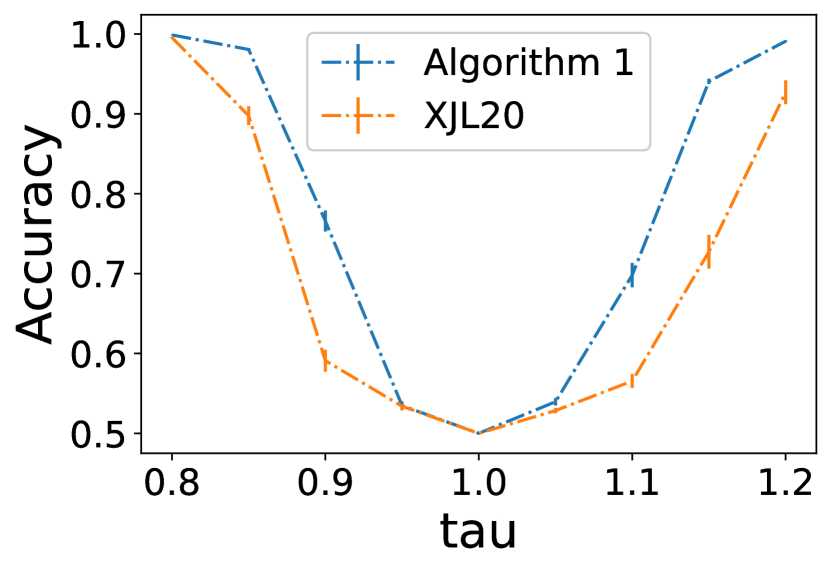
(a) $f=\operatorname{Nor}(0,1)$, $g=\operatorname{Nor}(0,\tau)$.

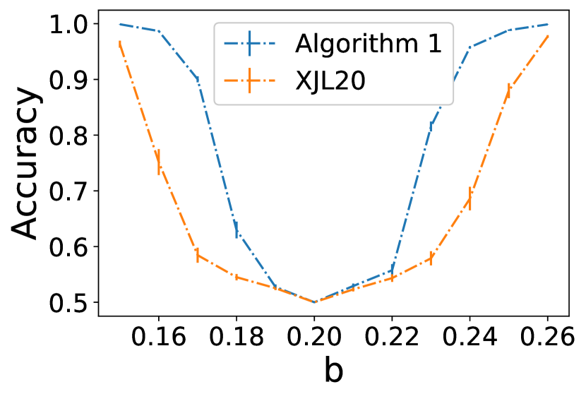
(b) $f=\operatorname{Geo}(0.2)$, $g=\operatorname{Geo}(b)$.

Figure 2: Accuracy of Algorithm 1 and the algorithm in [55] on data sampled from numerical SBMs of $N=400$ nodes and $K=2$ blocks; with (a) normal and (b) geometric interaction distributions. Results are averaged over $25$ samples. Error bars display empirical standard deviations.

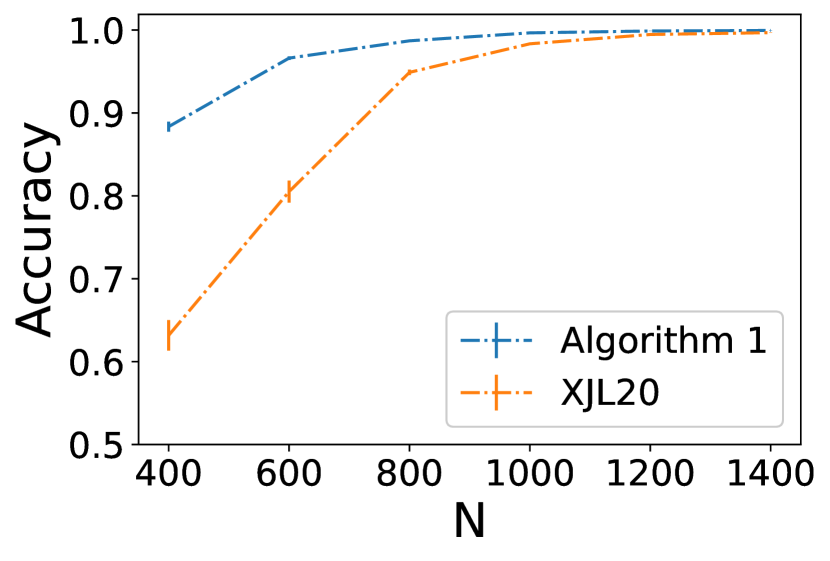
(a) $\tilde{f}=\operatorname{Nor}(0,1)$,
        $\tilde{g}=\operatorname{Nor}(0,1.2)$.

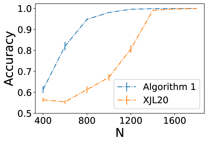
(b) $\tilde{f}=\operatorname{Nor}(0,1.3^{2}+1)$,
$\tilde{g}=\frac{1}{2}\operatorname{Nor}(-1.3,1)+\frac{1}{2}\operatorname{Nor}(1.3,1)$.

Figure 3: Accuracy of Algorithm 1 and the algorithm in [55] as a function of the number of nodes $N$ for $K=2$ blocks. Data are sampled from zero-inflated interaction distributions $f=\frac{1}{2}\delta_{0}+\frac{1}{2}\tilde{f}$ and $g=\frac{1}{2}\delta_{0}+\frac{1}{2}\tilde{g}$ with (a) normal, (b) mixed normal distributions $\tilde{f},\tilde{g}$. Results are averaged over $25$ samples.

5.2 Temporal networks

We study community recovery from temporal network data sampled from a stationary Markov SBM described in Section 4. We focus on sparse settings where the average degree per snapshot is of constant order, so that consistent recovery using a single snapshot is impossible, but consistent and even strongly consistent community recovery is possible when the number of snapshots $T$ is large enough (Remark 4.6).

5.2.1 Offline recovery

In an offline setting we apply the generic Algorithm 1 with vector-valued interactions initialised using $\mathcal{A}=\{x\in\{0,1\}^{T}\colon\log\frac{f}{g}(x)\leq\log\frac{f}{g}(0)\}$. Figure 4 presents the algorithm’s accuracy on a stationary Markov SBM where the intra- and inter-block interactions are indistinguishable for any single snapshot ($\mu_{1}=\nu_{1}$), and communities can be identified only by the different link persistence rates $P_{11}$ and $Q_{11}$ within and between communities. As expected, the accuracy of community recovery is low for $P_{11}\approx Q_{11}$. Outside such parameter regions, the performance of Algorithm 1 is remarkably high, even though each single snapshot alone carries no information about the community structure.

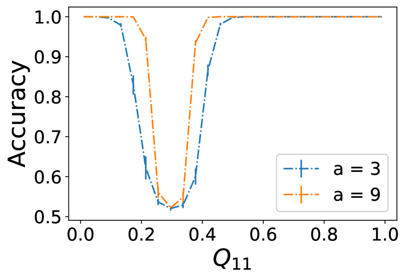
(a) $P_{11}=0.3$.

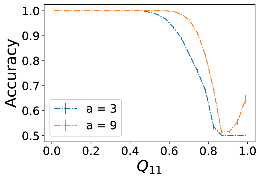
(b) $P_{11}=0.9$.

Figure 4: Performance of Algorithm 1 on a temporal network of $N=400$ nodes, $K=2$ blocks, and $T=60$ snapshots, as a function of inter-block link persistence $Q_{11}$. Data are sampled from a stationary Markov SBM with equal intra- and inter-block link densities $\mu_{1}=\nu_{1}=\frac{a}{N}$, and intra-block link persistence (a) $P_{11}=0.3$, (b) $P_{11}=0.9$. Results are averaged over 10 samples.

5.2.2 Online recovery with known interaction parameters

Figure 5 illustrates the number of snapshots needed to recover communities accurately using Algorithm 2, initiated either by spectral clustering or a blind random guess. In a sufficiently dense case (Figure 5(a)), spectral clustering on the first snapshot works well, and even a blind random guess leads to accurate results after a handful of iterations. In a sparser case (Figure 5(b)), spectral clustering on the first snapshot performs poorly, but a few online updates rapidly improve accuracy. Remarkably in both cases, a modest number of online updates yields a high accuracy, regardless of the quality of the initial clustering.

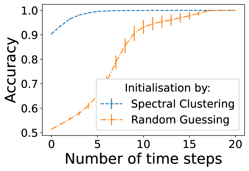
(a) $\mu_{1}=\frac{15}{N}$

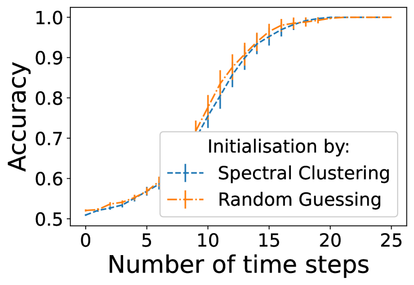
(b) $\mu_{1}=\frac{5}{N}$

Figure 5: Performance of Algorithm 2 as a function of the number of snapshots $T$ in a temporal network of $N=500$ nodes and $K=2$ blocks. Data are sampled from a stationary Markov SBM with intra-block link density (a) $\mu_{1}=\frac{15}{N}$, (b) $\mu_{1}=\frac{5}{N}$; inter-block link density $\nu_{1}=\frac{5}{N}$; and intra- and inter-block link persistence parameters $P_{11}=0.7$ and $Q_{11}=0.4$. Results are averaged over 25 samples.

5.2.3 Online recovery with unknown interaction parameters

When the interaction parameters are unknown, we replace Algorithm 2 with Algorithm 3, which adaptively estimates the interaction parameters jointly with community recovery. Figure 6 compares these algorithms in a sparse setting in which spectral clustering on a single snapshot does not provide much more information than a blind random guess. We see that a modest number of additional snapshots suffices to compensate for the need to estimate interaction parameters from data on the fly.

(a) $\mu_{1}=\nu_{1}=\frac{2}{N}$.

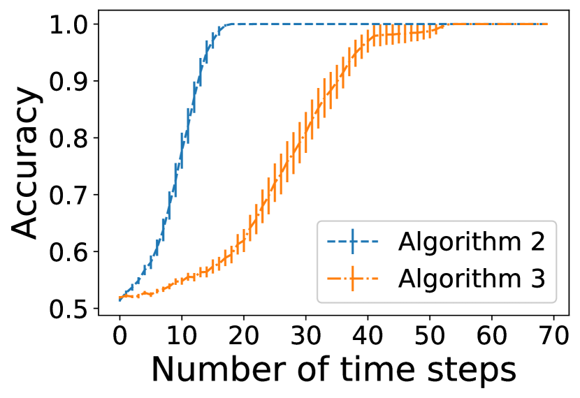
(b) $\mu_{1}=\frac{8}{N}$,  $\nu_{1}=\frac{2}{N}$.

Figure 6: Performance of Algorithms 2 and 3 as a function of the number of snapshots $T$ in a temporal network of $N=400$ nodes and $K=2$ blocks. Data are sampled from a stationary Markov SBM with intra- and inter-block link densities (a) $\mu_{1}=\nu_{1}$, (b) $\mu_{1}=4\nu_{1}$; and intra- and inter-block link persistence parameters $P_{11}=0.6$ and $Q_{11}=0.3$. Results are averaged over $25$ samples.

5.3 Experiments on real data

We investigate three data sets collected during three consecutive years from a high school Lycée Thiers in Marseilles, France [13, 35]. Nodes correspond to students, interactions to close-proximity encounters, and communities to classes, with about 40 students per class. We restrict to a subset of data corresponding to $K=3$ classes labelled PC, PC^∗ and PSI^∗, as they are present in each of the data sets. The performance of Algorithm 3 is compared against three reference algorithms:

• mean-adjacency [46], based on eigenvectors of the time-averaged adjacency matrix $\bar{X}=\frac{1}{T}\sum_{t=1}^{T}X^{t}$;

• mean normalised Laplacian [4], based on eigenvectors of the normalised Laplacian of $\bar{X}=\frac{1}{T}\sum_{t=1}^{T}X^{t}$;

• sum-of-squared [27], based on eigenvectors of the matrix $\sum_{t=1}^{T}((X^{t})^{2}-D^{t})$, where $D^{t}$ is the diagonal matrix with entries $D^{t}_{ii}=\sum_{j=1}^{N}X_{ij}^{t}$.

Figure 7 summarises the results. The mean normalised Laplacian algorithm is highly accurate in several cases, but is prone to large fluctuations. In contrast, Algorithm 3 displays a stable performance over time. The mean-adjacency and sum-of-squared algorithms perform poorly for each of the three data sets. We emphasise that the networks are very sparse, with the average degrees per snapshot in the three data sets being $0.04$, $0.02$, and $0.06$. This explains why a large number of snapshots is needed for community recovery.

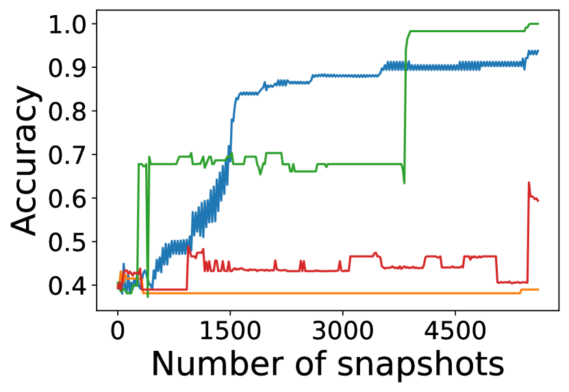
(a) Year $2011$.

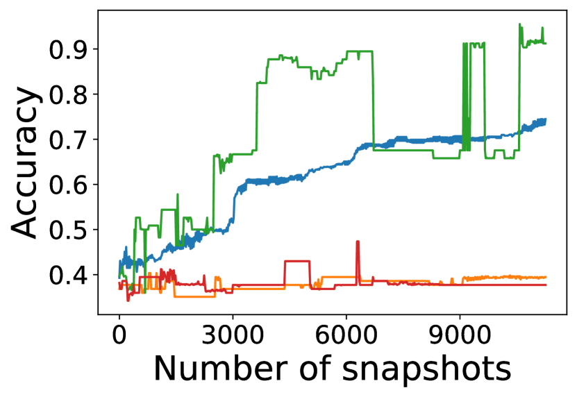
(b) Year 2012.

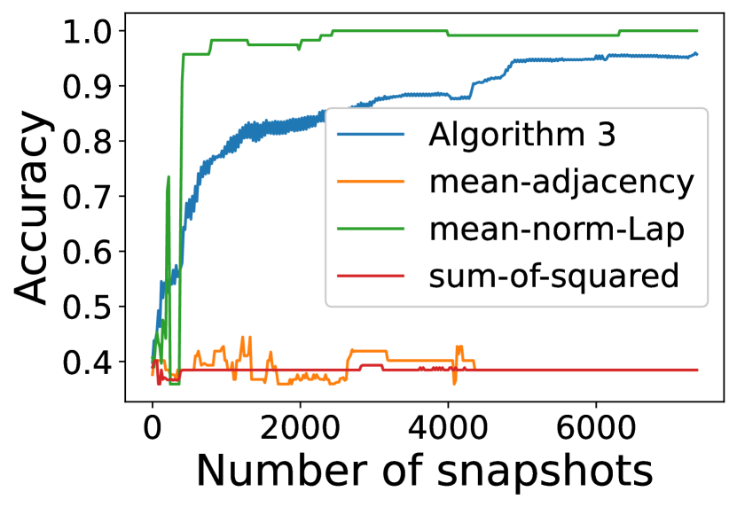
(c) Year 2013.

Figure 7: Performance of Algorithm 3 vs. three reference algorithms on high school data sets.

6 Technical comparison with related work

Let us discuss our contributions with respect to the most closely related earlier works.

Jog and Loh [25] discovered that the Rényi divergence provides a sharp quantity for strong consistency in homogeneous SBMs with discrete interaction distributions which are sparse in the sense of (3.2); recall Example 3.8. They analysed the MLE for networks of density $\rho\asymp\frac{\log N}{N}$, assuming that the conditional probability densities $\tilde{f},\tilde{g}$ in (3.2) do not depend on scale, are strictly positive either with respect to the counting measure on the positive integers or the Lebesgue measure on the real line, and are bounded by $||\log\frac{\tilde{f}}{\tilde{g}}||_{\infty}=O(1)$. The latter condition is not satisfied for several cases of interest, for example normal distributions with equal variances but unequal means. Part (ii) of Theorem 3.7 generalises the setting of [25] to arbitrary probability measures on an arbitrary measurable space, and does not require the condition $||\log\frac{\tilde{f}}{\tilde{g}}||_{\infty}=O(1)$.

Yun and Proutière [57] consider interactions on a finite space and obtain consistency results similar to Theorem 3.2 but with additional regularity conditions, which in the homogeneous case correspond to $||\log\frac{f}{g}||_{\infty}=O(1)$ and $\sum_{x\neq 0}(f(x)-g(x))^{2}=\Omega(\rho^{2})$ with $\rho=\max_{x\neq 0}\left(f(x),g(x)\right)\gg N^{-1}$. For the consistency of a spectral clustering algorithm, they also impose $N\min_{x\neq 0}(f(x)\wedge g(x))\ \geq\ (N\rho)^{\Omega(1)}$. In contrast to [25, 55], the analysis in [57] is valid also for inhomogeneous SBMs with unbalanced block sizes. We believe that Theorems 3.1 and 3.2 could be extended to similar generality, at the cost of longer and more technical proofs to account for the lack of symmetry.

Xu, Jog, and Loh [55] is a major contribution to the study of homogeneous SBMs with unknown interactions, but still relies on several restrictive assumptions. First, their consistency analysis is restricted to interaction distributions having an atom at zero, thereby ruling out purely continuous distributions (e.g. Example 3.5). Also, the analysis does not extend to discrete probability distributions with infinite support (e.g. Examples 3.4, 3.13, and 3.14); nor interactions distributions with finite support of size growing with $N$ (e.g. temporal networks with $T\gg 1$). Moreover, some additional technical conditions are needed, such as the existence of two blocks of sizes $N_{\rm min}$ and $N_{\rm min}+1$ where $N_{\rm min}$ is the minimum block size (see [55, Theorem 2]), as well as some technical smoothness conditions which may be difficult to verify in practice. Theorems 3.1 and Theorem 3.2 generalise the framework of [55] to a setting which requires neither regularity assumptions on $f,g$ nor restrictions on the underlying space $\mathcal{S}$ of interaction types. Theorem 3.11 is similar in spirit to upper bounds in [55] and [57] which perform initial clustering using $\mathcal{A}=\{0\}$, but is fundamentally different in that it makes no assumptions about truncating the label space $\mathcal{S}$, nor any assumptions about the regularity of the interaction distributions $f,g$. Moreover, for temporal binary interactions with $\mathcal{S}=\{0,1\}^{T}$, the algorithms in [55] are of exponential complexity in $T$.

Paul and Chen [45] is a key contribution on the recovery thresholds for multilayer SBMs, assuming uncorrelated layers. Section 4 contains both information-theoretic and algorithmic contributions to clustering temporally correlated networks. Theorems 4.2 and 4.5 extend the setting of [45] to correlated layers. In addition, the optimal misclassification rate in Theorem 3.2 extends [45, Theorem 6] to non-binary settings (recall Example 3.6). We developed Algorithms 2 and 3 for online community recovery in temporal networks. These algorithms are designed to accurately utilise information related to temporal correlation patterns, and as such are radically different from the mainstream of methods [7, 8, 27, 45, 46] relying on spectral clustering of layer-aggregated adjacency matrices.

7 Conclusions and future work

In this paper, we studied community recovery in non-binary and dynamic stochastic block models. Unlike most earlier works, our analysis allows the shape and size of the interaction space to be scale-dependent, which enables us to study correlated interaction patterns over short and long time horizons. For clarity, most consistency results were stated under the assumption that the number of blocks is bounded, but quantitative bounds in Theorem 3.1 allow several generalisations to cases with $K\gg 1$. We proposed Algorithm 1 that fully utilises the non-binary nature of the observed data for recovering community memberships. Unlike earlier methods, Algorithm 1 is provably consistent for general interaction distributions (not requiring atoms), including standard continuous distributions such as normal and exponential. Our analysis of consistency essentially requires bounded Rényi divergences of order 3/2. Investigating whether this condition can be relaxed remains an open problem.

For temporal and multiplex networks, we proposed Algorithms 2 and 3 for community recovery based on fast online likelihood updating, and investigated their performance with numerical experiments on synthetic and real data. We observed that even in sparse or low-information regimes, both algorithms appear to produce accurate results given a reasonable number of temporal snapshots. The theoretical consistency analysis of these algorithms remains an open problem.

This work has been done within the project of Inria - Nokia Bell Labs “Distributed Learning and Control for Network Analysis” and was partially supported by COSTNET Cost Action CA15109.

Appendix A Preliminaries

A.1 Table of notations

We keep the same notations as in the main text. Additionally, we define $Z_{\alpha}(f\|g)=\int f^{\alpha}g^{1-\alpha}$, so that $D_{\alpha}(f\|g)=(\alpha-1)^{-1}\log Z_{\alpha}(f\|g)$. We also denote by $d_{\rm KL}(f\|g)=\int f\log\frac{f}{g}$ the Kullback-Leibler divergence between $f$ and $g$ and we introduce $v_{\rm KL}(f\|g)=\int f\log^{2}\frac{f}{g}-d_{\rm KL}^{2}(f\|g)$. Table 1 summarises commonly used notations in the article.

Symbol	Meaning
$\delta_{x}$	Dirac measure at $x$
$\delta_{ab}$	Kronecker delta
$\rho$	Overall density parameter
$\eta$	Scale parameter
$N$	Number of nodes
$K$	Number of communities (blocks)
$T$	Number of snapshots (temporal networks)
$\mathcal{S}$	Space of interaction types $(\mathcal{S}=\{0,1\}^{T}$ for temporal networks)
$\mathcal{X}$	Space of observations
$\mathcal{Z}$	Space of node labellings (subset of $[K]^{[N]}$)
$i,j$	Node indices
$k,\ell$	Community (block) indices
$\sigma$	Node labelling ($\sigma\in[K]^{N}$)
$X=\left(X_{ij}\right)$	Data array ($X\in\mathcal{S}^{N\times N}$)
$f(x)$, $g(x)$	Probability of an interaction of type $x\in\mathcal{S}$ between two nodes
$\mu_{a}$, $\nu_{a}$	Initial intra- and inter-block interaction distributions, $a\in\{0,1\}$ (for Markov dynamics)
$P_{ab}$, $Q_{ab}$	Probability of transition $a\to b$ ($a,b\in\{0,1\})$ for intra- and inter-block interactions
$D_{\alpha}(f\|g)$	Rényi divergence of order $\alpha$
$D^{s}_{\alpha}(f,g)$	Symmetric Rényi divergence of order $\alpha$
$Z_{\alpha}(f\|g)$	Hellinger integrals
$\mathrm{Hel}(f,g)$	Hellinger distance
$\beta_{r}(f,g)$	Rényi divergence ratio (defined in (E.2))
$\operatorname{Ham}(\sigma_{1},\sigma_{2})$	Hamming distance
$\operatorname{Ham}^{*}(\sigma_{1},\sigma_{2})$	Absolute classification error
$\operatorname{Mir}(\sigma_{1},\sigma_{2})$	Mirkin distance

Table 1: Common notations.

A.2 Multinomial concentration

Fix integers $N,K\geq 1$, and consider the space $[K]^{N}$ of mappings $\sigma:[N]\to[K]$. For any such mapping, we denote the frequencies of output values by $N_{k}(\sigma)=\sum_{i=1}^{N}\delta_{\sigma(i)k}$ for $k=1,\dots,K$. When the space $[K]^{N}$ is equipped with a probability measure $\mathbb{P}$, then $\sigma\mapsto(N_{1}(\sigma),\dots,N_{K}(\sigma))$ is considered as a random variable. Given $\epsilon>0$ and $\alpha_{1},\dots,\alpha_{K}\in[0,1]$, we shall be interested in probabilities of events of the form

$$\mathcal{A}_{\epsilon} \ =\ \Big{\{}\sigma:{\lvert N_{k}(\sigma)-\alpha_{k}N\rvert}\leq\epsilon\alpha_{k}N\ \text{for all $k\in[K]$}\Big{\}},$$ (A.1)

$$\mathcal{A}_{\epsilon,+} \ =\ \Big{\{}\sigma:N_{k}(\sigma)\geq(1-\epsilon)\alpha_{k}N\ \text{for all $k\in[K]$}\Big{\}}.$$ (A.2)

Lemma A.1.

Let $0<\epsilon\leq 1$.

1. If $\mathbb{P}=\alpha^{\otimes N}$ for a probability measure $\alpha$ on $[K]$, then $\mathbb{P}(\mathcal{A}_{\epsilon}^{c})\leq 2\sum_{k=1}^{K}e^{-(\epsilon^{2}/3)\alpha_{k}N}$ and $\mathbb{P}(\mathcal{A}_{\epsilon,+}^{c})\leq\sum_{k=1}^{K}e^{-(\epsilon^{2}/2)\alpha_{k}N}$.

2. If $\mathbb{P}$ is the uniform distribution on $[K]^{N}$, then $\mathbb{P}(\mathcal{A}_{\epsilon}^{c})\leq 2e^{\log K-\epsilon^{2}N/(3K)}$ and $\mathbb{P}(\mathcal{A}_{\epsilon,+}^{c})\leq e^{\log K-\epsilon^{2}N/(2K)}$.

Proof.

(i) Because $N_{k}$ is $\operatorname{Bin}(N,\alpha_{k})$-distributed, a Chernoff bound [24, Corollary 2.3] implies that

$$\mathbb{P}({\lvert N_{k}(\sigma)-\alpha_{k}N\rvert}>\epsilon\alpha_{k}N)\ \leq\ 2e^{-(\epsilon^{2}/3)\alpha_{k}N}.$$

Similarly, another Chernoff bound [24, Theorem 2.1] implies that

$$\mathbb{P}(N_{k}(\sigma)\leq(1-\epsilon)\alpha_{k}N)\ \leq\ e^{-(\epsilon^{2}/2)\alpha_{k}N}.$$

Hence the first claim follows by the union bound.

(ii) The second claim follows immediately from (i) after noting that the uniform distribution on $[K]^{N}$ can be represented as $\pi=\alpha^{\otimes N}$ where $\alpha_{k}=K^{-1}$ for all $k$. ∎

We shall also be interested in random variables defined by $N_{\rm min}(\sigma)=\min_{k}N_{k}(\sigma)$ and $\Delta N(\sigma)=\max_{k,\ell}{\lvert N_{k}(\sigma)-N_{\ell}(\sigma)\rvert}$. The following result implies that for large-scale uniformly distributed settings with $N\gg K\log K$, these random variables are bounded by $N_{\rm min}\geq(1-\epsilon)K^{-1}N$ and $\Delta N\leq 2\epsilon K^{-1}N$ with high probability for $(\frac{K\log K}{N})^{1/2}\ll\epsilon\leq 1$. For example, we may select $\epsilon=(\frac{K\log K}{N})^{0.499}$.

Lemma A.2.

Let $0<\epsilon\leq 1$. (i) If $\mathbb{P}=\alpha^{\otimes N}$ for a probability measure $\alpha$ on $[K]$, then

$$\mathbb{P}\Big{(}N_{\rm min}\geq(1-\epsilon)\alpha_{\rm min}N\Big{)} \ \geq\ 1-\delta_{1},$$ (A.3)

$$\mathbb{P}\Big{(}\Delta N\leq(2\epsilon\alpha_{\rm max}+\Delta\alpha)N\Big{)} \ \geq\ 1-\delta_{2},$$

where $\delta_{1}=Ke^{-(\epsilon^{2}/2)\alpha_{\rm min}N}$ and $\delta_{2}=2Ke^{-(\epsilon^{2}/3)\alpha_{\rm min}N}$, together with $\alpha_{\rm min}=\min_{k}\alpha_{k}$, $\alpha_{\rm max}=\max_{k}\alpha_{k}$, and $\Delta\alpha=\max_{k,\ell}{\lvert\alpha_{k}-\alpha_{\ell}\rvert}$.

(ii) If $\mathbb{P}$ is the uniform distribution on $[K]^{N}$, then

$$\mathbb{P}\Big{(}N_{\rm min}\geq(1-\epsilon)K^{-1}N\Big{)} \ \geq\ 1-\delta_{1},$$

$$\mathbb{P}\Big{(}\Delta N\leq 2\epsilon K^{-1}N\Big{)} \ \geq\ 1-\delta_{2},$$

with $\delta_{1}=e^{\log K-\epsilon^{2}N/(2K)}$ and $\delta_{2}=2e^{\log K-\epsilon^{2}N/(3K)}$.

Proof.

(i) By Lemma A.1, then events $\mathcal{A}_{\epsilon}$ and $\mathcal{A}_{\epsilon,+}$ defined by (A.1)–(A.2) satisfy $\mathbb{P}(\mathcal{A}_{\epsilon_{+}}^{c})\leq\delta_{1}$ and $\mathbb{P}(\mathcal{A}_{\epsilon}^{c})\leq\delta_{2}$. On the event $\mathcal{A}_{\epsilon,+}$, $N_{\rm min}\geq(1-\epsilon)\alpha_{\rm min}N$. Hence the first inequality in (A.3) follows. For the second inequality, we note that on the event $\mathcal{A}_{\epsilon}$

$${\lvert N_{k}-N_{\ell}\rvert} \ \leq\ {\lvert N_{k}-\alpha_{k}N\rvert}+{\lvert N_{\ell}-\alpha_{\ell}N\rvert}+{\lvert\alpha_{k}N-\alpha_{\ell}N\rvert}$$

$$\ \leq\ \epsilon\alpha_{k}N+\epsilon\alpha_{\ell}N+{\lvert\alpha_{k}-\alpha_{\ell}\rvert}N$$

$$\ \leq\ 2\epsilon\alpha_{\rm max}N+\Delta\alpha N$$

for all $k,\ell$. This confirms the second inequality in (A.3).

(ii) This follows immediately from (i) after noting that the uniform distribution on $[K]^{N}$ can be represented as $\pi=\alpha^{\otimes N}$ where $\alpha_{k}=K^{-1}$ for all $k$. ∎

A.3 Elementary analysis

Lemma A.3.

For any integer $j\geq 1$ and any real number $0\leq q<1$,

$$\sum\limits_{k=j}^{\infty}\binom{k}{j}q^{k-j}=(1-q)^{-(j+1)}.$$

Proof.

Denote the falling factorial by $(x)_{j}=x(x-1)\cdots(x-j+1)$, and let $f(q)=(1-q)^{-1}$. Then the $j$-th derivative of $f$ equals $f^{(j)}(q)=j!(1-q)^{-(j+1)}$. Because $f(q)=\sum_{k=0}^{\infty}q^{k}$, we find that the $j$-th derivative of $f$ also equals $\sum_{k=j}^{\infty}(k)_{j}q^{k-j}$. Hence the claim follows. ∎

Lemma A.4.

(i) For $t\geq 0$, $\log(1+t)=t-\epsilon_{1}$ where $0\leq\epsilon_{1}\leq\frac{1}{2}t^{2}$. (ii) For $0\leq t<1$, $\log(1-t)=-t-\epsilon_{2}$ where $0\leq\epsilon_{2}\leq\frac{t^{2}}{2(1-t)^{2}}$, and especially, $0\leq\epsilon_{2}\leq 2t^{2}$ for $0\leq t\leq\frac{1}{2}$.

Proof.

(i) By taking two derivatives of $t\mapsto\log(1+t)$, we find that $\log(1+t)=t-\epsilon_{1}$ with $\epsilon_{1}=\int_{0}^{t}\int_{0}^{s}(1+u)^{-2}duds$.

(ii) Similarly, we find that $\log(1-t)=-t-\epsilon_{2}$ with $\epsilon_{2}=\int_{0}^{t}\int_{0}^{s}(1-u)^{-2}duds$. ∎

Lemma A.5.

For any $0\leq x\leq\frac{1}{2}$ and $a>0$, the error term in the approximation $(1-x)^{a}=1-ax-r(x)$ is bounded by ${\lvert r(x)\rvert}\leq\frac{2{\lvert a-1\rvert}}{2^{a}}ax^{2}$. Moreover, $r(x)\geq 0$ when $a\geq 1$.

Proof.

The error term in the approximation $f(x)=f(0)+f^{\prime}(0)x+r(x)$ equals $r(x)=\int_{0}^{x}\int_{0}^{t}f^{\prime\prime}(s)dsdt$ and is bounded by ${\lvert r(x)\rvert}\leq\frac{1}{2}cx^{2}$ with $c=\max_{0\leq x\leq 1/2}{\lvert f^{\prime\prime}(x)\rvert}$. The function $f(x)=(1-x)^{a}$ satisfies $f(0)=1$ and $f^{\prime}(0)=-a$, together with $f^{\prime\prime}(x)=a(a-1)(1-x)^{a-2}$. The claims follow after noticing that

$$\max_{0\leq x\leq 1/2}{\lvert f^{\prime\prime}(x)\rvert}\ =\ \begin{cases}{\lvert f^{\prime\prime}(\tfrac{1}{2})\rvert}=\frac{4}{2^{a}}a{\lvert a-1\rvert}&\quad\text{for $0<a<2$},\\ f^{\prime\prime}(0)=a(a-1)&\quad\text{for $a\geq 2$}.\end{cases}$$

∎

Lemma A.6.

Fix $0\leq\delta<1$. Then the error term in the approximation $\sqrt{1-x}=1-\frac{1}{2}x-\epsilon(x)$ satisfies $0\leq\epsilon(x)\leq cx^{2}$ for all $0\leq x\leq\delta$, where $c=\frac{1}{8}(1-\delta)^{-3/2}$.

Proof.

Consider Taylor’s approximation $f(x)=f(0)+f^{\prime}(0)x+r(x)$ where $r(x)=\int_{0}^{x}\int_{0}^{t}f^{\prime\prime}(s)dsdt$ is bounded by $\frac{1}{2}c_{1}x^{2}\leq r(x)\leq\frac{1}{2}c_{2}x^{2}$ with $c_{1}=\min_{0\leq x\leq\delta}f^{\prime\prime}(x)$ and $c_{2}=\max_{0\leq x\leq\delta}f^{\prime\prime}(x)$. The function $f(x)=(1-x)^{1/2}$ satisfies $f(0)=1$ and $f^{\prime}(0)=-\frac{1}{2}$, together with $f^{\prime\prime}(x)=-\frac{1}{4}(1-x)^{-3/2}$. Now $c_{1}=-\frac{1}{4}(1-x)^{-3/2}$ and $c_{2}=-\frac{1}{4}\leq 0$. Hence the claim is true with $\epsilon(x)=-r(x)$. ∎

Lemma A.7.

For any $0\leq p_{1},\dots,p_{n}\leq 1$, $A-B\leq 1-\prod_{i}(1-p_{i})\leq A$ with $A=\sum_{i}p_{i}$ and $B=\frac{1}{2}\sum_{i}\sum_{j\neq i}p_{i}p_{j}$.

Proof.

Let $E_{1},\dots,E_{n}$ be independent events with probabilities $p_{1},\dots,p_{n}$. Apply inclusion–exclusion to the probability of the event $E=\cup_{i}E_{i}$ having probability $\mathbb{P}(\cup_{i}E_{i})=1-\mathbb{P}(\cap_{i}E_{i}^{c})=1-\prod_{i}(1-p_{i})$. ∎

Lemma A.8.

For any integer $M\geq 1$ and any number $0\leq s<1$,

$$Ms^{M}\ \leq\ \sum_{m=M}^{\infty}ms^{m}\ \leq\ (1-s)^{-2}Ms^{M}.$$

Proof.

Denote $S=\sum_{m=M}^{\infty}ms^{m}$. By differentiating $\sum_{m=M}^{\infty}s^{m}=(1-s)^{-1}s^{M}$, we find that

$$s^{-1}S\ =\ \sum_{m=M}^{\infty}ms^{m-1}\ =\ (1-s)^{-2}s^{M}+(1-s)^{-1}Ms^{M-1},$$

from which we see that

$$S\ =\ s(1-s)^{-2}\Big{(}s^{M}+(1-s)Ms^{M-1}\Big{)}\ =\ \frac{Ms^{M}}{(1-s)^{2}}\Big{(}1-s(1-1/M)\Big{)}$$

The upper bound now follows from $1-s(1-1/M)\leq 1$. The lower bound is immediate, corresponding to the first term of the nonnegative series. ∎

A.4 Hamming distances

Lemma A.9.

For any node labelling $\sigma:[N]\to[K]$, the number $Z_{\sigma,m}$ of node labellings $\sigma^{\prime}:[N] \to[K]$ such that $\operatorname{Ham}(\sigma,\sigma^{\prime})=m$ satisfies

$$Z_{\sigma,m}\ =\ \binom{N}{m}(K-1)^{m}\ \leq\ \left(\frac{eN(K-1)}{m}\right)^{m}.$$

Proof.

Any node labelling $\sigma^{\prime}:[N]\to[K]$ which differs from a particular $\sigma$ at exactly $m$ input values can be constructed as follows. First choose a set of $m$ input values out of $N$; there are $\binom{N}{m}$ ways to do this. Then for each $i$ of the chosen $m$ input values, select a new output value from the of $K-1$ values excluding $\sigma(i)$; there are $(K-1)^{m}$ ways to do this. Hence the equality follows.

To verify the inequality, we note that $\frac{m^{m}}{m!}\leq\sum_{s=0}^{\infty}\frac{m^{s}}{s!}=e^{m}$. Therefore, we see that $\binom{N}{m}\leq\frac{N^{m}}{m!}\leq(\frac{eN}{m})^{m}$, and the inequality follows. ∎

Appendix B Comparing partitions

B.1 Classification error

The absolute classification error between node labellings $\sigma,\sigma^{\prime}:[N]\to[K]$ is defined by

$$\operatorname{Ham}^{*}(\sigma,\sigma^{\prime})\ =\ \min_{\rho\in\operatorname{Sym}(K)}\operatorname{Ham}(\sigma,\rho\circ\sigma^{\prime}),$$

where $\operatorname{Ham}(\sigma,\sigma^{\prime})=\sum_{i=1}^{N}1(\sigma(i)\neq\sigma^{\prime}(i))$ denotes the Hamming distance and $\operatorname{Sym}(K)$ denotes the group of permutations on $[K]$. We note that $\operatorname{Ham}^{*}(\sigma,\sigma^{\prime})=\operatorname{Ham}^{*}(\rho\circ\sigma,\rho^{\prime}\circ\sigma^{\prime})$ for all $\rho,\rho^{\prime}\in\operatorname{Sym}(K)$, which confirms that the classification error depends on its inputs only via the partitions induced by the preimages of the node labellings. The relative error $N^{-1}\operatorname{Ham}^{*}(\sigma,\sigma^{\prime})$ is usually called the classification error [39, 38].

B.2 Mirkin distance

The Mirkin distance is one of the common pair-counting based cluster validity indices [17, 29]. It is defined between two nodes labellings $\sigma,\sigma^{\prime}:[N]\to[K]$ by

$$\operatorname{Mir}(\sigma,\sigma^{\prime})\ =\ 2\sum_{1\leq i<j\leq N}\big{(}e_{ij}(1-e^{\prime}_{ij})+(1-e_{ij})e^{\prime}_{ij}\big{)}$$

where $e_{ij}=1(\sigma(i)=\sigma(j))$ and $e^{\prime}_{ij}=1(\sigma^{\prime}(i)=\sigma^{\prime}(j))$. The Mirkin distance is related to the Rand index by $\operatorname{Mir}(\sigma,\sigma^{\prime})=N(N-1)(1-\operatorname{Rand}(\sigma,\sigma^{\prime}))$.

For any node labelling $\sigma:[N]\to[K]$, we denote by $E(\sigma)$ the set of unordered node pairs $\{i,j\}$ such that $\sigma(i)=\sigma(j)$, by $N_{\rm min}^{\sigma}=\min_{k}{\lvert C_{k}\rvert}$ and $N_{\rm max}^{\sigma}=\max_{k}{\lvert C_{k}\rvert}$ where $C_{k}=\{i:\sigma(i)=k\}$. Then we note that the Mirkin distance can be written as

$$\operatorname{Mir}(\sigma,\sigma^{\prime})\ =\ 2\left({\lvert E(\sigma)\setminus E(\sigma^{\prime})\rvert}+{\lvert E(\sigma^{\prime})\setminus E(\sigma)\rvert}\right).$$ (B.1)

The following result shows that when the Mirkin metric is small, then the maximum set sizes in two partitions cannot differ arbitrarily much.

Lemma B.1.

For any node labellings $\sigma,\sigma^{\prime}:[N]\to[K]$,

$${\lvert E(\sigma)\setminus E(\sigma^{\prime})\rvert}\ \geq\ \frac{1}{2}(N_{\rm max}^{\sigma}-N_{\rm max}^{\sigma^{\prime}})N_{\rm max}^{\sigma}.$$

Proof.

For any $k$, denote by $E(C_{k})$ the set of unordered node pairs in $C_{k}$. Also denote $N_{k}=|E(C_{k})|$, $N^{\prime}_{\ell}=|E(C^{\prime}_{\ell})|$, and $N_{k\ell}={\lvert C_{k}\cap C^{\prime}_{\ell}\rvert}$. Then we find that

$${\lvert E(C_{k})\setminus E(\sigma^{\prime})\rvert}\ =\ \binom{N_{k}}{2}-\sum_{\ell}\binom{N_{k\ell}}{2}.$$

By applying the bound $N_{k\ell}\leq N_{\rm max}^{\sigma^{\prime}}$, we see that

$$\sum_{\ell}\binom{N_{k\ell}}{2}\ \leq\ \frac{1}{2}(N_{\rm max}^{\sigma^{\prime}}-1)\sum_{\ell}N_{k\ell}\ =\ \frac{1}{2}(N_{\rm max}^{\sigma^{\prime}}-1)N_{k}.$$

Therefore,

$${\lvert E(C_{k})\setminus E(\sigma^{\prime})\rvert}\ \geq\ \binom{N_{k}}{2}-\frac{1}{2}(N_{\rm max}^{\sigma^{\prime}}-1)N_{k}\ \geq\ \frac{1}{2}(N_{k}-N_{\rm max}^{\sigma^{\prime}})N_{k}.$$

The claim now follows after noting that

$${\lvert E(\sigma)\setminus E(\sigma^{\prime})\rvert}\ =\ \sum_{k}{\lvert E(C_{k})\setminus E(\sigma^{\prime})\rvert}\ \geq\ \max_{k}{\lvert E(C_{k})\setminus E(\sigma^{\prime})\rvert}.$$

∎

B.3 Optimal alignments

The confusion matrix of node labellings $\sigma,\sigma^{\prime}:[N]\to[K]$ is the $K$-by-$K$ matrix having entries

$$N_{k\ell}\ =\ {\lvert C_{k}\cap C^{\prime}_{\ell}\rvert},$$

where $C_{k}=\sigma^{-1}(k)$ and $C^{\prime}_{\ell}=(\sigma^{\prime})^{-1}(\ell)$. We say that node labellings $\sigma,\sigma^{\prime}:[N]\to[K]$ are optimally aligned if

$$\operatorname{Ham}^{*}(\sigma,\sigma^{\prime})\ =\ \operatorname{Ham}(\sigma,\sigma^{\prime}).$$ (B.2)

The following result provides an entrywise upper bound for the confusion matrix of optimally aligned node labellings.

Lemma B.2.

If $\sigma$ and $\sigma^{\prime}$ are optimally aligned, then the associated confusion matrix is bounded by

$$N_{k\ell}+N_{\ell k}\ \leq\ N_{kk}+N_{\ell\ell}$$ (B.3)

and

$$N_{k\ell}\ \leq\ \frac{1}{3}(N_{k}+N^{\prime}_{\ell})$$ (B.4)

for all $k\neq\ell$, where $N_{k}=\sum_{\ell}N_{k\ell}$ and $N^{\prime}_{\ell}=\sum_{k}N_{k\ell}$.

Proof.

Fix some distinct $k,\ell\in[K]$. Define $\sigma^{\prime\prime}=\tau\circ\sigma^{\prime}$ where $\tau$ is the $K$-permutation which swaps $k$ and $\ell$ and leaves other elements of $[K]$ intact. Denote $C^{\prime\prime}_{j}=(\sigma^{\prime\prime})^{-1}(j)$. Then we see that $C^{\prime\prime}_{j}=C^{\prime}_{\ell}$ for $j=k$, $C^{\prime\prime}_{j}=C^{\prime}_{k}$ for $j=\ell$, and $C^{\prime\prime}_{j}=C^{\prime}_{j}$ otherwise. Using the formulas

$$\operatorname{Ham}(\sigma,\sigma^{\prime})=\sum_{j}{\lvert C_{j}\setminus C^{\prime}_{j}\rvert}\qquad\text{and}\qquad\operatorname{Ham}(\sigma,\sigma^{\prime\prime})=\sum_{j}{\lvert C_{j}\setminus C^{\prime\prime}_{j}\rvert}$$

we find that

$$\operatorname{Ham}(\sigma,\sigma^{\prime\prime})-\operatorname{Ham}(\sigma,\sigma^{\prime})\ =\ {\lvert C_{k}\setminus C^{\prime}_{\ell}\rvert}-{\lvert C_{k}\setminus C^{\prime}_{k}\rvert}+{\lvert C_{\ell}\setminus C^{\prime}_{k}\rvert}-{\lvert C_{\ell}\setminus C^{\prime}_{\ell}\rvert}.$$

Because

$${\lvert C_{k}\setminus C^{\prime}_{\ell}\rvert}-{\lvert C_{k}\setminus C^{\prime}_{k}\rvert} \ =\ (N_{k}-N_{k\ell})-(N_{k}-N_{kk})\ =\ N_{kk}-N_{k\ell},$$

and the same formula holds also with the roles of $k$ and $\ell$ swapped, it follows that

$$\operatorname{Ham}(\sigma,\sigma^{\prime\prime})-\operatorname{Ham}(\sigma,\sigma^{\prime})\ =\ N_{kk}-N_{k\ell}+N_{\ell\ell}-N_{\ell k}.$$

Because $\sigma$ and $\sigma^{\prime}$ are optimally aligned, we see that $\operatorname{Ham}(\sigma,\sigma^{\prime})\leq\operatorname{Ham}(\sigma,\sigma^{\prime\prime})$. Therefore, the left side of the above equality is nonnegative, and (B.3) follows.

Next, by applying the bounds $N_{kk}\leq N_{k}-N_{k\ell}$ and $N_{\ell\ell}\leq N^{\prime}_{\ell}-N_{k\ell}$, we may conclude that

$$0\ \leq\ N_{kk}-N_{k\ell}+N_{\ell\ell}-N_{\ell k}\ \leq\ N_{k}+N^{\prime}_{\ell}-3N_{k\ell}-N_{\ell k}.$$

The inequality (B.4) now follows by noting that

$$N_{k\ell}\ \leq\ \frac{1}{3}(N_{k}+N^{\prime}_{\ell}-N_{\ell k})\ \leq\ \frac{1}{3}(N_{k}+N^{\prime}_{\ell}).$$

∎

B.4 Relating the classification error and the Mirkin distance

The next result provides a way to bound the absolute classification error $\operatorname{Ham}^{*}(\sigma,\sigma^{\prime})$ using the Mirkin distance $\operatorname{Mir}(\sigma,\sigma^{\prime})$.

Lemma B.3.

For any node labellings $\sigma,\sigma^{\prime}:[N]\to[K]$,

$${\lvert E(\sigma)\setminus E(\sigma^{\prime})\rvert}\ \geq\ \max\left\{N_{\rm min}^{\sigma}-\operatorname{Ham}^{*}(\sigma,\sigma^{\prime}),\ \frac{1}{3}N_{\rm min}^{\sigma}-\frac{1}{6}N_{\rm max}^{\sigma^{\prime}}\right\}\operatorname{Ham}^{*}(\sigma,\sigma^{\prime}).$$

Proof.

Let us note that all quantities appearing in the statement of the lemma remain invariant if we replace $\sigma^{\prime}$ by $\rho\circ\sigma^{\prime}$, where $\rho\in\operatorname{Sym}(K)$ is an arbitrary permutation. Therefore, we may without loss of generality assume that $\sigma$ and $\sigma^{\prime}$ are optimally aligned according to (B.2).

For sets $C,D\subset[N]$, we denote by $E(C,D)$ the collection of unordered pairs which can be written as $e=\{i,j\}$ with $i\in C$ and $j\in D$, and we denote the set of node pairs internal to $C$ by $E(C)=E(C,C)$. We observe that the set $\Gamma=E(\sigma)\setminus E(\sigma^{\prime})$ can be partitioned into $\Gamma=\cup_{k}\Gamma_{k}$, where $\Gamma_{k}=E(C_{k})\setminus E(\sigma^{\prime})$. We may further split this set according to $\Gamma_{k}=\Gamma_{k1}\cup\Gamma_{k2}$, where

$$\Gamma_{k1} \ =\ E(C_{k}\cap C^{\prime}_{k},\,C_{k}\setminus C^{\prime}_{k}),$$

$$\Gamma_{k2} \ =\ E(C_{k}\setminus C^{\prime}_{k})\setminus E(\sigma^{\prime}).$$

Therefore, it follows that ${\lvert\Gamma\rvert}=\sum_{k}({\lvert\Gamma_{k1}\rvert}+{\lvert\Gamma_{k2}\rvert}).$

To analyse the sizes of $\Gamma_{k1}$ and $\Gamma_{k2}$, denote $N_{k\ell}={\lvert C_{k}\cap C^{\prime}_{\ell}\rvert}$ and $D_{k}={\lvert C_{k}\setminus C^{\prime}_{k}\rvert}$. Then we immediately see that

$${\lvert\Gamma_{k1}\rvert}\ =\ N_{kk}D_{k}.$$ (B.5)

Furthermore, we see that $E(C_{k}\setminus C^{\prime}_{k})\cap E(\sigma^{\prime})=\cup_{\ell\neq k}E(C_{k}\cap C^{\prime}_{\ell}),$ and it follows that

$${\lvert\Gamma_{k2}\rvert}\ =\ {\lvert E(C_{k}\setminus C^{\prime}_{k})\rvert}-\sum_{\ell\neq k}{\lvert E(C_{k}\cap C^{\prime}_{\ell})\rvert}\ =\ \binom{D_{k}}{2}-\sum_{\ell\neq k}\binom{N_{k\ell}}{2}.$$ (B.6)

By combining (B.5)–(B.6) we conclude that

$${\lvert\Gamma\rvert}\ =\ \sum_{k}({\lvert\Gamma_{k1}\rvert}+{\lvert\Gamma_{k2}\rvert})\ =\ \sum_{k}\bigg{\{}N_{kk}D_{k}+\binom{D_{k}}{2}-\sum_{\ell\neq k}\binom{N_{k\ell}}{2}\bigg{\}}.$$

Let us derive a lower bound for ${\lvert\Gamma\rvert}$. Denote $B_{k}=\max_{\ell\neq k}N_{k\ell}$. Then by noting that $\sum_{\ell\neq k}N_{k\ell}=D_{k}$, we see that

$$\sum_{\ell\neq k}\binom{N_{k\ell}}{2}\ =\ \frac{1}{2}\sum_{\ell\neq k}N_{k\ell}(N_{k\ell}-1)\ \leq\ \frac{1}{2}D_{k}(B_{k}-1),$$

and by applying (B.6), it follows that

$${\lvert\Gamma_{k2}\rvert} \ \geq\ \frac{1}{2}D_{k}(D_{k}-1)-\frac{1}{2}D_{k}(B_{k}-1)\ =\ \frac{1}{2}D_{k}(D_{k}-B_{k}).$$

By applying (B.5) and noting that $N_{kk}=N_{k}-D_{k}$, it now follows that

$${\lvert\Gamma_{k}\rvert}\ \geq\ D_{k}(N_{k}-D_{k})+\frac{1}{2}D_{k}(D_{k}-B_{k}).$$ (B.7)

We shall apply (B.7) to derive two lower bounds for ${\lvert\Gamma\rvert}$. First, by Lemma B.2, we find that $B_{k}\leq\frac{1}{3}(N_{k}+N_{\rm max}^{\sigma^{\prime}}),$ and hence

$${\lvert\Gamma_{k}\rvert} \ \geq\ (N_{k}-D_{k})D_{k}+\frac{1}{2}\left(D_{k}-\frac{1}{3}N_{k}-\frac{1}{3}N_{\rm max}^{\sigma^{\prime}}\right)D_{k}$$

$$\ =\ \bigg{(}\frac{5}{6}N_{k}-\frac{1}{2}D_{k}-\frac{1}{6}N_{\rm max}^{\sigma^{\prime}}\bigg{)}D_{k}.$$

Because $D_{k}\leq N_{k}$, we conclude that

$${\lvert\Gamma_{k}\rvert} \ \geq\ \bigg{(}\frac{1}{3}N_{k}-\frac{1}{6}N_{\rm max}^{\sigma^{\prime}}\bigg{)}D_{k}\ \geq\ \bigg{(}\frac{1}{3}N_{\rm min}^{\sigma}-\frac{1}{6}N_{\rm max}^{\sigma^{\prime}}\bigg{)}D_{k}$$

By summing the above inequality over $k$ and noting that $\sum_{k}D_{k}=\operatorname{Ham}(\sigma,\sigma^{\prime})=L$ for optimally aligned $\sigma$ and $\sigma^{\prime}$, we conclude that

$${\lvert\Gamma\rvert}\ \geq\ \bigg{(}\frac{1}{3}N_{\rm min}^{\sigma}-\frac{1}{6}N_{\rm max}^{\sigma^{\prime}}\bigg{)}L.$$ (B.8)

Second, by noting that $B_{k}\leq D_{k}$, we see that (B.7) implies

$${\lvert\Gamma_{k}\rvert}\ \geq\ D_{k}(N_{k}-D_{k})\ \geq\ D_{k}(N_{\rm min}^{\sigma}-D_{k}).$$

By summing the above inequality over $k$, we find that

$${\lvert\Gamma\rvert}\ \geq\ N_{\rm min}^{\sigma}\sum_{k}D_{k}-\sum_{k}D_{k}^{2}\ \geq\ N_{\rm min}^{\sigma}\sum_{k}D_{k}-(\sum_{k}D_{k})^{2}.$$

By recalling that $\sum_{k}D_{k}=L$, we conclude that

$${\lvert\Gamma\rvert}\ \geq\ N_{\rm min}^{\sigma}L-L^{2}.$$ (B.9)

By combining (B.8)–(B.9), the claim follows. ∎

Appendix C Proof of the lower bound of Theorem 3.1

This section is devoted to proving the lower bound of Theorem 3.1 and is organised as follows: Section C.1 describes a lower bound (Theorem C.1) which is valid for general SBMs, not necessarily homogeneous or binary. Section C.2 presents the proof of Theorem C.1. Section C.3 specialises the lower bound into homogeneous SBMs and leads to Proposition C.13.

C.1 A quantitative lower bound

The following theorem lower bounds the expected loss made by any algorithm in clustering a non-homogeneous SBM.

Theorem C.1.

Consider a SBM defined by (2.1)–(2.3) where the block membership structure is distributed according to $\pi=\alpha^{\otimes N}$ for some probability distribution $\alpha$ on $[K]$. Fix an arbitrary $\mathcal{K}\subset[K]$ and probability distributions $f^{*}_{1},\dots,f^{*}_{K}$. Assume that $N\geq 8\alpha_{\rm min}^{-1}\log(K/\delta)$ for $\delta=\frac{1}{4}\left(\alpha_{\mathcal{K}}-\alpha_{{\rm max},\mathcal{K}}\right)$. Then for any estimator $\hat{\sigma}:\mathcal{X}\to\mathcal{Z}$, the error is lower bounded in expectation by

$$\mathbb{E}\operatorname{Ham}^{*}\left(\hat{\sigma}\right)\ \geq\ \frac{1}{21}N\alpha_{\rm min}^{2}\delta e^{-NI_{1}-\alpha_{\mathcal{K}}^{1/2}\delta^{-1/2}\sqrt{NI_{21}+N^{2}I_{22}}}-\frac{1}{6}N\alpha_{\rm min}Ke^{-\frac{1}{8}N\alpha_{\rm min}},$$ (C.1)

where the quantities $I_{1},I_{21}$ and $I_{22}$ are defined by

$$I_{1} \ =\ \sum_{k}\sum_{\ell}\alpha^{*}_{k}\alpha_{\ell}d_{\rm KL}(f^{*}_{\ell}\|f_{k\ell}),$$ (C.2)

$$I_{21} \ =\ \sum_{k}\sum_{\ell}\alpha^{*}_{k}\alpha_{\ell}v_{\rm KL}(f^{*}_{\ell}\|f_{k\ell})+\sum_{k}\alpha^{*}_{k}B_{k},$$

$$I_{22} \ =\ \sum_{k}\alpha^{*}_{k}A_{k}^{2}-\Big{(}\sum_{k}\alpha^{*}_{k}A_{k}\Big{)}^{2},$$

with $A_{k}=\sum_{\ell}\alpha_{\ell}d_{\rm KL}(f^{*}_{\ell}\|f_{k\ell})$ and $B_{k}=\sum_{\ell}\alpha_{\ell}d_{\rm KL}(f^{*}_{\ell}\|f_{k\ell})^{2}-(\sum_{\ell}\alpha_{\ell}d_{\rm KL}(f^{*}_{\ell}\|f_{k\ell}))^{2}$, together with $\alpha^{*}_{k}=1(k\in\mathcal{K})\frac{\alpha_{k}}{\alpha_{\mathcal{K}}}$ and $\alpha_{\mathcal{K}}=\sum_{k\in\mathcal{K}}\alpha_{k}$.

Remark C.2.

The second term on the right side of (C.1) is $o(1)$ when $\alpha_{\rm min}\geq 9N^{-1}\log N$ and $2\leq K\leq N$.

Remark C.3.

The lower bound of Theorem C.1 is quantitative, and hence valid regardless of any scaling assumptions, and also for all finite models with fixed, not asymptotic, size. This is one of the first explicit quantitative lower bounds in this context.

Remark C.4.

In homogeneous models with uniform node labels, one can specify the quantities $I_{1},I_{21}$ and $I_{12}$ to obtain the lower bound stated in Theorem 3.1. This is done in Section C.3.

C.2 Proof of Theorem C.1

This section is devoted to proving Theorem C.1 step by step.

C.2.1 Key result on block permutations

The following key result implies that when $L(\sigma_{1},\sigma_{2})=\min_{\tau}\operatorname{Ham}(\sigma_{1},\tau\circ\sigma_{2})<\frac{1}{2}N_{\rm min}(\sigma_{1})$, then the minimum Hamming distance is attained by a unique block permutation.

Lemma C.5.

Let $\sigma_{1},\sigma_{2}:[N]\to[K]$ be such that $\operatorname{Ham}(\sigma_{1},\tau^{*}\circ\sigma_{2})<\frac{1}{2}N_{\rm min}$ for some $K$-permutation $\tau^{*}$, where $N_{\rm min}=\min_{k}{\lvert\sigma_{1}^{-1}(k)\rvert}$. Then $\tau^{*}$ is the unique minimiser of $\tau\mapsto\operatorname{Ham}(\sigma_{1},\tau\circ\sigma_{2})$.

This corresponds to [55, Lemma B.6].

Proof.

Assume that $\tau\in\operatorname{Sym}(K)$ satisfies $\operatorname{Ham}(\tau\circ\sigma_{1},\sigma_{2})<\frac{s}{2}$, where $s=N_{\rm min}$. Fix $k\in[K]$ and let $U_{k}=\{i:\sigma_{1}(i)=k,\sigma_{2}(i)\neq\tau(k)\}$. Then every node $i$ in $U_{k}$ satisfies $\tau\circ\sigma_{1}(i)\neq\sigma_{2}(i)$, and therefore ${\lvert U_{k}\rvert}\leq\operatorname{Ham}(\tau\circ\sigma_{1},\sigma_{2})<\frac{s}{2}.$ Hence for any $\ell\neq\tau(k)$,

$${\lvert\sigma_{1}^{-1}(k)\cap\sigma_{2}^{-1}(\ell)\rvert}\ \leq\ {\lvert U_{k}\rvert}\ <\ \frac{s}{2}.$$

On the other hand,

$${\lvert\sigma_{1}^{-1}(k)\cap\sigma_{2}^{-1}(\tau(k))\rvert}\ =\ {\lvert\sigma_{1}^{-1}(k)\rvert}-{\lvert U_{k}\rvert}\ \geq\ s-\frac{s}{2}\ \geq\ \frac{s}{2}.$$

Hence $\tau(k)$ is the unique value which maximizes $\ell\mapsto{\lvert\sigma_{1}^{-1}(k)\cap\sigma_{2}^{-1}(\ell)\rvert}$. Because this conclusion holds for all $k$, it follows that $\tau$ is uniquely defined. ∎

C.2.2 Lower bounding by critical node count

This method apparently originates from [58]. Let $\operatorname{Opt}(\sigma_{1},\sigma_{2})$ be the set of $K$-permutations $\tau$ for which $\operatorname{Ham}(\sigma_{1},\tau\circ\sigma_{2})$ is minimised. Given an estimated node labelling $\hat{\sigma}_{x}$, we define a set of critical nodes by

$$\operatorname{Crit}(\sigma,\hat{\sigma}_{x})\ =\ \{j\in[N]:\sigma(j)\neq\tau\circ\hat{\sigma}_{x}(j)\ \text{for some $\tau\in\operatorname{Opt}(\sigma,\hat{\sigma}_{x})$}\}.$$

We denote the number of critical nodes by

$$L^{+}(\sigma,x)\ =\ {\lvert\operatorname{Crit}(\sigma,\hat{\sigma}_{x})\rvert}.$$

Lemma C.6.

For any estimate $\hat{\sigma}_{x}$ obtained as a deterministic function of observed data, let $L=L(\sigma,\hat{\sigma}_{x})=\operatorname{Ham}^{*}(\sigma,\hat{\sigma}_{x})$. Then

$$\mathbb{E}L\ \geq\ \frac{\alpha_{\rm min}}{6}\left(\mathbb{E}L^{+}-NKe^{-\frac{1}{8}N\alpha_{\rm min}}\right).$$ (C.3)

Proof.

We shall consider $L^{+}=L^{+}(\sigma,\hat{\sigma}_{x})$, and $N_{\rm min}=N_{\rm min}(\sigma)$ as random variables defined on $\mathcal{Z}\times\mathcal{X}$. By Lemma C.5, $L=L^{+}$ on the event $L<c$ where $c=\frac{1}{2}N_{\rm min}$. Given a node labelling $\sigma\in\mathcal{Z}$, we consider $x\mapsto\hat{\sigma}_{x}$, $x\mapsto L(\sigma,x)$ and $x\mapsto L^{+}(\sigma,x)$ as random variables on $\mathcal{X}$. Consider the following two cases:

1. If $P_{\sigma}(L\geq c)\geq\frac{1}{N+c}E_{\sigma}L^{+}$, then

   $$E_{\sigma}L1(L\geq c)\ \geq\ cP_{\sigma}(L\geq c)\ \geq\ \frac{c}{N+c}E_{\sigma}L^{+}.$$

2. If $P_{\sigma}(L\geq c)\leq\frac{1}{N+c}E_{\sigma}L^{+}$, then

   $$E_{\sigma}L^{+}1(L\geq c)\ \leq\ NP_{\sigma}(L\geq c)\ \leq\ \frac{N}{N+c}E_{\sigma}L^{+},$$

   so that

   $$E_{\sigma}L1(L<c)\ =\ E_{\sigma}L^{+}1(L<c)\ =\ E_{\sigma}L^{+}-E_{\sigma}L^{+}1(L\geq c)\ \geq\ \frac{c}{N+c}E_{\sigma}L^{+}.$$

In both cases, $E_{\sigma}L\geq\frac{c}{N+c}E_{\sigma}L^{+}$, so that

$$E_{\sigma}L\ \geq\ \frac{N_{\rm min}}{2N+N_{\rm min}}E_{\sigma}L^{+}\ \geq\ \frac{N_{\rm min}}{3N}E_{\sigma}L^{+}.$$

By taking expectations with respect to the prior, we find that

$$\mathbb{E}L\ \geq\ \frac{1}{3N}\mathbb{E}N_{\rm min}Y,$$ (C.4)

where $Y=E_{\sigma}L^{+}$ is viewed as a random variable on probability space $\mathcal{S}$ equipped with probability measure $\pi$. Let $t=\frac{1}{2}N\alpha_{\rm min}$. We note that $0\leq Y\leq N$ surely, and that $N_{\rm min}>t$ with high probability. Observe that

$$\mathbb{E}N_{\rm min}Y\ \geq\ \mathbb{E}N_{\rm min}Y\,1(N_{\rm min}>t)\ \geq\ t\,\mathbb{E}Y1(N_{\rm min}>t).$$

and, due to $Y\leq N$,

$$\mathbb{E}Y1(N_{\rm min}>t)\ =\ \mathbb{E}Y-\mathbb{E}Y1(N_{\rm min}\leq t)\ \geq\ \mathbb{E}Y-N\mathbb{P}(N_{\rm min}\leq t).$$

By noting that $\mathbb{E}Y=\mathbb{E}L^{+}$ and applying Lemma A.2, we find that

$$\mathbb{E}N_{\rm min}Y \ \geq\ t\left(\mathbb{E}Y-N\mathbb{P}(N_{\rm min}\leq t)\right)$$

$$\ =\ \frac{1}{2}N\alpha_{\rm min}\left(\mathbb{E}L^{+}-N\mathbb{P}(N_{\rm min}\leq\frac{1}{2}N\alpha_{\rm min})\right)$$

$$\ \geq\ \frac{1}{2}N\alpha_{\rm min}\left(\mathbb{E}L^{+}-NKe^{-\frac{1}{8}N\alpha_{\rm min}}\right).$$

Together with (C.4), the claim now follows. ∎

C.2.3 Change of measure

Fix a reference node $i$, a set $\mathcal{K}\subset[K]$, and some probability distributions $f^{*}_{1},\dots,f^{*}_{K}$ on the interaction space $S$. We define an alternative statistical model for $\sigma$ and $x$ by modifying $P_{\sigma}(x)$ defined in (2.1) according to

$$P^{*i}_{\sigma}(x)\ =\ \left(1_{\mathcal{K}}(\sigma(i))\prod_{j\neq i}\frac{f^{*}_{\sigma(j)}(x_{ij})}{f_{\sigma(i)\sigma(j)}(x_{ij})}+1_{\mathcal{K}^{c}}(\sigma(i))\right)P_{\sigma}(x),$$ (C.5)

and defining a modified probability measure on $\mathcal{Z}\times\mathcal{X}$ by

$$\mathbb{P}^{*i}(\sigma,x)\ =\ \pi(\sigma)P^{*i}_{\sigma}(x).$$ (C.6)

In the modified model, node labels are sampled independently as before, and all interactions not involving node $i$ are sampled just as in the original model. If the label of node $i$ belongs to $\mathcal{K}$, then we sample all $i$-interactions from $f^{*}_{1},\dots,f^{*}_{K}$. The following lemma confirms that under the alternative model, $\sigma_{i}$ is conditionally independent of observed data $x$ and other labels $\sigma_{-i}$ given $\sigma_{i}\in\mathcal{K}$.

Lemma C.7.

For $(\sigma,x)$ sampled from model (C.6), the conditional distribution of the label $\sigma_{i}$ given that $\sigma_{i}\in\mathcal{K}$, the other labels are $\sigma_{-i}$, and the observed interactions are $x$, equals

$$\mathbb{P}^{*i}(\sigma_{i}=k\,|\,\sigma_{i}\in\mathcal{K},\sigma_{-i},x)\ =\ \alpha^{*}_{k}\qquad\text{for all $\sigma_{-i},x$},$$

where $\alpha^{*}_{k}=1(k\in\mathcal{K})\frac{\alpha_{k}}{\alpha_{\mathcal{K}}}$.

Proof.

Observe that $P^{*i}_{\sigma}(x)=Q_{\sigma_{-i}}(x)$ for all $\sigma$ such that $\sigma_{i}\in\mathcal{K}$, where

$$Q_{\sigma_{-i}}(x)\ =\ \bigg{(}\prod_{j\neq i}f^{*}_{\sigma_{-i}(j)}(x_{ij})\bigg{)}\bigg{(}\prod_{uv\in E_{-i}}f_{\sigma_{-i}(u)\sigma_{-i}(v)}(x_{uv})\bigg{)},$$

and $E_{-i}$ is the set of unordered node pairs not incident to $i$. Especially, $\mathbb{P}^{*i}(\sigma,x)=\alpha(\sigma_{i})\,\pi_{-i}(\sigma_{-i})\,Q_{\sigma_{-i}}(x)$ whenever $\sigma_{i}\in\mathcal{K}$. Hence the conditional probability distribution of $\sigma_{i}$ given $(\sigma_{-i},x)$ satisfies $\mathbb{P}^{*i}(\sigma_{i}\,|\,\sigma_{-i},x)=\alpha(\sigma_{i})$ for all $\sigma_{i}\in\mathcal{K}$. The claim follows by summing this equality with respect to $\sigma_{i}\in\mathcal{K}$. ∎

To analyse how much the alternative model differs from the original model, we will investigate the associated log-likelihood ratio

$$\Lambda_{i}(\sigma,x)\ =\ \log\frac{\mathbb{P}^{*i}(\sigma,x)}{\mathbb{P}(\sigma,x)}.$$

Lemma C.8.

The mean and variance of the log-likelihood ratio given $\sigma(i)\in\mathcal{K}$ are equal to $\mathbb{E}^{*i}(\Lambda_{i}\,|\,\sigma_{i}\in\mathcal{K})=(N-1)I_{1}$ and $\mathbb{V}^{*i}(\Lambda_{i}\,|\,\sigma_{i}\in\mathcal{K})=(N-1)I_{21}+(N-1)^{2}I_{22}$, where $I_{1},I_{21},I_{22}$ are given by (C.2).

Proof.

The conditional distribution of $(\sigma,x)$ sampled from $\mathbb{P}^{*i}$ given $\sigma(i)\in\mathcal{K}$ can be represented as

$$\tilde{\mathbb{P}}^{*i}(\sigma,x)\ =\ \tilde{\pi}^{*i}(\sigma)P_{\sigma}^{*i}(x),$$

where $\tilde{\pi}^{*i}(\sigma)=\alpha^{*}_{\sigma(i)}\prod_{j\neq i}\alpha_{\sigma(j)}$ and $\alpha^{*}_{k}=1(k\in\mathcal{K})\frac{\alpha_{k}}{\alpha_{\mathcal{K}}}$, and $P_{\sigma}^{*i}$ is defined by (C.5). Furthermore, the log-likelihood ratio can be written as

$$\Lambda_{i}(\sigma,x)\ =\ 1(\sigma(i)\in\mathcal{K})\sum_{j\neq i}\log\frac{f^{*}_{\sigma(j)}(x_{ij})}{f_{\sigma(i)\sigma(j)}(x_{ij})}.$$

The conditional expectation $A(\sigma)=E^{*i}_{\sigma}\Lambda_{i}$ of the log-likelihood ratio given $\sigma$ hence equals

$$A(\sigma)\ =\ 1(\sigma(i)\in\mathcal{K})\sum_{j\neq i}m_{\sigma(i)\sigma(j)}$$

where $m_{k\ell}=d_{\rm KL}(f^{*}_{\ell}\|f_{k\ell})$. Hence, treating $(\sigma,x)\mapsto\sigma(i)$, $(\sigma,x)\mapsto\sigma(j)$, and $(\sigma,x)\mapsto A(\sigma)$, as random variables on probability space $(\mathcal{Z}\times\mathcal{X},\,\tilde{\mathbb{P}}^{*i})$, and noting that $\sigma(i)\in\mathcal{K}$ with $\tilde{\mathbb{P}}^{*i}$-probability one, we find that

$$\tilde{\mathbb{E}}^{*i}\Lambda_{i}\ =\ \tilde{\mathbb{E}}^{*i}A\ =\ \sum_{j\neq i}\tilde{\mathbb{E}}^{*i}m_{\sigma(i)\sigma(j)}\ =\ (N-1)\sum_{k}\sum_{\ell}m_{k\ell}\alpha^{*}_{k}\alpha_{\ell},$$

which implies the first claim.

To compute the variance, we observe that

$$\tilde{\mathbb{V}}^{*i}\Lambda_{i}\ =\ \tilde{\mathbb{E}}^{*i}B+\tilde{\mathbb{V}}^{*i}A,$$ (C.7)

where $B=V^{*i}_{\sigma}\Lambda_{i}$. We note that by the conditional independence of $x_{ij}$, $j\neq i$, given $\sigma$, it follows that

$$B\ =\ 1(\sigma(i)\in\mathcal{K})\sum_{j\neq i}v_{\sigma(i)\sigma(j)},$$

where $v_{k\ell}=v_{\rm KL}(f^{*}_{\ell}\|f_{k\ell})$. By taking expectations, we find that

$$\tilde{\mathbb{E}}^{*i}B\ =\ (N-1)\sum_{k}\sum_{\ell}\alpha^{*}_{k}\alpha_{\ell}v_{k\ell}.$$ (C.8)

We still need to compute the variance of $A$. To do this, we condition on the label of node $i$ and observe that on the event $\sigma(i)\in\mathcal{K}$ of $\tilde{\mathbb{P}}^{*i}$-probability one,

$$\tilde{\mathbb{E}}^{*i}(A\,|\,\sigma(i)\,) \ =\ (N-1)A_{\sigma(i)},$$

$$\tilde{\mathbb{V}}^{*i}(A\,|\,\sigma(i)\,) \ =\ (N-1)B_{\sigma(i)},$$

where $A_{k}=\sum_{\ell}\alpha_{\ell}m_{k\ell}$ and $B_{k}=\sum_{\ell}\alpha_{\ell}m_{k\ell}^{2}-(\sum_{\ell}\alpha_{\ell}m_{k\ell})^{2}$. Therefore,

$$\tilde{\mathbb{V}}^{*i}A \ =\ \tilde{\mathbb{E}}^{*i}\tilde{\mathbb{V}}^{*i}(A\,|\,\sigma(i)\,)+\mathbb{V}\tilde{\mathbb{E}}^{*i}(A\,|\,\sigma(i)\,)$$

$$\ =\ (N-1)\tilde{\mathbb{E}}^{*i}B_{\sigma(i)}+(N-1)^{2}\tilde{\mathbb{V}}^{*i}A_{\sigma(i)}$$

$$\ =\ (N-1)\sum_{k}\alpha^{*}_{k}B_{k}+(N-1)^{2}\bigg{\{}\sum_{k}\alpha^{*}_{k}A_{k}^{2}-\Big{(}\sum_{k}\alpha^{*}_{k}A_{k}\Big{)}^{2}\bigg{\}}.$$

By combining this with (C.7) and (C.8), we find that

$$\tilde{\mathbb{V}}^{*i}\Lambda_{i} \ =\ (N-1)\sum_{k}\sum_{\ell}\alpha^{*}_{k}\alpha_{\ell}v_{k\ell}+(N-1)\sum_{k}\alpha^{*}_{k}B_{k}$$

$$\qquad+(N-1)^{2}\bigg{\{}\sum_{k}\alpha^{*}_{k}A_{k}^{2}-\Big{(}\sum_{k}\alpha^{*}_{k}A_{k}\Big{)}^{2}\bigg{\}},$$

and the second claim follows. ∎

C.2.4 Lower bound of critical node count

The following is key to proving the lower bound, and rigorously handling stochastic dependencies implied by optimal $K$-permutations in the definition of $L$. Recall that $\alpha_{\mathcal{K}}=\sum_{k\in\mathcal{K}}\alpha_{k}$ together with $\alpha_{\rm min}=\min_{k\in[K]}\alpha_{k}$ and $\alpha_{{\rm max},\mathcal{K}}=\max_{k\in\mathcal{K}}\alpha_{k}$.

Lemma C.9.

Assume that $N\geq 8\alpha_{\rm min}^{-1}\log(K/\delta)$ for $\delta=\frac{1}{4}\left(\alpha_{\mathcal{K}}-\alpha_{{\rm max},\mathcal{K}}\right)$. Then for any estimator $x\mapsto\hat{\sigma}_{x}$, the expected number of critical nodes is bounded by

$$\mathbb{E}L^{+}\ \geq\ \frac{2}{7}\alpha_{\rm min}\delta Ne^{-t}$$ (C.9)

for $t=\max_{i}\Big{(}\mathbb{E}^{*i}(\Lambda_{i}|\sigma_{i}\in\mathcal{K})+\alpha_{\mathcal{K}}^{1/2}\delta^{-1/2}\sqrt{\mathbb{V}^{*i}(\Lambda_{i}|\sigma_{i}\in\mathcal{K})}\Big{)}$.

Proof.

Denote $\epsilon=\frac{1}{6}\alpha_{\rm min}$. The proof contains four steps which are treated one by one in what follows.

(i) Denote the event that node $i$ is critical by

$$\mathcal{C}_{i}\ =\ \big{\{}(\sigma,x):\sigma(i)\neq\tau(\hat{\sigma}_{x}(i))\text{\ for some $\tau\in\operatorname{Opt}(\sigma,\hat{\sigma}_{x})$}\big{\}},$$

and let

$$\mathcal{E}_{i}\ =\ \mathcal{C}_{i}\cup\big{\{}(\sigma,x):L^{+}(\sigma,\hat{\sigma}_{x})>\epsilon N\big{\}}.$$

Recall that $\mathbb{E}L^{+}=\sum_{i}\mathbb{P}(\mathcal{C}_{i})$. Markov’s inequality then implies that

$$\sum_{i}\mathbb{P}(\mathcal{E}_{i}) \ \leq\ \sum_{i}\left(\mathbb{P}(\mathcal{C}_{i})+(\epsilon N)^{-1}\mathbb{E}L^{+}\right).$$

By noting that the right side above equals $(1+\epsilon^{-1})\mathbb{E}L^{+}$, we obtain a lower bound

$$\mathbb{E}L^{+}\ \geq\ \frac{\epsilon}{1+\epsilon}\sum_{i}\mathbb{P}(\mathcal{E}_{i}).$$ (C.10)

(ii) We will now focus on a particular node $i$, and derive a lower bound for the probability of event $\mathcal{E}_{i}$ under the perturbed model $\mathbb{P}^{*i}$ defined by (C.5). We start by deriving an upper bound for the probability of the event

$$\mathbb{P}^{*i}(\mathcal{E}_{i}^{c},\,N_{\rm min}>3\epsilon N,\,\sigma(i)\in\mathcal{K})\ =\ \mathbb{P}^{*i}(\mathcal{C}_{i}^{c},\,\mathcal{B},\,\sigma(i)\in\mathcal{K}),$$

where

$$\mathcal{B}\ =\ \{(\sigma,x):L^{+}(\sigma,\hat{\sigma}_{x})\leq\epsilon N,\,N_{\rm min}(\sigma)>3\epsilon N\}$$

and $N_{\rm min}(\sigma)=\min_{k}{\lvert\sigma^{-1}(k)\rvert}$. On the event $\mathcal{B}$, we see that $L^{+}(\sigma,\hat{\sigma}_{x})<\frac{1}{3}N_{\rm min}(\sigma)$, and Lemma C.5 implies that $L^{+}(\sigma,\hat{\sigma}_{x})=\min_{\tau}\operatorname{Ham}(\sigma,\tau\circ\hat{\sigma}_{x})$ is attained by a unique $K$-permutation $\tau$. This is why we may split the above probability into

$$\mathbb{P}^{*i}(\mathcal{C}_{i}^{c},\,\mathcal{B},\,\sigma(i)\in\mathcal{K})\ =\ \sum_{\tau}\mathbb{P}^{*i}(\mathcal{C}_{i}^{c},\,\mathcal{B}_{\tau},\,\sigma(i)\in\mathcal{K})$$ (C.11)

where

$$\mathcal{B}_{\tau}\ =\ \left\{(\sigma,x):\operatorname{Ham}(\sigma,\tau\circ\hat{\sigma}_{x})\leq\epsilon N,\,N_{\rm min}(\sigma)>3\epsilon N\right\}.$$

To analyse events associated with $\mathcal{B}_{\tau}$, let us introduce some more notation. We define $\operatorname{Ham}_{-i}(\sigma_{1},\sigma_{2})=\sum_{j\neq i}1(\sigma_{1}(j)\neq\sigma_{2}(j))$ and denote $N^{\rm min}_{-i}(\sigma)=\min_{k}{\lvert\sigma^{-1}(k)\setminus\{i\}\rvert}$, and consider an event

$$\mathcal{B}^{-i}_{\tau} \ =\ \left\{(\sigma,x):\operatorname{Ham}_{-i}(\sigma,\tau\circ\hat{\sigma}_{x})\leq\epsilon N,\,N^{\rm min}_{-i}(\sigma)>3\epsilon N-1\right\}.$$

Then we find that

$$\mathcal{C}_{i}^{c}\cap\mathcal{B}_{\tau} \ =\ \{\sigma(i)=\tau(\hat{\sigma}_{x}(i))\}\cap\mathcal{B}_{\tau}$$

$$\ \subset\ \{\sigma(i)=\tau(\hat{\sigma}_{x}(i))\}\cap\mathcal{B}^{-i}_{\tau},$$

so that, under the conditional distribution $\tilde{\mathbb{P}}^{*i}(\cdot)=\mathbb{P}^{*i}(\cdot\,|\,\sigma(i)\in\mathcal{K})$,

$$\tilde{\mathbb{P}}^{*i}(\mathcal{C}_{i}^{c},\,\mathcal{B}_{\tau})\ \leq\ \tilde{\mathbb{P}}^{*i}(\sigma(i)=\tau(\hat{\sigma}_{x}(i)),\,\mathcal{B}^{-i}_{\tau}).$$ (C.12)

We note that the event $\mathcal{B}^{-i}_{\tau}$ is completely determined by $(\sigma_{-i},x)$, and according to Lemma C.7, we know that when $(\sigma,x)$ is sampled from $\mathbb{P}^{*i}$, then $\sigma(i)$ is $\alpha^{*}$-distributed and conditionally independent of $(\sigma_{-i},x)$ given $\sigma(i)\in\mathcal{K}$. Therefore, under the conditional distribution $\tilde{\mathbb{P}}^{*i}(\cdot)=\mathbb{P}^{*i}(\cdot\,|\,\sigma(i)\in\mathcal{K})$, we find that

$$\tilde{\mathbb{P}}^{*i}\big{(}\sigma(i)=\tau(\hat{\sigma}_{x}(i)),\,\mathcal{B}^{-i}_{\tau}\big{)} \ =\ \sum_{k\in\mathcal{K}}\tilde{\mathbb{P}}^{*i}\big{(}\sigma(i)=k,\,\tau(\hat{\sigma}_{x}(i))=k,\,\mathcal{B}^{-i}_{\tau}\big{)}$$

$$\ =\ \sum_{k\in\mathcal{K}}\alpha^{*}_{k}\,\tilde{\mathbb{P}}^{*i}\big{(}\tau(\hat{\sigma}_{x}(i))=k,\,\mathcal{B}^{-i}_{\tau}\big{)},$$

from which we conclude together with (C.12) that

$$\tilde{\mathbb{P}}^{*i}(\mathcal{C}_{i}^{c},\,\mathcal{B}_{\tau}) \ \leq\ \frac{\alpha_{{\rm max},\mathcal{K}}}{\alpha_{\mathcal{K}}}\,\tilde{\mathbb{P}}^{*i}\big{(}\mathcal{B}^{-i}_{\tau}\big{)}.$$

Because $N\geq\epsilon^{-1}$ due to $\log(K/\delta)\geq\log(4K)\geq 1$ and $N\geq 8\alpha_{\rm min}^{-1}\log(K/\delta)$, we see that $\epsilon N<\frac{1}{2}(3\epsilon N-1)$. Therefore, $\operatorname{Ham}_{-i}(\sigma,\tau\circ\hat{\sigma}_{x})<\frac{1}{2}N^{\rm min}_{-i}(\sigma)$ on the event $\mathcal{B}^{-i}_{\tau}$. Then again by Lemma C.5, the events $\mathcal{B}^{-i}_{\tau}$ are mutually exclusive, and in light of (C.11) it follows that

$$\tilde{\mathbb{P}}^{*i}\big{(}\mathcal{C}_{i}^{c},\,\mathcal{B}\big{)}\ \leq\ \frac{\alpha_{{\rm max},\mathcal{K}}}{\alpha_{\mathcal{K}}}\,\tilde{\mathbb{P}}^{*i}(\cup_{\tau}\mathcal{B}^{-i}_{\tau})\ \leq\ \frac{\alpha_{{\rm max},\mathcal{K}}}{\alpha_{\mathcal{K}}}.$$

By recalling the definitions of $\mathcal{C}_{i},\mathcal{E}_{i}$, we now conclude that

$$\mathbb{P}^{*i}\big{(}\mathcal{E}_{i}^{c},\,N_{\rm min}>3\epsilon N,\,\sigma(i)\in\mathcal{K}\big{)} \ =\ \mathbb{P}^{*i}\big{(}\mathcal{C}_{i}^{c},L^{+}\leq\epsilon N,\,N_{\rm min}>3\epsilon N,\,\sigma(i)\in\mathcal{K}\big{)}$$

$$\ =\ \mathbb{P}^{*i}\big{(}\mathcal{C}_{i}^{c},\,\mathcal{B},\,\sigma(i)\in\mathcal{K}\big{)}$$

$$\ \leq\ \alpha_{{\rm max},\mathcal{K}},$$

and therefore,

$$\mathbb{P}^{*i}(\mathcal{E}_{i}^{c},\,\sigma(i)\in\mathcal{K})\ \leq\ \alpha_{{\rm max},\mathcal{K}}+\mathbb{P}^{*i}(N_{\rm min}\leq 3\epsilon N).$$ (C.13)

(iii) Next, by recalling our choice of $\epsilon=\frac{1}{6}\alpha_{\rm min}$ and applying Lemma A.2, we see that $\mathbb{P}^{*i}(N_{\rm min}\leq 3\epsilon N)=\mathbb{P}(N_{\rm min}\leq\frac{1}{2}N\alpha_{\rm min})\leq Ke^{-\frac{1}{8}N\alpha_{\rm min}}\leq\delta$ due to $N\geq 8\alpha_{\rm min}^{-1}\log(K/\delta)$. By combining this with (C.13), we see that $\mathbb{P}^{*i}(\mathcal{E}_{i}^{c},\,\sigma(i)\in\mathcal{K})\leq\alpha_{{\rm max},\mathcal{K}}+\delta$. Hence, by our choice of $\delta$, it follows that

$$\mathbb{P}^{*i}(\mathcal{E}_{i},\,\sigma(i)\in\mathcal{K}) \ \geq\ \mathbb{P}(\sigma(i)\in\mathcal{K})-\alpha_{{\rm max},\mathcal{K}}-\delta$$ (C.14)

$$\ =\ \alpha_{\mathcal{K}}-\alpha_{{\rm max},\mathcal{K}}-\delta$$

$$\ =\ 3\delta.$$

(iv) Finally, we will transform the lower bound (C.14) into one involving the original probability distribution $\mathbb{P}$ instead of $\mathbb{P}^{*i}$. By writing

$$\mathbb{P}(\mathcal{E}_{i},\,\sigma(i)\in\mathcal{K})\ =\ \mathbb{E}^{*i}e^{-\Lambda_{i}}1(\mathcal{E}_{i},\,\sigma(i)\in\mathcal{K}),$$

and noting that $e^{-\Lambda_{i}}1(\mathcal{E}_{i},\sigma_{i}\in\mathcal{K})\geq e^{-t}1(\mathcal{E}_{i},\sigma_{i}\in\mathcal{K},\Lambda_{i}\leq t)$, it follows that

$$\mathbb{P}(\mathcal{E}_{i},\,\sigma(i)\in\mathcal{K}) \ \geq\ e^{-t}\mathbb{P}^{*i}(\mathcal{E}_{i},\,\sigma(i)\in\mathcal{K},\,\Lambda_{i}\leq t)$$

$$\ \geq\ e^{-t}\bigg{(}\mathbb{P}^{*i}(\mathcal{E}_{i},\,\sigma(i)\in\mathcal{K})-\mathbb{P}^{*i}(\mathcal{E}_{i},\,\sigma(i)\in\mathcal{K},\,\Lambda_{i}>t)\bigg{)}$$

$$\ \geq\ e^{-t}\bigg{(}\mathbb{P}^{*i}(\mathcal{E}_{i},\,\sigma(i)\in\mathcal{K})-\mathbb{P}^{*i}(\sigma(i)\in\mathcal{K},\,\Lambda_{i}>t)\bigg{)}.$$

For $t\geq\tilde{\mathbb{E}}^{*i}\left(\Lambda_{i}\right)+\left(\frac{\alpha_{\mathcal{K}}}{\delta}\tilde{\mathbb{V}}^{*i}(\Lambda_{i})\right)^{1/2}$, Chebyshev’s inequality implies that $\tilde{\mathbb{P}}^{*i}(\Lambda_{i}>t)\leq\frac{\delta}{\alpha_{\mathcal{K}}}$, and hence $\mathbb{P}^{*i}(\sigma(i)\in\mathcal{K},\,\Lambda_{i}>t)\leq\delta.$ By substituting this bound and the bound (C.14) to the right side above, we see that

$$\mathbb{P}(\mathcal{E}_{i},\,\sigma(i)\in\mathcal{K}) \ \geq\ e^{-t}(3\delta-\delta)\ =\ 2\delta e^{-t}.$$

By (C.10) it now follows that

$$\mathbb{E}L^{+}\ \geq\ \frac{\epsilon}{1+\epsilon}\sum_{i}\mathbb{P}(\mathcal{E}_{i})\ \geq\ \frac{\epsilon}{1+\epsilon}\sum_{i}\mathbb{P}(\mathcal{E}_{i},\,\sigma(i)\in\mathcal{K}),$$

so that

$$\mathbb{E}L^{+}\ \geq\ \frac{2N\delta e^{-t}}{1+\epsilon^{-1}}.$$

Because $1+\epsilon^{-1}\leq\frac{7}{6}\epsilon^{-1}=7\alpha_{\rm min}^{-1}$, the claim follows. ∎

C.2.5 Concluding the proof of Theorem C.1

By Lemma C.6, we find that

$$\mathbb{E}L\ \geq\ \frac{\alpha_{\rm min}}{6}\left(\mathbb{E}L^{+}-NKe^{-\frac{1}{8}N\alpha_{\rm min}}\right).$$

By Lemma C.9,

$$\mathbb{E}L^{+}\ \geq\ \frac{2}{7}\alpha_{\rm min}\delta Ne^{-t}$$

for $t=\max_{i}\Big{(}\tilde{\mathbb{E}}^{*i}\Lambda_{i}+\alpha_{\mathcal{K}}^{1/2}\delta^{-1/2}\sqrt{\tilde{\mathbb{V}}^{*i}(\Lambda_{i})}\Big{)}$. By Lemma C.8, $\tilde{\mathbb{E}}^{*i}\Lambda_{i}\leq NI_{1}$ and $\tilde{\mathbb{V}}^{*i}(\Lambda_{i})\leq NI_{21}+N^{2}I_{22}$, so that $t\leq NI_{1}+\alpha_{\mathcal{K}}^{1/2}\delta^{-1/2}\sqrt{NI_{21}+N^{2}I_{22}}$. By combining these facts, it follows that

$$\mathbb{E}L \ \geq\ \frac{\alpha_{\rm min}}{6}\left(\mathbb{E}L^{+}-NKe^{-\frac{1}{8}N\alpha_{\rm min}}\right)$$

$$\ \geq\ \frac{\alpha_{\rm min}}{6}\left(\frac{2}{7}\alpha_{\rm min}\delta Ne^{-t}-NKe^{-\frac{1}{8}N\alpha_{\rm min}}\right)$$

$$\ \geq\ \frac{\alpha_{\rm min}}{6}\left(\frac{2}{7}\alpha_{\rm min}\delta Ne^{-NI_{1}-\alpha_{\mathcal{K}}^{1/2}\delta^{-1/2}\sqrt{NI_{21}+N^{2}I_{22}}}-NKe^{-\frac{1}{8}N\alpha_{\rm min}}\right).$$

Hence the claim of Theorem C.1 is valid. ∎

C.3 Application to homogeneous models

C.3.1 Log-likelihood ratio in homogeneous models

The expected log-likelihood ratio equals $(N-1)I_{1}$ where $I_{1}$ is given in (C.2). The following result shows how to minimise this in the homogeneous case with intra-block and inter-block interaction distributions $f$ and $g$.

Lemma C.10.

For any homogeneous SBM and for any $\mathcal{K}\subset[K]$ of size at least two such that $\alpha_{k}>0$ for all $k\in\mathcal{K}$,

$$\min_{f^{*}_{1},\dots,f^{*}_{K}}I_{1}\ =\ \sum_{k\in\mathcal{K}}\alpha^{*}_{k}\alpha_{k}D_{1-\alpha_{k}^{*}}(g\|f),$$ (C.15)

with $\alpha_{k}^{*}=\alpha_{k}/(\sum_{k\in\mathcal{K}}\alpha_{k})$, and the minimum is attained by setting

$$f^{*}_{k}\ =\ \begin{cases}Z_{\alpha_{k}^{*}}^{-1}f^{\alpha_{k}^{*}}g^{1-\alpha_{k}^{*}}&\quad\text{for $k\in\mathcal{K}$},\\ g,&\quad\text{otherwise}.\end{cases}$$ (C.16)

Furthermore, when $\alpha$ is the uniform distribution on $[K]$,

$$\min_{\mathcal{K}:{\lvert\mathcal{K}\rvert}\geq 2}\min_{f^{*}_{1},\dots,f^{*}_{K}}I_{1}\ =\ K^{-1}D_{1/2}(f\|g).$$ (C.17)

Proof.

Observe that $I_{1}=I_{11}+I_{12}$ where

$$I_{11}=\sum_{\ell\in\mathcal{K}}\alpha_{\ell}\sum_{k\in\mathcal{K}}\alpha^{*}_{k}d_{\rm KL}(f^{*}_{\ell}\|f_{k\ell})\quad\text{and}\quad I_{12}=\sum_{\ell\in\mathcal{K}^{c}}\alpha_{\ell}\sum_{k\in\mathcal{K}}\alpha^{*}_{k}d_{\rm KL}(f^{*}_{\ell}\|f_{k\ell}).$$

We see that

$$I_{11} \ =\ \sum_{\ell\in\mathcal{K}}\alpha_{\ell}\Big{(}\alpha^{*}_{\ell}d_{\rm KL}(f^{*}_{\ell}\|f)+(1-\alpha^{*}_{\ell})d_{\rm KL}(f^{*}_{\ell}\|g)\Big{)}$$

and

$$I_{12}\ =\ \sum_{\ell\in\mathcal{K}^{c}}\alpha_{\ell}d_{\rm KL}(f^{*}_{\ell}\|g).$$

Because each $f^{*}_{\ell}$ appears only once in the sums above, we minimise $I_{11}$ and $I_{12}$ separately. To minimise $I_{12}$, we set $f^{*}_{\ell}=g$ for all $\ell\in\mathcal{K}^{c}$, leading to $I_{12}=0$. To minimise $I_{11}$, we see by applying [52, Theorem 30] that for all $\ell\in\mathcal{K}$,

$$\min_{f^{*}_{\ell}}\Big{(}\alpha^{*}_{\ell}d_{\rm KL}(f^{*}_{\ell}\|f)+(1-\alpha^{*}_{\ell})d_{\rm KL}(f^{*}_{\ell}\|g)\Big{)}\ =\ (1-\alpha^{*}_{\ell})D_{\alpha^{*}_{\ell}}(f\|g),$$

and the minimum is attained by setting $f^{*}_{\ell}$ as in (C.16). Hence the minimum value of $I_{1}$ equals

$$I_{1}\ =\ \sum_{\ell\in\mathcal{K}}\alpha_{\ell}(1-\alpha^{*}_{\ell})D_{\alpha^{*}_{\ell}}(f\|g).$$

Finally, by skew symmetry of Rényi divergences, we know that $(1-\alpha^{*}_{\ell})D_{\alpha^{*}_{\ell}}(f\|g)=\alpha^{*}_{\ell}D_{1-\alpha^{*}_{\ell}}(g\|f)$, so that we can also write the minimum as

$$I_{1}\ =\ \sum_{\ell\in\mathcal{K}}\alpha_{\ell}\alpha^{*}_{\ell}D_{1-\alpha^{*}_{\ell}}(g\|f)\ =\ \alpha_{\mathcal{K}}^{-1}\sum_{\ell\in\mathcal{K}}\alpha_{\ell}^{2}D_{1-\alpha^{*}_{\ell}}(g\|f).$$

Assume now that $\alpha$ is the uniform distribution on $[K]$. Then the minimum above equals $I_{1}=(K/r)K^{-2}rD_{1-1/r}(g\|f)=K^{-1}D_{1-1/r}(g\|f)$ for $r={\lvert\mathcal{K}\rvert}$. Because $r\mapsto D_{1-\frac{1}{r}}(g\|f)$ is increasing in $r$, we see that $I_{1}$ is increasing as a function of ${\lvert\mathcal{K}\rvert}$. The minimum with respect to $\mathcal{K}$ is hence attained at an arbitrary $\mathcal{K}$ with ${\lvert\mathcal{K}\rvert}=2$, confirming (C.17). ∎

The following result describes the variance terms $I_{21}$ and $I_{22}$ given by (C.2) for a uniform homogeneous SBM, when the reference distributions $f^{*}_{1},\dots,f^{*}_{K}$ are selected to minimise $I_{1}$ according to Lemma C.10.

Lemma C.11.

Consider a homogeneous SBM with intra-block and inter-block interaction distributions $f$ and $g$, and uniform $\alpha$ on $[K]$. Fix $\mathcal{K}\subset[K]$ of size 2, and define $f^{*}_{\ell}$ as in (C.16). Then

$$I_{21} \ =\ \left(\frac{1}{2}-K^{-1}\right)K^{-1}I^{2}+\frac{1}{2}K^{-1}J,$$

$$I_{22} \ =\ 0,$$

where $I=D_{1/2}(f\|g)$ and $J=\int h\log^{2}\frac{f}{g}$ with $h=Z_{1/2}^{-1}(fg)^{1/2}$.

Proof.

When $\alpha$ is uniform on $[K]$ and ${\lvert\mathcal{K}\rvert}=2$, we see that the distributions in (C.16) are given by $f^{*}_{\ell}=h$ for $\ell\in\mathcal{K}$, $f^{*}_{\ell}=g$ otherwise. Recall that

$$I_{21} \ =\ \sum_{k\in\mathcal{K}}\sum_{\ell}\alpha^{*}_{k}\alpha_{\ell}v_{\rm KL}(f^{*}_{\ell}\|f_{k\ell})+\sum_{k\in\mathcal{K}}\alpha^{*}_{k}B_{k},$$

$$I_{22} \ =\ \sum_{k\in\mathcal{K}}\alpha^{*}_{k}A_{k}^{2}-\Big{(}\sum_{k\in\mathcal{K}}\alpha^{*}_{k}A_{k}\Big{)}^{2},$$

with $A_{k}=\sum_{\ell}\alpha_{\ell}d_{\rm KL}(f^{*}_{\ell}\|f_{k\ell})$ and $B_{k}=\sum_{\ell}\alpha_{\ell}d_{\rm KL}(f^{*}_{\ell}\|f_{k\ell})^{2}-(\sum_{\ell}\alpha_{\ell}d_{\rm KL}(f^{*}_{\ell}\|f_{k\ell}))^{2}$. Now for any $k\in\mathcal{K}$, we have by a direct computation (or using [52, Theorem 30])

$$A_{k}\ =\ K^{-1}\Big{(}d_{\rm KL}(h\|f)+d_{\rm KL}(h\|g)\Big{)}\ =\ K^{-1}I.$$

This implies that $I_{22}=0$.

Observe next that for $k\in\mathcal{K}$,

$$B_{k} \ =\ \sum_{\ell}\alpha_{\ell}d_{\rm KL}(f^{*}_{\ell}\|f_{k\ell})^{2}-A_{k}^{2}$$

$$\ =\ K^{-1}\Big{(}d_{\rm KL}(h\|f)^{2}+d_{\rm KL}(h\|g)^{2}\Big{)}-K^{-2}I^{2}.$$

Because $\log Z=-\frac{1}{2}I$, we find that $\log\frac{h}{f}=\frac{1}{2}I-\frac{1}{2}\log\frac{f}{g}$ and $\log\frac{h}{g}=\frac{1}{2}I+\frac{1}{2}\log\frac{f}{g}$. By squaring these equalities and integrating against $h$, we find that

$$v_{\rm KL}(h\|f)+v_{\rm KL}(h\|g)\ =\ \frac{1}{2}I^{2}+\frac{1}{2}J-d_{\rm KL}(h\|f)^{2}-d_{\rm KL}(h\|g)^{2}.$$

It follows that

$$\sum_{k\in\mathcal{K}}\sum_{\ell}\alpha^{*}_{k}\alpha_{\ell}v_{\rm KL}(f^{*}_{\ell}\|f_{k\ell}) \ =\ \sum_{k\in\mathcal{K}}\sum_{\ell\in\mathcal{K}}\alpha^{*}_{k}\alpha_{\ell}v_{\rm KL}(h\|f_{k\ell})$$

$$\ =\ \frac{1}{2}K^{-1}\sum_{k\in\mathcal{K}}(v_{\rm KL}(h\|f)+v_{\rm KL}(h\|g))$$

$$\ =\ K^{-1}\Big{(}v_{\rm KL}(h\|f)+v_{\rm KL}(h\|g)\Big{)}$$

$$\ =\ K^{-1}\Big{(}\frac{1}{2}I^{2}+\frac{1}{2}J-d_{\rm KL}(h\|f)^{2}-d_{\rm KL}(h\|g)^{2}\Big{)}.$$

Therefore,

$$I_{21} \ =\ \sum_{k\in\mathcal{K}}\sum_{\ell}\alpha^{*}_{k}\alpha_{\ell}v_{\rm KL}(f^{*}_{\ell}\|f_{k\ell})+\sum_{k\in\mathcal{K}}\alpha^{*}_{k}B_{k}$$

$$\ =\ K^{-1}\Big{(}\frac{1}{2}I^{2}+\frac{1}{2}J-d_{\rm KL}(h\|f)^{2}-d_{\rm KL}(h\|g)^{2}\Big{)}$$

$$\qquad+K^{-1}\Big{(}d_{\rm KL}(h\|f)^{2}+d_{\rm KL}(h\|g)^{2}\Big{)}-K^{-2}I^{2}$$

$$\ =\ \left(\frac{1}{2}-K^{-1}\right)K^{-1}I^{2}+\frac{1}{2}K^{-1}J.$$

∎

Lemma C.12.

Let $I=D_{1/2}(f,g)=-2\log Z$ and $J=Z^{-1}\int\log^{2}(f/g)\sqrt{fg}$, where $Z=\int\sqrt{fg}$. Assume that $f,g>0$ on $S$, and that $Z>0$. Then

$$J\ \leq\ 8(e^{I/2}-1).$$

Especially, $J\leq 14I$ whenever $I\leq 1$.

Proof.

Let us fix some $x\in S$ for which $f(x)\neq g(x)$. At this point, for $t=\sqrt{f/g}$,

$$\frac{(\log f-\log g)^{2}}{(\sqrt{f}-\sqrt{g})^{2}}\sqrt{fg}\ =\ 4\frac{(\log\sqrt{f}-\log\sqrt{g})^{2}}{(\sqrt{f}-\sqrt{g})^{2}}\sqrt{fg}\ =\ 4\phi(t)$$

where $\phi(t)=\frac{(\log t)^{2}}{(t-1)^{2}}\,t$. Assume that $t>1$, and let $u=\frac{1}{2}\log t$. Then $t=e^{2u}$ and

$$\phi(t)\ =\ \left(\frac{2u}{e^{2u}-1}\right)^{2}e^{2u}\ =\ \left(\frac{2u}{e^{u}-e^{-u}}\right)^{2}\ =\ \left(\frac{u}{\sinh u}\right)^{2},$$

where

$$\sinh u\ =\ \frac{1}{2}(e^{u}-e^{-u})\ =\ \sum_{k>0,\rm{odd}}\frac{u^{k}}{k!}\ \geq\ u.$$

Hence $\phi(t)\leq 1$ for all $t>1$. Next, by noting that $\phi(t)=\phi(1/t)$ for all $0<t$, we conclude that $\phi(t)\leq 1$ for all $t>0$ such that $t\neq 1$. We conclude that

$$(\log f-\log g)^{2}\sqrt{fg}\ \leq\ 4(\sqrt{f}-\sqrt{g})^{2}$$

whenever $f\neq g$. Obviously the same inequality holds also when $f=g$. By integrating both sides, it follows that

$$ZJ\ \leq\ 4\int(\sqrt{f}-\sqrt{g})^{2}\ =\ 4(2-2Z)\ =\ 8(1-Z).$$

Hence $J\leq 8(Z^{-1}-1)$. The first claim follows because $Z=e^{-I/2}$. The second claim follows by noting that $e^{t/2}-1=\int_{0}^{t/2}e^{s}ds\leq e^{1/2}t$ for $t\leq 1$, and $8e^{1/2}\leq 14$. ∎

C.3.2 Lower bound for homogeneous models

Proposition C.13.

Consider a stochastic block model defined by (2.1)–(2.3). Suppose that $\alpha$ is the uniform distribution over $[K]$, and that the interactions are homogeneous. Then for any estimator $\hat{\sigma}:\mathcal{X}\to\mathcal{Z}$, the error is bounded in expectation by

$$\mathbb{E}\left(\frac{\operatorname{Ham}^{*}(\hat{\sigma})}{N}\right)\ \geq\ \frac{1}{84}K^{-3}e^{-\frac{N}{K}I-\sqrt{8NI_{21}}}-\frac{1}{6}e^{-\frac{N}{8K}}$$

where $I_{21}=\left(\frac{1}{2}-K^{-1}\right)K^{-1}I^{2}+\frac{1}{2}K^{-1}J$.

Proof.

Theorem C.1 states that

$$\mathbb{E}\operatorname{Ham}^{*}(\hat{\sigma})\ \geq\ \frac{1}{21}N\alpha_{\rm min}^{2}\delta e^{-NI_{1}-\alpha_{\mathcal{K}}^{1/2}\delta^{-1/2}\sqrt{NI_{21}+N^{2}I_{22}}}-\frac{1}{6}N\alpha_{\rm min}Ke^{-\frac{1}{8}N\alpha_{\rm min}}.$$ (C.18)

Lemma C.10 implies that $\min_{\mathcal{K}:{\lvert\mathcal{K}\rvert}\geq 2}\min_{f^{*}_{1},\dots,f^{*}_{K}}I_{1}\ =\ K^{-1}D_{1/2}(f\|g)$. When the minimum is achieved, Lemmas C.11 and C.12 ensure that $I_{22}=0$ and $I_{21}=\left(\frac{1}{2}-K^{-1}\right)K^{-1}I^{2}+\frac{1}{2}K^{-1}J$. Furthermore, we have $\alpha_{\mathcal{K}}=\frac{2}{K}$ and $\delta=\frac{1}{4}\left(\frac{2}{K}-\frac{1}{K}\right)=\frac{1}{4K}$ since $\alpha$ is uniform. ∎

Appendix D Upper bound on ML estimation error

This section is devoted to analysing the accuracy of maximum-likelihood estimators. Section D.1 describes how ML estimation error probabilities are characterised by the Mirkin distance. Section D.2 provides an upper bound on a worst-case ML estimation error among balanced block structures. Section D.3 provides an upper bound (Proposition D.3) on an average ML estimation error among all block structures, which confirms the upper bound of Theorem 3.1, and also shows that any maximum-likelihood estimator achieves the upper bound. Section D.4 analyses the upper bound of Theorem 3.1 in a large-scale setting and yields a proof of the existence part of Theorem 3.2, summarised as Proposition D.4.

D.1 Maximum likelihood estimators

A maximum likelihood estimator of $\sigma$ is a map $\hat{\sigma}:\mathcal{X}\to\mathcal{Z}$ such that

$$P_{\hat{\sigma}_{x}}(x)\geq P_{\sigma^{\prime}}(x)\qquad\text{for all $\sigma^{\prime}\in\mathcal{Z}$ and $x\in\mathcal{X}$}.$$ (D.1)

The following results help us to analyse situations in which a maximum likelihood estimator produces outputs diverging from the correct value. The result is stated using the Mirkin distance $\operatorname{Mir}(\sigma,\sigma^{\prime})$ defined in Section B.2.

Lemma D.1.

For a homogeneous SBM with $N$ nodes, $K$ blocks, and interaction distributions $f$ and $g$ with $I=D_{1/2}(f,g)$

$$P_{\sigma}\{x:P_{\sigma^{\prime}}(x)\geq P_{\sigma}(x)\}\ \leq\ e^{-\frac{1}{4}\operatorname{Mir}(\sigma,\sigma^{\prime})I},$$

for all node labellings $\sigma,\sigma^{\prime}$.

Proof.

Observe that $P_{\sigma}\{x:P_{\sigma^{\prime}}(x)\geq P_{\sigma}(x)\}=P_{\sigma}(\ell\geq 0)$, where the log-likelihood ratio $\ell(x)=\log\frac{P_{\sigma^{\prime}}(x)}{P_{\sigma}(x)}$ is viewed as a random variable on probability space $(\mathcal{X},P_{\sigma})$. Also denote by $E$ (resp. $E^{\prime}$) the set of node pairs $\{i,j\}$ for which $\sigma(i)=\sigma(j)$ (resp. $\sigma^{\prime}(i)=\sigma^{\prime}(j)$). Then we find that

$$\ell(x)\ =\ \sum_{ij\in E^{\prime}\setminus E}\log\frac{f}{g}(x_{ij})\ \ -\sum_{ij\in E\setminus E^{\prime}}\log\frac{f}{g}(x_{ij}).$$

Therefore, the distribution of $x\mapsto\ell(x)$ on the probability space $(\mathcal{X},P_{\sigma})$ is the same as the law of

$$\sum_{j=1}^{{\lvert E^{\prime}\setminus E\rvert}}\log\frac{f}{g}(Y_{j})-\sum_{i=1}^{{\lvert E\setminus E^{\prime}\rvert}}\log\frac{f}{g}(X_{i}),$$

in which the random variables $X_{i},Y_{j}$ are mutually independent and distributed according to $\operatorname{Law}(X_{i})=f$ and $\operatorname{Law}(Y_{j})=g$. By applying Markov’s inequality and the above representation, we find that

$$P_{\sigma}(\ell\geq 0)\ =\ P_{\sigma}(e^{\frac{1}{2}\ell}\geq 1)\ \leq\ E_{\sigma}e^{\frac{1}{2}\ell}\ =\ e^{-\frac{1}{2}({\lvert E^{\prime}\setminus E\rvert}+{\lvert E\setminus E^{\prime}\rvert})I},$$

where $I=D_{1/2}(f,g)$. Hence the claim follows. ∎

D.2 Upper bound on worst-case error among balanced node labellings

The following result is key minimax upper bound characterising the worst-case estimation accuracy among block structures which are balanced according to $\sigma\in\mathcal{Z}_{1-\epsilon,1+\epsilon}$, where

$$\mathcal{Z}_{a,b}\ =\ \left\{\sigma\in\mathcal{Z}:\ a\frac{N}{K}\leq{\lvert\sigma^{-1}(k)\rvert}\leq b\frac{N}{K}\right\},$$ (D.2)

and we recall that $\mathcal{Z}=[K]^{[N]}$. Similar upper bounds in the context of binary SBMs have been derived in [58].

Proposition D.2.

For a homogeneous SBM with $N$ nodes and $K$ blocks, any estimator $\hat{\sigma}:\mathcal{X}\to\mathcal{Z}$ satisfying the MLE property (D.1) has classification error bounded by

$$\max_{\sigma\in\mathcal{Z}_{1-\epsilon,1+\epsilon}}E_{\sigma}\operatorname{Ham}^{*}(\sigma,\hat{\sigma})\ \leq\ 8eN(K-1)e^{-(1-\zeta-\kappa)\frac{NI}{K}}+NK^{N}e^{-\frac{1}{4}(\frac{\zeta}{K-1}-\epsilon)(N/K)^{2}I}$$

for all $0\leq\epsilon\leq\zeta\leq\frac{1}{21}$, where $\kappa=56\max\{K^{2}e^{-\frac{1}{8}\frac{NI}{K}},\,KN^{-1}\}$ and $I=D_{1/2}(f,g)$.

Proof.

We note that due to homogeneity, $P_{\sigma}=P_{[\sigma]}$ depends on $\sigma$ only via the partition $[\sigma]=\{\sigma^{-1}(k):k\in[K]\}$. A similar observation also holds for the absolute classification error $\operatorname{Ham}^{*}(\sigma_{1},\sigma_{2})=\operatorname{Ham}^{*}([\sigma_{1}],[\sigma_{2}])$. In the proof we denote by $\mathcal{P}_{1-\epsilon,1+\epsilon}=\{[\sigma]:\sigma\in\mathcal{Z}_{1-\epsilon,1+\epsilon}\}$ the collection of partitions corresponding to node labellings in $\mathcal{Z}_{1-\epsilon,1+\epsilon}$. We select a node labelling $\sigma\in\mathcal{Z}_{1-\epsilon,1+\epsilon}$, and split the error according to

$$E_{\sigma}L\ =\ E_{\sigma}L1(\hat{\sigma}\in\mathcal{Z}_{1-\zeta,1+\zeta})+E_{\sigma}L1(\hat{\sigma}\notin\mathcal{Z}_{1-\zeta,1+\zeta}).$$ (D.3)

The remainder of the proof consists of two parts, where we derive upper bounds for both terms on the right side above.

(i) For analysing the first term on the right side of (D.3), we note that $\hat{\sigma}\in\mathcal{Z}_{1-\zeta,1+\zeta}$ if and only if $[\hat{\sigma}]\in\mathcal{P}_{1-\zeta,1+\zeta}$, and therefore,

$$E_{\sigma}L1(\hat{\sigma}\in\mathcal{Z}_{1-\zeta,1+\zeta})\ =\ \sum_{m=1}^{N}mp_{m}$$ (D.4)

where $p_{m}=P_{\sigma}\{x:[\hat{\sigma}_{x}]\in\mathcal{P}_{1-\zeta,1+\zeta}(\sigma,m)\}$ is the probability of the event that the partition associated to $\hat{\sigma}_{x}$ belongs to the set

$$\mathcal{P}_{1-\zeta,1+\zeta}(\sigma,m)\ =\ \{\theta\in\mathcal{P}_{1-\zeta,1+\zeta}:\operatorname{Ham}^{*}([\sigma],\theta)=m\}.$$

On such event there exists a partition $\theta\in\mathcal{P}_{1-\zeta,1+\zeta}(\sigma,m)$ such that $P_{\theta}(x)\geq P_{[\sigma]}(x)$. Hence by the union bound,

$$p_{m}\ \leq\ \sum_{\theta\in\mathcal{P}_{1-\zeta,1+\zeta}(\sigma,m)}P_{\sigma}\{x:P_{\theta}(x)\geq P_{[\sigma]}(x)\}.$$

Observe next that to every partition $\theta\in\mathcal{P}_{1-\zeta,1+\zeta}(\sigma,m)$ there corresponds exactly $K!$ node labellings $\sigma^{\prime}$ belonging to the set

$$\mathcal{Z}_{1-\zeta,1+\zeta}(\sigma,m)\ =\ \{\sigma^{\prime}\in\mathcal{Z}_{1-\zeta,1+\zeta}:\operatorname{Ham}^{*}(\sigma,\sigma^{\prime})=m\}.$$

Therefore, the above upper bound can be rewritten as

$$p_{m}\ \leq\ (K!)^{-1}\sum_{\sigma^{\prime}\in\mathcal{Z}_{1-\zeta,1+\zeta}(\sigma,m)}P_{\sigma}\{x:P_{\sigma^{\prime}}(x)\geq P_{\sigma}(x)\}.$$ (D.5)

Let us next analyse the probabilities on the right side of (D.5). By Lemma D.1, we find that

$$P_{\sigma}\{x:P_{\sigma^{\prime}}(x)\geq P_{\sigma}(x)\}\ \leq\ e^{-\frac{1}{4}\operatorname{Mir}(\sigma,\sigma^{\prime})I}.$$

Because $\epsilon\leq\zeta$, it follows that $\mathcal{Z}_{1-\epsilon,1+\epsilon}\subset\mathcal{Z}_{1-\zeta,1+\zeta}$. We note that $\frac{1}{4}\operatorname{Mir}(\sigma,\sigma^{\prime})=\frac{1}{2}({\lvert E\setminus E^{\prime}\rvert}+{\lvert E^{\prime}\setminus E\rvert})\geq\min\{{\lvert E\setminus E^{\prime}\rvert},{\lvert E^{\prime}\setminus E\rvert}\}$, where $E$ (resp., $E^{\prime}$) denotes the set of node pairs for which $\sigma$ (resp., $\sigma^{\prime}$) assigns the same label. With the help of Lemma B.3 we then find that for all $\sigma,\sigma^{\prime}\in\mathcal{Z}_{1-\zeta,1+\zeta}$, such that $\operatorname{Ham}^{*}(\sigma,\sigma^{\prime})=m$,

$$\frac{1}{4}\operatorname{Mir}(\sigma,\sigma^{\prime})\ \geq\ \max\left\{(1-\zeta)\frac{N}{K}-m,\ \frac{1}{3}(1-\zeta)\frac{N}{K}-\frac{1}{6}(1+\zeta)\frac{N}{K}\right\}m.$$

We note that $\frac{1}{3}(1-\zeta)-\frac{1}{6}(1+\zeta)=\frac{1}{6}-\frac{1}{2}\zeta\geq\frac{1}{7}$ when $\zeta\leq\frac{1}{21}$. Hence,

$$\frac{1}{4}\operatorname{Mir}(\sigma,\sigma^{\prime})\ \geq\ \max\left\{(1-\zeta)\frac{N}{K}-m,\ \frac{1}{7}\frac{N}{K}\right\}m,$$

and we conclude that for all $\sigma\in\mathcal{Z}_{1-\epsilon,1+\epsilon}$ and $\sigma^{\prime}\in\mathcal{Z}_{1-\zeta,1+\zeta}$,

$$P_{\sigma}\{x:P_{\sigma^{\prime}}(x)\geq P_{\sigma}(x)\}\ \leq\ \min\left\{e^{-(1-\zeta)\frac{NI}{K}+mI},\ e^{-\frac{1}{7}\frac{NI}{K}}\right\}^{m}.$$ (D.6)

Furthermore, let us analyse the cardinality of the sum on (D.5). Because $\operatorname{Ham}^{*}(\sigma,\sigma^{\prime})=m$ if and only if $\operatorname{Ham}(\tau\circ\sigma,\sigma^{\prime})=m$ for some $\tau\in\operatorname{Sym}(K)$, a union bound combined with Lemma A.9 implies that

$${\lvert\mathcal{Z}_{1-\zeta,1+\zeta}(\sigma,m)\rvert}\ \leq\ K!\,{\lvert\{\sigma^{\prime}\in\mathcal{Z}:\operatorname{Ham}(\sigma,\sigma^{\prime})=m\}\rvert}\ \leq\ K!\left(\frac{eN(K-1)}{m}\right)^{m}.$$

By combining this bound with (D.5) and (D.6), we may now conclude that

$$p_{m}\ \leq\ \min\left\{\frac{eN(K-1)}{m}e^{-(1-\zeta)\frac{NI}{K}+mI},\ \frac{eN(K-1)}{m}e^{-\frac{1}{7}\frac{NI}{K}}\right\}^{m}.$$ (D.7)

We will now apply the bounds in (D.7) to derive an upper bound for the sum in (D.4) which we will split according to

$$\sum_{m=1}^{N}mp_{m}\ =\ \sum_{m\leq m_{1}}mp_{m}\ +\sum_{m_{1}<m\leq N}mp_{m}$$ (D.8)

using a threshold parameter $m_{1}$. We will also select another threshold parameter $0<m_{0}\leq m_{1}$. Using these, the probabilities $p_{m}$ are bounded by $p_{m}\leq s_{1}^{m}$ for $m_{0}\leq m\leq m_{1}$, and $p_{m}\leq s_{2}^{m}$ for $m\geq m_{1}$, where

$$s_{1}=\frac{eN(K-1)}{m_{0}}e^{-(1-\zeta)\frac{NI}{K}+m_{1}I}\qquad\text{and}\qquad s_{2}=\frac{eN(K-1)}{m_{1}}e^{-\frac{1}{7}\frac{NI}{K}}.$$

To obtain a good upper bound, $m_{1}$ should be small enough to keep the exponent in $s_{1}$ small, and large enough so that $s_{2}<1$. From the latter point of view, we see that $s_{2}\leq\frac{1}{2}$ when $m_{1}\geq 2eN(K-1)e^{-\frac{1}{7}\frac{NI}{K}}$. To leave some headroom, we set a slightly larger $m_{1}$ corresponding to $\frac{1}{7}$ replaced by $\frac{1}{8}$. For later purposes, we also require that $m_{1}\geq 56$ which guarantees that $\frac{1}{m_{1}}\leq\frac{1}{7}-\frac{1}{8}$. Therefore, we set

$$m_{1}\ =\ 2eN(K-1)e^{-\frac{1}{8}\frac{NI}{K}}\vee 56.$$

With this choice, we find that $s_{2}\leq\frac{1}{2}e^{-\frac{1}{56}\frac{NI}{K}}\leq\frac{1}{2}$. Hence,

$$\sum_{m_{1}<m\leq N}mp_{m}\ \leq\ N\sum_{m\geq m_{1}}s_{2}^{m}\ =\ N\frac{s_{2}^{\left\lceil m_{1}\right\rceil}}{1-s_{2}}\ \leq\ N\frac{s_{2}^{m_{1}}}{1-s_{2}}\ \leq\ 2Ns_{2}^{m_{1}}.$$

Furthermore, $m_{1}\geq 56$ implies that $s_{2}^{m_{1}}\leq e^{-\frac{m_{1}}{56}\frac{NI}{K}}\leq e^{-\frac{NI}{K}}$. It follows that the second term on the right side of (D.8) is bounded by

$$\sum_{m_{1}<m\leq N}mp_{m}\ \leq\ 2Ne^{-\frac{NI}{K}}.$$ (D.9)

Let us next derive an upper bound for the first term on the right side of (D.8). We define $B=eN(K-1)e^{-(1-\zeta)\frac{NI}{K}+m_{1}I}$, and consider the following two cases.
(a) If $B\leq\frac{1}{2}$, we set $m_{0}=1$, which implies that $s_{1}=B$, and we find that

$$\sum_{1\leq m\leq m_{1}}mp_{m}\ \leq\ \sum_{m=1}^{\infty}ms_{1}^{m}\ =\ \sum_{m=1}^{\infty}mB^{m}\ =\ \frac{B}{(1-B)^{2}}\ \leq\ 4B.$$ (D.10)

(b) If $B>\frac{1}{2}$, we set $m_{0}=2B$, so that $s_{1}=\frac{1}{2}$, and we find that

$$\sum_{1\leq m\leq m_{1}}mp_{m}\ =\ \sum_{1\leq m\leq m_{0}}mp_{m}+\sum_{m_{0}<m\leq m_{1}}mp_{m}\ \leq\ m_{0}\ +\sum_{m>m_{0}}ms_{1}^{m}.$$

By noting that $m_{0}>1$, we find that $2\leq\left\lfloor m_{0}\right\rfloor+1\leq 2m_{0}$. Then by applying Lemma A.8 it follows that

$$\sum_{m>m_{0}}ms_{1}^{m}\ =\ \sum_{m=\left\lfloor m_{0}\right\rfloor+1}^{\infty}m2^{-m}\ \leq\ 4(\left\lfloor m_{0}\right\rfloor+1)2^{-(\left\lfloor m_{0}\right\rfloor+1)}\ \leq\ 2m_{0}.$$

Hence, $\sum_{1\leq m\leq m_{1}}mp_{m}\leq 3m_{0}=6B$. In light of (D.10), we conclude that the latter conclusion holds for both $B\leq\frac{1}{2}$ and $B>\frac{1}{2}$. By combining these observations with (D.9), and noting that $B\geq Ne^{-\frac{NI}{K}}$, it follows that

$$\sum_{1\leq m\leq N}mp_{m}\ \leq\ 2Ne^{-\frac{NI}{K}}+6B\ \leq\ 8B\ =\ 8eN(K-1)e^{-(1-\zeta)\frac{NI}{K}+m_{1}I}.$$

After noting that $m_{1}I=\frac{NI}{K}\max\{2eK(K-1)e^{-\frac{1}{8}\frac{NI}{K}},\,56\frac{K}{N}\}$, we see that $m_{1}I\leq\kappa\frac{NI}{K}$ for $\kappa=56\max\{K^{2}e^{-\frac{1}{8}\frac{NI}{K}},\,KN^{-1}\}$. Then we conclude that the first term on the right side of (D.3) is bounded by

$$E_{\sigma}L1(\hat{\sigma}\in\mathcal{Z}_{1-\zeta,1+\zeta})\ \leq\ 8eN(K-1)e^{-(1-\zeta-\eta)\frac{NI}{K}}.$$ (D.11)

(ii) Finally, it remains to derive an upper bound for the second term on the right side of (D.3). Denote $\gamma=(K-1)^{-1}\zeta$. Then the generic bound $N\leq N_{\rm min}(\sigma^{\prime})+(K-1)N_{\rm max}(\sigma^{\prime})$ implies that $N_{\rm min}(\sigma^{\prime})\geq N-(K-1)(1+\gamma)\frac{N}{K}=(1-\zeta)\frac{N}{K}$ for all $\sigma^{\prime}\in\mathcal{Z}_{0,1+\gamma}$. Therefore, $\mathcal{Z}_{0,1+\gamma}\subset\mathcal{Z}_{1-\zeta,1+\gamma}\subset\mathcal{Z}_{1-\zeta,1+\zeta}$. Especially,

$$P_{\sigma}(\hat{\sigma}\not\in\mathcal{Z}_{1-\zeta,1+\zeta})\ \leq\ P_{\sigma}(\hat{\sigma}\not\in\mathcal{Z}_{0,1+\gamma}).$$

On the event that $\hat{\sigma}\not\in\mathcal{Z}_{0,1+\gamma}$, the MLE property (D.1) implies that there exists $\sigma^{\prime}$ with $N_{\rm max}(\sigma^{\prime})>(1+\gamma)\frac{N}{K}$ for which $P_{\sigma^{\prime}}(x)\geq P_{\sigma}(x)$. For any such $\sigma^{\prime}$, $N_{\rm max}(\sigma^{\prime})-N_{\rm max}(\sigma)\geq(\gamma-\epsilon)\frac{N}{K}$, so that by Lemma B.1, we see that

$$\operatorname{Mir}(\sigma,\sigma^{\prime})\ =\ 2({\lvert E\setminus E^{\prime}\rvert}+{\lvert E^{\prime}\setminus E\rvert})\ \geq\ 2{\lvert E^{\prime}\setminus E\rvert}\ \geq\ (\gamma-\epsilon)(N/K)^{2}.$$

By Lemma D.1, we conclude that for all $\sigma^{\prime}\notin\mathcal{Z}_{0,1+\gamma}$,

$$P_{\sigma}\{x:P_{\sigma^{\prime}}(x)\geq P_{\sigma}(x)\}\ \leq\ e^{-\frac{1}{4}(\gamma-\epsilon)(N/K)^{2}I}.$$

Hence, by the union bound it follows that

$$P_{\sigma}(\hat{\sigma}\not\in\mathcal{Z}_{1-\zeta,1+\zeta})\ \leq\ P_{\sigma}(\hat{\sigma}\not\in\mathcal{Z}_{0,1+\gamma})\ \leq\ K^{N}e^{-\frac{1}{4}(\gamma-\epsilon)(N/K)^{2}I},$$ (D.12)

and we conclude that second term on the right side of (D.3) is bounded by

$$E_{\sigma}L1(\hat{\sigma}\notin\mathcal{Z}_{1-\zeta,1+\zeta})\ \leq\ NP_{\sigma}(\hat{\sigma}\not\in\mathcal{Z}_{1-\zeta,1+\zeta})\ \leq\ NK^{N}e^{-\frac{1}{4}(\gamma-\epsilon)(N/K)^{2}I}.$$ (D.13)

The claim now follows by combining (D.11)–(D.13). ∎

D.3 Upper bound on average error among all node labellings

The following result is the upper bound of Theorem 3.1.

Proposition D.3.

For a homogeneous SBM with $N$ nodes and $K$ blocks, any estimator $\hat{\sigma}:\mathcal{X}\to\mathcal{Z}$ satisfying the MLE property (D.1) has classification error bounded by

$$\mathbb{E}\operatorname{Ham}^{*}(\sigma,\hat{\sigma})\ \leq\ 8eN(K-1)e^{-(1-\zeta-\kappa)\frac{NI}{K}}+NK^{N}e^{-\frac{1}{4}(\frac{\zeta}{K-1}-\epsilon)(N/K)^{2}I}+2NKe^{-\frac{1}{3}\epsilon^{2}\frac{N}{K}},$$

for all $0\leq\epsilon\leq\zeta\leq\frac{1}{21}$, where $\kappa=56\max\{K^{2}e^{-\frac{1}{8}\frac{NI}{K}},\,KN^{-1}\}$ and $I=D_{1/2}(f,g)$.

Proof.

Denote $L=\operatorname{Ham}^{*}(\sigma,\hat{\sigma})$. By noting that the classification error is bounded by $L\leq N$ with probability one, it follows that

$$\mathbb{E}L \ \leq\ \sum_{\sigma\in\mathcal{Z}_{1-\epsilon,1+\epsilon}}\pi_{\sigma}E_{\sigma}L\ +\sum_{\sigma\in\mathcal{Z}_{1-\epsilon,1+\epsilon}^{c}}\pi_{\sigma}E_{\sigma}L$$

$$\ \leq\ \max_{\sigma\in\mathcal{Z}_{1-\epsilon,1+\epsilon}}E_{\sigma}L\ +N\pi(\mathcal{Z}_{1-\epsilon,1+\epsilon}^{c}).$$

For a random node labelling $\sigma=(\sigma_{1},\dots,\sigma_{N})$ sampled from the uniform distribution $\pi$ on $\mathcal{Z}$, we see that coordinates are mutually independent and uniformly distributed on in $[K]$. A multinomial concentration inequality (Lemma A.2) then implies that

$$\pi(\mathcal{Z}_{1-\epsilon,1+\epsilon}^{c})\ \leq\ 2Ke^{-\frac{1}{3}\epsilon^{2}\frac{N}{K}}.$$

The claim follows by Proposition D.2. ∎

D.4 Upper bound for large-scale settings

The following result implies the existence statements of Theorem 3.2.

Proposition D.4.

Consider a large-scale homogeneous SBM with $N\gg 1$ nodes and $K\asymp 1$ blocks, and interaction distributions $f,g$ such that $I=D_{1/2}(f,g)$, and let $\hat{\sigma}$ be any estimator having the MLE property (D.1).

1. If $I\gg N^{-1}$, then the estimator $\hat{\sigma}$ is consistent in the sense that $\mathbb{E}\operatorname{Ham}^{*}(\hat{\sigma})=o(N)$.

2. If $I\geq(1+\Omega(1))\frac{K\log N}{N}$, then the estimator $\hat{\sigma}$ is strongly consistent in the sense that $\mathbb{E}\operatorname{Ham}^{*}(\hat{\sigma})=o(1)$.

Proof.

Denote $L=\operatorname{Ham}^{*}(\hat{\sigma})$. By Proposition D.3, we see that

$$\mathbb{E}L\ \leq\ 8eNKe^{-(1-\zeta-\eta)\frac{NI}{K}}+NK^{N}e^{-\frac{1}{4}(\frac{\zeta}{K-1}-\epsilon)(N/K)^{2}I}+2NKe^{-\frac{1}{3}\epsilon^{2}\frac{N}{K}},$$ (D.14)

where $\eta=56\max\{K^{2}e^{-\frac{1}{8}\frac{NI}{K}},\,KN^{-1}\}$ and $I=D_{1/2}(f,g)$, and where we are free to choose any $0\leq\epsilon\leq\zeta\leq\frac{1}{21}$,

(i) Suppose $I\gg N^{-1}$. Let us define $\epsilon=3(\frac{K\log N}{N})^{1/2}\ll 1$ and $\zeta=\epsilon K+5\frac{K^{3}\log K}{NI}\ll 1$. We have $e^{-\frac{1}{3}\epsilon^{2}\frac{N}{K}}=N^{-3}$, and the last term on the right side of (D.14) equals $2KN^{-2}$. We also find that

$$\left(\frac{\zeta}{K-1}-\epsilon\right)(N/K)^{2}I \ \geq\ \left(\frac{\zeta}{K}-\epsilon\right)(N/K)^{2}I\ =\ 5N\log K,$$

so that the middle term on the right side of (D.14) is bounded by

$$NK^{N}e^{-\frac{1}{4}(\frac{\zeta}{K-1}-\epsilon)(N/K)^{2}I}\ \leq\ NK^{N}K^{-\frac{5}{4}N}\ =\ NK^{-\frac{1}{4}N}.$$

We conclude that

$$\mathbb{E}L\ \leq\ 8eNKe^{-(1-\zeta-\eta)\frac{NI}{K}}+NK^{-\frac{1}{4}N}+2N^{-2}K.$$

We note that $\eta\ll 1$ and $\log(8eK)\ll\frac{NI}{K}$. We note that $NK^{-\frac{1}{4}N}\leq N2^{-\frac{1}{4}N}=o(1)$. Hence we conclude that

$$\mathbb{E}L\ \leq\ Ne^{-(1-o(1))\frac{NI}{K}}+o(1).$$

(ii) The condition for strong consistency follows immediately from the above bounds. ∎

Appendix E Consistency of Algorithm 1

This section is devoted to the proof of Theorem 3.11 characterising the accuracy of Algorithm 1. Section E.1 presents an upper bound for the estimation error of a conditional ML estimator. Section E.2 describes the analysis of refinement and consensus steps in Algorithm 1. Section E.3 concludes the proof of Theorem 3.11.

E.1 Single node label estimation

Given a reference node $i$ and a node labelling $\tilde{\sigma}_{i}$ on $[N]\setminus\{i\}$, define an estimator for the label of $i$ by $\hat{\sigma}_{i}(i)=\operatorname*{arg\,max}\limits_{k\in[K]}h_{i}(k)$, with arbitrary tie breaks, where

$$h_{i}(k)\ =\ \sum_{j\colon\tilde{\sigma}_{i}(j)=k}\log\frac{f(X_{ij})}{g(X_{ij})}.$$ (E.1)

This is a maximum likelihood estimator in the special case where $\tilde{\sigma}_{i}$ assigns a correct label to all $j\neq i$. When this is not the case, we need to account for errors caused by corrupted likelihoods due to misclassified nodes in $\tilde{\sigma}_{i}$. The error in such a setting is given by the following lemma. For $r>0$ we define a ratio between symmetrised Rényi divergences by

$$\beta_{r}(f,g)\ =\ \frac{D_{1+r}^{s}\left(f,g\right)}{D_{r}^{s}\left(f,g\right)}.$$ (E.2)

Lemma E.1.

Let $\sigma:[N]\to[K]$ and assume that $X_{ij}$, $j\neq i$, are mutually independent $\mathcal{S}$-valued random variables such that $\operatorname{Law}(X_{ij})=f$ for $\sigma(i)=\sigma(j)$ and $\operatorname{Law}(X_{ij})=g$ otherwise. The error probability when estimating the label of node $i$ as a maximiser of (E.1) is bounded by

$$\mathbb{P}\left(\tau\circ\hat{\sigma}_{i}(i)\neq\sigma(i)\right)\ \leq\ Ke^{-(N_{\min}-1-(2+\frac{r}{1-r}\beta_{r})d_{i}^{*})2(1-r)D_{r}^{s}(f,g)}\qquad\text{for all $r\in(0,1)$},$$

where $\beta_{r}=\beta_{r}(f,g)$ is defined by (E.2), $d_{i}^{*}=\operatorname{Ham}^{*}(\tilde{\sigma}_{i},\sigma_{-i})$ is the symmetrised Hamming distance from $\tilde{\sigma}_{i}$ to the restriction $\sigma_{-i}$ of the true node labeling $\sigma$ to $[N]\setminus\{i\}$, and $\tau$ is an arbitrary $K$-permutation such that $\operatorname{Ham}(\tau\circ\tilde{\sigma}_{i},\sigma_{-i})=d_{i}^{*}$.

Proof.

Denote $k^{*}=\tau^{-1}(\sigma(i))$. Observe that $\tau\circ\hat{\sigma}_{i}(i)\neq\sigma(i)$ if and only if $\hat{\sigma}_{i}(i)\neq k^{*}$, and the latter is possible only if $L_{k}=h_{i}(k)-h_{i}(k^{*})\geq 0$ for some $k\neq k^{*}$. Let us fix some $0<r<1$. After noting that $\mathbb{P}(L_{k}\geq 0)=\mathbb{P}\left(e^{rL_{k}}\geq 1\right)\leq\mathbb{E}e^{rL_{k}}$, it follows that

$$\mathbb{P}(\tau\circ\hat{\sigma}_{i}(i)\neq\sigma(i))\ \leq\ \sum_{k\neq k^{*}}\mathbb{P}(L_{k}\geq 0)\ \leq\ \sum_{k\neq k^{*}}\mathbb{E}e^{rL_{k}}.$$ (E.3)

Denote by $C_{k}=\{j\neq i:\sigma(j)=k\}$ the peers of $i$ with true label $k$, and by $\tilde{C}_{k}=\{j\neq i:\tilde{\sigma}_{i}(j)=k\}$ the set of peers labelled $k$ by $\tilde{\sigma}_{i}$. Denote $Z_{\alpha}(f\|g)=\int f^{\alpha}g^{1-\alpha}$. By noting that for any $j\neq i$,

$$\mathbb{E}\left(\frac{f(X_{ij})}{g(X_{ij})}\right)^{r}\ =\ \begin{cases}Z_{1+r}(f\|g),&\quad\sigma(j)=\sigma(i),\\ Z_{r}(f\|g),&\quad\text{else},\\ \end{cases}$$

and

$$\mathbb{E}\left(\frac{f(X_{ij})}{g(X_{ij})}\right)^{-r}\ =\ \begin{cases}Z_{r}(g\|f),&\quad\sigma(j)=\sigma(i),\\ Z_{1+r}(g\|f),&\quad\text{else},\\ \end{cases}$$

we find that for all $k$, the log-likelihood ratio $h_{i}(k)$ defined in (E.1) satisfies

$$\mathbb{E}e^{rh_{i}(k)} \ =\ Z_{1+r}(f\|g)^{v^{\rm in}_{k}}Z_{r}(f\|g)^{v^{\rm out}_{k}},$$

$$\mathbb{E}e^{-rh_{i}(k)} \ =\ Z_{1+r}(g\|f)^{v^{\rm out}_{k}}Z_{r}(g\|f)^{v^{\rm in}_{k}},$$

where $v^{\rm in}_{k}={\lvert\tilde{C}_{k}\cap C_{\sigma(i)}\rvert}$ and $v^{\rm out}_{k}={\lvert\tilde{C}_{k}\setminus C_{\sigma(i)}\rvert}$. Because $h_{i}(k)$ and $h_{i}(\ell)$ are mutually independent for $k\neq\ell$, it follows that $L_{k}$ for $k\neq k^{*}$ satisfies

$$\mathbb{E}e^{rL_{k}} \ =\ Z_{1+r}(f\|g)^{v^{\rm in}_{k}}Z_{1+r}(g\|f)^{v^{\rm out}_{k^{*}}}Z_{r}(f\|g)^{v^{\rm out}_{k}}Z_{r}(g\|f)^{v^{\rm in}_{k^{*}}}.$$

Because $Z_{r}=e^{-(1-r)D_{r}}$ and $Z_{1+r}=e^{rD_{1+r}}$, we may rephrase the above equality as $\mathbb{E}e^{rL_{k}}=e^{t}$, where

$$t\ =\ s_{1}v^{\rm in}_{k}+s_{2}v^{\rm out}_{k^{*}}-u_{1}v^{\rm out}_{k}-u_{2}v^{\rm in}_{k^{*}},$$

with $s_{1}=rD_{1+r}(f\|g)$, $s_{2}=rD_{1+r}(g\|f)$, $u_{1}=(1-r)D_{r}(f\|g)$, and $u_{2}=(1-r)D_{r}(g\|f)$. By noting that $v^{\rm in}_{k}+v^{\rm out}_{k}={\lvert\tilde{C}_{k}\rvert}$, we see that

$$t \ =\ \left(u_{1}+s_{1}\right)v^{\rm in}_{k}+\left(u_{2}+s_{2}\right)v^{\rm out}_{k^{*}}-u_{1}{\lvert\tilde{C}_{k}\rvert}-u_{2}{\lvert\tilde{C}_{k^{*}}\rvert}.$$

One may verify that $\tau\circ\tilde{\sigma}_{i}(j)\neq\sigma(j)$ for all $j\in\tilde{C}_{k}\cap C_{\sigma(i)}$ and all $k\neq k^{*}$. Therefore, $v^{\rm in}_{k}={\lvert C_{k}\cap C_{\sigma(i)}\rvert}\leq\operatorname{Ham}(\tau\circ\tilde{\sigma}_{i},\sigma_{-i})$. Similarly, $\tau\circ\tilde{\sigma}_{i}(j)\neq\sigma(j)$ for all $j\in\tilde{C}_{k^{*}}\setminus C_{\sigma(i)}$ implies that $v^{\rm out}_{k^{*}}={\lvert\tilde{C}_{k^{*}}\setminus C_{\sigma(i)}\rvert}\leq\operatorname{Ham}(\tau\circ\tilde{\sigma}_{i},\sigma_{-i})$. Next, by noting that $\tau\circ\tilde{\sigma}_{i}(j)\neq\tau(k)$ and $\sigma(j)=\tau(k)$ for $j\in C_{\tau(k)}\setminus\tilde{C}_{k}$, it follows that ${\lvert C_{\tau(k)}\setminus\tilde{C}_{k}\rvert}\leq\operatorname{Ham}(\tau\circ\tilde{\sigma}_{i},\sigma_{-i})$. Therefore,

$${\lvert\tilde{C}_{k}\rvert}\ \geq\ {\lvert\tilde{C}_{k}\cap C_{\tau(k)}\rvert}\ =\ {\lvert C_{\tau(k)}\rvert}-{\lvert C_{\tau(k)}\setminus\tilde{C}_{k}\rvert}\ \geq\ N_{\rm min}-1-\operatorname{Ham}(\tau\circ\tilde{\sigma}_{i},\sigma_{-i}),$$

and the above inequality also holds for $k=k^{*}$. By collecting the above inequalities and recalling that $\operatorname{Ham}(\tau\circ\tilde{\sigma}_{i},\sigma_{-i})=d_{i}^{*}$, we conclude that

$$t \ \leq\ d_{i}^{*}\left(u_{1}+u_{2}+s_{1}+s_{2}\right)-\left(N_{\min}-1-d_{i}^{*}\right)(u_{1}+u_{2})$$

$$\ \leq\ -(u_{1}+u_{2})\left(N_{\min}-1-2d_{i}^{*}-d_{i}^{*}\frac{s_{1}+s_{2}}{u_{1}+u_{2}}\right).$$

The claim follows by observing that $u_{1}+u_{2}=2(1-r)D_{r}^{s}(f,g)$ and $s_{1}+s_{2}=2rD_{1+r}^{s}\left(f,g\right)$. ∎

E.2 Analysis of refinement and consensus procedures

Let us start with a lemma bounding difference between the block sizes given by two node labeling $\sigma_{1},\sigma_{2}$ as a function of the Hamming distance.

Lemma E.2.

For any $\sigma_{1},\sigma_{2}:[N]\to[K]$, (i) $\big{|}{\lvert\sigma_{1}^{-1}(k)\rvert}-{\lvert\sigma_{2}^{-1}(k)\rvert}\big{|}\leq\operatorname{Ham}(\sigma_{1},\sigma_{2})$ for all $k$, and (ii) ${\lvert N_{\rm min}(\sigma_{1})-N_{\rm min}(\sigma_{2})\rvert}\leq\operatorname{Ham}^{*}(\sigma_{1},\sigma_{2})$, where $N_{\rm min}(\sigma_{1})=\min_{k}{\lvert\sigma_{1}^{-1}(k)\rvert}$ and $N_{\rm min}(\sigma_{2})=\min_{k}{\lvert\sigma_{2}^{-1}(k)\rvert}$.

Proof.

(i) Because ${\lvert\sigma_{1}^{-1}(k)\setminus\sigma_{2}^{-1}(k)\rvert}\leq\operatorname{Ham}(\sigma_{1},\sigma_{2})$, we find that

$${\lvert\sigma_{1}^{-1}(k)\rvert} \ =\ {\lvert\sigma_{1}^{-1}(k)\cap\sigma_{2}^{-1}(k)\rvert}+{\lvert\sigma_{1}^{-1}(k)\setminus\sigma_{2}^{-1}(k)\rvert}$$

$$\ \leq\ {\lvert\sigma_{2}^{-1}(k)\rvert}+\operatorname{Ham}(\sigma_{1},\sigma_{2}).$$

By symmetry, the same inequality is true also with $\sigma_{1},\sigma_{2}$ swapped.

(ii) Let $\tau$ be a $K$-permutation for which $\operatorname{Ham}(\tau\circ\sigma_{1},\sigma_{2})=\operatorname{Ham}^{*}(\sigma_{1},\sigma_{2})$. Then by (i),

$${\lvert\sigma_{2}^{-1}(k)\rvert}\ \geq\ {\lvert(\tau\circ\sigma_{1})^{-1}(k)\rvert}-\operatorname{Ham}(\tau\circ\sigma_{1},\sigma_{2})\ \geq\ N_{\rm min}(\sigma_{1})-\operatorname{Ham}^{*}(\sigma_{1},\sigma_{2}).$$

This implies that $N_{\rm min}(\sigma_{2})\geq N_{\rm min}(\sigma_{1})-\operatorname{Ham}^{*}(\sigma_{1},\sigma_{2})$. The second claim hence follows by symmetry. ∎

The following result describes the behaviour of Steps 2 and 3 in Algorithm 1 on the event that Step 1 achieves moderate accuracy.

Lemma E.3.

Assume that the outputs $\tilde{\sigma}_{i}$ of Step 1 in Algorithm 1 satisfy $\operatorname{Ham}^{*}(\tilde{\sigma}_{i},\sigma_{-i})<\frac{1}{5}N_{\rm min}-1$ for all $i$. Then there exist unique $K$-permutations $\tau_{1},\dots,\tau_{N}$ such that for all $i$:

1. the outputs $\tilde{\sigma}_{i}$ of Step 1 satisfy $\operatorname{Ham}^{*}(\tilde{\sigma}_{i},\sigma_{-i})=\operatorname{Ham}(\tau_{i}\circ\tilde{\sigma}_{i},\sigma_{-i})$;

2. the outputs $\hat{\sigma}_{i}$ of Step 2 satisfy $\operatorname{Ham}^{*}(\hat{\sigma}_{i},\sigma)=\operatorname{Ham}(\tau_{i}\circ\hat{\sigma}_{i},\sigma)$;

3. the final output $\hat{\sigma}$ from Step 3 satisfies $\hat{\sigma}(i)=(\tau_{1}^{-1}\circ\tau_{i})(\hat{\sigma}_{i}(i))$.

Proof.

(i) Denote $\epsilon=\max_{i}\operatorname{Ham}^{*}(\tilde{\sigma}_{i},\sigma_{-i})$. Because the smallest block size of $\sigma_{-i}$ is bounded by $\frac{1}{2}N_{\rm min}(\sigma_{-i})\geq\frac{1}{2}(N_{\rm min}-1)>\epsilon$, it follows by Lemma C.5 that for every $i$ there exists a unique $K$-permutation $\tau_{i}$ such that $\operatorname{Ham}(\tau_{i}\circ\tilde{\sigma}_{i},\sigma_{-i})=\operatorname{Ham}^{*}(\tilde{\sigma}_{i},\sigma_{-i})$.

(ii) Observe that

$$\operatorname{Ham}(\tau_{i}\circ\hat{\sigma}_{i},\sigma)\ =\ \operatorname{Ham}(\tau_{i}\circ\tilde{\sigma}_{i},\sigma_{-i})+1(\tau_{i}\circ\hat{\sigma}_{i}(i)=\sigma(i))\ \leq\ \epsilon+1.$$ (E.4)

Because $\epsilon+1<\frac{1}{2}N_{\rm min}$, Lemma C.5 implies that $\operatorname{Ham}^{*}(\hat{\sigma}_{i},\sigma)=\operatorname{Ham}(\tau_{i}\circ\hat{\sigma}_{i},\sigma)$.

(iii) By Lemma E.2 and (E.4), the minimum block size of $\hat{\sigma}_{1}$ is bounded by $N_{\rm min}(\hat{\sigma}_{1})\geq N_{\rm min}-\operatorname{Ham}^{*}(\hat{\sigma}_{1},\sigma)\geq N_{\rm min}-(\epsilon+1)$. Inequality (E.4) also implies that

$$\operatorname{Ham}(\tau_{i}\circ\hat{\sigma}_{i},\tau_{1}\circ\hat{\sigma}_{1})\ \leq\ \operatorname{Ham}(\tau_{i}\circ\hat{\sigma}_{i},\sigma)+\operatorname{Ham}(\sigma,\tau_{1}\circ\hat{\sigma}_{1})\ \leq\ 2(\epsilon+1).$$

Therefore, $\operatorname{Ham}(\tau_{1}^{-1}\circ\tau_{i}\circ\hat{\sigma}_{i},\hat{\sigma}_{1})\leq 2(\epsilon+1)$ as well. Furthermore, because $2(\epsilon+1)<\frac{1}{2}(N_{\rm min}-(\epsilon+1))\leq\frac{1}{2}N_{\rm min}(\hat{\sigma}_{1})$, we conclude by Lemma C.5 that $\tau_{1}^{-1}\circ\tau_{i}$ is the unique minimiser of $\tau\mapsto\operatorname{Ham}(\tau\circ\hat{\sigma}_{i},\hat{\sigma}_{1})$, and

$$\tau_{1}^{-1}\circ\tau_{i}(k)\ =\ \operatorname*{arg\,max}_{\ell}{\lvert\hat{\sigma}_{i}^{-1}(k)\cap\hat{\sigma}_{1}^{-1}(\ell)\rvert}\quad\text{for all $k$}.$$

Hence, the output value $\hat{\sigma}(i)$ satisfies $\hat{\sigma}(i)=(\tau_{1}^{-1}\circ\tau_{i})(\hat{\sigma}_{i}(i))$. ∎

E.3 Proof of Theorem 3.11

Let us first fix some measurable set $A\subset\mathcal{S}$, and let $p=f(A)$ and $q=g(A)$. Denote $a=\frac{(p-q)^{2}}{p\vee q}$ and $b=(p^{1/2}-q^{1/2})^{2}$. A simple computation shows that $b\leq a\leq 4b$. Then it follows, by choosing suitable scale-dependent sets $A$, that $a\geq b\gg N^{-1}\beta_{r}$. In light of inequalities $(p-q)^{2}\leq(p\vee q)^{2}$ and $D_{1+r}^{s}(f,g)\geq D_{r}^{s}(f,g)$, the assumption $\frac{(p-q)^{2}}{p\vee q}\gg N^{-1}\frac{D_{1+r}^{s}(f,g)}{D_{r}^{s}(f,g)}$ implies that $p\vee q\geq\frac{(p-q)^{2}}{p\vee q}\gg N^{-1}$.

In Algorithm 1, the outputs of Step 1 are denoted by $\tilde{\sigma}_{1},\dots,\tilde{\sigma}_{N}$, the outputs of Step 2 by $\hat{\sigma}_{1},\dots,\hat{\sigma}_{N}$, and the final output from Step 3 by $\hat{\sigma}$. Recall that $\sigma$ denotes the unknown true node labelling, and $\sigma_{-i}$ its restriction to $[N]\setminus\{i\}$. As a standard graph clustering algorithm for Step 1, we will employ a spectral clustering algorithm described in [55, Algorithm 4] with tuning parameter $\mu=8$ and trim threshold $\tau=40K\bar{d}$, where $\bar{d}$ is the average degree of $\tilde{X}_{-i}$, which is a modified version of [14, Algorithm 2] with explicitly known error bounds.

Denote by $B$ the event that $\frac{N_{\rm min}}{N}\geq K^{-1}\Big{(}1-\sqrt{\frac{8K\log N}{N}}\Big{)}$. Lemma A.2 shows that

$$\mathbb{P}\left(B^{c}\right)\ \leq\ KN^{-4}.$$

Then $\frac{N_{\rm min}}{N}\geq\frac{1}{2}K^{-1}$ on the event $B$, for large values of the scale parameter. Denote by $E_{i}$ the event that Step 1 for node $i$ succeeds with accuracy $\operatorname{Ham}^{*}(\tilde{\sigma}_{i},\sigma_{-i})\leq\epsilon N$, where $\epsilon=2^{30}K^{4}N^{-1}J^{-1}$ with $J=\frac{(p-q)^{2}}{p\vee q}$. The matrix $\tilde{X}_{-i}$ computed in Step 1 of Algorithm 1 is the adjacency matrix of a standard binary SBM with intra-block link probability $p$, inter-block link probability $q$, and node labelling $\sigma_{-i}$. Because $p\vee q\geq N^{-1}$, and $N\geq 32K^{2}\vee 2000$ and $J\geq 2^{36}K^{6}N^{-1}$ for large values of the scale parameter, by applying [55, Proposition B.3] it follows that

$$\mathbb{P}\left(E_{i}^{c}\cap B\right)\ \leq\ N^{-5}.$$ (E.5)

The inequality $J\geq 2^{36}K^{6}N^{-1}$ implies that $\epsilon N\leq 2^{-4}K^{-1}N_{\rm min}\leq\frac{1}{32}N_{\rm min}$, and the event $B$ implies $N_{\rm min}\geq 135$. Therefore, $\epsilon N\leq\frac{1}{32}N_{\rm min}<\frac{1}{5}N_{\rm min}-1$, and we see by applying Lemma E.3 that on the event $E\cap B$ where $E=\cap_{i}E_{i}$ there exist unique $K$-permutations $\tau_{1},\dots,\tau_{N}$ such that $\hat{\sigma}(i)=(\tau_{1}^{-1}\circ\tau_{i})(\hat{\sigma}_{i}(i))$ for all $i$. Especially,

$$\operatorname{Ham}^{*}(\hat{\sigma},\sigma)\ \leq\ \operatorname{Ham}(\tau_{1}\circ\hat{\sigma},\sigma)\ =\ \sum_{i}1(\tau_{i}\circ\hat{\sigma}_{i}(i)\neq\sigma(i))\qquad\text{on $E\cap B$},$$

so it follows that $\mathbb{E}\operatorname{Ham}^{*}(\hat{\sigma},\sigma)1_{E\cap B}\leq\sum_{i}\mathbb{P}(\tau_{i}\circ\hat{\sigma}_{i}(i)\neq\sigma(i),E_{i},B)$. In light of (E.5), by using $\operatorname{Ham}^{*}=\left(1_{E}1_{B}+1_{E^{c}}1_{B}+1_{B^{C}}\right)\operatorname{Ham}^{*}$ and applying the bounds $\operatorname{Ham}^{*}(\hat{\sigma},\sigma)\leq N$ and $\mathbb{P}(E^{c}\cap B)\leq\sum_{i}\mathbb{P}(E_{i}^{c}\cap B)\leq N^{-4}$, we conclude that

$$\mathbb{E}\operatorname{Ham}^{*}(\hat{\sigma})\ \leq\ \sum_{i}\mathbb{P}\left(\tau_{i}\circ\hat{\sigma}_{i}(i)\neq\sigma(i),E_{i},B\right)+(K+1)N^{-3}.$$ (E.6)

Let us analyse the sum on the right side of (E.6). Note that $\tilde{\sigma}_{i}$ and the $K$-permutation $\tau_{i}$ are fully determined by the entries of the sub-array $X_{-i}=(X_{j,j^{\prime}}^{t}:j,j^{\prime}\in[N]\setminus\{i\},t\in[T])$. Conditionally on $X_{-i}$, we may hence treat $\tilde{\sigma}_{i}$ and $\tau_{i}$ as nonrandom, and apply Lemma E.1 to conclude that on the event $E_{i}\cap B$,

$$\mathbb{P}\left(\tau_{i}\circ\hat{\sigma}_{i}(i)\neq\sigma(i)\,|\,X_{-i}\right) \ \leq\ Ke^{-(N_{\min}-1-(2+\frac{r}{1-r}\beta_{r})d_{i}^{*})2(1-r)D_{r}^{s}(f,g)}$$

$$\ \leq\ Ke^{-\left(K^{-1}N\left(1-\sqrt{\frac{8K\log N}{N}}\right)-1-(2+\frac{r}{1-r}\beta_{r})\epsilon N\right)2(1-r)D_{r}^{s}(f,g)},$$

where the latter inequality is due to the definition of event $B$, and fact that $d_{i}^{*}=\operatorname{Ham}^{*}(\tilde{\sigma}_{i},\sigma_{-i})\leq\epsilon N$ on $E_{i}$. Because the event $E_{i}\cap B$ is measurable with respect to the sigma-algebra generated by $X_{-i}$, we conclude that the right side of the above inequality is also an upper bound for $\mathbb{P}\left(\tau_{i}\circ\hat{\sigma}_{i}(i)\neq\sigma(i),E_{i},B\right)$. We see by combining this with (E.6) that

$$\mathbb{E}\frac{\operatorname{Ham}^{*}(\hat{\sigma})}{N}\ \leq\ Ke^{-\left(K^{-1}N\left(1-\sqrt{\frac{8K\log N}{N}}\right)-1-(2+\frac{r}{1-r}\beta_{r})\epsilon N\right)2(1-r)D_{r}^{s}(f,g)}+(K+1)N^{-4}.$$

The proof of Theorem 3.11 now follows by the inequality $(1-r)D_{r}\geq rD_{1/2}$, valid for any $r\in\left(0,\frac{1}{2}\right]$  [52, Theorem 16], and noting that the assumption $J\gg N^{-1}\beta_{r}$ implies that $\epsilon\beta_{r}\ll 1$. ∎

Appendix F Information-theoretic divergences of sparse binary Markov chains

This section discusses binary Markov chains with initial distributions $\mu,\nu$ and transition probability matrices $P,Q$. In this case the Rényi divergence of order $\alpha\in(0,\infty)\setminus\{1\}$ for the associated path probability distributions $f,g$ on $\{0,1\}^{T}$ equals

$$D_{\alpha}(f||g)\ =\ \frac{1}{\alpha-1}\log\bigg{(}\sum_{x\in\{0,1\}^{T}}\mu^{\alpha}_{x_{1}}\nu_{x_{1}}^{1-\alpha}\prod_{t=2}^{T}P_{x_{t-1}x_{t}}^{\alpha}Q_{x_{t-1}x_{t}}^{1-\alpha}\bigg{)}.$$ (F.1)

Such divergences will be analysed using weighted geometric and arithmetic averages of transition parameters defined by

$$r_{a} =\mu_{a}^{\alpha}\nu_{a}^{1-\alpha},\qquad\qquad R_{ab} =P_{ab}^{\alpha}Q_{ab}^{1-\alpha},$$ (F.2)

$$\hat{r}_{a} =\alpha\mu_{a}+(1-\alpha)\nu_{a}, \qquad\hat{R}_{ab} =\alpha P_{ab}+(1-\alpha)Q_{ab}.$$

We note that $D_{\alpha}(f||g)=\frac{1}{\alpha-1}\log Z$, where $Z=\sum_{x\in\{0,1\}^{T}}r_{x_{1}}\prod_{t=2}^{T}R_{x_{t-1}x_{t}}.$ Moreover, $r_{1}=1-\hat{r}_{1}+O(\rho^{2})$ and $R_{01}=1-\hat{R}_{01}+O(\rho^{2})$ when $\mu_{1},\nu_{1},P_{01},Q_{01}\lesssim\rho$.

Section F.1 presents the proof of Proposition 4.1. Section F.2 discusses high-order Rényi divergences.

F.1 Proof of Proposition 4.1

Proposition 4.1 follows by substituting $\alpha=\frac{1}{2}$ in the following result.

Proposition F.1.

Consider binary Markov chains with initial distributions $\mu,\nu$ and transition probability matrices $P,Q$. Assume that $\mu_{1},\nu_{1},P_{01},Q_{01}\leq\rho$ for some $\rho$ such that $\rho T\leq 0.01$. Then the Rényi divergence of order $\alpha\in(0,1)$ between the associated path probability distributions defined by (F.1) is approximated by

$$D_{\alpha}(f\|g)\ =\ \frac{1}{1-\alpha}\bigg{(}\hat{r}_{1}-r_{1}+\sum_{t=2}^{T}J_{t}+\epsilon\bigg{)},$$ (F.3)

where the error term satisfies ${\lvert\epsilon\rvert}\leq 46(\rho T)^{2}$,

$$J_{t}\ =\ \begin{cases}\hat{R}_{01}-R_{01}+\Big{(}1-\frac{R_{10}}{1-R_{11}}\Big{)}\bigg{(}R_{01}+\Big{(}r_{1}(1-R_{11})-R_{01}\Big{)}R_{11}^{t-2}\bigg{)},&\quad R_{11}<1,\\ \hat{R}_{01}-R_{01},&\quad R_{11}=1,\end{cases}$$

and the parameters $r_{a},\hat{r}_{a},R_{ab},\hat{R}_{ab}$ are given by (F.2).

The rest of Section F.1 is devoted to proving Proposition F.1.

F.1.1 Basic results on binary sequences

For a path $x=(x_{1},\dots,x_{T})$ in $\{0,1\}^{T}$, denote by $x_{ij}=\sum_{t=2}^{T}1(x_{t-1}=i,x_{t}=j)$ the number of $ij$-transitions. Then, the path probability of a binary Markov chain with initial distribution $\mu$ and transition matrix $P$ can be written as $f(x)=\mu_{x_{1}}\prod_{ij}P_{ij}^{x_{ij}}$. For sparse Markov chains, we will analyse path probabilities by focusing on the total number of 1’s ${\lVert x\rVert}=\sum_{t}x_{t}$, and the number of on-periods

$${x}_{\rm on}\ =\ x_{1}+x_{01}\ =\ x_{10}+x_{T}.$$

The quantity $x_{1}+x_{01}$ counts the number of on-period start times, and the quantity $x_{10}+x_{T}$ counts the number of on-period end times. We also note that $x_{01}+x_{11}=\sum_{t=2}^{T}x_{t}$ implies that ${\lVert x\rVert}={x}_{\rm on}+x_{11}$. The data $({x}_{\rm on},{\lVert x\rVert},x_{1},x_{T})$ suffices to determine the path probability of $x$ because the transition counts can be recovered using the formulas $x_{01}={x}_{\rm on}-x_{1}$, $x_{10}={x}_{\rm on}-x_{T}$, $x_{11}={\lVert x\rVert}-{x}_{\rm on}$, together with $x_{00}+x_{01}+x_{10}+x_{11}=T-1$. Especially, the probability of a path with $({x}_{\rm on},{\lVert x\rVert},x_{1},x_{T})=(j,t,a,b)$ equals

$$f(x)\ =\ \mu_{0}^{1-a}\mu_{1}^{a}P_{00}^{T-1-(t+j-a-b)}P_{01}^{j-a}P_{10}^{j-b}P_{11}^{t-j}.$$ (F.4)

The number of such paths is summarised in the next result.

Lemma F.2.

Denote by $c_{jt}(ab)$ the number of paths $x\in\{0,1\}^{T}$ such that ${x}_{\rm on}=j$, ${\lVert x\rVert}=t$, $x_{1}=a$, and $x_{T}=b$. Then the nonzero values of $c_{jt}(ab)$ are given by $c_{00}(00)=1$,

$$c_{1t}(ab)\ =\ \begin{cases}T-t-1,&\quad(a,b)=(0,0),\ 1\leq t\leq T-2,\\ 1,&\quad(a,b)=(0,1),(1,0),\ 1\leq t\leq T-1,\\ 1,&\quad(a,b)=(1,1),\ t=T,\end{cases}$$

and $c_{jt}(ab)=\binom{t-1}{j-1}\binom{T-t-1}{j-a-b}$ for $2\leq j\leq\left\lceil T/2\right\rceil$, and $j\leq t\leq T-1-j+a+b$.

Proof.

We compute the cardinalities separately for the three cases in which the number of on-periods equals $j=0$, $j=1$, and $j\geq 2$.

(i) Case $j=0$. The only path with no on-periods is the path of all zeros. Therefore, ${c_{0t}(ab)}=1$ for $t=0$ and $(a,b)=(0,0)$, and ${c_{0t}(a,b)}=0$ otherwise.

(ii) Case $j=1$. In this case ${c_{1t}(00)}=T-t-1$ for $1\leq t\leq T-2$ and zero otherwise. Furthermore, ${c_{1t}(01)}={c_{1t}(10)}=1$ for $1\leq t\leq T-1$, and both are zero otherwise. Finally, ${c_{1t}(11)}=1$ for $t=T$ and zero otherwise.

(iii) Case $j\geq 2$. Now we proceed as follows. First, given a series of $t$ ones, we choose $j-1$ places to break the series: there are $\binom{t-1}{j-1}$ ways of doing so. Then, we need to fill those breaks with zeros chosen among the $T-t$ zeros of the chain. Note that when $a=b=0$, we also need to put zeros before and after the chain of ones. There are $j-1+(1-a)+(1-b)=j+1-a-b$ places to fill with $T-t$ zeros, and we need to put at least one zero in each place: there are $\binom{T-t-1}{j-a-b}$ ways of doing so. Therefore, we conclude that

$$c_{jt}(ab)\ =\ \binom{t-1}{j-1}\binom{T-t-1}{j-a-b}.$$

∎

F.1.2 Useful Taylor expansions

Lemma F.3.

Assume that $\alpha\in(0,1)$ and $\max\{\mu_{1},\nu_{1},P_{01},Q_{01}\}\leq\rho$ for some $\rho\leq\frac{1}{3}$. Then the geometric and arithmetic means defined by (F.2) are related according to

$$r_{0} \ =\ 1-\hat{r}_{1}+\epsilon_{1},$$

$$R_{00} \ =\ 1-\hat{R}_{01}+\epsilon_{2},$$

$$R_{00}^{T-1} \ =\ 1-(T-1)\hat{R}_{01}+\epsilon_{3},$$

$$r_{0}R_{00}^{T-1} \ =\ 1-\hat{r}_{1}-(T-1)\hat{R}_{01}+\epsilon_{4},$$

where the error terms are bounded by ${\lvert\epsilon_{1}\rvert},{\lvert\epsilon_{2}\rvert}\leq(1+\rho)\rho^{2}$, ${\lvert\epsilon_{3}\rvert}\leq 2(1+\rho)(\rho T)^{2}$, and ${\lvert\epsilon_{4}\rvert}\leq 4(1+2\rho)(\rho T)^{2}$.

Proof.

Note that $\hat{r}_{1}\leq\rho$ and $\hat{R}_{01}\leq\rho$. Taylor’s approximation (Lemma A.5) implies that $(1-\mu_{1})^{\alpha}=1-\alpha\mu_{1}+\epsilon_{11}$ and $(1-\nu_{1})^{1-\alpha}=1-(1-\alpha)\nu_{1}+\epsilon_{12}$ for ${\lvert\epsilon_{11}\rvert},{\lvert\epsilon_{12}\rvert}\leq\frac{1}{2}\rho^{2}$. By multiplying these, we find that

$$r_{0}\ =\ (1-\mu_{1})^{\alpha}(1-\nu_{1})^{1-\alpha}\ =\ 1-\hat{r}_{1}+\epsilon_{1},$$

where the error term is bounded by ${\lvert\epsilon_{1}\rvert}\leq(1+\frac{1}{4}\rho^{2})\rho^{2}\leq(1+\rho)\rho^{2}$. Because $R_{00}=(1-P_{01})^{\alpha}(1-Q_{01})^{1-\alpha}$, repeating the same argument yields ${\lvert\epsilon_{2}\rvert}\leq(1+\rho)\rho^{2}$.

Assume next that $T\geq 2$ (otherwise the third claim is trivial). Note that $0\leq 1-R_{00}=\hat{R}_{01}-\epsilon_{2}\leq\rho+(1+\rho)\rho^{2}\leq\frac{1}{2}$ due to $\hat{R}_{01}\leq\rho$ and $\rho\leq\frac{1}{3}$. By applying Lemma A.5, we then see that

$$R_{00}^{T-1}\ =\ (1-\hat{R}_{01}+\epsilon_{2})^{T-1}\ =\ 1-(T-1)(\hat{R}_{01}-\epsilon_{2})+\epsilon_{31},$$

where ${\lvert\epsilon_{31}\rvert}\leq T^{2}(\hat{R}_{01}-\epsilon_{2})^{2}\leq 2T^{2}(\hat{R}_{01}^{2}+\epsilon_{2}^{2})$. It follows that $R_{00}^{T-1}=1-(T-1)\hat{R}_{01}+\epsilon_{3}$ with $\epsilon_{3}=(T-1)\epsilon_{2}+\epsilon_{31}$ bounded by ${\lvert\epsilon_{3}\rvert}\leq T{\lvert\epsilon_{2}\rvert}+{\lvert\epsilon_{31}\rvert}\leq T{\lvert\epsilon_{2}\rvert}+2(T{\lvert\epsilon_{2}\rvert})^{2}+2(\rho T)^{2},$ so that ${\lvert\epsilon_{3}\rvert}\leq 2(1+\rho)\rho^{2}T^{2}$.

Finally, by multiplying the approximation formulas of $r_{0}$ and $R_{00}^{T-1}$, we find that

$$\epsilon_{4}\ =\ \epsilon_{1}(1-(T-1)\hat{R}_{01})+\epsilon_{3}(1-\hat{r}_{1})+\epsilon_{1}\epsilon_{3}+(T-1)\hat{r}_{1}\hat{R}_{01}.$$

By the triangle inequality, we find that for $T\geq 2$, ${\lvert\epsilon_{4}\rvert}\leq(1+\rho T){\lvert\epsilon_{1}\rvert}+{\lvert\epsilon_{3}\rvert}+{\lvert\epsilon_{1}\epsilon_{3}\rvert}+\rho^{2}T$, from which one may check that ${\lvert\epsilon_{4}\rvert}\leq 4(1+2\rho)(\rho T)^{2}$. ∎

F.1.3 Analysing paths with two or more on-periods

Lemma F.4.

For any $\alpha\in(0,1)$ and any Markov chain path distributions $f,g$ with transition matrices $P,Q$ satisfying $P_{11}Q_{11}<1$,

$$\sum_{x:{x}_{\rm on}\geq 2}f_{x}^{\alpha}g_{x}^{1-\alpha}\ \leq\ R_{01}(r_{1}+R_{01})T^{2}W(1+W)e^{WR_{01}T},$$

where $W=\frac{R_{10}}{1-R_{11}}$ and the weighted geometric means $r_{a},R_{ab}$ are defined by (F.2).

Proof.

Fix an integer $2\leq j\leq\left\lceil T/2\right\rceil$, and denote $Z_{j}=\sum_{x:{x}_{\rm on}=j}f_{x}^{\alpha}g_{x}^{1-\alpha}$. By (F.4), we see that for any path $x$ with $j$ on-periods, $t$ ones, initial state $a$, and final state $b$,

$$f_{x}^{\alpha}g_{x}^{1-\alpha}\ =\ r_{0}^{1-a}r_{1}^{a}R_{00}^{T-1-(t+j-a-b)}R_{01}^{j-a}R_{10}^{j-b}R_{11}^{t-j}\ \leq\ r_{1}^{a}R_{01}^{j-a}R_{10}^{j-b}R_{11}^{t-j}.$$

By Lemma F.2, the number of such paths equals

$$c_{jt}(ab)\ =\ \binom{t-1}{j-1}\binom{T-t-1}{j-a-b}.$$

To obtain an upper bound for the path count, we note that $\binom{T-t-1}{j-a-b}\leq\frac{T^{j-a-b}}{(j-a-b)!}$. Furthermore, we also see that $\binom{t-1}{j-1}=\frac{t-1}{j-1}\binom{t-2}{j-2}\leq T\binom{t-2}{j-2}$. The latter bound implies that $\binom{t-1}{j-1}\leq T^{b}\binom{t-b-1}{j-b-1}$ for all $b\in\{0,1\}$. As a consequence, we conclude that

$$c_{jt}(ab)\ \leq\ \frac{T^{j}}{(j-2)!}\binom{t-b-1}{j-b-1}$$

holds for all $a,b\in\{0,1\}$. Hence,

$$Z_{j} \ \leq\ \frac{T^{j}}{(j-2)!}\sum_{a,b=0}^{1}\sum_{t\geq j}\binom{t-b-1}{j-b-1}r_{1}^{a}R_{01}^{j-a}R_{10}^{j-b}R_{11}^{t-j}.$$

Using a geometric moment formula (Lemma A.3), we find that

$$\sum_{t=j}^{\infty}\binom{t-b-1}{j-b-1}R_{11}^{t-j}\ =\ (1-R_{11})^{-(j-b)}\ =\ R_{10}^{b-j}W^{j-b},$$

and it follows that

$$Z_{j}\ \leq\ \frac{T^{j}}{(j-2)!}\sum_{a,b=0}^{1}r_{1}^{a}R_{01}^{j-a}W^{j-b}\ =\ T^{2}\frac{(R_{01}WT)^{j-2}}{(j-2)!}\sum_{a,b=0}^{1}r_{1}^{a}R_{01}^{2-a}W^{2-b}.$$

By noting that $\sum_{a,b=0}^{1}r_{1}^{a}R_{01}^{2-a}W^{2-b}=R_{01}(r_{1}+R_{01})W(1+W)$ and summing the above inequality with respect to $j\geq 2$, the claim follows. ∎

F.1.4 Proof of Proposition F.1

Proof.

By definition, $D_{\alpha}(f\|g)=\frac{1}{\alpha-1}\log Z$, where $Z=\sum_{x}f_{x}^{\alpha}g_{x}^{1-\alpha}$. We may split the latter sum as

$$Z\ =\ Z_{0}+Z_{1}+\sum_{j=2}^{\left\lceil T/2\right\rceil}Z_{j},$$

where $Z_{j}=\sum_{x:{x}_{\rm on}=j}f_{x}^{\alpha}g_{x}^{1-\alpha}$ indicates a Hellinger sum over paths with $j$ on-periods. We will approximate the first two terms on the right by $Z_{0}=\hat{Z}_{0}+\epsilon_{0}$, $Z_{1}=\hat{Z}_{1}+\epsilon_{1}$, where

$$\hat{Z}_{0}\ =\ 1-\hat{r}_{1}-(T-1)\hat{R}_{01}$$

and

$$\hat{Z}_{1}\ =\ R_{01}R_{10}\sum_{t=1}^{T-2}(T-t-1)R_{11}^{t-1}+\left(R_{01}+r_{1}R_{10}\right)\sum_{t=1}^{T-1}R_{11}^{t-1}+r_{1}R_{11}^{T-1}.$$

Then, it follows that

$$Z\ =\ \hat{Z}_{0}+\hat{Z}_{1}+\epsilon_{0}+\epsilon_{1}+\epsilon_{2},$$ (F.5)

where $\epsilon_{2}=\sum_{j=2}^{\left\lceil T/2\right\rceil}Z_{j}$. When $R_{11}<1$, by applying formulas $\sum_{t=1}^{T-2}(T-t-1)R_{11}^{t-1}=(1-R_{11})^{-1}\left((T-1)-\sum_{t=2}^{T}R_{11}^{t-2}\right)$ and $R_{11}^{T-1}=1-(1-R_{11})\sum_{t=2}^{T}R_{11}^{t-2}$ we find that

$$\hat{Z}_{1}\ =\ r_{1}+WR_{01}(T-1)-(1-W)\left(r_{1}(1-R_{11})-R_{01}\right)\sum_{t=2}^{T}R_{11}^{t-2},$$

where $W=\frac{R_{10}}{1-R_{11}}$. Hence,

$$\hat{Z}_{0}+\hat{Z}_{1}\ =\ 1-\left(\hat{r}_{1}-r_{1}+\sum_{t=2}^{T}J_{t}\right),$$ (F.6)

where the expression of $J_{t}$ coincides with the one in the statement of the proposition. When $R_{11}=1$, we find that $J_{t}=\hat{R}_{01}-R_{01}$.

Let us next derive upper bounds for the error terms in (F.5). We start with $\epsilon_{0}$. Because the only path with ${x}_{\rm on}=0$ is the identically zero path, we find that $Z_{0}=r_{0}R_{00}^{T-1}$. By Lemma F.3 we have ${\lvert\epsilon_{0}\rvert}\leq 4(1+2\rho)(\rho T)^{2}\leq 5(\rho T)^{2}$.

For the error term $\epsilon_{1}$, with the help of formula (F.4) and Lemma F.2, we see that

$$Z_{1} \ =\ r_{0}R_{01}R_{10}\sum_{t=1}^{T-2}(T-t-1)R_{11}^{t-1}R_{00}^{T-2-t}+\left(r_{0}R_{01}+r_{1}R_{10}\right)\sum_{t=1}^{T-1}R_{11}^{t-1}R_{00}^{T-1-t}$$

$$\qquad\quad+r_{1}R_{11}^{T-1}.$$

Because $r_{0},R_{00}\leq 1$, it follows that $Z_{1}\leq\hat{Z}_{1}$, and hence $\epsilon_{1}\leq 0$. Furthermore, Lemma F.3 implies that $r_{0},R_{00}\geq 1-2\rho$. By noting that $R_{00}^{T-t}\geq R_{00}^{T-1}$ for $t\geq 1$, it follows that

$$Z_{1}\ \geq\ (1-2\rho)^{T}\hat{Z}_{1}\ \geq\ (1-2\rho T)\hat{Z}_{1}.$$

For $R_{11}=1$ we have $R_{10}=0$ and $\hat{Z}_{1}=r_{1}+(T-1)R_{01}$. For $R_{11}<1$, we observe that

$$\hat{Z}_{1} \ \leq\ (T-1)R_{01}\frac{R_{10}}{1-R_{11}}+(T-1)R_{01}+r_{1}\frac{R_{10}}{1-R_{11}}+r_{1}$$

$$\ \leq\ (1+W)\Big{(}r_{1}+(T-1)R_{01}\Big{)},$$

where $W=\frac{R_{10}}{1-R_{11}}$. We note that $W=Z_{\alpha}(\operatorname{Geo}(P_{11})\|\operatorname{Geo}(Q_{11}))$ equals the Hellinger sum of two geometric distributions, and therefore, $W\in(0,1]$. Hence, $\hat{Z}_{1}\leq 2\rho T$, and it follows that

$$Z_{1}\ \geq\ \hat{Z}_{1}-2\rho T\hat{Z}_{1}\ \geq\ \hat{Z}_{1}-4(\rho T)^{2}.$$

Thus, ${\lvert\epsilon_{1}\rvert}\leq 4(\rho T)^{2}$ for both $R_{11}<1$ and $R_{11}=1$.

For the last error term in (F.5), we see that $\epsilon_{2}=0$ for $R_{11}=1$, whereas for $R_{11}<1$, Lemma F.4 shows that $0\leq\epsilon_{2}\leq 4(\rho T)^{2}e^{\rho T}\leq 5(\rho T)^{2}$. By combining the error bounds for $\epsilon_{0},\epsilon_{1},\epsilon_{2}$, we may now conclude that

$$Z\ =\ \hat{Z}_{0}+\hat{Z}_{1}+\epsilon^{\prime},$$ (F.7)

where ${\lvert\epsilon^{\prime}\rvert}\leq 14(\rho T)^{2}.$

Finally, Taylor’s approximation (Lemma A.4) shows that $\log(1-t)=-t-\epsilon^{\prime\prime}$ where $0\leq\epsilon^{\prime\prime}\leq 2t^{2}$ for $0\leq t\leq\frac{1}{2}$. By applying this with $t=1-Z$, and noting that ${\lvert J_{t}\rvert}\leq\rho$ implies $0\leq t\leq 3\rho T+{\lvert\epsilon^{\prime}\rvert}\leq 4\rho T$, we find that

$$D_{\alpha}(f\|g)\ =\ \frac{1}{1-\alpha}\left(1-Z+\epsilon^{\prime\prime}\right)\ =\ \frac{1}{1-\alpha}\left(1-\hat{Z}_{0}-\hat{Z}_{1}-\epsilon^{\prime}+\epsilon^{\prime\prime}\right).$$

The error bound of formula (F.3) now follows from (F.6) after noting that

$${\lvert\epsilon^{\prime}\rvert}+{\lvert\epsilon^{\prime\prime}\rvert}\ \leq\ 14(\rho T)^{2}+2(4\rho T)^{2}\ \leq\ 46(\rho T)^{2}.$$

∎

F.2 High-order Rényi divergences

The following result provides an upper bound on the Rényi divergence of order $\alpha>1$ between path probability distributions of binary Markov chains defined by (F.1).

Proposition F.5.

Assume that $\frac{\mu_{1}}{\nu_{1}},\frac{P_{01}}{Q_{01}},\frac{P_{10}}{Q_{10}}\leq M$ for some $M\geq 1$, $Q_{11}>0$, and $\nu_{1},Q_{01}\leq\rho$ for some $\rho\leq\frac{1}{2}$. Then the Rényi divergence of order $1<\alpha<\infty$ is bounded by

$$D_{\alpha}(f||g) \ \leq\ \frac{2\alpha}{\alpha-1}\rho T+\frac{M^{2\alpha}}{\alpha-1}\rho T\sum_{t=0}^{T-1}\Lambda^{t}$$ (F.8)

$$\qquad+\frac{4}{\alpha-1}\sum_{j=2}^{\lceil{T/2}\rceil}\frac{(M^{2\alpha}\rho T)^{j}}{(j-2)!}\sum_{t=j}^{T}\binom{t-1}{j-1}\Lambda^{t-j},$$

where $\Lambda=P_{11}^{\alpha}Q_{11}^{1-\alpha}$. Furthermore, when $\Lambda<1$,

$$D_{\alpha}(f||g)\ \leq\ \frac{2\alpha+1}{\alpha-1}C\rho Te^{5C\rho T}\qquad\text{with $C=\frac{M^{2\alpha}}{1-\Lambda}$}.$$ (F.9)

Proof.

Recall that $D_{\alpha}(f\|g)=\frac{1}{\alpha-1}\log Z$ where $Z=\sum_{x}g_{x}(f_{x}/g_{x})^{\alpha}$. Because $\nu_{1}\leq\rho$ with $\rho\leq\frac{1}{2}$, we find that $\frac{\mu_{0}}{\nu_{0}}\leq\frac{1}{1-\nu_{1}}=1+\frac{\nu_{1}}{1-\nu_{1}}\leq 1+2\rho$. Because $Q_{01}\leq\rho$, the same argument shows that $\frac{P_{00}}{Q_{00}}\leq 1+2\rho$. Because $1-x_{1}+x_{00}\leq T$, it follows that

$$\frac{f_{x}}{g_{x}} \ =\ \left(\frac{\mu_{0}}{\nu_{0}}\right)^{1-x_{1}}\left(\frac{\mu_{1}}{\nu_{1}}\right)^{x_{1}}\left(\frac{P_{00}}{Q_{00}}\right)^{x_{00}}\left(\frac{P_{01}}{Q_{01}}\right)^{x_{01}}\left(\frac{P_{10}}{Q_{10}}\right)^{x_{10}}\left(\frac{P_{11}}{Q_{11}}\right)^{x_{11}}$$

$$\ \leq\ (1+2\rho)^{T}M^{x_{1}+x_{01}+x_{10}}\left(\frac{P_{11}}{Q_{11}}\right)^{x_{11}}.$$

Observe also that $g_{x}\leq\nu_{1}^{x_{1}}Q_{01}^{x_{01}}Q_{11}^{x_{11}}\leq\rho^{x_{1}+x_{01}}Q_{11}^{x_{11}}$. Therefore,

$$Z\ \leq\ (1+2\rho)^{\alpha T}\sum_{x}\rho^{x_{1}+x_{01}}M^{\alpha(x_{1}+x_{01}+x_{10})}\Lambda^{x_{11}},$$

where $\Lambda=P_{11}^{\alpha}Q_{11}^{1-\alpha}$. By recalling that ${x}_{\rm on}=x_{1}+x_{01}=x_{10}+x_{T}$ and ${\lVert x\rVert}=x_{1}+x_{01}+x_{11}=x_{10}+x_{11}+x_{T}$, we find that $x_{1}+x_{01}+x_{10}=2{x}_{\rm on}-x_{T}\leq 2{x}_{\rm on}$ and $x_{11}={\lVert x\rVert}-{x}_{\rm on}$. Hence

$$Z\ \leq\ (1+2\rho)^{\alpha T}\sum_{x}\rho^{{x}_{\rm on}}M^{2\alpha{x}_{\rm on}}\Lambda^{{\lVert x\rVert}-{x}_{\rm on}}\ =\ (1+2\rho)^{\alpha T}\sum_{j=0}^{\lceil{T/2}\rceil}S_{j}$$ (F.10)

where

$$S_{j}\ =\ (M^{2\alpha}\rho)^{j}\sum_{t=j}^{T}c_{jt}\Lambda^{t-j},$$

and $c_{jt}$ is the number of paths $x\in\{0,1\}^{T}$ containing ${x}_{\rm on}=j$ on-periods and ${\lVert x\rVert}=t$ ones. Because there is only one path containing no ones, and this path has no on-periods, we find that $S_{0}=1$. By noting that $\log(1+t)\leq t$, it follows from (F.10) that

$$D_{\alpha}(f||g)\ \leq\ \frac{2\alpha}{\alpha-1}\rho T+\frac{1}{\alpha-1}\sum_{j=1}^{\lceil{T/2}\rceil}S_{j}.$$ (F.11)

Because $c_{1t}\leq T$ for all $t$, we se that

$$S_{1}\ \leq\ M^{2\alpha}\rho T\sum_{t=0}^{T-1}\Lambda^{t}.$$ (F.12)

For $j\geq 2$, Lemma F.2 implies that $c_{jt}=\sum_{a,b=0}^{1}\binom{t-1}{j-1}\binom{T-t-1}{j-a-b}\leq 4\frac{T^{j}}{(j-2)!}\binom{t-1}{j-1}$, and we find that

$$S_{j}\ \leq\ 4\frac{(M^{2\alpha}\rho T)^{j}}{(j-2)!}\sum_{t=j}^{T}\binom{t-1}{j-1}\Lambda^{t-j}.$$ (F.13)

Inequality (F.8) follows by substituting (F.12)–(F.13) into (F.11).

Assume next that $\Lambda<1$, and denote $C=\frac{M^{2\alpha}}{1-\Lambda}$. By replacing $T-1$ by infinity on the right side of (F.12), it follows that $S_{1}\leq C\rho T$. By a geometric moment formula (Lemma A.3), we find that

$$\sum_{t=j}^{T}\binom{t-1}{j-1}\Lambda^{t-j}\ \leq\ \sum_{t=j}^{\infty}\binom{t-1}{j-1}\Lambda^{t-j}\ =\ (1-\Lambda)^{-j}.$$

Then (F.13) implies that

$$\sum_{j=2}^{\lceil{T/2}\rceil}S_{j}\ \leq\ 4\sum_{j=2}^{\lceil{T/2}\rceil}\frac{(C\rho T)^{j}}{(j-2)!}\ \leq\ 4\sum_{j=2}^{\infty}\frac{(C\rho T)^{j}}{(j-2)!}\ =\ 4(C\rho T)^{2}e^{C\rho T}.$$

Now it follows by (F.11) that

$$D_{\alpha}(f||g)\ \leq\ \frac{2\alpha}{\alpha-1}\rho T+\frac{C\rho T}{\alpha-1}+\frac{4(C\rho T)^{2}}{\alpha-1}e^{C\rho T}.$$

Therefore,

$$\frac{(\alpha-1)D_{\alpha}(f||g)}{C\rho T}\ \leq\ \frac{2\alpha}{C}+1+4C\rho Te^{C\rho T}\ \leq\ \left(\frac{2\alpha}{C}+1+4C\rho T\right)e^{C\rho T}.$$

Because $\frac{2\alpha}{C}+1+4C\rho\leq\left(\frac{2\alpha}{C}+1\right)(1+4C\rho T)\leq\left(\frac{2\alpha}{C}+1\right)e^{4C\rho T},$ we conclude that

$$\frac{(\alpha-1)D_{\alpha}(f||g)}{C\rho T}\ \leq\ \left(\frac{2\alpha}{C}+1\right)e^{5C\rho T}$$

Because $C\geq 1$, we see that $\frac{2\alpha}{C}+1\leq 2\alpha+1$, and (F.9) follows. ∎

References

• [1] {barticle}[author] \bauthor\bsnmAbbe, \bfnmEmmanuel\binitsE. (\byear2018). \btitleCommunity detection and stochastic block models: Recent developments. \bjournalJournal of Machine Learning Research \bvolume18 \bpages1–86. \endbibitem
• [2] {barticle}[author] \bauthor\bsnmAbbe, \bfnmEmmanuel\binitsE., \bauthor\bsnmBandeira, \bfnmAfonso S.\binitsA. S. and \bauthor\bsnmHall, \bfnmGeorgina\binitsG. (\byear2016). \btitleExact recovery in the stochastic block model. \bjournalIEEE Transactions on Information Theory \bvolume62 \bpages471–487. \endbibitem
• [3] {binproceedings}[author] \bauthor\bsnmAlaluusua, \bfnmKalle\binitsK. and \bauthor\bsnmLeskelä, \bfnmLasse\binitsL. (\byear2022). \btitleConsistent Bayesian community recovery in multilayer networks. In \bbooktitle2022 IEEE International Symposium on Information Theory (ISIT). https://arxiv.org/abs/2202.05823 . \endbibitem
• [4] {binproceedings}[author] \bauthor\bsnmAvrachenkov, \bfnmKonstantin\binitsK., \bauthor\bsnmDreveton, \bfnmMaximilien\binitsM. and \bauthor\bsnmLeskelä, \bfnmLasse\binitsL. (\byear2021). \btitleRecovering communities in temporal networks using persistent edges. In \bbooktitleComputational Data and Social Networks (CSoNet 2021) (\beditor\bfnmDavid\binitsD. \bsnmMohaisen and \beditor\bfnmRuoming\binitsR. \bsnmJin, eds.). \bseriesLecture Notes in Computer Science \bvolume13116 \bpages243–254. \bpublisherSpringer. \endbibitem
• [5] {barticle}[author] \bauthor\bsnmBarucca, \bfnmPaolo\binitsP., \bauthor\bsnmLillo, \bfnmFabrizio\binitsF., \bauthor\bsnmMazzarisi, \bfnmPiero\binitsP. and \bauthor\bsnmTantari, \bfnmDaniele\binitsD. (\byear2018). \btitleDisentangling group and link persistence in dynamic stochastic block models. \bjournalJournal of Statistical Mechanics: Theory and Experiment \bvolume2018 \bpages1–18. \bdoi10.1088/1742-5468/aaeb44 \endbibitem
• [6] {barticle}[author] \bauthor\bsnmBassett, \bfnmDanielle S\binitsD. S., \bauthor\bsnmWymbs, \bfnmNicholas F\binitsN. F., \bauthor\bsnmPorter, \bfnmMason A\binitsM. A., \bauthor\bsnmMucha, \bfnmPeter J\binitsP. J., \bauthor\bsnmCarlson, \bfnmJean M\binitsJ. M. and \bauthor\bsnmGrafton, \bfnmScott T\binitsS. T. (\byear2011). \btitleDynamic reconfiguration of human brain networks during learning. \bjournalProceedings of the National Academy of Sciences \bvolume108 \bpages7641–7646. \endbibitem
• [7] {bmisc}[author] \bauthor\bsnmBhattacharyya, \bfnmSharmodeep\binitsS. and \bauthor\bsnmChatterjee, \bfnmShirshendu\binitsS. (\byear2018). \btitleSpectral clustering for multiple sparse networks: I. https://arxiv.org/abs/1805.10594 . \endbibitem
• [8] {bmisc}[author] \bauthor\bsnmBhattacharyya, \bfnmSharmodeep\binitsS. and \bauthor\bsnmChatterjee, \bfnmShirshendu\binitsS. (\byear2020). \btitleGeneral community detection with optimal recovery conditions for multi-relational sparse networks with dependent layers. https://arxiv.org/abs/2004.03480 . \endbibitem
• [9] {barticle}[author] \bauthor\bsnmBickel, \bfnmPeter J\binitsP. J. and \bauthor\bsnmChen, \bfnmAiyou\binitsA. (\byear2009). \btitleA nonparametric view of network models and Newman–Girvan and other modularities. \bjournalProceedings of the National Academy of Sciences \bvolume106 \bpages21068–21073. \endbibitem
• [10] {barticle}[author] \bauthor\bsnmBillingsley, \bfnmPatrick\binitsP. (\byear1961). \btitleStatistical methods in Markov chains. \bjournalAnnals of Mathematical Statistics \bvolume32 \bpages12–40. \bdoi10.1214/aoms/1177705136 \endbibitem
• [11] {binproceedings}[author] \bauthor\bsnmDhara, \bfnmSouvik\binitsS., \bauthor\bsnmGaudio, \bfnmJulia\binitsJ., \bauthor\bsnmMossel, \bfnmElchanan\binitsE. and \bauthor\bsnmSandon, \bfnmColin\binitsC. (\byear2022). \btitleSpectral recovery of binary censored block models. In \bbooktitleProceedings of the 33rd ACM-SIAM Symposium on Discrete Algorithms \bpages3389–3416. \endbibitem
• [12] {barticle}[author] \bauthor\bsnmFortunato, \bfnmSanto\binitsS. (\byear2010). \btitleCommunity detection in graphs. \bjournalPhysics Reports \bvolume486 \bpages75–174. \bdoihttp://dx.doi.org/10.1016/j.physrep.2009.11.002 \endbibitem
• [13] {barticle}[author] \bauthor\bsnmFournet, \bfnmJulie\binitsJ. and \bauthor\bsnmBarrat, \bfnmAlain\binitsA. (\byear2014). \btitleContact patterns among high school students. \bjournalPLOS ONE \bvolume9 \bpages1-17. \endbibitem
• [14] {barticle}[author] \bauthor\bsnmGao, \bfnmChao\binitsC., \bauthor\bsnmMa, \bfnmZongming\binitsZ., \bauthor\bsnmZhang, \bfnmAnderson Y.\binitsA. Y. and \bauthor\bsnmZhou, \bfnmHarrison H.\binitsH. H. (\byear2017). \btitleAchieving optimal misclassification proportion in stochastic block models. \bjournalJournal of Machine Learning Research \bvolume18 \bpages1980–2024. \endbibitem
• [15] {barticle}[author] \bauthor\bsnmGhasemian, \bfnmAmir\binitsA., \bauthor\bsnmZhang, \bfnmPan\binitsP., \bauthor\bsnmClauset, \bfnmAaron\binitsA., \bauthor\bsnmMoore, \bfnmCristopher\binitsC. and \bauthor\bsnmPeel, \bfnmLeto\binitsL. (\byear2016). \btitleDetectability thresholds and optimal algorithms for community structure in dynamic networks. \bjournalPhysical Review X \bvolume6 \bpages031005. \endbibitem
• [16] {bbook}[author] \bauthor\bsnmGhosal, \bfnmSubhashis\binitsS. and \bauthor\bparticleVan der \bsnmVaart, \bfnmAad\binitsA. (\byear2017). \btitleFundamentals of nonparametric Bayesian inference \bvolume44. \bpublisherCambridge University Press. \endbibitem
• [17] {binproceedings}[author] \bauthor\bsnmGösgens, \bfnmMartijn M\binitsM. M., \bauthor\bsnmTikhonov, \bfnmAlexey\binitsA. and \bauthor\bsnmProkhorenkova, \bfnmLiudmila\binitsL. (\byear2021). \btitleSystematic analysis of cluster similarity indices: How to validate validation measures. In \bbooktitleProceedings of the 38th International Conference on Machine Learning (\beditor\bfnmMarina\binitsM. \bsnmMeila and \beditor\bfnmTong\binitsT. \bsnmZhang, eds.) \bvolume139 \bpages3799–3808. \endbibitem
• [18] {barticle}[author] \bauthor\bsnmHajek, \bfnmBruce\binitsB., \bauthor\bsnmWu, \bfnmYihong\binitsY. and \bauthor\bsnmXu, \bfnmJiaming\binitsJ. (\byear2016). \btitleAchieving exact cluster recovery threshold via semidefinite programming: Extensions. \bjournalIEEE Transactions on Information Theory \bvolume62 \bpages5918-5937. \bdoi10.1109/TIT.2016.2594812 \endbibitem
• [19] {binproceedings}[author] \bauthor\bsnmHan, \bfnmQiuyi\binitsQ., \bauthor\bsnmXu, \bfnmKevin\binitsK. and \bauthor\bsnmAiroldi, \bfnmEdoardo\binitsE. (\byear2015). \btitleConsistent estimation of dynamic and multi-layer block models. In \bbooktitleProceedings of the 32nd International Conference on Machine Learning (\beditor\bfnmFrancis\binitsF. \bsnmBach and \beditor\bfnmDavid\binitsD. \bsnmBlei, eds.) \bvolume37 \bpages1511–1520. \endbibitem
• [20] {barticle}[author] \bauthor\bsnmHartle, \bfnmHarrison\binitsH., \bauthor\bsnmPapadopoulos, \bfnmFragkiskos\binitsF. and \bauthor\bsnmKrioukov, \bfnmDmitri\binitsD. (\byear2021). \btitleDynamic hidden-variable network models. \bjournalPhys. Rev. E \bvolume103 \bpages052307. \bdoi10.1103/PhysRevE.103.052307 \endbibitem
• [21] {binproceedings}[author] \bauthor\bsnmHeimlicher, \bfnmSimon\binitsS., \bauthor\bsnmLelarge, \bfnmMarc\binitsM. and \bauthor\bsnmMassoulié, \bfnmLaurent\binitsL. (\byear2012). \btitleCommunity detection in the labelled stochastic block model. In \bbooktitleNIPS Workshop on Algorithmic and Statistical Approaches for Large Social Networks. \endbibitem
• [22] {barticle}[author] \bauthor\bsnmHolland, \bfnmPaul W.\binitsP. W., \bauthor\bsnmLaskey, \bfnmKathryn Blackmond\binitsK. B. and \bauthor\bsnmLeinhardt, \bfnmSamuel\binitsS. (\byear1983). \btitleStochastic blockmodels: First steps. \bjournalSocial Networks \bvolume5 \bpages109–137. \bdoi10.1016/0378-8733(83)90021-7 \endbibitem
• [23] {barticle}[author] \bauthor\bsnmHolme, \bfnmPetter\binitsP. and \bauthor\bsnmSaramäki, \bfnmJari\binitsJ. (\byear2012). \btitleTemporal networks. \bjournalPhysics Reports \bvolume519 \bpages97–125. \endbibitem
• [24] {bbook}[author] \bauthor\bsnmJanson, \bfnmSvante\binitsS., \bauthor\bsnmŁuczak, \bfnmTomasz\binitsT. and \bauthor\bsnmRuciński, \bfnmAndrzej\binitsA. (\byear2000). \btitleRandom Graphs. \bpublisherWiley. \bdoi10.1002/9781118032718 \endbibitem
• [25] {binproceedings}[author] \bauthor\bsnmJog, \bfnmVarun\binitsV. and \bauthor\bsnmLoh, \bfnmPo-Ling\binitsP.-L. (\byear2015). \btitleRecovering communities in weighted stochastic block models. In \bbooktitle2015 53rd Annual Allerton Conference on Communication, Control, and Computing (Allerton) \bpages1308–1315. \bdoidoi: 10.1109/ALLERTON.2015.7447159 \endbibitem
• [26] {barticle}[author] \bauthor\bsnmKivelä, \bfnmMikko\binitsM., \bauthor\bsnmArenas, \bfnmAlex\binitsA., \bauthor\bsnmBarthelemy, \bfnmMarc\binitsM., \bauthor\bsnmGleeson, \bfnmJames P.\binitsJ. P., \bauthor\bsnmMoreno, \bfnmYamir\binitsY. and \bauthor\bsnmPorter, \bfnmMason A.\binitsM. A. (\byear2014). \btitleMultilayer networks. \bjournalJournal of Complex Networks \bvolume2 \bpages203-271. \bdoi10.1093/comnet/cnu016 \endbibitem
• [27] {barticle}[author] \bauthor\bsnmLei, \bfnmJing\binitsJ. and \bauthor\bsnmLin, \bfnmKevin Z\binitsK. Z. (\byear2022). \btitleBias-adjusted spectral clustering in multi-layer stochastic block models. \bjournalJournal of the American Statistical Association, to appear. \endbibitem
• [28] {barticle}[author] \bauthor\bsnmLei, \bfnmJing\binitsJ. and \bauthor\bsnmRinaldo, \bfnmAlessandro\binitsA. (\byear2015). \btitleConsistency of spectral clustering in stochastic block models. \bjournalAnnals of Statistics \bvolume43 \bpages215–237. \bdoi10.1214/14-AOS1274 \endbibitem
• [29] {barticle}[author] \bauthor\bsnmLei, \bfnmYang\binitsY., \bauthor\bsnmBezdek, \bfnmJames C.\binitsJ. C., \bauthor\bsnmRomano, \bfnmSimone\binitsS., \bauthor\bsnmVinh, \bfnmNguyen Xuan\binitsN. X., \bauthor\bsnmChan, \bfnmJeffrey\binitsJ. and \bauthor\bsnmBailey, \bfnmJames\binitsJ. (\byear2017). \btitleGround truth bias in external cluster validity indices. \bjournalPattern Recognition \bvolume65 \bpages58-70. \bdoihttps://doi.org/10.1016/j.patcog.2016.12.003 \endbibitem
• [30] {barticle}[author] \bauthor\bsnmLelarge, \bfnmMarc\binitsM., \bauthor\bsnmMassoulié, \bfnmLaurent\binitsL. and \bauthor\bsnmXu, \bfnmJiaming\binitsJ. (\byear2015). \btitleReconstruction in the labelled stochastic block model. \bjournalIEEE Trans. Netw. Sci. Eng. \bvolume2 \bpages152–163. \bdoi10.1109/TNSE.2015.2490580 \endbibitem
• [31] {bbook}[author] \bauthor\bsnmLevin, \bfnmDavid A.\binitsD. A., \bauthor\bsnmPeres, \bfnmYuval\binitsY. and \bauthor\bsnmWilmer, \bfnmElizabeth L.\binitsE. L. (\byear2008). \btitleMarkov Chains and Mixing Times. \bpublisherAmerican Mathematical Society, \baddresshttp://pages.uoregon.edu/dlevin/MARKOV/. \endbibitem
• [32] {barticle}[author] \bauthor\bsnmLewis, \bfnmKevin\binitsK., \bauthor\bsnmGonzalez, \bfnmMarco\binitsM. and \bauthor\bsnmKaufman, \bfnmJason\binitsJ. (\byear2012). \btitleSocial selection and peer influence in an online social network. \bjournalProceedings of the National Academy of Sciences \bvolume109 \bpages68–72. \endbibitem
• [33] {barticle}[author] \bauthor\bsnmLongepierre, \bfnmLéa\binitsL. and \bauthor\bsnmMatias, \bfnmCatherine\binitsC. (\byear2019). \btitleConsistency of the maximum likelihood and variational estimators in a dynamic stochastic block model. \bjournalElectronic Journal of Statistics \bvolume13 \bpages4157–4223. \bdoi10.1214/19-EJS1624 \endbibitem
• [34] {binproceedings}[author] \bauthor\bsnmMassoulié, \bfnmLaurent\binitsL. (\byear2014). \btitleCommunity detection thresholds and the weak Ramanujan property. In \bbooktitleProc. 46th annual ACM Symposium on Theory of Computing \bpages694–703. \endbibitem
• [35] {barticle}[author] \bauthor\bsnmMastrandrea, \bfnmRossana\binitsR., \bauthor\bsnmFournet, \bfnmJulie\binitsJ. and \bauthor\bsnmBarrat, \bfnmAlain\binitsA. (\byear2015). \btitleContact patterns in a high school: A comparison between data collected using wearable Sensors, contact diaries and friendship surveys. \bjournalPLOS ONE \bvolume10 \bpages1–26. \endbibitem
• [36] {barticle}[author] \bauthor\bsnmMatias, \bfnmCatherine\binitsC. and \bauthor\bsnmMiele, \bfnmVincent\binitsV. (\byear2017). \btitleStatistical clustering of temporal networks through a dynamic stochastic block model. \bjournalJ. R. Stat. Soc. Ser. B. Stat. Methodol. \bvolume79 \bpages1119–1141. \bdoi10.1111/rssb.12200 \endbibitem
• [37] {barticle}[author] \bauthor\bsnmMazzarisi, \bfnmP.\binitsP., \bauthor\bsnmBarucca, \bfnmP.\binitsP., \bauthor\bsnmLillo, \bfnmF.\binitsF. and \bauthor\bsnmTantari, \bfnmD.\binitsD. (\byear2020). \btitleA dynamic network model with persistent links and node-specific latent variables, with an application to the interbank market. \bjournalEuropean Journal of Operational Research \bvolume281 \bpages50–65. \bdoihttps://doi.org/10.1016/j.ejor.2019.07.024 \endbibitem
• [38] {barticle}[author] \bauthor\bsnmMeilă, \bfnmMarina\binitsM. (\byear2007). \btitleComparing clusterings – An information based distance. \bjournalJournal of Multivariate Analysis \bvolume98 \bpages873-895. \bdoihttps://doi.org/10.1016/j.jmva.2006.11.013 \endbibitem
• [39] {barticle}[author] \bauthor\bsnmMeilă, \bfnmMarina\binitsM. and \bauthor\bsnmHeckerman, \bfnmDavid\binitsD. (\byear2001). \btitleAn experimental comparison of model-based clustering methods. \bjournalMachine Learning \bvolume42 \bpages9–29. \bdoi10.1023/A:1007648401407 \endbibitem
• [40] {bbook}[author] \bauthor\bsnmMezard, \bfnmMarc\binitsM. and \bauthor\bsnmMontanari, \bfnmAndrea\binitsA. (\byear2009). \btitleInformation, Physics, and Computation. \bpublisherOxford University Press. \endbibitem
• [41] {barticle}[author] \bauthor\bsnmMoore, \bfnmCristopher\binitsC. (\byear2017). \btitleThe computer science and physics of community detection: Landscapes, phase transitions, and hardness. \bjournalBulletin of the EATCS \bvolume121. \endbibitem
• [42] {binproceedings}[author] \bauthor\bsnmMossel, \bfnmElchanan\binitsE., \bauthor\bsnmNeeman, \bfnmJoe\binitsJ. and \bauthor\bsnmSly, \bfnmAllan\binitsA. (\byear2015). \btitleConsistency thresholds for the planted bisection model. In \bbooktitleProc. 47th annual ACM Symposium on Theory of Computing \bpages69–75. \endbibitem
• [43] {barticle}[author] \bauthor\bsnmMossel, \bfnmElchanan\binitsE., \bauthor\bsnmNeeman, \bfnmJoe\binitsJ. and \bauthor\bsnmSly, \bfnmAllan\binitsA. (\byear2015). \btitleReconstruction and estimation in the planted partition model. \bjournalProbability Theory and Related Fields. \endbibitem
• [44] {barticle}[author] \bauthor\bsnmMossel, \bfnmElchanan\binitsE., \bauthor\bsnmNeeman, \bfnmJoe\binitsJ. and \bauthor\bsnmSly, \bfnmAllan\binitsA. (\byear2018). \btitleA proof of the block model threshold conjecture. \bjournalCombinatorica \bvolume38 \bpages665–708. \endbibitem
• [45] {barticle}[author] \bauthor\bsnmPaul, \bfnmSubhadeep\binitsS. and \bauthor\bsnmChen, \bfnmYuguo\binitsY. (\byear2016). \btitleConsistent community detection in multi-relational data through restricted multi-layer stochastic blockmodel. \bjournalElectronic Journal of Statistics \bvolume10 \bpages3807–3870. \bdoi10.1214/16-EJS1211 \endbibitem
• [46] {barticle}[author] \bauthor\bsnmPaul, \bfnmSubhadeep\binitsS. and \bauthor\bsnmChen, \bfnmYuguo\binitsY. (\byear2020). \btitleSpectral and matrix factorization methods for consistent community detection in multi-layer networks. \bjournalAnnals of Statistics \bvolume48 \bpages230–250. \bdoi10.1214/18-AOS1800 \endbibitem
• [47] {bincollection}[author] \bauthor\bsnmPeixoto, \bfnmTiago P.\binitsT. P. (\byear2019). \btitleBayesian stochastic blockmodeling. In \bbooktitleAdvances in Network Clustering and Blockmodeling (\beditor\bfnmP.\binitsP. \bsnmDoreian, \beditor\bfnmV.\binitsV. \bsnmBatagelj and \beditor\bfnmA.\binitsA. \bsnmFerligoj, eds.) \bchapter11, \bpages289–332. \bpublisherJohn Wiley & Sons Ltd. \bdoihttps://doi.org/10.1002/9781119483298.ch11 \endbibitem
• [48] {barticle}[author] \bauthor\bsnmPensky, \bfnmMarianna\binitsM. (\byear2019). \btitleDynamic network models and graphon estimation. \bjournalAnnals of Statistics \bvolume47 \bpages2378–2403. \bdoi10.1214/18-AOS1751 \endbibitem
• [49] {barticle}[author] \bauthor\bsnmPensky, \bfnmMarianna\binitsM. and \bauthor\bsnmZhang, \bfnmTeng\binitsT. (\byear2019). \btitleSpectral clustering in the dynamic stochastic block model. \bjournalElectronic Journal of Statistics \bvolume13 \bpages678–709. \bdoi10.1214/19-EJS1533 \endbibitem
• [50] {barticle}[author] \bauthor\bsnmRastelli, \bfnmRiccardo\binitsR. and \bauthor\bsnmFop, \bfnmMichael\binitsM. (\byear2020). \btitleA stochastic block model for interaction lengths. \bjournalAdvances in Data Analysis and Classification \bvolume14 \bpages485–512. \bdoi10.1007/s11634-020-00403-w \endbibitem
• [51] {bmisc}[author] \bauthor\bsnmSüveges, \bfnmMaria\binitsM. and \bauthor\bsnmOlhede, \bfnmSofia C.\binitsS. C. (\byear2022). \btitleNetworks with correlated edge processes. https://arxiv.org/abs/2207.02545 . \bdoi10.48550/ARXIV.2207.02545 \endbibitem
• [52] {barticle}[author] \bauthor\bsnmvan Erven, \bfnmT.\binitsT. and \bauthor\bsnmHarremoës, \bfnmP.\binitsP. (\byear2014). \btitleRényi divergence and Kullback–Leibler divergence. \bjournalIEEE Transactions on Information Theory \bvolume60 \bpages3797-3820. \bdoi10.1109/TIT.2014.2320500 \endbibitem
• [53] {barticle}[author] \bauthor\bsnmWang, \bfnmY. X. Rachel\binitsY. X. R. and \bauthor\bsnmBickel, \bfnmPeter J.\binitsP. J. (\byear2017). \btitleLikelihood-based model selection for stochastic block models. \bjournalAnnals of Statistics \bvolume45 \bpages500–528. \bdoi10.1214/16-AOS1457 \endbibitem
• [54] {barticle}[author] \bauthor\bsnmXu, \bfnmKevin S\binitsK. S. and \bauthor\bsnmHero, \bfnmAlfred O\binitsA. O. (\byear2014). \btitleDynamic stochastic blockmodels for time-evolving social networks. \bjournalIEEE Journal of Selected Topics in Signal Processing \bvolume8 \bpages552–562. \endbibitem
• [55] {barticle}[author] \bauthor\bsnmXu, \bfnmMin\binitsM., \bauthor\bsnmJog, \bfnmVarun\binitsV. and \bauthor\bsnmLoh, \bfnmPo-Ling\binitsP.-L. (\byear2020). \btitleOptimal rates for community estimation in the weighted stochastic block model. \bjournalAnnals of Statistics \bvolume48 \bpages183–204. \endbibitem
• [56] {barticle}[author] \bauthor\bsnmYang, \bfnmTianbao\binitsT., \bauthor\bsnmChi, \bfnmYun\binitsY., \bauthor\bsnmZhu, \bfnmShenghuo\binitsS., \bauthor\bsnmGong, \bfnmYihong\binitsY. and \bauthor\bsnmJin, \bfnmRong\binitsR. (\byear2011). \btitleDetecting communities and their evolutions in dynamic social networks—a Bayesian approach. \bjournalMachine Learning \bvolume82 \bpages157–189. \bdoi10.1007/s10994-010-5214-7 \endbibitem
• [57] {binproceedings}[author] \bauthor\bsnmYun, \bfnmSe-Young\binitsS.-Y. and \bauthor\bsnmProutière, \bfnmAlexandre\binitsA. (\byear2016). \btitleOptimal cluster recovery in the labeled stochastic block model. In \bbooktitleProc. 30th International Conference on Neural Information Processing Systems \bpages973–981. \bpublisherCurran Associates Inc., \baddressUSA. \endbibitem
• [58] {barticle}[author] \bauthor\bsnmZhang, \bfnmAnderson Y.\binitsA. Y. and \bauthor\bsnmZhou, \bfnmHarrison Huibin\binitsH. H. (\byear2016). \btitleMinimax rates of community detection in stochastic block models. \bjournalAnnals of Statistics \bvolume44 \bpages2252–2280. \endbibitem
• [59] {barticle}[author] \bauthor\bsnmZhao, \bfnmDawei\binitsD., \bauthor\bsnmWang, \bfnmLianhai\binitsL., \bauthor\bsnmLi, \bfnmShudong\binitsS., \bauthor\bsnmWang, \bfnmZhen\binitsZ., \bauthor\bsnmWang, \bfnmLin\binitsL. and \bauthor\bsnmGao, \bfnmBo\binitsB. (\byear2014). \btitleImmunization of epidemics in multiplex networks. \bjournalPLOS ONE \bvolume9 \bpagese112018. \endbibitem