Mean-Field Theory of Inhomogeneous Fluids

Abstract

The Barker-Henderson perturbation theory is a bedrock of liquid-state physics, providing quantitative predictions for the bulk thermodynamic properties of realistic model systems. However, this successful method has not been exploited for the study of inhomogeneous systems. We develop and implement a first-principles ‘Barker-Henderson density functional’, thus providing a robust and quantitatively accurate theory for classical fluids in external fields. Numerical results are presented for the hard-core Yukawa model in three dimensions. Our predictions for the density around a fixed test particle and between planar walls are in very good agreement with simulation data. The density profiles for the free liquid vapour interface show the expected oscillatory decay into the bulk liquid as the temperature is reduced towards the triple point, but with an amplitude much smaller than that predicted by the standard mean-field density functional.

I Introduction

In 1873 van der Waals presented his celebrated equation of state, which corrected the well-known ideal gas expression to account for the influence of interparticle interactions vdw . The key physical insight, nowadays fundamental to mean-field and perturbation theories of classical fluids, is the separation of the two effects of particles occupying a certain volume, due to their mutual repulsion, and of them attracting each other. The validity of this separation rests on the assumption that the attractive component of the pair interaction is both weak and long-ranged, as was pointed out by Boltzmann in 1895 boltzmann , Ornstein in 1908 ornstein , and only much later proved rigorously by Kac and coworkers in the 1960’s kac . If these conditions are satisfied then one arrives at a physically intuitive picture in which the average microstructural arrangement of the particles in a liquid, as characterized by spatial correlation functions, is largely determined by strongly repulsive short-range interaction forces, with the long-range attractive forces exerting only a perturbing influence. The system interacting via the purely repulsive part of the pair potential provides a reference or starting point for the description of realistic liquid models, thus playing a role analogous to that of the harmonic lattice for the development of theories of solids.

The first step in turning the approach of van der Waals into a modern statistical mechanical theory of liquids was taken by Zwanzig zwanzig . In 1954 he showed how an attractive component to the pair interaction potential (he considered a square-well attraction) could be treated systematically using perturbation theory, an approach sometimes referred to as the ‘high-temperature expansion’, because the expansion parameter is the attractive part of the potential scaled by $k_{B}T$. However, at that time there was no adequate theory of the repulsive reference system, so the method found little immediate application. A key step was the development of an acceptably accurate and, importantly, analytically tractable theory of the hard-sphere system, the Percus-Yevick theory of 1958 py . The remarkable analytical solution of this approximate closure to the Ornstein-Zernike integral equation provided closed form expressions for both thermodynamic quantities and pair correlation functions wertheim ; thiele ; smith .

In a seminal pair of papers from 1967 Barker and Henderson combined the approach of Zwanzig with the Percus-Yevick results for hard-spheres to obtain the first true microscopic theory of liquids, embedding the ideas of van der Waals within the framework of statistical mechanics bh_original1 ; bh_original2 (reviewed in bh_review ). In addition to providing a correct perturbative treatment of interparticle attractions they also divised the first prescription for mapping a softly repulsive reference system (required to treat e.g. Lennard-Jones particles) onto a system of hard-spheres with an effective, temperature-dependent diameter. The theory worked very well for a variety of model systems, accurately reproducing data for the thermodynamics and structure obtained from Monte-Carlo simulation. Although there nowadays exist more elaborate approaches to the thermodynamics, namely the self-consistent Ornstein-Zernike approximation of Høye and Stell scoza ; stell and the heirarchical reference theory of Reatto and Parola hrt , these ‘beyond mean-field’ approximations are not easy to implement and only yield significant differences from the Barker-Henderson theory in the vicinity of the critical point.

All of the aforementioned approaches have focused exclusively on homogeneous bulk states, for which the density is a constant. The treatment of fluids subject to external fields is much more difficult. A formal generalization of the bulk Barker-Henderson theory to inhomogeneous states is quite straightforward and leads naturally to an elegant density functional theory (see e.g. Hansen06 ; evans79 ; evans92 ). However, the implementation of this generalization necessitates calculation of inhomogeneous pair correlation functions and has thus never been seriously investigated. Although a number of simplified theories have been proposed averagerho1 ; averagerho2 ; averagerho3 ; averagerho4 ; averagerho5 ; averagerho6 they all rely on the dubious assumption that the inhomogeneous pair correlations of the reference system, which contain a great deal of subtle structural information, can be approximated by bulk pair correlation functions evaluated at an effective density. These empirical approaches have generally been used to study the free interface (a convenient test-case for which the density variation is smooth) but fail completely for strongly inhomogeneous systems. Consequently, a quantitatively reliable theory for inhomogeneous fluids with attractive interactions is still lacking.

The established work-horse of the density functional literature is a simplified mean-field approach in which the pair correlations of the reference system are treated in a crude approximation chacko . This standard mean-field theory has proved very useful for exploring the rich phenomenology of inhomogeneous fluids, is easy to implement and does not require any reference to bulk states. Nevertheless, the standard theory remains unsatisfactory for two reasons: Firstly, the predictions are not quantitative, which makes difficult a detailed comparison of theoretical predictions with data from experiment or simulation; effective parameters have to be chosen if data-fitting is to be attempted. Secondly, it is possible that some of the phenomena predicted by the standard theory, such as layering transitions at substrates or other subtle packing effects at interfaces, could change qualitatively by incorporating a more correct treatment of internal correlations.

In this paper we develop an accurate density functional approximation for nonuniform fluids with attractive interparticle interactions; the true inhomogeneous generalization of the Barker-Henderson theory. The paper will be structured as follows: In section II we will develop the theory, starting with the general equations for an arbitrary external field and then for the special cases of spherical and planar symmetry. In section III we will focus on the hard-core Yukawa model and present numerical results for the density about a fixed test particle, between two confining walls and at the free interface. Finally, in section IV we will discuss the significance of our findings and provide an outlook for future work.

II Theory

Classical density functional theory

The density functional theory (DFT) provides an exact framework for the study of classical many-body systems under the influence of external fields evans79 ; evans92 . The central object of this approach is the grand potential functional

$$\Omega[\,\rho\,]=F^{\rm id}[\,\rho\,]+F^{\rm exc}[\,\rho\,]-\int\!d{\bf r}\big{(}\mu-V_{\rm ext}({\bf r})\big{)}\rho({\bf r}),$$ (1)

where $\mu$ is the chemical potential, $V_{\rm ext}({\bf r})$ is the external potential, $\rho({\bf r})$ is the one-body ensemble averaged density, and the square brackets indicate a functional dependence. The Helmholtz free energy of the ideal gas is given by

$$F^{\rm id}[\,\rho\,]=k_{B}T\int\!d{\bf r}\,\rho({\bf r})\left(\,\ln(\rho({\bf r}))-1\,\right),$$ (2)

where $k_{B}$ is the Boltzmann constant, $T$ is the temperature and we have set the thermal wavelength equal to unity. The excess Helmholtz free energy, $F^{\rm exc}[\,\rho\,]$, encodes the interparticle interactions and usually has to be approximated. The grand potential satisfies the variational condition

$$\frac{\delta\Omega[\rho\,]}{\delta\rho({\bf r})}=0,$$ (3)

which generates an Euler-Lagrange equation for the equilibrium one-body density.

Exact free energy

Although the excess free energy is not known in general, approximations can be facilitated by reexpressing it in terms of the two-body density, $\rho^{(2)}({\bf r}_{1},{\bf r}_{2})$. This can be achieved by starting with the statistical mechanical result Hansen06 ; evans79 ; evans92

$$\frac{\delta F}{\delta\phi(r_{12})}=\frac{1}{2}\,\rho^{(2)}({\bf r}_{1},{\bf r}_{2}),$$ (4)

where $\phi(r_{12})\equiv\phi(|{\bf r}_{1}-{\bf r}_{2}|)$ is the full interaction potential and $F=F^{\rm id}+F^{\rm exc}$, and then formally integrating along a path in the function space of pair potentials. This operation, the inverse of functional differentiation, has been termed ‘functional line integration’ line_integral (see Appendix A). Application of this method to (4) yields

$$F[\,\rho\,]=F_{\rm ref}[\,\rho\,]+\frac{1}{2}\int_{0}^{1}\!\!d\alpha\!\int\!d{\bf r}_{1}\!\int\!d{\bf r}_{2}\,\Delta\phi(r_{12})\rho^{(2)}_{\alpha}({\bf r}_{1},{\bf r}_{2}),$$ (5)

where we have split the full interaction potential into a sum of two terms, $\phi_{\alpha}=\phi_{\rm ref}+\alpha\Delta\phi$, where $\alpha$ is a ‘charging’ parameter. If we define the difference $\Delta\phi=\phi-\phi_{\rm ref}$ then increasing $\alpha$ from zero to unity enables us to go continuously from a reference system, characterized by interaction potential $\phi_{\rm ref}$, to the full system of interest. The first term on the r.h.s. of (5) is the Helmholtz free energy functional of the reference system (including the ideal gas contribution) and $\rho^{(2)}_{\alpha}$ is the pair density of a system interacting via pair potential $\phi_{\alpha}$.

Perturbation approximation

Equation (5) enables a clear mathematical expression of van der Waals’ physical idea that liquid microstructure is dominated by interparticle repulsion. If we choose the repulsive part of the potential as a reference in (5) and assume that the pair density does not change from that of the reference as $\alpha$ is turned on, then we arrive at a perturbation theory for the free energy of the fully interacting system. This is a mean-field approximation, because a pair density constructed using only the repulsive part of the interaction does not contain information about critical fluctuations. We will henceforth employ the hard-sphere system as our reference and split the full interaction potential into hard-sphere and attractive contributions, $\phi=\phi^{\rm hs}+\phi^{\rm att}$. Making the mean-field approximation leads directly to the Barker-Henderson (BH) functional

$$F_{\rm BH}[\,\rho\,] =F_{\rm hs}[\,\rho\,]$$ (6)

$$+\frac{1}{2}\!\int\!d{\bf r}_{1}\!\int\!d{\bf r}_{2}\,\rho({\bf r}_{1})\rho({\bf r}_{2})\phi^{\rm att}(r_{12})\big{(}1+h_{\rm hs}({\bf r}_{1},{\bf r}_{2};[\,\rho\,])\big{)},$$

where the first term is the free energy functional of the hard-sphere system (including the ideal gas contribution) and we have introduced the total correlation function

$$h_{\rm hs}({\bf r}_{1},{\bf r}_{2},[\,\rho\,])=\frac{\rho^{(2)}_{\rm hs}({\bf r}_{1},{\bf r}_{2};[\,\rho\,])}{\rho({\bf r}_{1})\rho({\bf r}_{2})}-1.$$ (7)

The notation here has been chosen to make clear that for an inhomogeneous system the pair correlations are functionals of the one-body density. The density field thus enters (6) both explicitly, via the quadratic density product in the integral, and implicitly, via the functional dependence of the reference free energy and reference total correlation function.

The primary difficulty in implementing (6) is to find an accurate and tractable way to calculate $h_{\rm hs}({\bf r}_{1},{\bf r}_{2};[\,\rho\,])$. The need to confront this issue, which is essentially the main point of the present work, can of course be avoided by simply setting the total correlation function equal to zero. This leads to the simplified expression

$$F_{\rm smf}[\,\rho\,]=F_{\rm hs}[\,\rho\,]+\frac{1}{2}\!\int\!d{\bf r}_{1}\!\!\int\!d{\bf r}_{2}\,\rho({\bf r}_{1})\rho({\bf r}_{2})\phi^{\rm att}(r_{12}),$$ (8)

the standard mean-field (SMF) functional sullivan . This approximation has been used to investigate a variety of interfacial phenomena and, provided the reference hard-sphere functional is sufficiently accurate, does capture essential physical features evans79 ; evans92 . However, given the simplicity of the approximation, it is not surprising that the thermodynamic quantities obtained from the bulk limit of the SMF functional are in poor quantitative agreement with simulation data. There is also ambiguity regarding the definition of the attractive potential inside the region of hard-core repulsion, $\phi^{\rm att}(r_{12}<1)$; a feature which has been exploited, perhaps somewhat artificially, to introduce additional optimizing variational parameters orpa .

Bulk limit

The bulk limit of the BH functional (6) yields the following free energy density bh_original1 ; bh_original2 ; bh_review

$$f_{\rm BH}=f_{\rm hs}\;+\;\frac{1}{2}\,\rho_{\rm b}^{2}\!\int d{\bf r}\;\phi^{\rm att}(r)\,\left(1+h^{\rm b}_{\rm hs}(r)\right),$$ (9)

where $\rho_{\rm b}$ is the bulk density and $h^{\rm b}_{\rm hs}$ is the bulk total correlation function. Equation (9) is the bulk free-energy of the first-order BH perturbation theory with a hard-sphere reference system. In their original work, Barker and Henderson also addressed softly repulsive reference systems by defining an effective sphere diameter and, moreover, suggested approximate forms for the second order term in the expansion bh_review ; Hansen06 .

If the system phase separates, then the coexisting densities can be determined by requiring equality of the pressure and chemical potential in the two phases. The pressure is given by

$$P_{\rm BH} =P_{\rm id}+P_{\rm hs}$$ (10)

$$+\frac{\rho_{\rm b}^{2}}{2}\!\!\int\!d{\bf r}\,\phi^{\rm att}(r)\!\left(1\!+\!h^{\rm b}_{\rm hs}(r)\!+\!\rho_{\rm b}\frac{\partial h^{\rm b}_{\rm hs}(r)}{\partial\rho_{\rm b}}\right),$$

where $P_{\rm id}\!=\!k_{\rm B}T\rho_{b}$ is the ideal contribution and $P_{\rm hs}$ is the excess pressure of the hard-sphere reference system. The van der Waals form for the equation of state is recovered only if the density dependence of $h^{\rm b}_{\rm hs}(r)$ is neglected, as would be the case for the standard mean-field theory. The chemical potential can be split into several terms, $\mu_{\rm BH}=\mu_{\rm id}+\mu_{\rm hs}+\mu_{\rm smf}+\mu_{\rm corr}+\mu_{\rm der}$, where the ideal gas contribution is given by $\mu_{\rm id}=k_{B}T\ln(\rho_{\rm b})$ and those involving the attractive part of the interaction are given by

$$\mu_{\rm smf} =\int d{\bf r}\,\rho_{\rm b}\,\phi^{\rm att}(r),$$ (11)

$$\mu_{\rm corr} =\int d{\bf r}\,\rho_{\rm b}\,\phi^{\rm att}(r)\,h^{\rm b}_{\rm hs}(r),$$ (12)

$$\mu_{\rm der} =\int d{\bf r}\,\frac{\rho_{\rm b}^{2}\,\phi^{\rm att}(r)}{2}\frac{\partial h^{\rm b}_{\rm hs}(r)}{\partial\rho_{\rm b}}.$$ (13)

Within the well-known Percus-Yevick (PY) approximation py ; Hansen06 there exist analytic expressions for both $h^{\rm b}_{\rm hs}$ and its density derivative smith ; smith2 which facilitate accurate evaluation of the integrals in (12) and (13). The same PY approximation yields (via the compressibility route Hansen06 ) the following expressions for the hard-sphere excess pressure

$$\beta P_{\rm hs}=\rho_{b}\left(\frac{1+\eta^{2}+\eta^{3}}{(1-\eta)^{3}}-1\right)$$ (14)

and the hard-sphere excess chemical potential

$$\beta\mu_{\rm hs} =-\ln(1-\eta)+\frac{\eta}{(1-\eta)}+\frac{6\eta(1-\frac{3}{4}\eta)}{(1-\eta)^{2}}+\frac{6\eta^{2}(1-\frac{1}{2}\eta)}{(1-\eta)^{3}},$$

where $\beta=(k_{B}T)^{-1}$ and $\eta\!=\!\pi\rho_{\rm b}d^{\,3}/6$ is the packing fraction of hard-spheres with diameter $d$.

Euler-Lagrange equation

We next consider implementation of the variational condition (3) specifically for the case of the BH functional. For the reference free energy we choose to employ the geometrically-based Rosenfeld functional for hard-spheres rosenfeld89 . Although several modified/improved variations of this functional have been proposed roth , the original Rosenfeld formulation is sufficient to treat the situations to be considered in the present work (see Appendix B for details). Substituting equations (1), (2) and (6) into equation (3) generates the following Euler-Lagrange equation

$$\rho({\bf r})=e^{-\beta\left(\,V^{\rm ext}({\bf r})\,-\,\mu\,-\,k_{\rm B}Tc^{(1)}({\bf r})\,\right)},$$ (16)

where we have set the thermal wavelength equal to unity. $c^{(1)}$ is the one-body direct correlation function, defined by the functional derivative

$$c^{(1)}({\bf r})=-\frac{\delta\beta F_{\rm BH}^{\rm exc}}{\delta\rho({\bf r})}.$$ (17)

The quantity $-k_{\rm B}Tc^{(1)}$ can be interpreted as an effective external field arising from interparticle interactions. Using (6) to evaluate the derivative (17) generates four distinct contributions

$$c^{(1)}=c_{\rm hs}^{(1)}+c_{\rm smf}^{(1)}+c_{\rm corr}^{(1)}+c_{\rm der}^{(1)},$$ (18)

where $c^{(1)}_{\rm hs}$ is the one-body direct correlation function of hard-spheres calculated from the Rosenfeld functional (see Appendix B). The remaining terms are given by

$$c_{\rm smf}^{(1)}({\bf r}_{1}) =-\!\int\!\!d{\bf r}_{2}\,\rho({\bf r}_{2})\beta\phi^{\rm att}(r_{12}),$$ (19)

$$c_{\rm corr}^{(1)}({\bf r}_{1}) =-\!\int\!\!d{\bf r}_{2}\,\rho({\bf r}_{2})\beta\phi^{\rm att}(r_{12})h_{\rm hs}({\bf r}_{1},{\bf r}_{2}),$$ (20)

$$c_{\rm der}^{(1)}({\bf r}_{1}) =-\!\int\!\!d{\bf r}_{2}\!\int\!\!d{\bf r}_{3}\frac{\rho({\bf r}_{2})\rho({\bf r}_{3})\beta\phi^{\rm att}(r_{23})}{2}\,\frac{\delta h_{\rm hs}({\bf r}_{2},{\bf r}_{3})}{\delta\rho({\bf r}_{1})}.$$ (21)

In order to solve the Euler-Lagrange equation (16) we thus require a method to calculate both the two-body total correlation function appearing in (20) and the functional derivative appearing in (21) - an intimidating three-body function. Although obtaining the latter quantity as a functional of the density is a difficult task, we will show that this is feasible in situations where the external field has either planar or spherical symmetry.

Ornstein-Zernike equation

The Ornstein-Zernike (OZ) equation for inhomogeneous fluids is an integral equation relating, for a given density profile, the two-body direct correlation function, $c_{\rm hs}$, to the total correlation function

$$h_{\rm hs}({\bf r}_{1},{\bf r}_{2})=c_{\rm hs}({\bf r}_{1},{\bf r}_{2})\!+\!\int\!d{\bf r}_{3}h_{\rm hs}({\bf r}_{1},{\bf r}_{3})\rho({\bf r}_{3})c_{\rm hs}({\bf r}_{3},{\bf r}_{2}).$$ (22)

Although this equation applies for arbitrary interaction potential we will apply it only to the hard-sphere reference system, hence the subscript. The external potential does not appear explicitly in this equation, but implicitly via its influence on the density. Equation (22) can be regarded as the two-body analog of equation (16) and serves to define $c_{\rm hs}$ in terms of the density and total correlation function. Alternatively, $c_{\rm hs}$ can be identified as the (negative) second functional derivative of the excess free energy

$$c_{\rm hs}({\bf r}_{1},{\bf r}_{2})=-\frac{\delta^{2}\beta F_{\rm hs}^{\rm exc}}{\delta\rho({\bf r}_{1})\delta\rho({\bf r}_{2})}.$$ (23)

There are thus two distinct paths by which the OZ equation can be used to obtain the total correlation function: (i) Given an approximation to the excess free energy functional, evaluate the second derivative (23) for the density of interest, substitute into (22) and then solve for $h_{\rm hs}$. (ii) Supplement (22) by a second ‘closure’ relation between $c_{\rm hs}$ and $h_{\rm hs}$, then solve self-consistently the two coupled equations. In the unlikely case that both the excess free energy and the closure relation are known exactly, then the two paths are equivalent.

We are now faced with a choice of how best to calculate the total correlation function of the reference system, given that we are forced to use an approximate excess free energy functional when treating three-dimensional systems. The Rosenfeld functional is known to generate in most cases an accurate one-body direct correlation, as well as reliable bulk pair correlations when input to (23) followed by taking the homogeneous limit (the so-called OZ-route). However, the accuracy of the inhomogeneous pair correlations obtained from two functional derivatives of the Rosenfeld functional, particularly in situations for which the density is strongly varying, is less certain and remains to be systematically investigated. Taking path (i), described above, therefore risks conflation of error in the pair correlations of the reference system with the error inherent in a perturbative BH treatment of the attractive interaction. To make a clean assessment of the latter we are obliged to treat the reference system as accurately as possible and for this reason we will follow path (ii) to the pair correlations.

A closure of the OZ equation which is known to be accurate for hard-spheres is the inhomogeneous Percus-Yevick approximation attard_book ; attard1

$$h_{\rm hs}({\bf r}_{1},{\bf r}_{2}) =-1\;\;\;\text{for}\;|{\bf r}_{1}-{\bf r}_{2}|<d,$$

$$c_{\rm hs}({\bf r}_{1},{\bf r}_{2}) =0\;\;\;\;\;\;\text{for}\;|{\bf r}_{1}-{\bf r}_{2}|>d.$$ (24)

The first of these relations, the exact ‘core condition’, expresses the impossibility of hard-sphere overlap, whereas the condition on $c_{\rm hs}$ is an approximation. While the PY theory has long been employed for studies of bulk fluids Hansen06 its inhomogeneous generalization is more rarely encountered. Numerical solution of equation (22) for hard-spheres in the PY approximation can be facilitated using the simple rearrangement of the OZ equation outlined in Appendix C.

Three-body correlation function

The most demanding task when implementing the Euler-Lagrange equation (16) is the evaluation of the one-body direct correlation function contribution given by (21). This requires the functional derivative of the total correlation function with respect to the density. The first step in evaluating this quantity is to realize that the self-consistent solution of the coupled equations (22) and (II) generates both the total and the two-body direct correlations as (implicit) functionals of the density. Given this observation the most straightforward way to calculate the functional derivative is to employ the physicists definition

$$\frac{\delta h_{\rm hs}({\bf r}_{1},{\bf r}_{2};[\,\rho\,])}{\delta\rho({\bf r})} =\lim_{\varepsilon\rightarrow 0}\frac{h_{\rm hs}({\bf r}_{1},{\bf r}_{2};[\,\rho_{\bf r}])-h_{\rm hs}({\bf r}_{1},{\bf r}_{2};[\,\rho\,])}{\varepsilon},$$

$$\equiv\lim_{\varepsilon\rightarrow 0}\frac{h^{\,\varepsilon{\bf r}}_{\rm hs}({\bf r}_{1},{\bf r}_{2})-h_{\rm hs}({\bf r}_{1},{\bf r}_{2})}{\varepsilon}.$$ (25)

In the first equality we make explicit the functional dependence of the total correlation function on the density. If we choose the label ${\bf r}_{3}$ as a dummy variable, then $\rho_{\bf r}({\bf r}_{3})=\rho({\bf r}_{3})+\varepsilon\,\delta({\bf r}_{3}-{\bf r})$ is the density as a function of ${\bf r}_{3}$ subject to a local perturbation of amplitude $\varepsilon$ at the point ${\bf r}$. The functional $h_{\rm hs}({\bf r}_{1},{\bf r}_{2};[\,\rho_{\bf r}])$ will then in general depend upon the three vector coordinates ${\bf r}_{1},{\bf r}_{2}$ and ${\bf r}$, where the latter can be viewed as an external parameter. In the second equality of (25) we modify notation for later convenience, $h^{\,\varepsilon{\bf r}}_{\rm hs}({\bf r}_{1},{\bf r}_{2})$ being the hard-sphere total correlation function corresponding to the density perturbed at the point ${\bf r}$. Using the definition (25) conveniently allows us to rewrite the derivative contribution to the one-body direct correlation function in the following simplified form

$$c_{\rm der}^{(1)}({\bf r}_{1}) =-\int d{\bf r}_{2}\,\rho({\bf r}_{2})K({\bf r}_{1},{\bf r}_{2}),$$ (26)

where the kernel is given by

$$K({\bf r}_{1},{\bf r}_{2})=$$ (27)

$$\lim_{\varepsilon\rightarrow 0}\;\frac{1}{2\,\varepsilon}\Bigg{(}c_{\rm corr}^{(1)}({\bf r}_{2})+\!\int d{\bf r}_{3}\,\rho({\bf r}_{3})\beta\phi^{\rm att}(r_{23})\,h^{\,\varepsilon{\bf r}_{1}}_{\rm hs}({\bf r}_{2},{\bf r}_{3})\Bigg{)}.$$

The benefit of this rewriting is that the second term has the same structure (up to a parametric dependence on the coordinate ${\bf r}_{1}$) as equation (20) and so similar computer code can be used to evaluate both $c_{\rm corr}^{(1)}$ and $c_{\rm der}^{(1)}$. The final step is the determination of the perturbed total correlation function. Recalling that equations (22) and (II) provide a functional map from the density to the pair correlations we substitute the perturbed density, $\rho_{{\bf r}}$, into the OZ relation (22). This yields an integral equation for the perturbed total and direct correlation functions

$$h^{\varepsilon{\bf r}}_{\rm hs}({\bf r}_{1},{\bf r}_{2}) =c_{\rm hs}^{\,\varepsilon{\bf r}}({\bf r}_{1},{\bf r}_{2})+\varepsilon\,h^{\,\varepsilon{\bf r}}_{\rm hs}({\bf r}_{1},{\bf r})c_{\rm hs}^{\,\varepsilon{\bf r}}({\bf r},{\bf r}_{2})$$

$$+\int\!d{\bf r}_{3}\,h^{\,\varepsilon{\bf r}}_{\rm hs}({\bf r}_{1},{\bf r}_{3})\rho({\bf r}_{3})c_{\rm hs}^{\,\varepsilon{\bf r}}({\bf r}_{3},{\bf r}_{2}).$$ (28)

This differs from the original OZ equation (22) due to the second term. Equation (II) is closed by applying the PY conditions (II) to $h^{\varepsilon{\bf r}}_{\rm hs}$ and $c^{\varepsilon{\bf r}}_{\rm hs}$ and iterating to convergence for fixed $\varepsilon$ and ${\bf r}$.

Spherical geometry

Now that we have the relevant equations in their general form we will consider the special case where the density has spherical symmetry. This enables the integrals occuring in (22) and (II) to be reduced exactly to one-dimension, greatly facilitating their numerical evaluation. The appropriate method is expansion in Legendre polynomials. A spherically inhomogeneous two-body function requires as input three independent variables; two radial distances and the angle between them. For example, the total correlation function

$$h_{\rm hs}({\bf r}_{1},{\bf r}_{2})\rightarrow h_{\rm hs}^{\rm sp}(r_{1},r_{2},x_{12}),$$ (29)

where $x_{12}=\cos(\theta_{12})$. The Legendre transform of a spherically inhomogeneous two-body function is given by

$$H_{n}(r_{1},r_{2})=\frac{2n+1}{2}\int_{-1}^{+1}\!dx_{12}\;h^{\rm sp}_{\rm hs}(r_{1},r_{2},x_{12})\,P_{n}(x_{12}),$$ (30)

where $P_{n}(x)$ is a Legendre polynomial. Numerical evaluation of (30) requires a discretization scheme capable of handling the highly oscillatory structure of the higher-order Legendre polynomials. We thus use the Gauss-Legendre quadrature proposed by Attard attard1 . The back-transform is given by

$$h^{\rm sp}_{\rm hs}(r_{1},r_{2},x_{12})=\sum_{n=0}^{\infty}H_{n}(r_{1},r_{2})\,P_{n}(x_{12}).$$ (31)

In practice the sum can be truncated at a finite number of terms, depending on the level of accuracy required. Taking the Legendre transform of the OZ equation (22) reduces the three-dimensional integral to a radial integral

$$H_{n}(r_{1},r_{2}) =C_{n}(r_{1},r_{2})$$ (32)

$$+\frac{4\pi}{2n+1}\int_{0}^{\infty}dr_{3}\,r_{3}^{2}\,H_{n}(r_{1},r_{3})\rho(r_{3})\,C_{n}(r_{3},r_{2}).$$

Determination of the pair correlations $h_{\rm hs}^{\rm sp}$ and $c_{\rm hs}^{\rm sp}$ proceeds by iterating between (32) and the PY closure (II). For hard-spheres special care has to be taken to accurately transform the discontinuous pair correlations. An accurate method to deal with this problem is described in the Appendix of Ref.attard1 . Once $h^{\rm sp}_{\rm hs}$ has been determined we can evaluate the correlation contribution

$$c_{\rm corr}^{(1)}(r_{1}) =-4\pi\!\int_{0}^{\infty}\!dr_{2}\,r_{2}^{2}\,\rho(r_{2})\,U(r_{1},r_{2}),$$ (33)

where $U$ is the $n=0$ Legendre transform of the product of the reduced interaction potential with the total correlation function,

$$U(r_{1},r_{2})=\frac{1}{2}\int_{-1}^{+1}\!dx_{12}\;\beta\phi^{\rm att}(r_{12})\,h^{\rm sp}_{\rm hs}(r_{1},r_{2},x_{12}),$$ (34)

and we recall that $r^{2}_{12}=r_{1}^{2}+r_{2}^{2}-2r_{1}r_{2}x_{12}$ .

Evaluation of the remaining contribution to the one-body direct correlation function (21) requires careful handling of functional derivatives in the spherical coordinate system. Consideration of the dimensionality and radial scaling of the functional derivative leads to

$$\frac{\delta h_{\rm hs}({\bf r}_{1},{\bf r}_{2})}{\delta\rho({\bf r})}=\frac{1}{4\pi r^{2}}\frac{\delta h^{\rm sp}_{\rm hs}(r_{1},r_{2},x_{12})}{\delta\rho(r)}.$$ (35)

If we again employ the physicists finite difference definition then we obtain

$$\frac{\delta h_{\rm hs}({\bf r}_{1},{\bf r}_{2})}{\delta\rho({\bf r})}=\lim_{\varepsilon\rightarrow 0}\frac{h^{\rm sp,\varepsilon r}_{\rm hs}(r_{1},r_{2},x_{12})-h^{\rm sp}_{\rm hs}(r_{1},r_{2},x_{12})}{4\pi r^{2}\varepsilon},$$ (36)

where $h^{\rm sp,\varepsilon r}_{\rm hs}$ is the total correlation function corresponding to the perturbed density $\rho_{r}(r_{3})=\rho(r_{3})+\varepsilon\,\delta(r_{3}-r)$. Equation (26) thus becomes

$$c_{\rm der}^{(1)}(r_{1}) =-\int_{0}^{\infty}\!dr_{2}\left(\frac{r_{2}}{r_{1}}\right)^{2}\rho(r_{2})K_{\rm sp}(r_{1},r_{2}),$$ (37)

where the kernel is given by

$$K_{\rm sp}(r_{1},r_{2})=$$ (38)

$$\lim_{\varepsilon\rightarrow 0}\;\frac{1}{2\,\varepsilon}\Bigg{(}c_{\rm corr}^{(1)}(r_{2})+4\pi\!\int_{0}^{\infty}\!dr_{3}\,r_{3}^{2}\,\rho(r_{3})\,U_{\rm sp}^{\varepsilon r_{1}}(r_{2},r_{3})\Bigg{)},$$

and $U_{\rm sp}^{\varepsilon r_{1}}$ is given by

$$U_{\rm sp}^{\varepsilon r_{1}}(r_{2},r_{3})=\frac{1}{2}\int_{-1}^{+1}\!dx_{23}\;\beta\phi^{\rm att}(r_{23})\,h^{\rm sp,\varepsilon r_{1}}_{\rm hs}(r_{2},r_{3},x_{23}).$$ (39)

It remains to find an equation to determine $h^{\rm sp,\varepsilon r}_{\rm hs}$. Substitution of the perturbed density, $\rho_{r}$, into the transformed equation (32) yields

$$H^{\varepsilon r}_{n}(r_{1},r_{2}) =C^{\varepsilon r}_{n}(r_{1},r_{2})+\frac{4\pi r^{2}\varepsilon}{2n+1}H^{\varepsilon r}_{n}(r_{1},r)\,C^{\varepsilon r}_{n}(r,r_{2})$$

$$+\frac{4\pi}{2n+1}\int_{0}^{\infty}\!dr_{3}\,r_{3}^{2}\,H^{\varepsilon r}_{n}(r_{1},r_{3})\rho(r_{3})\,C^{\varepsilon r}_{n}(r_{3},r_{2}),$$ (40)

where the Legendre transformed pair correlation functions have a parametric dependence on the amplitude and position of the density perturbation. Equation (II) has to be solved together with the PY closure (II) for all required values of the coordinate $r$.

Some points which are important for an efficient computational implementation: (i) The fact that $r$ enters here as an external parameter allows the solution of the coupled equations (II) and (II) to be performed in parallel for different values of $r$. (ii) Once $H^{\varepsilon r}_{n}(r_{1},r_{2})$ is known for a given value of the external coordinate $r$ we can use it to evaluate $c^{(1)}_{\rm der}$ and then discard $H^{\varepsilon r}_{n}(r_{1},r_{2})$. The storage of a large array can thus be avoided. (iii) The symmetry of the pair correlations can be exploited, for example the invariance of the total correlation function with respect to exchange of arguments implies that $H^{\varepsilon r}_{n}(r_{1},r_{2})=H^{\varepsilon r}_{n}(r_{2},r_{1})$.

Planar geometry

The second special case of interest is that of planar symmetry, for which the density only varies as a function of a single cartesian coordinate (we choose the $z$-axis). The inhomogeneous pair correlations exhibit cylindrical symmetry and depend upon two coordinates and a cylindrical radial distance separating them

$$h_{\rm hs}({\bf r}_{1},{\bf r}_{2})\rightarrow h_{\rm hs}^{\rm pl}(z_{1},z_{2},\bar{r}_{12}).$$ (41)

The direct separation $r_{12}$ between two points in space, ${\bf r}_{1}$ and ${\bf r}_{2}$, is related to the cylindrical separation $\bar{r}_{12}$ according to $r_{12}^{2}=(z_{1}-z_{2})^{2}+\bar{r}_{12}^{2}$. The appropriate method to apply in this case is the Hankel transform

$$\mathcal{H}_{k}(z_{1},z_{2})=2\pi\int_{0}^{\infty}\!d\bar{r}_{12}\,\bar{r}_{12}J_{0}(k\bar{r}_{12})h^{\rm pl}_{\rm hs}(z_{1},z_{2},\bar{r}_{12}),$$ (42)

which is simply a two-dimensional Fourier transform in the plane perpendicular to the $z$-axis. $J_{0}$ is the zeroth-order Bessel function of the first kind. The inverse Hankel transformation is given by

$$h^{\rm pl}_{\rm hs}(z_{1},z_{2},\bar{r}_{12})=\frac{1}{2\pi}\int_{0}^{\infty}\!dk\,kJ_{0}(k\bar{r}_{12})\mathcal{H}_{k}(z_{1},z_{2}).$$ (43)

For our numerical calculations we employ the efficient and accurate discretization scheme of Lado lado . Application of the Hankel transform to the OZ equation (22) leads to the simplified form

$$\mathcal{H}_{k}(z_{1},z_{2})=\mathcal{C}_{k}(z_{1},z_{2})+\!\int_{-\infty}^{\infty}\!\!\!\!dz_{3}\,\mathcal{H}_{k}(z_{1},z_{3})\rho(z_{3})\mathcal{C}_{k}(z_{3},z_{2}),$$ (44)

where $\mathcal{C}_{k}$ is the Hankel transform of the direct correlation function. Unlike the case of spherical geometry, the correct way to treat the discontinuous pair correlation functions has not previously been documented and we thus direct the reader to Appendix C for details. The correlation contribution to the one-body direct correlation function is given by

$$c^{(1)}_{\rm corr}(z_{1})=-\int_{-\infty}^{\infty}dz_{2}\,\rho(z_{2})\,W(z_{1},z_{2}),$$ (45)

where $W$ is the zero wavevector Hankel transform of the product of the reduced interaction potential with the total correlation function

$$W(z_{1},z_{2})=2\pi\int_{0}^{\infty}d\bar{r}_{12}\,\bar{r}_{12}\,\beta\phi^{\rm att}(r_{12})\,h_{\rm hs}^{\rm pl}(z_{1},z_{2},\bar{r}_{12}).$$ (46)

The functional derivative required for evaluation of (21) can be reexpressed in terms of a derivative with respect to the one-dimensional density profile

$$\frac{\delta h_{\rm hs}({\bf r}_{1},{\bf r}_{2})}{\delta\rho({\bf r})}=\frac{1}{A}\frac{\delta h^{\rm pl}_{\rm hs}(z_{1},z_{2},\bar{r}_{12})}{\delta\rho(z)},$$ (47)

where $A$ is an (arbitrary) area perpendicular to the $z$-axis which will cancel-out in subsequent calculations. Using finite differences the derivative becomes

$$\frac{\delta h_{\rm hs}({\bf r}_{1},{\bf r}_{2})}{\delta\rho({\bf r})}=\lim_{\varepsilon\rightarrow 0}\frac{h^{\rm pl,\varepsilon z\!}_{\rm hs}(z_{1},z_{2},\bar{r}_{12})-h^{\rm pl}_{\rm hs}(z_{1},z_{2},\bar{r}_{12})}{A\varepsilon},$$ (48)

where $h^{\rm pl,\varepsilon z}_{\rm hs}$ is the total correlation function corresponding to the perturbed density $\rho_{z}(z_{3})=\rho(z_{3})+\varepsilon\,\delta(z_{3}-z)$. Equation (26) thus becomes

$$c_{\rm der}^{(1)}(z_{1})=-\int_{-\infty}^{\infty}\!dz_{2}\,\rho(z_{2})K_{\rm pl}(z_{1},z_{2}),$$ (49)

where the kernel is given by

$$K_{\rm pl}(z_{1},z_{2})=$$ (50)

$$\lim_{\varepsilon\rightarrow 0}\;\frac{1}{2\,\varepsilon}\Bigg{(}c_{\rm corr}^{(1)}(z_{2})+\int_{-\infty}^{\infty}\!dz_{3}\,\rho(z_{3})\,U_{\rm pl}^{\varepsilon z_{1}\!}(z_{2},z_{3})\Bigg{)}.$$

The first term in this expression is known already from equation (45) and $U_{\rm pl}^{\varepsilon z_{1}}$ is given by

$$U_{\rm pl}^{\varepsilon z_{1}\!}(z_{2},z_{3})=2\pi\!\int_{0}^{\infty}\!\!\!d\bar{r}_{23}\,\bar{r}_{23}\,\beta\phi^{\rm att}(r_{23})\,h^{\rm pl,\varepsilon z_{1}\!}_{\rm hs}(z_{2},z_{3},\bar{r}_{23}).$$ (51)

The integral equation required to determine $h^{\rm pl,\varepsilon z_{1}}_{\rm hs}$ is obtained by substituting the perturbed density, $\rho_{z}$, into the transformed OZ equation (44). This yields the following expression

$$\mathcal{H}^{\varepsilon z\!}_{k}(z_{1},z_{2}) =\mathcal{C}^{\varepsilon z\!}_{k}(z_{1},z_{2})+\varepsilon\,\mathcal{H}^{\varepsilon z\!}_{k}(z_{1},z)\mathcal{C}^{\varepsilon z\!}_{k}(z,z_{2})$$

$$+\int_{-\infty}^{\infty}\!\!\!dz_{3}\,\mathcal{H}^{\varepsilon z\!}_{k}(z_{1},z_{3})\rho(z_{3})\mathcal{C}^{\varepsilon z\!}_{k}(z_{3},z_{2}).$$ (52)

Equation (II) is to be solved together with the PY closure (II) for all required values of the parameter $z$.

Numerical strategy and simulation details

Our general numerical scheme for determining the density profile proceeds in the following way:

(i) Select an initial guess for the density and evaluate all contributions to the one-body direct correlation function, see Eq. (18). Evaluation of $c^{(1)}_{\rm corr}({\bf r})$ and $c^{(1)}_{\rm der}({\bf r})$ requires solution of the relevant inhomogeneous integral equations (Eqs. (32) and (II) in spherical geometry, Eqs. (44) and (II) in planar geometry), which we perform using a simple Picard iteration with Broyles mixing Hansen06 . When possible check the bulk limits of the various contributions using (11), (12) and (13).

(ii) Keeping the functions $c^{(1)}_{\rm corr}({\bf r})$ and $c^{(1)}_{\rm der}({\bf r})$ fixed we iterate the Euler-Lagrange equation (16) to convergence to obtain a new estimate for the density. Here we again employ simple Picard iteration.

(iii) Update $c^{(1)}_{\rm corr}({\bf r})$ and go back to step (ii). Keep iterating between steps (ii) and (iii) until both the density and $c^{(1)}_{\rm corr}({\bf r})$ have converged. During this process the function $c^{(1)}_{\rm der}({\bf r})$ is not modified.

(iv) Update $c^{(1)}_{\rm der}({\bf r})$ and return to step (ii). As this is the most computationally expensive step we aim to keep the number of these updates to a minimum (at most three to four iterations were required for the situations considered in this work). The process is terminated when both the direct correlation function contributions and the density have converged.

This protocol provides reliable and stable convergence in all cases studied and avoids unneccessary function evaluations. However, we realize that this is only one of many possible schemes and may not be the most efficient strategy. It is also likely that computational time could be reduced using more sophisticated methods to solve the integral equations (e.g. conjugate gradient), but we have chosen to prioritize accuracy and stability over speed.

The simulation data were generated using standard methods Allen . To calculate the radial distribution function we employed canonical Monte-Carlo (MC), with 432 particles and periodic boundary conditions. The potential was truncated at $r=3d$ (not shifted). To calculate the density profiles in slit confinement we used grand canonical Monte-Carlo simulations (GCMC) with periodic boundary conditions in the $x$ and $y$ directions. The length of the box in these directions was $25d$ and the potential was truncated at $r=5d$ (not shifted). We have checked the robustness of our predictions with respect to these choices of numerical parameters.

III Results

For our numerical calculations we will consider the hard-core Yukawa (HCY) interaction potential

$$\phi^{\rm att}(r_{12})=\begin{cases}\hskip 25.6073pt\infty&r_{12}<1,\vspace*{0.2cm}\\ -\kappa\,\frac{e^{-\alpha(r_{12}-1)}}{r_{12}}&r_{12}\geq 1,\end{cases}$$ (53)

where $\kappa$ and $\alpha$ are positive constants. Here and in the following all lengths are measured in units of a hard-sphere diameter. For the remainder of this work we will focus on the well-studied special case $\alpha=1.8$, which is similar in range to the standard Lennard-Jones potential.

Bulk phase diagram

In Fig.1 we show the bulk phase boundary (binodal) from the SMF and BH theories alongside accurate MC simulation data taken from Ref.stell . The simulation critical point is estimated to be at $\kappa_{\rm crit}\!\approx\!0.84$ and $\rho_{\rm crit}\!\approx\!0.3$. The BH theory improves significantly upon the predictions of the SMF theory and accurately captures the values of the coexisting densities as $\kappa$ is increased towards the triple point, which we estimate to be at a density $\rho_{\rm tr}\!\approx\!0.9$ triple . This trend is consistent with previous studies for Lennard-Jones and square-well fluids bh_review . In the critical region we observe the expected discrepancies arising from the mean-field approximation; we can thus anticipate that inhomogeneous BH calculations will be the least reliable at state-points close to the bulk critical point.

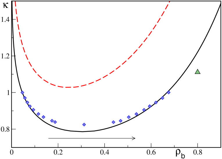
Figure 1: Phase diagram for $\alpha=1.8$. Standard mean-field theory (broken red like), BH theory (full black line) and MC simulation data taken from Ref.stell . The triangle indicates the state-point at which we show the radial distribution in Fig.2 and the arrow indicates the path taken when calculating the density profiles in Fig.5.

Test particle

As a first test of the BH functional we will focus on a situation where the external field is a fluid particle fixed at the origin

$$V_{\rm ext}(r)=\begin{cases}\hskip 25.6073pt\infty&r<1,\vspace*{0.2cm}\\ -\kappa\,\frac{e^{-\alpha(r-1)}}{r}&r\geq 1.\end{cases}$$ (54)

The significance of this choice is that the inhomogeneous density about a test particle is related to the bulk radial distribution function according to the Percus identity $g(r)=\rho(r)/\rho_{b}$ evans92 and thus provides direct access to bulk thermodynamic quantities. Numerical minimization of the BH functional was performed on a discrete spatial grid with spacing $\Delta r=0.05$ and using 180 Legendre polynomials. We have checked carefully the robustness of the converged density profiles to variations in the choice of these numerical parameters.

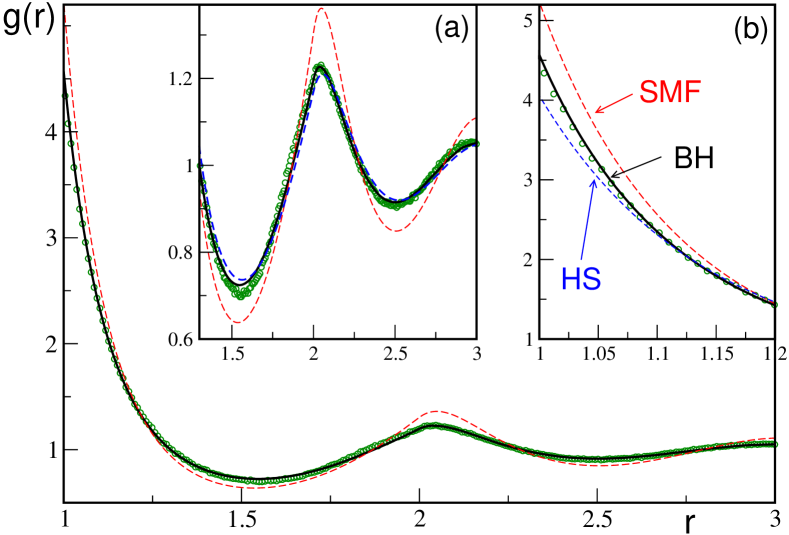
Figure 2: Test particle. Comparison of the radial distribution function calculated using the test particle method with simulation data at $\kappa\!=\!1.111$ and $\rho_{b}=0.8$ (marked with a triangle in Fig.1). Green circles: MC simulation. Full black line: BH functional. Broken red line: SMF theory. Dashed blue line: The density of pure hard-spheres ($\kappa\!=\!0$, $\rho_{b}\!=\!0.8$) calculated using the Rosenfeld functional. Insets (a) and (b) focus on the second peak and contact value, respectively.

In Fig.2 we compare $g(r)$ calculated using the SMF and the BH theories with MC data for the statepoint at $\kappa=1.111$ and $\rho_{b}=0.8$ (indicated by the triangle in Fig.1). We find that the SMF significantly overestimates the structure in $g(r)$ compared to the simulation. The first (contact) peak is around $16$% too high and the amplitude of subsequent oscillations is too large. These features are consistent with the findings of Archer et al. chacko , who assessed the performance of the SMF in one-dimensional test particle calculations using an exactly solvable model as a benchmark. The BH theory provides an accurate description of the simulation data, showing only small errors in the contact value and depth of the first minimum. It is interesting to note that, despite the large value of $\kappa$, the BH $g(r)$ is very similar to that of pure hard-spheres (also shown in Fig.2). This observation validates a posteriori the van der Waals picture that repulsive interactions dictate the microstructure and is consistent with the perturbation approximation at the heart of BH theory.

On the level of the Euler-Lagrange equation (16) the difference between the SMF and the BH theories is due to the direct correlation contributions $c^{(1)}_{\rm corr}$ and $c^{(1)}_{\rm der}$, which we show in Fig.3. Given the structural overestimation of the SMF theory, these self-consistently determined functions apparently serve to counteract the term $c^{(1)}_{\rm smf}$ and thus yield a radial distribution function very similar to that of hard-spheres. Although the oscillations in $c^{(1)}_{\rm corr}$ and $c^{(1)}_{\rm der}$ are not in phase with each other, the peaks and troughs act to suppress the exaggerated oscillations occuring in the SMF theory. We also observe that both contributions are of comparable magnitude; neglecting $c^{(1)}_{\rm der}$, which would be highly desirable from a computational standpoint, is therefore not a viable option.

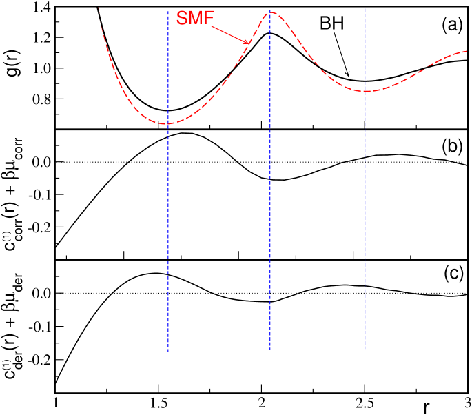
Figure 3: Test particle. The companion to Fig.2 showing the individual contributions to the one-body direct correlation function appearing in equation (16). Full black lines: BH functional. Broken red line: SMF theory. The blue lines are a guide for the eye to show how the maxima and minima of these functions match up with the oscillations in the radial distribution function.

Planar slit

We next consider the density of the HCY fluid confined between two hard-walls separated by a distance $L$ and oriented perpendicular to the $z$-axis. The external potential is given by

$$V_{\rm ext}(z)=\begin{cases}\hskip 1.9919pt0&\frac{1}{2}<z<L-\frac{1}{2},\vspace*{0.2cm}\\ \infty&\hskip 7.11317pt{\rm otherwise},\end{cases}$$ (55)

where we recall that the unit of length is taken to be one particle diameter. Numerical results will be presented for the case $L\!=\!10$. The BH functional was minimized on a grid with spacing $\Delta z=0.05$. When employing the Lado discrete Hankel transform (see Ref. lado for details) it is neccessary to specify a cutoff length, $R$, in the plane parallel to the interface and a maximum number of radial grid points located at the zeros of the Bessel function $J_{0}$. We found that using $R\!=\!14$ and $200$ Bessel zeros provided very accurate results. We carefully checked that the converged density profiles were robust with respect to changes in the numerical parameters.

In Fig.4 we show GCMC data together with the density obtained from the SMF and BH theories, respectively. The theoretical results indicated by broken lines and the simulation data points were calculated at $\kappa=0.5$ and chemical potential $\mu=-1$. As we have a confined system we now specify the chemical potential rather than a bulk density, as the latter is no longer well-defined. The BH functional captures the simulation data very well, only slightly underestimating the density at the centre of the gap. In contrast, the SMF functional underestimates this value by around $26$% and provides a generally poor description of the simulation data.

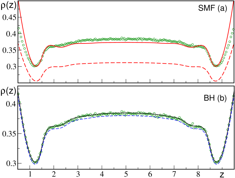
Figure 4: Planar slit. The density between two hard-walls located at $z\!=\!0$ and $10$ for $\kappa\!=\!0.5$. Green circles: GCMC data at $\mu=-1$. DFT profiles calculated at $\mu=-1$ are given by the broken blue line (BH functional) and the broken red line (SMF functional). DFT profiles calculated by adjusting $\mu$ such that the average number of particles in the system matches that of simulation are given by the full black line (BH functional) and the full red line (SMF functional).

The situation discussed above, for which calculations are performed at the same chemical potential as the GCMC simulations, is the correct way to test the quality of an approximate DFT; first-principles predictions are made and then tested. An important factor in determining the form of the density profile is the proximity of the chosen state point to bulk phase coexistence. However, if one wishes to use a given DFT approximation to fit existing simulation (or indeed experimental) data, then better results can be obtained by treating $\mu$ as an optimization parameter. The chemical potential can be tuned such that the average number of particles in the system (i.e. the integral of the density profile) from theory matches that from simulation. The full curves shown in Fig.4 are the result of such a fitting procedure. For the BH functional the chemical potential need only be tuned away from the simulation value ($\mu=\!-1$) by around $1$% to match the average particle number, resulting in a very close fit. In contrast, the SMF theory requires much more substantial adjustment of $\mu$ and, even then, the resulting fit is not satisfactory. We see here, consistent with Fig.2, that the SMF theory tends to overestimate the structure of the density profile, particularly in regions close to a strongly repulsive boundary.

In Fig.5 we show density profiles calculated at $\kappa\!=\!0.75$ for five different values of the chemical potential. As a rule-of-thumb, if we consider the density at the centre of the gap to determine an effective bulk density, then tuning $\mu$ would correspond to following the path indicated in Fig.1. For each of the five statepoints we show both the density profiles calculated at the same chemical potential as used in simulation (broken lines) and those calculated using the fitting procedure described above (full lines). We omit to show results from the SMF functional, because these lie so far from the simulation data that they would only serve to confuse the figure. For the states at $\mu\!=\!-1$ and $\mu\!=\!-1.5$ the BH functional performs very well. The density generated at the true chemical potential already gives a good account of the simulation data and only a very slight tuning of $\mu$ is required to create an excellent fit. This provides further evidence, in addition to the data shown in Fig.2, that the fundamental assumption of the BH theory is accurate for inhomogeneous fluids at high densities.

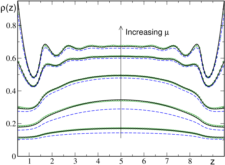
Figure 5: Planar slit. The density between two hard-walls located at $z\!=\!0$ and $10$ for $\kappa\!=\!0.75$. Green circles: GCMC data at chemical potentials $\mu=-2.50,-2.25,-2.00,-1.50$ and $-1.00$ (moving along the arrow marked in Fig.1). Broken blue line: BH functional at the same chemical potentials as used in the simulation. Full black line: BH functional profiles calculated by adjusting $\mu$ such that the average number of particles in the system matches that of simulation.

Deviations start to emerge as $\mu$ is reduced to lower values, reflecting the increasing influence of bulk critical fluctuations. The profile at $\mu\!=\!-2.25$ is the most affected by proximity to the critical point (located at $\mu^{\rm BH}_{\rm crit}\!=\!-2.47$, $\kappa^{\rm BH}_{\rm crit}\!=\!0.79$); the BH theory underestimates the value of the density in the centre of the gap. Nevertheless, for all the considered statepoints tuning $\mu$ still results in a very good fit to the simulation data. This suggests that the structural ‘building blocks’ of the BH functional are sufficient to accurately describe inhomogeneous profiles at all thermodynamic statepoints and that it is rather the bulk thermodynamics which is insufficiently accurate in the critical region. It could be speculated that modifying/tuning the BH functional to have improved bulk thermodynamics, without increasing the structural complexity of the theory, could lead to very accurate results. Such an approach has been successfully applied to the original Rosenfeld hard-sphere functional to ‘upgrade’ the theory from Percus-Yevick to Carnahan-Starling thermodynamics, while retaining the same geometrical weight functions roth .

Free interface

As a final application of the BH functional in planar geometry we consider the free interface between coexisting liquid and gas phases (the densities of which we will denote by $\rho_{\rm l}$ and $\rho_{\rm g}$). The nature of the density profile at the free interface has been the subject of much conjecture, primarily concerning the question of whether the profile exhibits either a monotonic or an oscillatory decay into the bulk. On the gas side of the profile it is established that the decay is monotonic, it is the decay into the bulk liquid which remains the subject of debate.

For model fluids with short-ranged interactions it can be shown that an inhomogeneous density profile ultimately decays into bulk in the same way as the radial distribution function of the bulk fluid (see Ref. poles and references therein). For the free interface this implies that if $g(r)$ exhibits damped oscillatory decay at the coexisting state-point on the liquid side of the binodal, then the corresponding liquid-vapour density profile will decay into the bulk liquid with the same frequency and decay length. The range of $\rho_{\rm l}$ values over which this oscillatory behavior can occur is determined by the point at which the binodal intersects the so-called Fisher-Widom line (a line in the ($\rho_{\rm b},\kappa$) plane marking the cross-over from monotonic to asymptotic decay of $g(r\!\rightarrow\!\infty)$) fisherwidom . One thus arrives at a picture in which a portion of the liquid-side of the binodal, between the triple point and the Fisher-Widom intersection point, should in principle be associated with oscillatory liquid-vapour profiles.

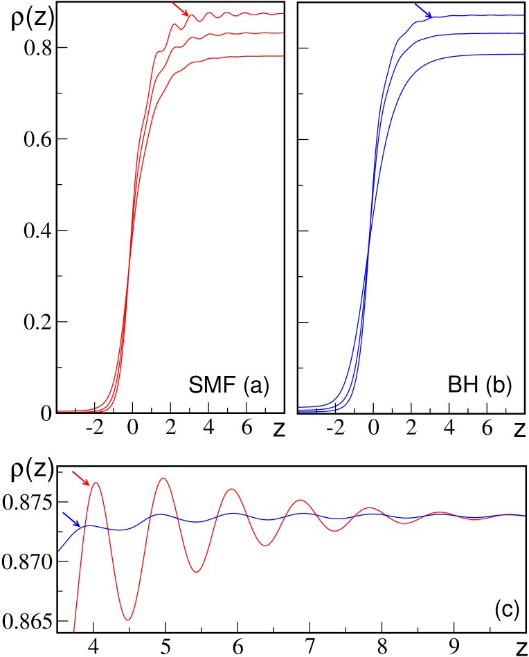
Figure 6: Free interface. Density profiles at the liquid-vapour interface from (a) the SMF functional and (b) the BH functional. As the two theories have different binodals (see Fig.1) we compare profiles with equal values of the coexisting liquid density. Panel (c) focuses on the decay of the density into the bulk liquid for the statepoint closest to the triple-point. The arrows are intended to help the reader better see which of the oscillations in (a) and (b) are being shown in (c).

An important caveat to the above arguments is that the theory of asymptotic decay makes no claim regarding the amplitude of any oscillatory contribution to $\rho(z)$. We can certainly expect any oscillations at the free interface to have smaller amplitude than for solid-fluid interfaces (e.g. the profiles shown in Fig.5) due to the influence of lateral capillary wave fluctuations. Previous DFT investigations have reported oscillatory profiles for a variety of model interaction potentials lv1 ; lv2 ; geysermans . However, all of these studies employed the same SMF functional, raising the obvious question of whether the rather large amplitude of the observed oscillations is a generic feature of DFT or an artifact of the SMF approximation. The fact that this question has not really been addressed is a consequence of both the simplicity with which the SMF functional can be implemented and the lack of alternative approaches; in a sense the term ’density functional study’ has become almost synonymous with ’standard mean-field study’. For this reason the BH functional is of special value, providing the first opportunity to test in some kind of systematic way the robustness of the SMF predictions.

In Fig.6 we show liquid-vapour profiles obtained from both the SMF and the BH functionals for values of $\kappa$ approaching the triple point. We refrain from presenting simulation data as this would require extensive computation beyond the scope of the present work (Ref. lv_sim gives some insight into the difficulties of simulating the free interface). As the two theories have quite different binodals care is required to ensure a fair comparison between the SMF and the BH density profiles. If we restrict our attention to states approaching the triple point (for which $\rho_{\rm l}-\rho_{\rm g}\approx\rho_{\rm l}$), then a reasonable comparison can be achieved by comparing profiles with equal values of $\rho_{\rm l}$. The SMF functional predicts the onset of an oscillatory profile as the triple point is approached, consistent with previous reports lv1 ; lv2 ; geysermans . The statepoint with the highest value of $\rho_{\rm l}$ exhibits well developed oscillatory decay into the bulk with deviations $(\rho(z)-\rho_{\rm l})/\rho_{\rm l}$ on around the $1$% level. The amplitude of these oscillations rapidly diminishes as the value of $\kappa$ is reduced towards the critical point. The corresponding profiles calculated using the BH functional also show oscillatory decay as the triple point is approached, however, the amplitude is strongly reduced with respect to the SMF predictions. This is consistent with our preceeding test particle and planar-slit calculations, which revealed that the overestimation of attraction-induced layering structure in the SMF is systematically corrected by the BH theory. In addition, at equality of $\rho_{\rm l}$ the interfacial width predicted by the BH approximation is somewhat larger than that from the SMF functional. This observation, taken together with the reduced oscillation amplitude, suggests that the BH theory more accurately incorporates the influence of interfacial capillary wave fluctuations than the SMF theory, as we shall discuss below. For a careful discussion of the amplitudes and damping of oscillations at the free interface we direct the reader to Ref. brader_AO .

The development of a microscopic theory for the free interface has been a subject of renewed interest capillary2 ; resonances . One point of progress has been the clarification of the relationship between the van der Waals/DFT picture, based on the density profile, and the capillary wave approach focused on mesoscopic fluctuations of the liquid surface mandelstam ; capillary1 . DFT calculations for this problem generate one-dimensional density profiles that are completely independent of the interfacial area, $A_{\rm xy}$. However, computer simulation studies have shown that the free interface profile clearly depends on the lateral size of the simulation box, such that the profile should be considered as having a parametric dependence, $\rho(z)\rightarrow\rho(z;A_{\rm xy})$ lv_sim ; capillary1 . A possible resolution of this apparent contradiction is that an approximate mean-field DFT only incorporates the influence of capillary-wave fluctuations up to a certain effective cutoff distance, $\lambda_{\rm DFT}$, within the plane of the interface. This provides the appealing physical picture that mean-field DFT theories are comparable to finite-size simulations, except that within DFT the ‘box size’ is hard-wired by the specific approximation employed. Unfortunately, a precise statistical mechanical definition of $\lambda_{\rm DFT}$ seems to be lacking at present.

In the absence of gravity it is well-known that mean-field theory predicts a divergent transverse correlation length within the interface evans92 . The fact that the derivative of the density profile, $d\rho(z)/dz$, remains nonvanishing indicates that the mean-field approximation does not sufficiently incorporate the feedback of the long-ranged transverse correlations into the density profile. Our interpretation of the difference between the SMF and the BH profiles shown in Fig.6 is thus that the BH theory provides a better account of the coupling between the one- and two-body correlation functions and thus captures this feedback in a more realistic fashion.

IV Discussion

In this paper we have developed and implemented a first-principles DFT for inhomogeneous fluids with attractive interactions. The theory generalizes the successful BH bulk theory and generates density profiles in quantitative agreement with simulation data, marking a significant improvement over the commonly employed SMF functional. Unlike previous efforts our approach avoids reference to any bulk information and is valid for an arbitrary external field. The lack of an accurate and tractable DFT for treating attractive interactions has been a long-standing hinderance to theoretical progress and we hope that our findings will go some way towards alleviating these difficulties. We have already mentioned the alternative theories most directly related to the BH functional, namely the SMF and effective density approaches averagerho1 ; averagerho2 ; averagerho3 ; averagerho4 ; averagerho5 ; averagerho6 . In the following we would like to discuss some additional approximation schemes which could be regarded as rivals to the inhomogeneous BH theory.

A central feature of the DFT formalism is the dual hierarchy of correlation functions, obtained by functional differentiation of the free energy evans92 . Differentiation with respect to an external (or interaction) potential generates density correlators, whereas differentiation with respect to the density generates direct correlation functions. The BH functional stems from the former way of thinking and is essentially a functional expansion of the excess free energy in powers of the attractive contribution to the interaction potential. This demands that we have a detailed understanding of a given reference system for any $\rho({\bf r})$, which is indeed the case for hard-spheres. However, the problem can also be approached using the second hierarchy, by performing a functional Taylor expansion of the excess free energy in powers of $\rho({\bf r})$ about a reference density evans79 ; evans92 ; rama ; wu . This requires that for the given reference density we have complete understanding of the fully interacting system, which is generally not the case. For this reason a bulk density is usually chosen as a reference (implicitly assuming a weakly nonuniform fluid) and the Taylor series is truncated at quadratic-order, such that only the bulk pair direct correlation functions are required as input. Although respectable results can be obtained for systems of repulsive particles (especially in the case of soft penetrable particles) the theory is less successful when applied to systems with an attractive component to the interaction potential. In particular, an excess free energy with a quadratic dependence on the density cannot describe two minima and is thus not capable of describing phase transitions at interfaces evans92 .

The sum of all terms beyond quadratic order in the density expansion is known as the ‘bridge functional’ Hansen06 ; attard_book . Rosenfeld has shown that the quadratic functional can be much improved by replacing the true bridge functional of the fully interacting system with that of the hard-sphere system (often referred to as either the ‘reference functional’ or ‘universal bridge functional’ method) rosenfeld_bridge . This approach is somewhat similar in spirit to our inhomogeneous BH theory, for which the total correlation function $h_{\rm hs}({\bf r}_{1},{\bf r}_{2};[\rho])$ is assumed ‘universal’ for any attractive interaction. On the positive side, the universal bridge functional method can make very accurate predictions in certain cases and has the convenient feature that only one-body functions are required rosenfeld_bridge ; oettel ; sweatman1 ; sweatman2 . However, compared with the BH functional we observe two fundamental disadvantages of the Bridge functional approach: (i) Despite resumming higher order terms, the theory is still a density expansion and thus cannot escape the need to identify a bulk reference state. This is problematic for confined fluids. (ii) To yield accurate results the hard-sphere reference functional has to be evaluated at some effective hard-sphere diameter. This introduces a free parameter for which an optimization criterion must be specified. In our view, the assumption that $h_{\rm hs}({\bf r}_{1},{\bf r}_{2};[\,\rho\,])$ is ‘universal’ constitutes a physically clear generalization of van der Waals vision of the liquid state, whereas the universal bridge functional seems to be a more obscure formal object.

An alternative to the aforementioned DFT approximations is to attack the pair correlations directly by applying an inhomogeneous closure to the OZ equation (e.g. hypernetted-chain) for the full interaction potential attard_book . While integral equation theories can provide accurate results (see Refs. attard1 ; shoulder ; kovalenko for example) they suffer from the following well-known problems: (i) There exist ‘no-solution’ regions in thermodynamic parameter-space where the theory fails to converge. In the case of liquid-gas phase separation this region typically envelopes the critical point and thus prevents both a proper determination of the binodal and the investigation of any associated interfacial phenomena. (ii) Thermodynamic inconsistency. Making an approximation on the level of the pair correlations, rather than on the level of the free energy, has the consequence that the density profile is not unique. The three formally exact routes from the pair correlations to the density will yield inconsistent results attard_book . These failings, which are ultimately linked to the absence of a generating (free energy) functional, make inhomogeneous integral equations theories generally unsuitable for the investigation of interfacial phase transitions.

Finally, we would like to outline some possibilities for future work. On the technical side, now that we have established the accuracy of the BH functional it would be worth to invest effort into improving the numerical efficiency of our algorithms. The bottleneck in our calculations is the iterative solution of the OZ equation, which requires a constant back-and-forth between real and transform (either Legendre or Hankel) space. We plan to investigate existing proposals to speed-up these transforms LadoSpeedup as well as the possibility to generalize methods developed for solving the OZ equation in bulk to the inhomogeneous case (see brader_critical and references therein). An alternative method to improve numerical efficiency would be to exploit the analytic expression for $c_{\rm hs}({\bf r}_{1},{\bf r}_{2})$ generated by taking two functional derivatives of the Rosenfeld functional (c.f. equation (23)).

Regarding future physical investigations, the ability of the BH functional to describe accurately systems with an attractive component to the interaction potential could be exploited to address a variety of topics. Some possibilities are: (i) To apply the BH functional to a system interacting via a competing attractive and repulsive interaction (the so-called short-range attractive and long-range repulsive (SALR) class of potential) melascio ; archer_wilding . Standard liquid state theories are unable to account for the complex phase behavior presented by these systems and it would therefore be of interest to investigate the predictions of the BH functional. (ii) There have been recent advances in obtaining canonical observables (i.e. the density profile) from grand-canonical DFT; ensemble differences become important when considering small systems with few particles canonical transform ; canonicalDDFT . Application of this method to realistic systems with attractive interactions has so-far been hindered by the absence of an accurate grand canonical functional. The BH functional could thus open-up possibilities to study, e.g. nucleation and clustering in small systems. (iii) Although technically challenging, it would be interesting to investigate in detail the inhomogeneous two-body correlations within the liquid-vapour interface, with a view to shedding light on the nature of the ‘intrinsic interface’ predicted by mean-field DFT.

Appendix A

Consider the functional derivative of an arbitrary functional $H$ with respect to a scalar function $g({\bf r})$.

$$\frac{\delta H[g]}{\delta g({\bf r})}.$$ (56)

The derivative can be reversed to recover $H$ by the following integration

$$H[g]=H[g_{\rm r}]+\int\!d{\bf r}\int_{g_{\rm r}({\bf r})}^{g({\bf r})}\!d\tilde{g}({\bf r})\frac{\delta H[\tilde{g}]}{\delta\tilde{g}({\bf r})},$$ (57)

where $g_{\rm r}({\bf r})$ is a reference function and $\tilde{g}({\bf r})$ is a dummy integration variable. The integration in (57) is a one-dimensional integral over the value of $\tilde{g}$ at point ${\bf r}$. Provided that the functional $H$ is unique, the result will be independent of the chosen path in function space. The simplest choice is then a linear parametric path

$$\tilde{g}({\bf r})\equiv g_{\alpha}({\bf r})=g_{\rm r}({\bf r})+\alpha(g({\bf r})-g_{\rm r}({\bf r})),$$ (58)

where the ‘charging parameter’ $\alpha$ varies from zero to unity. Equation (57) thus becomes

$$H[g]=H[g_{\rm r}]+\int_{0}^{1}\!\!d\alpha\!\int\!d{\bf r}\,\Delta g({\bf r})\frac{\delta H[g_{\alpha}]}{\delta g_{\alpha}({\bf r})},$$ (59)

where $\Delta g({\bf r})\equiv g({\bf r})-g_{\rm r}({\bf r})$. Generalization to the case of two vector arguments is straightforward:

$$G[f]=G[f_{\rm r}]+\!\int_{0}^{1}\!\!d\alpha\!\int\!d{\bf r}\!\int\!d{\bf r}^{\prime}\,\Delta f({\bf r},{\bf r}^{\prime})\frac{\delta G[f_{\alpha}]}{\delta f_{\alpha}({\bf r},{\bf r}^{\prime})},$$ (60)

where $\Delta f({\bf r},{\bf r}^{\prime})\equiv f({\bf r},{\bf r}^{\prime})-f_{\rm r}({\bf r},{\bf r}^{\prime})$, and we have again assumed a linear integration path.

Appendix B

Our perturbative approach employs the hard-sphere reference free energy functional $F_{\rm hs}=F_{\rm id}+F_{\rm hs}^{\rm exc}$. Within Rosenfeld’s original fundamental measures approach the excess Helmholtz free energy is given by rosenfeld89

$$\beta F^{\rm exc}_{\rm hs}[\,\rho\,]=\int d{\bf r}_{1}\;\Phi\left(\left\{n_{\alpha}({\bf r}_{1})\right\}\right),$$ (61)

where the reduced free energy density is a function of a set of weighted densities

$$\Phi=-n_{0}\ln(1-n_{3})+\frac{n_{1}n_{2}-{\bf n}_{1}\cdot{\bf n}_{2}}{1-n_{3}}+\frac{n_{2}^{3}-3n_{2}{\bf n}_{2}\cdot{\bf n}_{2}}{24\pi(1-n_{3})^{2}}.$$ (62)

The four scalar weighted densities, $n_{0}\cdots n_{3}$, and two vector weighted densities, ${\bf n}_{1}$ and ${\bf n}_{2}$, are given by

$$n_{\alpha}({\bf r}_{1})=\int d{\bf r}_{2}\;\rho({\bf r}_{2})\,\omega_{\alpha}({\bf r}_{1}-{\bf r}_{2}),$$ (63)

where the weight functions, characteristic of the geometry of the hard-spheres with a radius $R$, are given by

$$\omega_{3}({\bf r}) =\Theta(R-r),$$

$$\omega_{2}({\bf r}) =\delta(R-r),$$

$$\boldsymbol{\omega}_{2}({\bf r}) =\frac{{\bf r}}{r}\delta(R-r),$$ (64)

and $\omega_{1}({\bf r})=\omega_{2}({\bf r})/(4\pi R)$, $\omega_{0}({\bf r})=\omega_{2}({\bf r})/(4\pi R^{2})$ and $\boldsymbol{\omega}_{1}({\bf r})=\boldsymbol{\omega}_{2}({\bf r})/(4\pi R)$. The (negative) first functional derivative of the excess free energy yields the one-body direct correlation function

$$c^{(1)}_{\rm hs}({\bf r}_{1})=-\sum_{\alpha}\int d{\bf r}_{2}\frac{\partial\Phi}{\partial n_{\alpha}({\bf r}_{2})}\omega_{\alpha}({\bf r}_{2}-{\bf r}_{1}).$$ (65)

Explicit expressions for $c^{(1)}_{\rm hs}({\bf r}_{1})$ in both planar and spherical geometry can be found in subsections 8.2 and 8.3 of Ref. roth .

Appendix C

For the hard-sphere system both $h_{\rm hs}({\bf r}_{1},{\bf r}_{2})$ and $c_{\rm hs}({\bf r}_{1},{\bf r}_{2})$ are discontinuous when $|{\bf r}_{1}-{\bf r}_{2}|=d$. If these functions are directly transformed then the precise location of the discontinuity becomes uncertain on the order of the numerical grid spacing. Using diagrammatic analysis it can be shown that the function

$$\gamma({\bf r}_{1},{\bf r}_{2})=h({\bf r}_{1},{\bf r}_{2})-c({\bf r}_{1},{\bf r}_{2})$$ (66)

is a continuous function for any interaction potential attard_book . Using equation (66) to eliminate $h_{\rm hs}({\bf r}_{1},{\bf r}_{2})$ from the OZ equation (22) yields an alternative form

$$\gamma_{\rm hs}({\bf r}_{1},{\bf r}_{2}) =\int\!d{\bf r}_{3}\,c_{\rm hs}({\bf r}_{1},{\bf r}_{3})\rho({\bf r}_{3})c_{\rm hs}({\bf r}_{3},{\bf r}_{2})$$

$$+\int\!d{\bf r}_{3}\,\gamma_{\rm hs}({\bf r}_{1},{\bf r}_{3})\rho({\bf r}_{3})c_{\rm hs}({\bf r}_{3},{\bf r}_{2}),$$ (67)

for which we only have to deal with one discontinuous function, namely $c_{\rm hs}$. In spherical geometry a Legendre transformation reduces equation (Appendix C) to an equation for the transforms

$$G_{n}(r_{1},r_{2}) =\frac{4\pi}{2n+1}\Bigg{(}\int_{0}^{\infty}\!\!dr_{3}\,r_{3}^{2}\,C_{n}(r_{1},r_{3})\rho(r_{3})\,C_{n}(r_{3},r_{2}).$$

$$+\!\!\int_{0}^{\infty}\!\!dr_{3}\,r_{3}^{2}\,G_{n}(r_{1},r_{3})\rho(r_{3})\,C_{n}(r_{3},r_{2})\Bigg{)},$$ (68)

where $G_{n}$ is the Legendre transform of $\gamma_{\rm hs}$. In planar geometry a Hankel transform of equation (Appendix C) generates the following simplified form

$$\mathcal{G}_{k}(z_{1},z_{2}) =\int_{-\infty}^{\infty}\!\!dz_{3}\,\mathcal{C}_{k}(z_{1},z_{3})\rho(z_{3})\mathcal{C}_{k}(z_{3},z_{2})$$

$$+\int_{-\infty}^{\infty}\!\!dz_{3}\,\mathcal{G}_{k}(z_{1},z_{3})\rho(z_{3})\mathcal{C}_{k}(z_{3},z_{2}),$$ (69)

where $\mathcal{G}_{k}$ is the Hankel transform of $\gamma_{\rm hs}$. The general equation (II) for the perturbed pair correlations as well as the reduced forms for spherical and planar geometry, equations (II) and (II), respectively, can also be rewritten in the alternative form by trivial extension of the above expressions.

Equations (Appendix C) and (Appendix C) both require a discrete integral transform of the discontinuous pair direct correlation function. However, the analogous procedure for the Hankel transform has not been documented. Defining a critical radius $R_{\rm c}=(d^{2}-(z_{1}-z_{2})^{2})^{\frac{1}{2}}$ we can at any time in the iterative cycle use the continuous function $\gamma_{\rm hs}$ to evaluate both the direct correlation function

$$c_{\rm hs}(z_{1},z_{2},R_{\rm c}) =-1-\gamma_{\rm hs}(z_{1},z_{2},R_{\rm c})$$

$$=c_{\rm st}(z_{1},z_{2}),$$ (70)

and the derivative

$$\frac{\partial c_{\rm hs}(z_{1},z_{2},\bar{r}_{12})}{\partial\bar{r}_{12}}{\bigg{|}}_{R_{\rm c}} =-\frac{\partial\gamma_{\rm hs}(z_{1},z_{2},\bar{r}_{12})}{\partial\bar{r}_{12}}{\bigg{|}}_{R_{\rm c}}$$

$$=c_{\rm sl}(z_{1},z_{2}).$$ (71)

We then use these quantities to define the following linear step function

$$f(z_{1},z_{2},\bar{r})=\begin{cases}c_{\rm st}+c_{\rm sl}(\bar{r}-R_{c}),&\bar{r}<R_{c}\\ \hskip 15.6491pt0,&\bar{r}>R_{c}\end{cases}$$ (72)

which will allow us to remove the unwanted discontinuity. The analytical Hankel transform of equation (72) is given by

$$\overline{f}(k) =c_{\rm st}\frac{2\pi R_{c}}{k}J_{1}(kR_{c})$$ (73)

$$-c_{\rm sl}\Bigg{(}\frac{\pi^{2}R_{c}}{k^{2}}\Big{(}J_{1}(kR_{c})S_{0}(kR_{c})-J_{0}(kR_{c})S_{1}(kR_{c})\Big{)}\Bigg{)},$$

where $S_{0}$ and $S_{1}$ are the zeroth and first-order Struve functions, respectively. Thus, to numerically Hankel transform $c_{\rm hs}$ we perform the following steps: (i) Construct the continuous and smooth function $\alpha=c_{\rm hs}\!-\!f$, (ii) Numerically transform to obtain $\bar{\alpha}$, (iii) Add the analytic transform, $\bar{c}_{\rm hs}=\bar{\alpha}+\bar{f}$. To perform the inverse transform we simply reverse this procedure: (i) Construct $\bar{\alpha}=\bar{c}_{\rm hs}-\bar{f}$, (ii) Numerically inverse transform to get $\alpha$, (iii) Add the linear step, $c_{\rm hs}=\alpha+f$. Using these techniques the numerical transform is at no point confronted with a discontinuous function. An analogous treatment of the Legendre transform for the case of spherical symmetry is described in the Appendix of Ref. attard1 .

References

- (1) J.D. van der Waals, thesis, Univ. Leiden (1873).
- (2) L. Boltzmann, Lectures on Gas Theory (translated by S.G. Brush), (Berkeley, 1964).
- (3) L.S. Ornstein and F. Zernike, Proc. Acad. Sci. Amst., 17, 793 (1914).
- (4) M. Kac, G.E. Uhlenbeck and P.C. Hemmer, J. math. Phys., 4, 216, 229 (1963); M. Kac, G.E. Uhlenbeck and P.C. Hemmer, J. math. Phys., 5, 60 (1964).
- (5) R.W. Zwanzig, J. Chem. Phys. 22, 1420, (1954).
- (6) J.K. Percus and G.J. Yevick, Phys. Rev. 110, 1 (1958).
- (7) M.S. Wertheim, Phys. Rev. Lett. 10 321 (1963).
- (8) E. Thiele, J. Chem. Phys. 39, 474 (1963).
- (9) W. R. Smith and D. Henderson, Mol. Phys. 19, 411 (1970).
- (10) J. A. Barker and D. Henderson, J. Chem. Phys., 47, 2856 (1967).
- (11) J. A. Barker and D. Henderson, J. Chem. Phys., 47, 4714 (1967).
- (12) J. A. Barker and D. Henderson, Rev. Mod. Phys. 48, 587 (1976).
- (13) J. S. Høye and G. Stell, J. Chem. Phys., 67 439 (1977).
- (14) D. Pini, G. Stell and N. B. Wilding, Mol. Phys., 95, 483 (1998).
- (15) A. Parola and L. Reatto, Phys. Rev. Lett. 53 2417 (1984); A. Parola and L. Reatto, Phys. Rev. A 31 3309 (1985).
- (16) J. P. Hansen and I. R. McDonald, Theory of Simple Liquids, 3rd ed. (Academic Press, London, 2006).
- (17) R. Evans, Adv. Phys. 28, 143 (1979).
- (18) R. Evans, Density functionals on the theory of nonuniform fluids. In Fundamentals of Inhomogeneous Fluids, Edited by D. Henderson (Dekker, New York 1992).
- (19) M. H. Kalos, J. K. Percus and M. Rao, J. Stat. Phys., 17, (1977).
- (20) S. Sokolowski and J. Fischer, J. Chem. Phys. 96, 5441 (1992).
- (21) J. C. Barrett, J. Chem. Phys. 124, 144705 (2006).
- (22) P. Lurie-Gregg, J. B. Schulte and D. Roundy, Phys. Rev. E 90 042130 (2014).
- (23) Z. Tang, L.E. Scriven and H.T. Davis, J. Chem. Phys. 95 2659 (1991).
- (24) S. Varga, D. Boda, D. Henderson and S. Sokolowski, J. Colloid and Interface Science, 227 223 (2000).
- (25) A. J. Archer, B. Chacko and R. Evans, J. Chem. Phys. 147, 034501 (2017)
- (26) J. M. Brader and M. Schmidt Mol. Phys. 113 2873 (2015).
- (27) D.E. Sullivan, Phys. Rev. A 25 1669 (1982).
- (28) H.C. Anderson, D. Chandler and J.D. Weeks, J.Chem.Phys. 56 3812 (1972).
- (29) B. D. Kelly, W. R. Smith and D. Henderson, Mol. Phys. 114, 2446 (2016).
- (30) Y. Rosenfeld, Phys. Rev. Lett. 63 980 (1989).
- (31) R. Roth, J.Phys.:Condens.Matter 22 063102 (2010).
- (32) P. Attard, Thermodynamics and statistical mechanics: Equilibrium by Entropy Maximisation (Elsevier, (2002)).
- (33) P. Attard, J. Chem. Phys. 91, 3072 (1989).
- (34) M.P. Allen and D. J. Tildesley, Computer simulation of liquids (Oxford university press, (2017)).
- (35) F. Lado, J. Comp. Phys. 8 417 (1971).
- (36) Simulations of the full phase diagram for values of have been performed by L. Mederos and G. Navascuéz, J. Chem. Phys. 101, 9841 (1994). Extrapolation of their data allows us to roughly estimate the triple point density for .
- (37) R. Evans, R. J. F. Leote de Carvalho, J. R. Henderson and D. C. Hoyle, J. Chem. Phys. 100, 591 (1994).
- (38) M.E. Fisher and B. Widom, J. Chem. Phys. 50, 3756 (1969).
- (39) R. Evans, J. R. Henderson, D. C. Hoyle, A. O. Parry and Z. A. Sabeur, Mol. Phys. 80 755 (1993).
- (40) R. Checa, E. Chacón and P. Tarazona, Phys. Rev. E 70 061601 (2004).
- (41) P. Geysermans, N. Elyeznasni and V. Russier, J. Chem. Phys. 123, 204711 (2005).
- (42) P. Tarazona, E. Chacón, M. Reinaldo-Falagán and E. Velasco, J. Chem. Phys. 117 3941 (2002).
- (43) J.M. Brader, R.Evans and M.Schmidt, Mol.Phys. 101 (23-24), 3349 (2003)
- (44) E.M. Fernández E. Chacón, P. Tarazona, A.O. Parry and C. Rascón, Phys. Rev. Lett. 111 096104 (2013).
- (45) A.O. Parry and C. Rascón, Nature Physics 15 287 (2019).
- (46) J.S. Rownlinson and B. Widom, Molecular Theory of Capillarity (Oxford: Clarendon).
- (47) P. Tarazona, E. Chacón and F. Bresme, J. Phys.: Condens. Matter 24 284123 (2012).
- (48) T. Ramakrishnan and M. Yussouff, Phys. Rev. B 19 2775 (1979).
- (49) Y. Tang and J. Wu, Phys. Rev. E 70 011201 (2004).
- (50) Y. Rosenfeld, J. Chem. Phys. 98, 8126 (1993).
- (51) M. Oettel, J. Phys.: Condens. Matter 17 429 (2005).
- (52) M.B. Sweatman, PhD thesis, University of Bristol, UK, (1995).
- (53) M.B. Sweatman, Mol. Phys. 98, 573 (2000).
- (54) J.M. Brader, J. Chem. Phys. 128, 104503 (2008).
- (55) I. Omelyan, F. Hirata and A. Kovalenko, Phys. Chem. Chem. Phys., 7, 4132 (2005).
- (56) F. Lado, Mol. Phys. 107 301 (2009).
- (57) J.M. Brader, International Journal of Thermophysics 27, 394 (2006).
- (58) G. Melascio, J. Phys. Condens. Matter 19 073101 (2007).
- (59) A.J. Archer and N.B. Wilding, Phys. Rev. E, 76, 031501 (2007).
- (60) U.M.B. Marconi and P. Tarazona, J. Chem. Phys. 110, 8032 (1999).
- (61) D. de las Heras, and M. Schmidt Phys. Rev. Lett., 113, 238304, (2014).
- (62) T. Schindler, R. Wittmann and J.M. Brader, Phys.Rev.E 99 012605 (2019).