Ordered ground states of kagome magnets with generic exchange anisotropy

Abstract

There is a growing family of rare-earth kagome materials with dominant nearest-neighbor interactions and strong spin orbit coupling. The low symmetry of these materials makes theoretical description complicated, with six distinct nearest-neighbor coupling parameters allowed. In this Article, we ask what kinds of classical, ordered, ground states can be expected to occur in these materials, assuming generic (i.e. non-fine-tuned) sets of exchange parameters. We use symmetry analysis to show that there are only five distinct classical ground state phases occurring for generic parameters. The five phases are: (i) a coplanar, 2-fold degenerate, state with vanishing magnetization (${\sf A_{1}}$), (ii) a noncoplanar, 2-fold degenerate, state with magnetization perpendicular to the kagome plane (${\sf A_{2}}$), (iii) a coplanar, 6-fold degenerate, state with magnetization lying within the kagome plane (${\sf E}$-coplanar), (iv) a noncoplanar, 6-fold degenerate, state with magnetization lying within a mirror plane of the lattice (${\sf E}$-noncoplanar₆), (v) a noncoplanar, 12-fold degenerate, state with magnetization in an arbitrary direction (${\sf E}$-noncoplanar₁₂). All five are translation invariant (${\bf q}=0$) states. Having found the set of possible ground states, the ground state phase diagram is obtained by comparing numerically optimized energies for each possibility as a function of the coupling parameters. The state ${\sf E}$-noncoplanar₁₂ is extremely rare, occupying $<1\%$ of the full phase diagram, so for practical purposes there are four main ordered states likely to occur in anisotropic kagome magnets with dominant nearest neighbor interactions. These results can aid in interpreting recent experiments on “tripod kagome” systems R₃A₂Sb₃O₁₄, as well as materials closer to the isotropic limit such as Cr- and Fe- jarosites.

I Introduction

Frustration can come from various sources. This is certainly true of the frustration exhibited by many magnetic materials, which may be generated by the geometry of the lattice Ramirez (1994); Harris et al. (1997), by competition between interactions of different kinds Henley (1989); Iqbal et al. (2019) or by bond-dependent anisotropies Kitaev (2006); Rousochatzakis and Perkins (2017). Sometimes, all of these sources of frustration are present at once, making the problem of determining a ground state both more challenging and more rich Yan et al. (2017); Essafi et al. (2017); Zhu et al. (2018).

Kagome lattice rare-earth materials Zorko et al. (2010); Ghosh et al. (2014); Sharma et al. (2016); Sanders et al. (2016a, b); Dun et al. (2016); Scheie et al. (2016); Dun et al. (2017); Scheie et al. (2018); Ding et al. (2018); Scheie et al. (2019) provide a realization of this scenario. The kagome lattice [Fig. 1] is paradigmatic of geometrical frustration while the strong spin-orbit coupling inherent to many rare-earth ions produces complicated anisotropic exchange interactions with distinct, competing, contributions and bond-dependence.

In this Article we study a model of anisotropic exchange on the kagome lattice, including all possible nearest neighbor interactions consistent with the lattice symmetries Essafi et al. (2017). This model has six independent coupling parameters, once one allows for the absence of reflection symmetry in the kagome plane, as is appropriate for many materials.

Several previous works have investigated different types of allowed anisotropic nearest-neighbor interaction on the kagome lattice Essafi et al. (2017); Elhajal et al. (2002); Ballou et al. (2003); Cépas et al. (2008); Messio et al. (2010); Chernyshev and Zhitomirsky (2014); Götze and Richter (2015); Essafi et al. (2016); Changlani et al. (2018); Morita et al. (2018); Yang et al. (2020), but none has treated all possible interactions at once, in the absence of reflection symmetry in the plane. Thus, in some sense, these previous works can be viewed as higher-symmetry limits of the generic case studied here. Our goal in this work is to identify the ordered, classical, ground states which are stable over a finite fraction of the six dimensional parameter space of the full model. We will not address the physics at the phase boundaries between different states or limits featuring high symmetry beyond time reversal and lattice symmetries, or cases of accidental degeneracy, although these can be of interest. In this sense, we are studying those ground states stable in the presence of “generic” exchange anisotropy.

We find that in the full six-dimensional parameter space there are only five such distinct ground states. They are all translationally invariant, and may be classified by how they transform under the $C_{3v}$ point group symmetries of the kagome lattice. Example spin configurations for each are shown in Figs. 2-6.

In addition to materials with strong exchange anisotropy, our approach is also useful for understanding materials where anisotropy is weak but nevertheless plays a key role in selecting the ground state due to the frustrated nature of Heisenberg interactions on the kagome lattice. Our results can be viewed as illuminating the spectrum of possible ground states which can be obtained by perturbing an isotropic kagome magnet with various allowed forms of nearest-neighbor exchange anisotropy. This may be of use in understanding the ordered ground states of materials including the Cr- and Fe- jarosites Grohol et al. (2003); Nishiyama et al. (2003); Morimoto et al. (2003); Matan et al. (2006); Yildirim and Harris (2006) and Cd-kapellasite Okuma et al. (2017).

The remainder of this Article is organised as follows:

• In Section II we review the most general symmetry allowed nearest neighbor exchange Hamiltonian for the kagome lattice Yildirim and Harris (2006); Essafi et al. (2017). We then analyse it in terms of the irreducible representations of the point group $C_{3v}$.

• Building on this symmetry analysis, in Section III, we demonstrate the five forms of magnetic order which may arise from the generic Hamiltonian.

• In Section IV we use numerical calculations to calculate the ground state phase diagram of the generic Hamiltonian, delineating the regions of parameter space covered by each of the five ordered phases.

• In Section V we discuss experimental results on kagome materials in the light of our calculations.

• In Section VI we close with a brief summary and discussion of open directions for future work.

II Hamiltonian and symmetry analysis

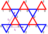
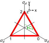
Figure 1: (a) The kagome lattice, a network of corner sharing triangles. The labels $0,1,2$ indicate the convention used to label the three sublattices of the kagome lattice in this work. ${\bf t}_{1}$ and ${\bf t}_{2}$ are the basic translations under which the lattice is symmetric (b) The $C_{3v}$ point group, composed of three reflection symmetries and a threefold rotation axis through the center of the triangle.

We consider generalized bilinear anisotropic exchange interactions on a kagome lattice [Fig. 1],

$$\mathcal{H}=\sum_{\langle ij\rangle}{\bf S}_{i}\cdot{\bf J}_{ij}\cdot{\bf S}_{j}.$$ (1)

We require that the interactions respect the following symmetries:

• Time reversal

• Lattice translations, ${\bf t}_{1},{\bf t}_{2}$, indicated in Fig. 1

• Spatial inversion through lattice sites

• $C_{3}$ rotations around the center of each kagome triangle [Fig. 1]

• Reflections in the mirror planes indicated in Fig. 1

We do not assume any reflection symmetry in the plane of the lattice itself.

We assume that the spins ${\bf S}_{i}$ transform like magnetic moments, i.e. as axial vectors, odd under time reversal symmetry. This will apply not only when ${\bf S}_{i}$ is a true magnetic moment but also when it is a pseudospin-$1/2$ degree of freedom describing the 2-fold degenerate crystal electric field (CEF) ground states of a Kramers ion. In this case the actual magnetic moment is related to the pseudospin via the g-tensor

$${\bf m}_{i}={\bf g}_{i}\cdot{\bf S}_{i}.$$ (2)

An alternative case is possible in which ${\bf S}_{i}$ is a pseudospin describing the low energy CEF states of a non-Kramers ion, which will generally be non-degenerate due to a lack of protection from time reversal symmetry. In the non-Kramers case, the pseudospin operators ${\bf S}_{i}$ will transform differently under time-reversal and the discussion in this section will not apply Onoda and Tanaka (2011); Chen (2019).

We now proceed to constrain the form of the exchange matrices ${\bf J}_{ij}$ using the symmetries listed above. Time reversal symmetry $\mathcal{T}$

$$\mathcal{T}{\bf S}_{i}=-{\bf S}_{i}$$ (3)

is guaranteed by the bilinear form of Eq. (1).

There are three spins in the unit cell, which we label ${\bf S}_{0},{\bf S}_{1},{\bf S}_{2}$ according to the convention in Fig. 1. Translational symmetry imposes that the coupling matrices ${\bf J}_{ij}$ may only depend on which sublattices $i$ and $j$ belong to and whether the bond $ij$ is on an ‘up’ or ‘down’ triangle (red or blue triangles in Fig. 1). Inversion symmetry then guarantees that ‘up’ and ‘down’ triangles have the same coupling matrices.

There are thus three different coupling matrices ${\bf J}_{01},{\bf J}_{12},{\bf J}_{20}$ entering Eq. (1) which define the interactions between nearest neighbour spins on each pair of sublattices.

The form of the matrices ${\bf J}_{ij}$ is constrained by the $C_{3v}$ point group symmetry at the center of each triangle [Fig. 1], and was given in Refs. Essafi et al., 2017; Yildirim and Harris, 2006:

$${\bf J}_{01}=\begin{pmatrix}J_{x}&D_{z}&-D_{y}\\ -D_{z}&J_{y}&K\\ D_{y}&K&J_{z}\\ \end{pmatrix}$$ (4)

$${\bf J}_{12}=$$

$$\begin{pmatrix}\frac{1}{4}(J_{x}+3J_{y})&D_{z}+\frac{\sqrt{3}}{4}(J_{x}-J_{y})&\frac{1}{2}(D_{y}+\sqrt{3}K)\\ -D_{z}+\frac{\sqrt{3}}{4}(J_{x}-J_{y})&\frac{1}{4}(3J_{x}+J_{y})&\frac{1}{2}(\sqrt{3}D_{y}-K)\\ \frac{1}{2}(-D_{y}+\sqrt{3}K)&\frac{1}{2}(-\sqrt{3}D_{y}-K)&J_{z}\\ \end{pmatrix}$$

(5)

$${\bf J}_{20}=$$

$$\begin{pmatrix}\frac{1}{4}(J_{x}+3J_{y})&D_{z}+\frac{\sqrt{3}}{4}(J_{y}-J_{x})&\frac{1}{2}(D_{y}-\sqrt{3}K)\\ -D_{z}+\frac{\sqrt{3}}{4}(J_{y}-J_{x})&\frac{1}{4}(3J_{x}+J_{y})&\frac{1}{2}(-\sqrt{3}D_{y}-K)\\ \frac{1}{2}(-D_{y}-\sqrt{3}K)&\frac{1}{2}(\sqrt{3}D_{y}-K)&J_{z}\\ \end{pmatrix}.$$

(6)

There are six independent parameters in these exchange matrices: three diagonal exchanges $J_{x}$, $J_{y}$, $J_{z}$, two Dzyaloshinskii-Moriya (DM) interactions $D_{y},D_{z}$ and one symmetric off-diagonal exchange $K$.

An additional symmetry which could, in principle, be present is reflection symmetry in the plane of the kagome lattice. The presence of such a symmetry would reduce the set of allowed exchange parameters to four, by setting $D_{y}=K=0$. This case was discussed in detail in Ref. Essafi et al., 2017. In this work, we will continue to assume that there is no reflection symmetry in the kagome plane, as is appropriate for many rare-earth kagome materials Dun et al. (2017). Therefore, we shall take both $D_{y}$ and $K$ to be nonzero.

To begin in determining the phase diagram it is helpful to rewrite the Hamiltonian in terms of objects ${\bf m}_{\gamma,k}$ transforming according to the irreducible representations (irreps) of the point group. ${\bf m}_{\gamma,k}$ are defined for each triangle of the lattice, which we index using $k$. This approach is discussed for the kagome lattice in Ref. Essafi et al., 2017 and the pyrochlore lattice in Ref. Yan et al., 2017.

These objects can function as local order parameters for the different kinds of 3-sublattice order which we will encounter on the phase diagram of the anisotropic exchange model. They also aid in the determination of the phase diagram itself. The appropriate objects are defined in Ref. Essafi et al., 2017 but we reintroduce them here since they are essential to our discussion.

Firstly, there is one scalar object transforming according to the trivial $A_{1}$ representation of $C_{3v}$. A nonzero average value of this field breaks none of the point-group symmetries, only breaking time-reversal symmetry.

$$m_{{\sf A_{1}},k}=\frac{1}{3}\left(\frac{1}{2}S^{x}_{0,k}+\frac{\sqrt{3}}{2}S^{y}_{0,k}+\frac{1}{2}S^{x}_{1,k}-\frac{\sqrt{3}}{2}S^{y}_{1,k}-S^{x}_{2,k}\right)$$

(7)

Here $S^{\alpha}_{i,k}$ is the $\alpha$ component of the spin belonging to sublattice $i$ and triangle $k$.

There are then two linearly independent scalars, which transform according to the $A_{2}$ representation. A nonzero average value of these fields breaks time reversal symmetry and all three mirror symmetries of $C_{3v}$ but preserves the 3-fold rotational symmetry.

$$m_{{\sf A_{2}a},k}=\frac{1}{3}\left(S^{z}_{0,k}+S^{z}_{1,k}+S^{z}_{2,k}\right)$$ (8)

$$m_{{\sf A_{2}b},k}=\frac{1}{3}\left(-\frac{\sqrt{3}}{2}S^{x}_{0,k}+\frac{1}{2}S^{y}_{0,k}+\frac{\sqrt{3}}{2}S^{x}_{1,k}+\frac{1}{2}S^{y}_{1,k}-S^{y}_{2,k}\right)$$

(9)

Finally, there are three two-component vectors, transforming according to the two dimensional E-irrep of $C_{3v}$

$${\bf m}_{{\sf Ea},k}=\frac{1}{3}\begin{pmatrix}S^{x}_{0,k}+S^{x}_{1,k}+S^{x}_{2,k}\\ S^{y}_{0,k}+S^{y}_{1,k}+S^{y}_{2,k}\end{pmatrix}$$ (10)

$${\bf m}_{{\sf Eb},k}=\frac{1}{3}\begin{pmatrix}\frac{1}{2}S^{x}_{0,k}-\frac{\sqrt{3}}{2}S^{y}_{0,k}+\frac{1}{2}S^{x}_{1,k}+\frac{\sqrt{3}}{2}S^{y}_{1,k}-S^{x}_{2,k}\\ -\frac{\sqrt{3}}{2}S^{x}_{0,k}-\frac{1}{2}S^{y}_{0,k}+\frac{\sqrt{3}}{2}S^{x}_{1,k}-\frac{1}{2}S^{y}_{1,k}+S^{y}_{2,k}\end{pmatrix}$$

(11)

$${\bf m}_{{\sf Ec},k}=\frac{1}{3}\begin{pmatrix}\sqrt{\frac{3}{2}}\left(S^{z}_{0,k}-S^{z}_{1,k}\right)\\ \sqrt{2}\left(-\frac{1}{2}S^{z}_{0,k}-\frac{1}{2}S^{z}_{1,k}+S^{z}_{2,k}\right)\end{pmatrix}$$ (12)

In terms of these objects the Hamiltonian may be written

$$\mathcal{H}=\frac{3}{2}\sum_{k}\Bigg{[}\lambda_{\sf A_{1}}m_{{\sf A_{1}},k}^{2}$$

$$\qquad+\left(m_{{\sf A_{2}a},k},m_{{\sf A_{2}b},k}\right)\begin{pmatrix}\lambda_{\sf A_{2},aa}&\frac{\lambda_{\sf A_{2},ab}}{2}\\ \frac{\lambda_{\sf A_{2},ab}}{2}&\lambda_{\sf A_{2},bb}\end{pmatrix}\begin{pmatrix}m_{{\sf A_{2}a},k}\\ m_{{\sf A_{2}b},k}\end{pmatrix}$$

$$\qquad+\left({\bf m}_{{\sf Ea},k},{\bf m}_{{\sf Eb},k},{\bf m}_{{\sf Ec},k}\right)\begin{pmatrix}\lambda_{\sf E,aa}&\frac{\lambda_{\sf E,ab}}{2}&\frac{\lambda_{\sf E,ac}}{2}\\ \frac{\lambda_{\sf E,ab}}{2}&\lambda_{\sf E,bb}&\frac{\lambda_{\sf E,bc}}{2}\\ \frac{\lambda_{\sf E,ac}}{2}&\frac{\lambda_{\sf E,bc}}{2}&\lambda_{\sf E,cc}\end{pmatrix}\begin{pmatrix}{\bf m}_{{\sf Ea},k}\\ {\bf m}_{{\sf Eb},k}\\ {\bf m}_{{\sf Ec},k}\end{pmatrix}\Bigg{]}$$

$$=\frac{3}{2}\sum_{k}\Bigg{[}\lambda_{\sf A_{1}}m_{{\sf A_{1}},k}^{2}+\left(m_{{\sf A_{2}a},k},m_{{\sf A_{2}b},k}\right)\Lambda_{\sf A_{2}}\begin{pmatrix}m_{{\sf A_{2}a},k}\\ m_{{\sf A_{2}b},k}\end{pmatrix}$$

$$\qquad+\left({\bf m}_{{\sf Ea},k},{\bf m}_{{\sf Eb},k},{\bf m}_{{\sf Ec},k}\right)\Lambda_{\sf E}\begin{pmatrix}{\bf m}_{{\sf Ea},k}\\ {\bf m}_{{\sf Eb},k}\\ {\bf m}_{{\sf Ec},k}\end{pmatrix}\Bigg{]}$$ (13)

where $k$ indexes the triangles of the lattice and the final term in Eq. (13) should be interpreted as a sum of 9 scalar products between the vectors ${\bf m}_{{\sf Ei},k}$. The coefficients $\lambda_{\gamma}$ are:

$$\lambda_{\sf A_{1}}=\frac{1}{2}\left(-2\sqrt{3}D_{z}+J_{x}-3J_{y}\right)$$ (14)

$$\lambda_{\sf A_{2},aa}=2J_{z}$$ (15)

$$\lambda_{\sf A_{2},bb}=\frac{1}{2}\left(-2\sqrt{3}D_{z}-3J_{x}+J_{y}\right)$$ (16)

$$\lambda_{\sf A_{2},ab}=2\left(\sqrt{3}D_{y}+K\right)$$ (17)

$$\lambda_{\sf E,aa}=J_{x}+J_{y}$$ (18)

$$\lambda_{\sf E,bb}=\sqrt{3}D_{z}-\frac{J_{x}}{2}-\frac{J_{y}}{2}$$ (19)

$$\lambda_{\sf E,cc}=-J_{z}$$ (20)

$$\lambda_{\sf E,ab}=J_{x}-J_{y}$$ (21)

$$\lambda_{\sf E,ac}=\sqrt{6}D_{y}-\sqrt{2}K$$ (22)

$$\lambda_{\sf E,bc}=\sqrt{8}K$$ (23)

It is then useful to write Eq. (13) in a new basis chosen to diagonalize the matrices $\Lambda_{\sf A_{2}}$ and $\Lambda_{\sf E}$.

$$\mathcal{H}=\frac{3}{2}\sum_{k}\bigg{(}\lambda_{\sf A_{1}}m_{{\sf A_{1}},k}^{2}+\omega_{\sf A_{2}0}m_{{\sf A_{2}0},k}^{2}+\omega_{\sf A_{2}1}m_{{\sf A_{2}1},k}^{2}+$$

$$\qquad\qquad\omega_{\sf E0}{\bf m}_{{\sf E0},k}^{2}+\omega_{\sf E1}{\bf m}_{{\sf E1},k}^{2}+\omega_{\sf E2}{\bf m}_{{\sf E2},k}^{2}\bigg{)}$$ (24)

Here $\omega_{{\sf A_{2}}i}(i=0,1)$ are the eigenvalues of $\Lambda_{\sf A_{2}}$ and $m_{{\sf A_{2}}i}$ are linear combinations of $m_{\sf A_{2}a}$ and $m_{\sf A_{2}b}$ corresponding to the associated eigenvector of $\Lambda_{\sf A_{2}}$ [(Eq. 13)]. Similarly, $\omega_{{\sf E}i}(i=0,1,2)$ are the eigenvalues of $\Lambda_{\sf E}$ and ${\bf m}_{{\sf E}i}$ are linear combinations of ${\bf m}_{\sf Ea}$, ${\bf m}_{\sf Eb}$ and ${\bf m}_{\sf Ec}$ corresponding to the associated eigenvector of $\Lambda_{\sf E}$. We define, without loss of generality,

$$\omega_{\sf A_{2}0}\leq\omega_{\sf A_{2}1},\quad\omega_{\sf E0}\leq\omega_{\sf E1}\leq\omega_{\sf E2}$$ (25)

In this work we will treat the spins as classical vectors of fixed length $|{\bf S}_{i}|=1$. Due to this condition, the following constraint applies to fields ${\bf m}_{\gamma}$ defined in Eqs. (7)-(12):

$$\sum_{\gamma}|{{\bf m}_{\gamma,k}}|^{2}=1,\forall\ k$$ (26)

Eq. (26) is a necessary but not sufficient condition for the proper normalisation of the spins.

It should be emphasised that the reformulation of the problem in terms of variables ${\bf m}_{\gamma,k}$ does not require any further assumptions beyond the nearest-neighbor bilinear, nature of the interactions and the symmetries enumerated at the beginning of this section.

In what follows we will seek to find the classical ground states of Eq. (1).

III What kinds of classical ground state are possible?

In this section we seek to establish the possible classical ordered phases which may occur on the ground state phase diagram of Eq. (1). Our focus is on classical ground states which are stable over finite regions of the full 6-dimensional parameter space. So, although there may be additional ground states which become relevant in particular high symmetry limits of Eq. (1), these are not the subject of our present discussion as they rely on fine-tuning of parameters.

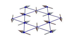
Figure 2: ${\sf A_{1}}$ ordered state, occurring as the ground state of Eq. (1) when $\lambda_{\sf A_{1}}<\omega_{{\sf A_{2}}0},\omega_{{\sf E}0}$ [Eq. (24)]. All spins lie in the kagome plane at an angle of $\frac{2\pi}{3}$ to one another and perpendicular to the line joining the spin to the centers of the two neighboring triangles. The spin configuration has vanishing total magnetization, twofold degeneracy, and preserves the lattice symmetries of Eq. (1) while breaking time reversal.

Our conclusions may be summarized as follows:

1. A translation invariant (${\bf q}=0$) ground state exists for all values of exchange parameters.

2. If

   $$\lambda_{\sf A_{1}}<\omega_{{\sf A_{2}}0},\omega_{{\sf E}0}$$ (27)

   the ground state is the antiferromagnetic state shown in Fig. 2 and discussed in Section III.2.

3. If

   $$\omega_{{\sf A_{2}}0}<\lambda_{\sf A_{1}},\omega_{{\sf E}0}$$ (28)

   the ground state is the noncoplanar state, with magnetization perpendicular to the plane, shown in Fig. 3 and discussed in Section III.3.

4. If

   $$\omega_{{\sf E}0}<\lambda_{\sf A_{2}},\omega_{A_{1}}$$ (29)

   the ground state may be one of three states (${\sf E}$-coplanar, ${\sf E}$-noncoplanar₆, ${\sf E}$-noncoplanar₁₂ ) shown in Figs. 4-6 and discussed in Section III.4.

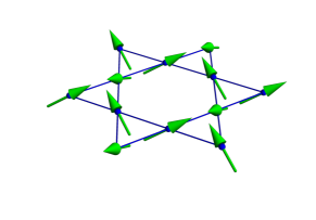
Figure 3: ${\sf A_{2}}$ ordered state, occurring as the ground state of Eq. (1) when $\omega_{{\sf A_{2}}0}<\lambda_{\sf A_{1}},\omega_{{\sf E}0}$ [Eq. (24)]. The spin configuration has magnetization perpendicular to the kagome plane, twofold degeneracy, and breaks the reflection and time reversal symmetries of Eq. (1).

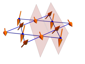
Figure 4: ${\sf E}$-coplanar ordered state. This occurs as a ground state of Eq. (1) in part of the region where $\omega_{{\sf E}0}<\lambda_{\sf A_{1}},\omega_{{\sf A_{2}}0}$ [Eq. (24)]. There is one spin lying in the kagome plane and two canted out of it in such a way that the three spins remain coplanar, with the plane of coplanarity being tilted with respect to the kagome plane. The plane of coplanarity is indicated by the translucent red planes. There is a net magnetization within the kagome plane. This state breaks time reversal and all of the point group symmetries of the Hamiltonian, apart from a single reflection symmetry which is preserved. It is sixfold degenerate.

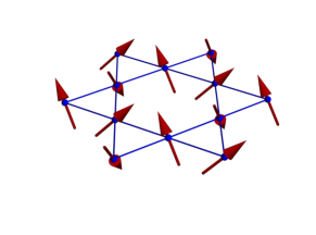
Figure 5: ${\sf E}$-noncoplanar₆ ordered state. This occurs as a ground state of Eq. (1) in part of the region where $\omega_{{\sf E}0}<\lambda_{\sf A_{1}},\omega_{{\sf A_{2}}0}$ [Eq. (24)]. All spins are canted out of the kagome plane and there is a net magnetization lying within one of the mirror planes of the lattice. This state is non-coplanar and thus has nonzero scalar spin chirality. This state breaks time reversal and all of the point group symmetries of the Hamiltonian, but is symmetric under the combination of time reversal and one reflection symmetry. It is sixfold degenerate.

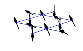
Figure 6: ${\sf E}$-noncoplanar₁₂ ordered state. This occurs as a ground state of Eq. (1) in part of the region where $\omega_{{\sf E}0}<\lambda_{\sf A_{1}},\omega_{{\sf A_{2}}0}$ [Eq. (24)] This state is generally non-coplanar and breaks time reversal symmetry, all point group symmetries and all combinations of time reversal with point group symmetries. It is twelvefold degenerate. This very low symmetry configuration is rare on the ground state phase diagram, occupying $<1\%$ of the full parameter space of the Hamiltonian [Fig. 11].

A summary of the five phases in terms of the values of local order parameters ${{\bf m}_{\gamma}}$ [Eqs. (7)-(12)] is given in Table 1.

In what follows we will demonstrate these results.

Phase	$m_{\sf A_{1}}$	$m_{\sf A_{2}a}$	$m_{\sf A_{2}b}$	$m_{\sf Ea}$	$\psi_{a}$	$m_{\sf Eb}$	$\psi_{b}$	$m_{\sf Ec}$	$\psi_{c}$
${\sf A_{1}}$	$\neq 0$	0	0	0	–	0	–	0	–
${\sf A_{2}}$	$0$	$\neq 0$	$\neq 0$	0	–	0	–	0	–
${\sf E}$-coplanar	$\neq 0$	0	0	$\neq 0$	$\frac{n\pi}{3}$	$\neq 0$	$\frac{n\pi}{3}$	$\neq 0$	$\frac{n\pi}{3}$
${\sf E}$-noncoplanar6	0	$\neq 0$	$\neq 0$	$\neq 0$	$\frac{(2n+1)\pi}{6}$	$\neq 0$	$\frac{(2n+1)\pi}{6}$	$\neq 0$	$\frac{(2n+1)\pi}{6}$
${\sf E}$-noncoplanar12	$\neq 0$	$\neq 0$	$\neq 0$	$\neq 0$	$[0,\pi)$	$\neq 0$	$[0,\pi)$	$\neq 0$	$[0,\pi)$

Table 1: Description of the five possible classical ground states in terms of the local order parameters defined for a triangle in Eqs. (7)-(12). ${\sf E}$ order parameters ${\bf m}_{\sf E_{\alpha}}$ are expressed in polar form, with $m_{\sf E_{\alpha}}$ and $\psi_{\alpha}$ as defined in Eqs. (39)-(41). $n$ is an integer, with different choices of $n$ corresponding to different degenerate ground states in ${\sf E}$-coplanar and ${\sf E}$-noncoplanar₆ phases.

III.1 Existence of ${\bf q}=0$ classical ground state for all parameter sets

Here, for completeness, we give the proof that Eq. (1) possesses a ${\bf q}=0$ classical ground state for all values of exchange parameters, following arguments previously given in Refs. Essafi et al., 2017; Yan et al., 2017. We follow a strategy of building up the global ground state from the ground states of corner sharing units, as is frequently done for models on lattices with a corner-sharing structure Reimers et al. (1991); Essafi et al. (2017); Yan et al. (2017); Morita et al. (2018); Yang et al. (2020).

As we have shown above, the nearest-neighbor exchange Hamiltonian Eq. (1) can be rewritten as a sum over triangles:

$$\mathcal{H}=\sum_{\triangle}\mathcal{H}_{\triangle}$$ (30)

with $\mathcal{H}_{\triangle}$ being the same on every triangle of the lattice, as a consequence of inversion and translation symmetries. This formulation makes it clear that any configuration which minimizes the energy of each individual triangle, also minimizes the energy of the system as a whole.

Such a configuration may readily be obtained by minimizing the energy on a single “up-pointing” triangle (red triangles in Fig. 1) and then tiling the solution over all “up-pointing” triangles of the lattice. The “up-pointing” triangles will then all be in a ground state by construction, and the “down-pointing” triangles will be too, because they have the same exchange matrices as “up-pointing” triangles and the same spin orientation on each sublattice.

This naturally results in a translation invariant (${\bf q}=0$) state, which is guaranteed to be a ground state. Moreover, it means that the ground state problem on the whole lattice can be reduced to finding the ground state of three spins on a triangle.

In Sections III.2-III.4 we examine the various possible solutions to this problem, that occur in different regions of parameter space.

The argument above does not rule out the existence of additional, ${\bf q}\neq 0$, ground states, degenerate with the ${\bf q}=0$ ones. We regard it, however, as unlikely that such accidental degeneracies are present over finite regions of the 6-dimensional parameter space. Such a robust accidental degeneracy, would require a pair of states not related by any symmetry, to be degenerate with respect to each of the six independent terms of the Hamiltonian individually, which would seem to require a rather large coincidence. The Heisenberg-Kitaev model on the kagome lattice Morita et al. (2018); Yang et al. (2020) exhibits an extended, accidental degeneracy, in the classical limit, but since that model only has two symmetry distinct terms the required coincidence is not so large.

From now on, we assume translationally invariant ground states built by tiling the ground states of a single triangle, and therefore drop the triangle index $k$ from the fields ${\bf m}_{\gamma,k}$ and spins ${\bf S}_{i,k}$.

We can use the solutions of the single triangle problem to check the validity of the assumption that there are only ${\bf q}=0$ ground states. We do this by checking whether two distinct single triangle ground states can be placed on neighboring triangles without causing an inconsistency at the shared site. If they cannot, then only ${\bf q}=0$ ground states are possible. This is explicitly checked for each single triangle ground state below, and in each case we find that ${\bf q}\neq 0$ states are only possible with fine tuning.

III.2 $\sf A_{1}$ order

We first consider the parameter regime defined by inequality (27) where $\lambda_{\sf A_{1}}$ is the lowest coefficient in Eq. (24).

We can use Eq. (26) to write:

$$m_{A_{1}}^{2}=1-\sum_{\gamma\neq{\sf A_{1}}}m_{\gamma}^{2}$$ (31)

and so eliminate $m_{\sf A_{1}}$ from the Hamiltonian [Eq. (24)]:

$$\mathcal{H}=\frac{3}{2}\sum_{\triangle}\bigg{(}\lambda_{\sf A_{1}}+(\omega_{\sf A_{2}0}-\lambda_{\sf A_{1}})m_{\sf A_{2}0}^{2}+(\omega_{\sf A_{2}1}-\lambda_{\sf A_{1}})m_{\sf A_{2}1}^{2}$$

$$\qquad+(\omega_{\sf E0}-\lambda_{\sf A_{1}}){\bf m}_{\sf E0}^{2}+(\omega_{\sf E1}-\lambda_{\sf A_{1}}){\bf m}_{\sf E1}^{2}$$

$$\qquad+(\omega_{\sf E2}-\lambda_{\sf A_{1}}){\bf m}_{\sf E2}^{2}\bigg{)}$$ (32)

All the remaining fields $m_{\sf A_{2}i},{\bf m}_{\sf Ei}$ now appear as quadratic forms with positive coefficients, due to inequalities (25) and (27).

Therefore any spin configuration where all these fields vanish is necessarily a ground state, for all parameter sets fulfilling the inequality (27). There are exactly two such configurations, related to each other by time reversal symmetry:

$${\bf S}_{0}=\pm\left(\frac{1}{2},\frac{\sqrt{3}}{2},0\right),$$

$${\bf S}_{1}=\pm\left(\frac{1}{2},-\frac{\sqrt{3}}{2},0\right),$$

$${\bf S}_{2}=\pm\left(-1,0,0\right)$$ (33)

These are the ground state spin configurations of the ${\sf A_{1}}$ phase. The only remaining degree of freedom on a triangle is the choice of the $+$ or $-$ sign in Eq. (33). Once this sign is chosen for one triangle, consistency at the shared spin requires that the same sign is chosen on the neighboring triangles. Propagating this throughout the lattice we see that only ${\bf q}=0$ tilings are possible.

This phase preserves all lattice symmetries of the original Hamiltonian but breaks time reversal symmetry. One of the ground states is illustrated in Fig. 2.

III.3 $\sf A_{2}$ order

Next we consider parameter sets falling in the regime described by inequality (28), such that $\omega_{{\sf A_{2}}0}$ is the lowest coefficient in Eq. (24).

Under these conditions we can use Eq. (26) to remove $m_{\sf A_{2}0}$ from the Hamiltonian [Eq. (24)] in a similar manner to the analysis in Section III.2. By this means one can show that the ground states for parameter sets obeying the inequality $(\ref{eq:a2condition})$ are of the form

$${\bf S}_{0}=\pm\left(-\frac{\sqrt{3}}{2}\cos(\eta),\frac{1}{2}\cos(\eta),-\sin(\eta)\right)$$

$${\bf S}_{1}=\pm\left(\frac{\sqrt{3}}{2}\cos(\eta),\frac{1}{2}\cos(\eta),-\sin(\eta)\right)$$

$${\bf S}_{2}=\pm\left(0,-\cos(\eta),-\sin(\eta)\right).$$ (34)

With the out-of-plane canting angle $\eta$ being determined by the content of the lowest eigenvector of $\Lambda_{\sf A_{2}}$ [Eq. (13)]. In terms of the coupling parameters, $\eta$ obeys the relation:

$$\tan(2\eta)=\frac{4(\sqrt{3}D_{y}+K)}{2\sqrt{3}D_{z}+3J_{x}-J_{y}+4J_{z}}.$$ (35)

With $\eta$ fixed by Eq. (35), the only remaining degree of freedom on a single triangle is the choice of sign in Eq. (34). Once this sign is chosen for one triangle, consistency at the shared spin requires that the same sign is chosen on the neighboring triangles. Propagating this throughout the lattice we see that only ${\bf q}=0$ tilings are possible.

The ${\sf A}_{2}$ configurations have nonzero scalar chirality on the triangle:

$$\chi=({\bf S}_{0}\times{\bf S}_{1})\cdot{\bf S}_{2}=\pm\frac{3\sqrt{3}}{2}\cos(\eta)^{2}\sin(\eta)$$ (36)

This phase breaks the reflection and time reversal symmetry of $\mathcal{H}$ but preserves the $C_{3}$ rotational symmetry. An example ground state in this phase is illustrated in Fig. 3.

III.4 $\sf E$ orders

We then come to the case

$$\omega_{\sf E0}<\lambda_{\sf A_{1}},\omega_{\sf A_{2}0}.$$ (37)

Applying the same type of arguments as in Sections III.2-III.3, we might expect to find a ground state with ${m}_{\sf A_{1}}={m}_{\sf A_{2}a}={m}_{\sf A_{2}b}=0$ and with the values of ${m}_{\sf Ea,b,c}$ being determined by the lowest eigenvector of $\Lambda_{\sf E}$. However, for typical eigenvectors of $\Lambda_{\sf E}$ this is incompatible with the spin length constraints

$${\bf S}_{0}^{2}={\bf S}_{1}^{2}={\bf S}_{2}^{2}=1.$$ (38)

The resolution of this is that the system must mix small values of $m_{\sf A_{1}},m_{\sf A_{2}a},m_{\sf A_{2}b}$ into the ground state, so as to respect the spin length constraints while retaining a large value of $|{\bf m}_{{\sf E}0}|$ as favoured by the Hamiltonian.

We can distinguish the different ways that this can happen by further consideration of the symmetries of the problem. Specifically, we can ask what symmetries of the Hamiltonian can be preserved in the presence of nonzero values of ${\bf m}_{\sf Ea},{\bf m}_{\sf Eb},{\bf m}_{\sf Ec}$.

There are three possibilities consistent with nonzero values of $m_{\sf E\alpha}$.

1. One of the reflection symmetries of $C_{3v}$ is preserved. This corresponds to the $\sf E$-coplanar phase discussed below in Section III.4.1.

2. The combination of one of the reflection symmetries of $C_{3v}$ with time reversal is preserved. This corresponds to the $\sf E$-noncoplanar₆ phase discussed below in Section III.4.2.

3. None of the point group symmetries, nor any of their combinations with time reversal symmetry are preserved. This corresponds to the $\sf E$-noncoplanar₁₂ phase discussed below in Section III.4.3.

III.4.1 $\sf E$-coplanar

In the $\sf E$-coplanar phase one of the reflection symmetries of $C_{3v}$ is preserved. For concreteness, let us suppose that the preserved symmetry is reflection in the $yz$ plane, i.e. the mirror plane that runs through site 2 in Fig. 1. We write ${\bf m}_{\sf Ea}$, ${\bf m}_{\sf Eb}$, ${\bf m}_{\sf Ec}$ in polar form

$${\bf m}_{\sf Ea}=m_{\sf Ea}\begin{pmatrix}\cos(\psi_{\sf Ea})\\ \sin(\psi_{\sf Ea})\end{pmatrix}$$ (39)

$${\bf m}_{\sf Eb}=m_{\sf Eb}\begin{pmatrix}\cos(\psi_{\sf Eb})\\ \sin(\psi_{\sf Eb})\end{pmatrix}$$ (40)

$${\bf m}_{\sf Ec}=m_{\sf Ec}\begin{pmatrix}\cos(\psi_{\sf Ec})\\ \sin(\psi_{\sf Ec})\end{pmatrix}$$ (41)

defining the angles $\psi_{\sf Ei}$ to be lie in the interval $[0,\pi)$, and allowing the scalars $m_{\sf Ei}$ to take either sign $\pm$.

Imposing preservation of reflection symmetry in the $yz$ plane constrains $\psi_{\sf E\alpha}$

$$\psi_{\sf E\alpha}=0\quad\forall\ \ \alpha.$$ (42)

More generally, if we had chosen one of the other mirror planes [Fig. 1] to be preserved, we would have $\psi_{\sf E\alpha}=\frac{n\pi}{3},n\in\{0,1,2\}$. If the preserved reflection plane passes through site 2 of the unit cell [see Fig. 1] then $n=0$, if through site 0 then $n=1$ and if through site 1 then $n=2$.

The symmetry further implies that

$$m_{\sf A_{2}a}=m_{\sf A_{2}b}=0$$ (43)

but a nonzero value of $m_{\sf A_{1}}$ is allowed

$$m_{\sf A_{1}}\neq 0$$ (44)

and will be mixed into the ground state in such a way as to satisfy the spin length constraints. The magnitudes and relative signs of $m_{{\sf Ei}},{m}_{\sf A_{1}}$ are fixed by minimizing the energy.

An example spin configuration on the three sublattices in this phase has the form (taking $n=0$)

$${\bf S}_{0}=(\cos(\phi)\sin(\theta),\sin(\phi)\sin(\theta),\cos(\theta))$$

$${\bf S}_{1}=(\cos(\phi)\sin(\theta),-\sin(\phi)\sin(\theta),-\cos(\theta))$$

$${\bf S}_{2}=(1,0,0)$$ (45)

where $\phi$ and $\theta$ are functions of the exchange parameters, which must be determined by minimizing the energy. Degenerate spin configurations can be obtained by applying time reversal and lattice symmetries to Eq. (45) and there is a total degeneracy of six.

The spins are in a common plane, which is generally not the plane of the kagome lattice. The total magnetization of the configuration is normal to the unbroken mirror plane. An example configuration is shown in Fig. 4.

Minimizing the energy with respect to $\theta$ and $\phi$ gives a pair of equations which relate the ground state canting angles to the coupling parameters.

$$\frac{\partial E}{\partial\theta}=0\implies$$

$$\frac{1}{2}\cos(\theta)(\cos(\phi)+4\cos(\phi)^{2}\sin(\theta)-\sqrt{3}\sin(\phi))J_{x}+$$

$$\frac{1}{2}\cos(\theta)(3\cos(\phi)+\sin(\phi)(\sqrt{3}-4\sin(\theta)\sin(\phi)))J_{y}+$$

$$\sin(2\theta)J_{z}+(2\cos(2\theta)\cos(\phi)-\sin(\theta))D_{y}+$$

$$2\cos(\theta)(1-2\cos(\phi)\sin(\theta))\sin(\phi)D_{z}+$$

$$(\sqrt{3}\sin(\theta)-2\cos(2\theta)\sin(\phi))K=0$$ (46)

$$\frac{\partial E}{\partial\phi}=0\implies$$

$$-\frac{1}{2}\sin(\theta)(\sqrt{3}\cos(\phi)+\sin(\phi)+2\sin(\theta)\sin(2\phi))J_{x}+$$

$$\frac{1}{2}\sin(\theta)(\sqrt{3}\cos(\phi)-3\sin(\phi)-2\sin(\theta)\sin(2\phi))J_{y}+$$

$$-2\cos(\theta)\sin(\theta)\sin(\phi)D_{y}+$$

$$2\sin(\theta)(\cos(\phi)-\cos(2\phi)\sin(\theta))D_{z}-$$

$$2\cos(\theta)\cos(\phi)\sin(\theta)K=0$$ (47)

If the angles $\theta$ and $\phi$ are measured for a given material (e.g. from refinement of Bragg peaks) then Eqs. (46)-(47) can be used to give constraints on the coupling parameters, at least at the level of a classical description.

Unless the angles $\phi,\theta$ are fine tuned to special values (which requires fine tuning of exchange parameters), there is no way to place different members of the set of 6 single-triangle ground states on neighboring triangles. This implies that only ${\bf q}=0$ configurations are possible within this phase, for generic parameters.

III.4.2 $\sf E$-noncoplanar₆

In the $\sf E$-noncoplanar₆ phase the combination of time reversal with one of the reflection symmetries of $C_{3v}$ is preserved. For concreteness, let us suppose the preserved symmetry is the combination of time reversal with the mirror plane that runs through site 2 in Fig. 1.

This symmetry constrains the angles $\psi_{\sf E\alpha}$ [Eqs. (39)-(41)], remembering that $\psi_{\sf E\alpha}$ is defined to lie in the interval $[0,\pi)$:

$$\psi_{\sf E\alpha}=\pi/2\quad\forall\ \ \alpha.$$ (48)

More generally, if we had chosen one of the other mirror planes [Fig. 1] to be preserved when in combination with $\mathcal{T}$, we would have $\psi_{\sf E\alpha}=\frac{(2n+1)\pi}{6},n\in\{0,1,2\}$. If the mirror plane preserved in combination with $\mathcal{T}$ runs through site 2 of the unit cell [see Fig. 1] then $n=1$, if through site 0 then $n=2$, if through site 1 then $n=0$.

The symmetry implies that

$$m_{\sf A_{1}}=0$$ (49)

but nonzero values of $m_{\sf A_{2}a}$ and $m_{\sf A_{2}b}$ appear in the ground state as a way to satisfy the spin length constraints

$$m_{\sf A_{2}},m_{\sf A_{2}b}\neq 0.$$ (50)

An example spin configuration for this phase is

$${\bf S}_{0}=(\cos(\nu)\sin(\mu),\sin(\nu)\sin(\mu),\cos(\mu))$$

$${\bf S}_{1}=(-\cos(\nu)\sin(\mu),\sin(\nu)\sin(\mu),\cos(\mu))$$

$${\bf S}_{2}=(0,\cos(\kappa),\sin(\kappa))$$ (51)

The parameters $\nu$, $\mu$ and $\kappa$ are functions of the exchange parameters and must be determined by minimizing the energy. The ${\sf E}$-noncoplanar₆ configurations have nonzero scalar chirality on the triangle:

$$\chi=({\bf S}_{0}\times{\bf S}_{1})\cdot{\bf S}_{2}$$

$$=\pm 2\cos(\nu)\sin(\mu)(-\cos(\kappa)\cos(\mu)+\sin(\kappa)\sin(\mu)\sin(\nu))$$

The magnetization of the configuration lies within the mirror plane which is unbroken when combined with time reversal.

Degenerate spin configurations can be obtained by applying time reversal and lattice symmetries to Eq. (51) and there is a total degeneracy of six.

Minimizing the ground state energy with respect to $\nu,\mu,\kappa$ gives three constraints relating the canting angles to the coupling parameters

$$\frac{\partial E}{\partial\nu}=0\implies\\ \frac{\sin(\mu)}{2}\left(\cos(\kappa)(3\cos(\nu)+\sqrt{3}\sin(\nu))+2\sin(\mu)\sin(2\nu)\right)J_{x}+\\ \frac{\sin(\mu)}{2}\left(\cos(\kappa)(\cos(\nu)-\sqrt{3}\sin(\nu))+2\sin(\mu)\sin(2\nu)\right)J_{y}+\\ \sin(\mu)(\sqrt{3}\cos(\nu)\sin(\kappa)+(2\cos(\mu)+\sin(\kappa))\sin(\nu))D_{y}+\\ 2\sin(\mu)(\cos(2\nu)\sin(\mu)+\cos(\kappa)\sin(\nu))D_{z}+\\ \sin(\mu)(2\cos(\mu)\cos(\nu)+\sin(\kappa)(-\cos(\nu)+\sqrt{3}\sin(\nu)))K=0\\$$ (53)

$$\frac{\partial E}{\partial\mu}=0\implies\\ \frac{-\cos(\mu)}{2}\left(4\cos(\nu)^{2}\sin(\mu)+\cos(\kappa)(\sqrt{3}\cos(\nu)-3\sin(\nu))\right)J_{x}\\ +\frac{\cos(\mu)}{2}\left(4\sin(\nu)^{2}\sin(\mu)+\cos(\kappa)(\sqrt{3}\cos(\nu)+\sin(\nu))\right)J_{y}\\ -2(\cos(\mu)+\sin(\kappa))\sin(\mu)J_{z}\\ -\big{(}\cos(\nu)(2\cos(2\mu)+\cos(\mu)\sin(\kappa))\\ -\sqrt{3}(\cos(\kappa)\sin(\mu)+\cos(\mu)\sin(\kappa)\sin(\nu))\big{)}D_{y}-\\ (2\cos(\kappa)\cos(\mu)\cos(\nu)-\sin(2\mu)\sin(2\nu))D_{z}+\bigg{(}\cos(\kappa)\sin(\mu)+\\ 2\cos(2\mu)\sin(\nu)-\cos(\mu)\sin(\kappa)(\sqrt{3}\cos(\nu)+\sin(\nu))\bigg{)}K\\ =0$$ (54)

$$\frac{\partial E}{\partial\kappa}=0\implies\\ \frac{1}{2}\sin(\kappa)\sin(\mu)(\sqrt{3}\cos(\nu)-3\sin(\nu))J_{x}-\\ \frac{1}{2}\sin(\kappa)\sin(\mu)\left(\sqrt{3}\cos(\nu)+\sin(\nu)\right)J_{y}+\\ 2\cos(\kappa)\cos(\mu)J_{z}+\\ (\sqrt{3}\cos(\mu)\sin(\kappa)+\cos(\kappa)\sin(\mu)(\sqrt{3}\sin(\nu)-\cos(\nu)))D_{y}+\\ 2\cos(\nu)\sin(\kappa)\sin(\mu)D_{z}+\\ \big{(}\cos(\mu)\sin(\kappa)-\cos(\kappa)\sin(\mu)(\sqrt{3}\cos(\nu)+\sin(\nu))\big{)}K=0$$ (55)

If $\nu,\mu$ and $\kappa$ are known for a system in the ${\sf E}$-noncoplanar₆ phase, Eqs. (53)-(55) give three constraints on the possible coupling parameters, within the classical description.

Different members of the set of 6 ground states cannot be placed on neighboring triangles without causing an inconsistency, unless the angles $\mu,\nu,\kappa$ are fine tuned to special values, via fine tuning of exchange parameters. This confirms that only ${\bf q}=0$ configurations are possible within this phase, for generic parameter sets.

III.4.3 $\sf E$-noncoplanar₁₂

Finally, there is the possibility that time reversal, all point group symmetries and all combinations of the two are broken in the ground state, leaving only translation and inversion symmetries intact.

In this case the angles $\psi_{\sf E\alpha}$ [Eqs. (39)-(41)] can take arbitrary values, and symmetry does not fix any relationship between them

$$\psi_{\sf Ea}\neq\psi_{\sf Eb}\neq\psi_{\sf Ec}.$$ (56)

Moreover $m_{\sf A_{1}},m_{\sf A_{2}a},m_{\sf A_{2}b}$ may all be present by symmetry

$$m_{\sf A_{1}}\neq 0,\ \ m_{\sf A_{2}a}\neq 0,\ \ m_{\sf A_{2}b}\neq 0.$$ (57)

The spin directions of the three sites on the triangle have no fixed relationship enforced by symmetry, so there are 6 parameters in the ground state that can only be determined energetically:

$${\bf S}_{0}=(\cos(\zeta_{0})\sin(\upsilon_{0}),\sin(\zeta_{0})\sin(\upsilon_{0}),\cos(\upsilon_{0}))$$

$${\bf S}_{1}=(\cos(\zeta_{1})\sin(\upsilon_{1}),\sin(\zeta_{1})\sin(\upsilon_{1}),\cos(\upsilon_{1}))$$

$${\bf S}_{2}=(\cos(\zeta_{2})\sin(\upsilon_{2}),\sin(\zeta_{2})\sin(\upsilon_{2}),\cos(\upsilon_{2})).$$ (58)

An example configuration is shown in Fig. 6. The state will generally have nonzero chirality and magnetization in an arbitrary direction. Degenerate spin configurations can be obtained by applying time reversal and lattice symmetries to Eq. (58), giving a total degneracy of twelve - the maximum possible for a state with translation and inversion symmetries.

As shall be shown using numerics in Section IV, this low symmetry state does appear on the ground state phase diagram, but only in a very small region of parameter space.

Minimizing the energy with respect to $\zeta_{i},\upsilon_{i}$ ($i=0,1,2$) gives a total of six equations relating the canting angles to the coupling parameters.

$$\frac{dE}{d\zeta_{i}}=0\implies$$

$$\sum_{j\neq i}\begin{pmatrix}-\sin(\zeta_{i})\sin(\upsilon_{i})\\ \cos(\zeta_{i})\sin(\upsilon_{i})\\ 0\end{pmatrix}\cdot{\bf J}_{ij}\cdot\begin{pmatrix}\cos(\zeta_{j})\sin(\upsilon_{j})\\ \sin(\zeta_{j})\sin(\upsilon_{j})\\ \cos(\upsilon_{j})\end{pmatrix}=0$$

(59)

$$\frac{dE}{d\upsilon_{i}}=0\implies$$

$$\sum_{j\neq i}\begin{pmatrix}\cos(\zeta_{i})\cos(\upsilon_{i})\\ \sin(\zeta_{i})\cos(\upsilon_{i})\\ -\sin(\upsilon_{i})\end{pmatrix}\cdot{\bf J}_{ij}\cdot\begin{pmatrix}\cos(\zeta_{j})\sin(\upsilon_{j})\\ \sin(\zeta_{j})\sin(\upsilon_{j})\\ \cos(\upsilon_{j})\end{pmatrix}=0$$

(60)

Thus, if for a system in the ${\sf E}$-noncoplanar₁₂ phase, all six angles are known it should be possible to use Eqs. (59)-(60) to uniquely determine the six exchange parameters.

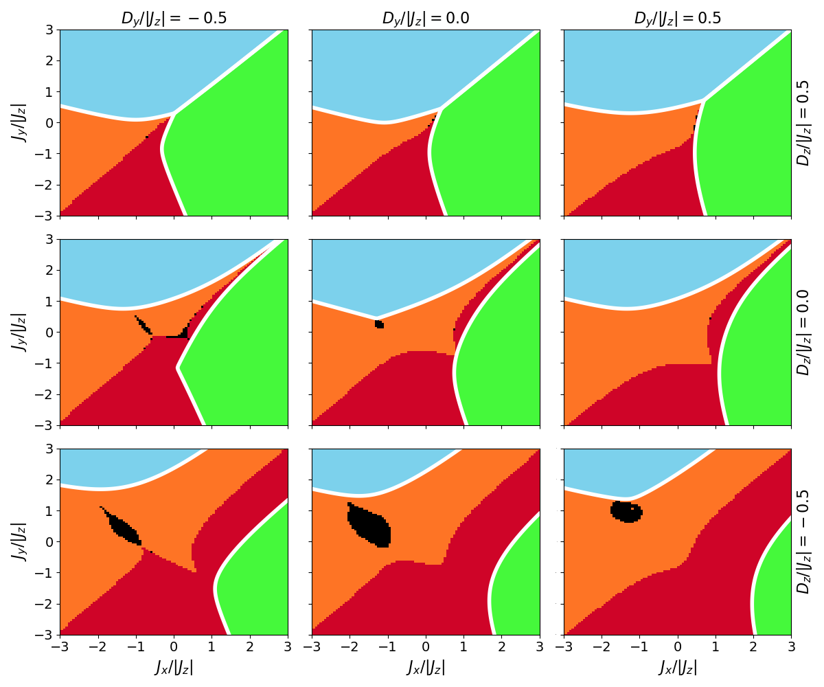
Figure 7: $T=0$ phase diagram with $J_{z}>0$ and $K=-0.5|J_{z}|$. Each panel shows a slice of the phase diagram as a function of $J_{x}$ and $J_{y}$ for different, fixed, values of the DM directions $D_{y}$ and $D_{z}$, with $D_{y}$ increasing from left to right and $D_{z}$ from bottom to top. The phase diagram is obtained by comparing numerically optimized energies for the five phases described in Section III. The numerical optimization procedure is described in Appendix A. The white lines show analytic calculations of the boundaries of the $\sf A_{1}$ and $\sf A_{2}$ phases, using conditions (27) and (28).

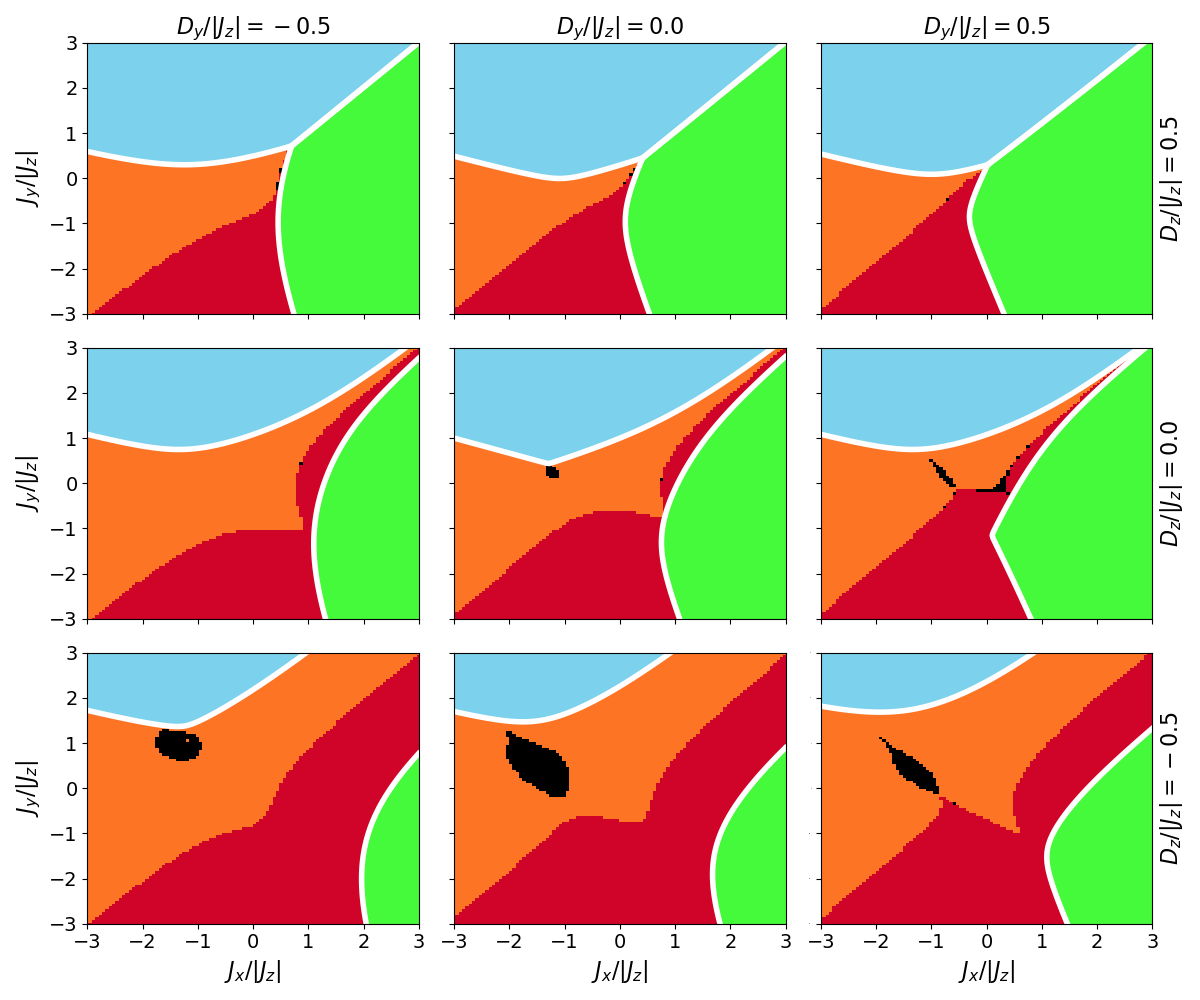
Figure 8: $T=0$ phase diagram with $J_{z}>0$ and $K=0.5|J_{z}|$. Each panel shows a slice of the phase diagram as a function of $J_{x}$ and $J_{y}$ for different, fixed, values of the DM directions $D_{y}$ and $D_{z}$, with $D_{y}$ increasing from left to right and $D_{z}$ from bottom to top. The phase diagram is obtained by comparing numerically optimized energies for the five phases described in Section III. The numerical optimization procedure is described in Appendix A. The white lines show analytic calculations of the boundaries of the $\sf A_{1}$ and $\sf A_{2}$ phases, using conditions (27) and (28).

IV Phase Diagram

In this section we calculate the ground state phase diagram of Eq. (1) numerically, by comparing optimized energies for the five phases described in Section III. The numerical optimization of the energy was done by a combination of random search, simulated annealing and iterative minimisation Sim and Lee (2018). Details of the numerics are given in Appendix A.

Figs. 7-10 show slices of the phase diagram as a function of $J_{x}/|J_{z}|$ and $J_{y}/|J_{z}|$ with $K/|J_{z}|=\{-0.5,0.5\}$ for both positive [Figs. 7- 8] and negative [Figs. 9- 10] $J_{z}$. Each panel in a given figure corresponds to different values of DM interactions $D_{y}/|J_{z}|$ and $D_{z}/|J_{z}|$. $D_{y}/|J_{z}|$ increases from left to right within each figure and $D_{z}/|J_{z}|$ from bottom to top. Taken together, Figs. 7-10 give a broad view of the competition between different magnetic orders as anisotropic exchange parameters are varied. Further phase diagrams, for a greater range and variety of parameter sets are shown in the Supplemental Material .

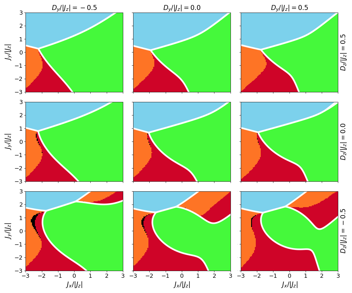
Figure 9: $T=0$ phase diagram with $J_{z}<0$ and $K=-0.5|J_{z}|$. Each panel shows a slice of the phase diagram as a function of $J_{x}$ and $J_{y}$ for different, fixed, values of the DM directions $D_{y}$ and $D_{z}$, with $D_{y}$ increasing from left to right and $D_{z}$ from bottom to top. The phase diagram is obtained by comparing numerically optimized energies for the five phases described in Section III. The numerical optimization procedure is described in Appendix A. The white lines show analytic calculations of the boundaries of the $\sf A_{1}$ and $\sf A_{2}$ phases, using conditions (27) and (28).

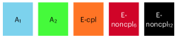
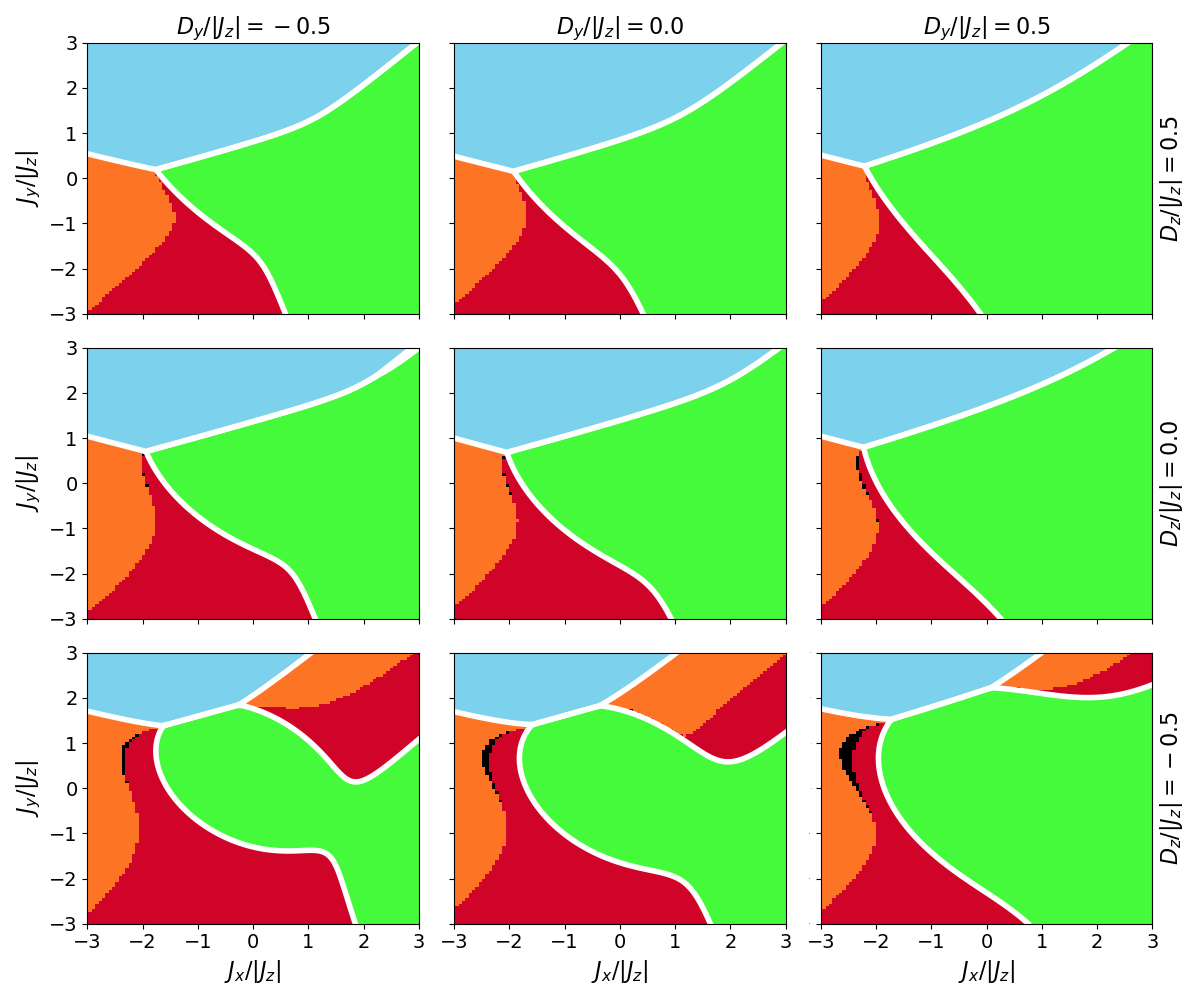
Figure 10: $T=0$ phase diagram with $J_{z}<0$ and $K=0.5|J_{z}|$. Each panel shows a slice of the phase diagram as a function of $J_{x}$ and $J_{y}$ for different, fixed, values of the DM directions $D_{y}$ and $D_{z}$, with $D_{y}$ increasing from left to right and $D_{z}$ from bottom to top. The phase diagram is obtained by comparing numerically optimized energies for the five phases described in Section III. The numerical optimization procedure is described in Appendix A. The white lines show analytic calculations of the boundaries of the $\sf A_{1}$ and $\sf A_{2}$ phases, using conditions (27) and (28).

The boundaries of the $A_{1}$ and $A_{2}$ phases can also be calculated analytically using conditions (27) and (28). These analytic boundaries are shown as white lines in Figs. 7-10, and agree with the results of the numerics. The boundaries between the different $\sf E$ phases are only calculated numerically.

One notable feature of Figs. 7-10 is that the ${\sf E}$-coplanar phase is generally found bordering the ${\sf A}_{1}$ phase, whereas the ${\sf E}$-noncoplanar₆ phase is generally found bordering the ${\sf A}_{2}$ phase. This is natural since the ${\sf E}$-coplanar phase mixes in a finite value of the ${\sf A}_{1}$ order parameter and likewise the ${\sf E}$-noncoplanar₆ includes a finite ${\sf A}_{2}$ order parameter.

Another striking feature of the phase diagram is the rarity of the ${\sf E}$-noncoplanar₁₂ phase. This low-symmetry configuration occupies only small portions of the phase diagrams in Figs. 7-10, with its stability generally being increased by a strong negative value of $D_{z}$.

To investigate the relative frequency of the different phases in the overall parameter space we have calculated the ground state for $100000$ different parameter sets, randomly chosen from a uniform distribution on the surface of the 6-dimensional hypersphere defined by

$$J_{x}^{2}+J_{y}^{2}+J_{z}^{2}+D_{y}^{2}+D_{z}^{2}+K^{2}=1.$$ (61)

The pie chart in Fig. 11(a) shows the relative frequency of each of the five phases obtained from this procedure. It confirms that ${\sf E}$-noncoplanar₁₂ is indeed a rare phase, found as the ground state for only $\sim 0.5\%$ of randomly generated parameter sets. The four other phases are comparatively common.

This leads us to conclude although the ${\sf E}$-noncoplanar₁₂ state does not require perfect fine tuning to be realized in a kagome material (i.e. it occupies a finite fraction of parameter space), it is unlikely to be realized serendipitously. The other four phases should constitute the classical ground states for the vast majority of kagome materials to which the theory in this paper can be applied (i.e. those with nearest-neighbour, anisotropic interactions).

The above assumes a probability distribution of parameter sets which is isotropic in the 6-dimensional space $(J_{x},J_{y},J_{z},D_{y},D_{z},K)$. This may not be the case physically, and indeed it is frequently assumed that the off-diagonal components of the exchange tensor $D_{y},D_{z},K$ should be smaller than the diagonal ones $J_{x},J_{y},J_{z}$. We have investigated the distribution of ground states under this assumption, by generating $100000$ random parameter sets by choosing $J_{x},J_{y},J_{z}$ from a uniform distribution on the surface of the unit sphere:

$$J_{x}^{2}+J_{y}^{2}+J_{z}^{2}=1$$ (62)

and indepently choosing $D_{y},D_{z},K$ from a uniform distribution on the surface of a smaller sphere:

$$D_{y}^{2}+D_{z}^{2}+K^{2}=0.1.$$ (63)

The resulting distribution of ground states is shown in Fig. 11(b). The relative frequency of different phases is very similar to that with an isotropic distribution of parameters, although the prevalence of the ${\sf E}$-noncoplanar₁₂ phase increases from $\sim 0.5/\%$ to $\sim 2/\%$.

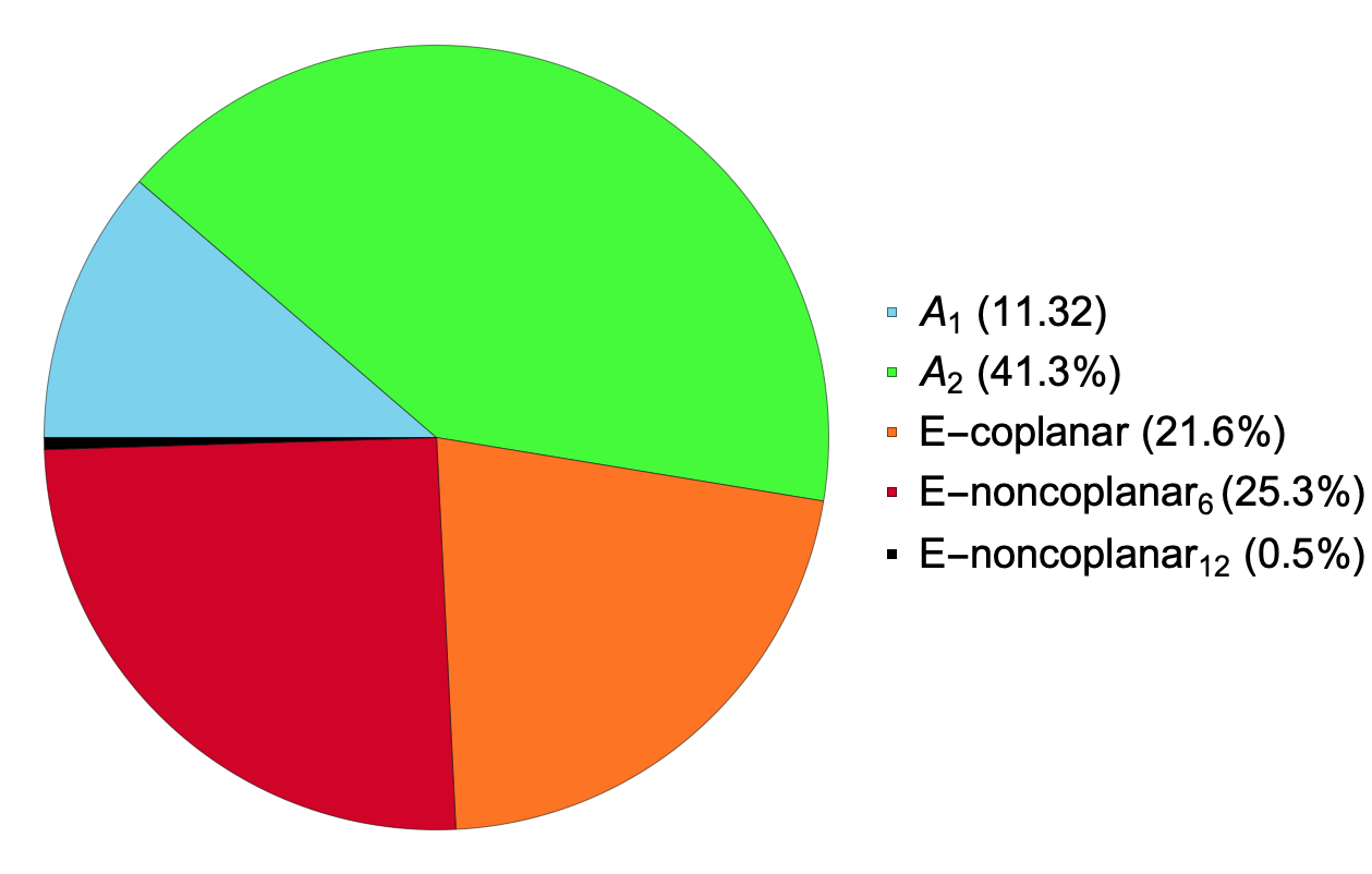
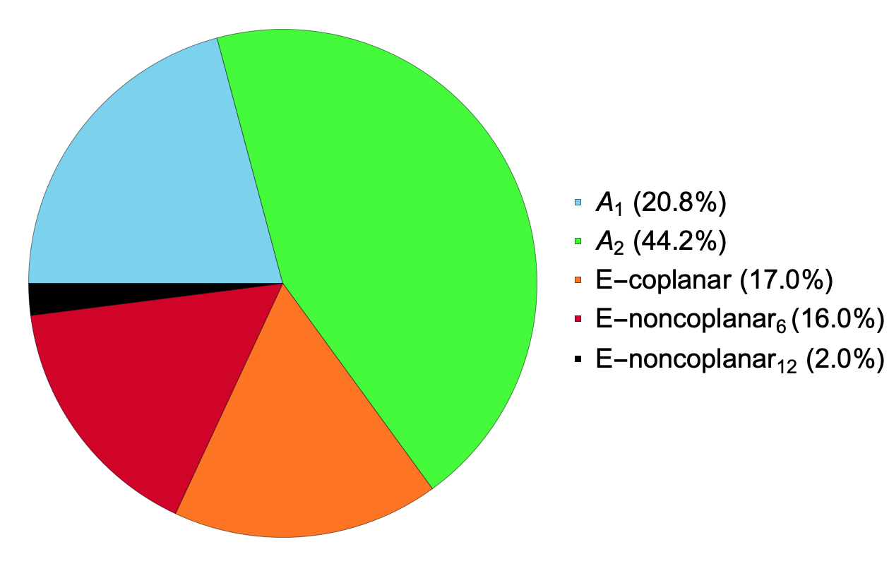
Figure 11: Relative frequency of different phases within the full parameter space of the Hamiltonian [Eq. (1)], with exchange parameters generated randomly from two different distributions. (a) Exchange parameters are generated randomly according to a uniform distribution on the surface of the 6-dimensional hypersphere defined by Eq. (61). (b) Diagonal exchange parameters $J_{x},J_{y},J_{z}$ are generated according to a uniform distribution on the surface of a sphere with unit radius, and off-diagonal $D_{y},D_{z},K$ exchange parameters are generated independently from a uniform distribution on the surface of a sphere with radius$=0.1$ [Eqs. (62)-(63)]. This models the effect of the assumption that the scale of off-diagonal couplings is lower. The effect on the distribution of phases is minor overall, although assuming weaker off-diagonal exchange expands the size of the rare ${\sf E}$-noncoplanar₁₂ from $\sim 0.5\%$ to $\sim 2\%$ In each case, frequencies are determined by numerically finding the ground state for 100000 random parameter sets generated according to the stated distributions.

IV.1 Phase diagram in the vicinity of the Antiferromagnetic Heisenberg limit

The limit $J_{x}=J_{y}=J_{z}=J>0$, $D_{y}=K=D_{z}=0$, gives the well studied nearest neighbor antiferromagnetic Heisenberg model, which is known to have a highly degenerate ground state Reimers et al. (1991). Generic perturbations away from this limit lift the degeneracy, stabilizing a ground state which is unique up to global symmetry operations.

Fig. 12 shows the effect of perturbing the Heisenberg model with finite off-diagonal couplings $D_{y},D_{z},K$. $D_{z}>0$ strongly favours $\sf A_{2}$ order, while $D_{z}<0$ favours ordering into the ${\sf E}$-coplanar or ${\sf E}$-noncoplanar₆ phases depending on which of $D_{y}$ or $K$ is the more dominant perturbation. Our results are in agreement with those of Elhajal et al Elhajal et al. (2002), who considered the case of perturbing the Heisenberg model with Dzyaloshinskii-Moriya interactions $D_{y},D_{z}$, fixing $K=0$.

When comparing the results here with those of [Elhajal et al., 2002] one should note that the ground state configurations of the ${\sf E}-{\rm noncoplanar}_{6}$ phase become coplanar in the limit of strong positive $J$ and $K=0$. This agrees with the labelling of the same phase as coplanar in [Elhajal et al., 2002]. Once all symmetry allowed couplings (particularly $K$) are present, this phase becomes non-coplanar, as identified here.

It is notable that the $\sf A_{1}$ phase does not appear at all in Fig. 12. This can be readily understood from the couplings in Eqs. (14-20). When $J_{x}=J_{y}$, $\lambda_{\sf A_{1}}=\lambda_{\sf A_{2},bb}$. This then implies that $\omega_{{\sf A_{2}}0}\leq\lambda_{\sf A_{1}}$ [cf. Eqs. (25), (27)] with the equality only applying when $\lambda_{\sf A_{2},ab}=2(\sqrt{3}D_{y}+K)=0$.

Thus, when $J_{x}=J_{y}$ the ${\sf A_{2}}$ phase will quite generally have a lower energy than the ${\sf A}_{1}$ phase. A necessary (but not sufficient) condition for the ${\sf A}_{1}$ configurations to be the sole ground states is that $\lambda_{\sf A_{1}}<\lambda_{\sf A_{2}bb}\implies J_{x}<J_{y}$.

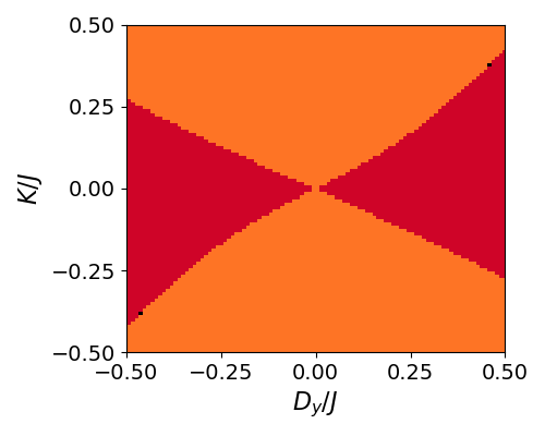
(a)  $D_{z}=-0.25J$

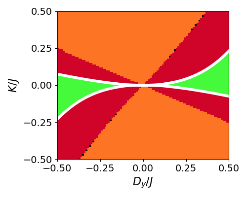
(b)  $D_{z}=0$

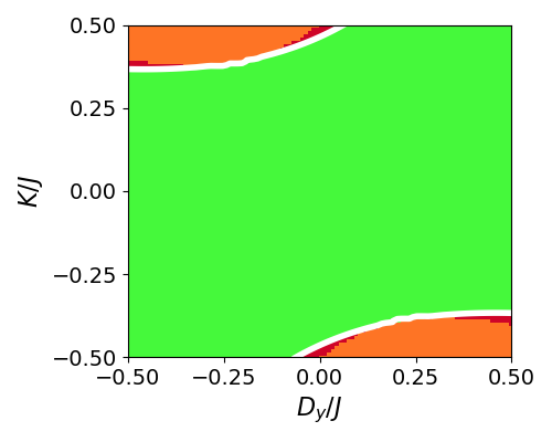
(c)  $D_{z}=0.25J$

Figure 12: Ground state phase diagram obtained from perturbing the antiferromagnetic Heisenberg model ($J_{x}=J_{y}=J_{z}=J>0$) with off-diagonal couplings $D_{y},D_{z},K$. Phase diagrams are shown as a function of $D_{y}/J,K/J$ at fixed values of $D_{z}/J=-0.25$ [(a)], $D_{z}/J=0$ [(b)], $D_{z}/J=0.25$ [(c)] The phase diagram is obtained by comparing numerically optimized energies for the five phases described in Section III. The numerical optimization procedure is described in Appendix A. The $\sf A_{1}$ phase does not appear on these phase diagrams, as it can only be stabilized as a unique ground state when $J_{x}<J_{y}$, whereas $J_{x}=J_{y}$ here. The white lines show analytic calculations of the boundaries of the $\sf A_{2}$ phase, using condition (28).

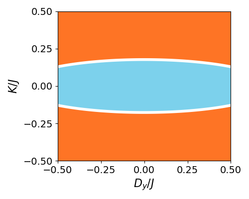
(a)  $\delta J_{\perp}=-0.25J$

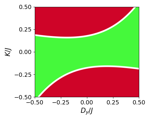
(b)  $\delta J_{\perp}=0.25J$

Figure 13: Ground state phase diagram obtained from perturbing the antiferromagnetic Heisenberg model with off-diagonal couplings $D_{y},K$, and anisotropy in the transverse exchange $J_{x}=J+\frac{\delta J_{\perp}}{2},J_{y}=J-\frac{\delta J_{\perp}}{2}$. We set $J_{z}=J>0$ and $D_{z}=0$ in both panels. Phase diagrams are shown as a function of $D_{y}/J,K/J$ at fixed values of $\delta J_{\perp}/J=-0.25$ [(a)], $\delta J_{\perp}/J=0.25$ [(b)] The phase diagram is obtained by comparing numerically optimized energies for the five phases described in Section III. The numerical optimization procedure is described in Appendix A. The white lines show analytic calculations of the boundaries of the $\sf A_{1}$ and $\sf A_{2}$ phases, using conditions (27)-(28).

The effect of allowing small anisotropy in the transverse exchanges $J_{x},J_{y}$ is illustrated in Fig. 13. Here we set

$$D_{z}=0,\ J_{z}=J>0,\ J_{x}=J+\frac{\delta J_{\perp}}{2},\ J_{y}=J-\frac{\delta J_{\perp}}{2}$$

and vary $D_{y}/J$ and $K/J$. As implied by the discussion above, $\delta J_{\perp}<0$ favours ${\sf A}_{1}$ order, becoming unstable to the ${\sf E}$-coplanar phase on increasing $K$. Conversely, when $\delta J_{\perp}>0$ favours ${\sf A}_{2}$ order, which gives way to the ${\sf E}$-noncoplanar₆ phase for strong $K$.

V Relevance to kagome materials

In this section we discuss the application of our results to real kagome materials. We divide our discussion into two areas: firstly, rare-earth magnets belonging to the family R₃A₂Sb₃O₁₄ Sanders et al. (2016a, b); Scheie et al. (2016); Dun et al. (2016); Scheie et al. (2016); Dun et al. (2017); Scheie et al. (2018); Ding et al. (2018); Scheie et al. (2019) (sometimes referred to as “tripod kagome” materials Dun et al. (2016, 2017)), and secondly, Cu, Fe and Cr based magnets where exchange anisotropy should be weaker but nevertheless plays a role in ground state selection.

Aside from the systems mentioned below, we anticipate that ongoing work in synthesizing frustrated magnets with strong spin-orbit coupling will reveal new kagome systems to which our results can be applied in the coming years.

V.1 $\text{R}_{3}\text{A}_{2}\text{Sb}_{3}\text{O}_{14}$ family

In the last few years several rare-earth kagome materials with the general formula $\text{R}_{3}\text{A}_{2}\text{Sb}_{3}\text{O}_{14}$ have been synthesized. This includes materials with A=Mg, Zn and R=Pr, Nd, Sm, Eu, Gd, Tb, Dy, Ho, Er, Tm, Yb Sanders et al. (2016a, b); Dun et al. (2017); Ding et al. (2018).

Where R is a non-Kramers ion (Pr, Eu, Tb, Ho, Tm), the crystal electric field (CEF) will generally have a non-magnetic singlet ground state, due to the low symmetry of the rare-earth environment. If the gap between this singlet and higher CEF states is smaller than or comparable to the energy scale of interactions, interesting physics may ensue. If the CEF gap is large, the overall ground state of the system will be a trivial singlet driven by the onsite physics. Either way, Eq. (1) cannot describe such physics without being augmented by additional terms, so we will not discuss non-Kramers materials further here.

Where $R$ is a Kramers ion, the CEF will split the 2J+1 multiplet into a series of doublets. At energy and temperature scales below the gap between the lowest and first excited doublet, the magnetism may be represented by pseudospin-$1/2$ operators ${\bf S}_{i}$. ${\bf S}_{i}$ does not correspond precisely to the magnetic moment, but relates to it via the $g$-tensor [Eq. 2]. The important thing for our purposes is that ${\bf S}_{i}$ transforms like a magnetic moment with respect to time-reversal and lattice symmetries, in which case Eqs. (1)-(6) describe the exchange interactions. Below we briefly discuss the various members of the $\text{R}_{3}\text{A}_{2}\text{Sb}_{3}\text{O}_{14}$ family, with Kramers ions $R$, in the light of the predictions made in this Article.

The scalar chiral order observed in Nd₃Mg₂Sb₃O₁₄ Scheie et al. (2016, 2019) corresponds precisely to the ${\sf A_{2}}$ phase predicted in this work. The magnetic order of the sister compound Nd₃Zn₂Sb₃O₁₄ has not yet been characterized, but given its essentially similar thermodynamic properties Dun et al. (2017) and crystal field environment Scheie et al. (2018) it seems likely to fall in the same phase as Nd₃Mg₂Sb₃O₁₄.

Er₃Mg₂Sb₃O₁₄ was reported in Ref. Dun et al., 2017 to avoid long range order down to very low temperatures. It thus appears to be a candidate spin liquid material. The regions near the phase boundaries of the classical phase diagram presented here are likely to be particularly fertile ground for the formation of spin liquid states, and this will be an interesting direction for future research. Er₃Zn₂Sb₃O₁₄ exhibits strong structural disorder and associated glassy behavior of the magnetic properties Dun et al. (2017), which is beyond the scope of our present discussion.

Yb₃Mg₂Sb₃O₁₄ exhibits long range order at $T_{N}\approx 0.88$K Dun et al. (2017). The form of this magnetic order has yet to be reported in the literature. Based on the expectation that, as a rare earth magnet with moderate magnetic moment, the theory in this manuscript should be applicable to Yb₃Mg₂Sb₃O₁₄, we expect that the order will be one of the states discussed in this work. Like Er₃Zn₂Sb₃O₁₄, Yb₃Zn₂Sb₃O₁₄ has strong structural disorder, although unlike the Er compound it does not show clear signs of spin freezing Dun et al. (2017).

Sm₃Mg₂Sb₃O₁₄ Sanders et al. (2016a) and Sm₃Zn₂Sb₃O₁₄ Sanders et al. (2016b) have both been synthesized but their low temperature magnetism has yet to be characterized in detail. This may be challenging due to the small magnetic moment of the Sm³⁺ ion, but recent experiments on the pyrochlores Sm₂Ti₂O₇ and Sm₂Sn₂O₇ indicate that this is possible Peçanha-Antonio et al. (2019). There is some evidence of hysteresis in the low temperature magnetization curve for Sm₃Zn₂Sb₃O₁₄ Sanders et al. (2016b) but not for Sm₃Mg₂Sb₃O₁₄ Sanders et al. (2016a), which may provide some clue as to the low temperature state.

Materials with R=Gd present a somewhat different case, because Hund’s rules imply vanishing orbital angular momentum $L=0$ for the Gd³⁺ ion. The magnetism on the Gd sites thus comes from a pure $S=7/2$ spin and anisotropies in the interactions should be much weaker. Some understanding of this case can be gained from considering a model with nearest neighbor Heisenberg exchange and the nearest-neighbor part of the dipolar interaction:

$$\mathcal{H}=J\sum_{\langle ij\rangle}{\bf S}_{i}\cdot{\bf S}_{j}+\tilde{D}_{\sf nn}\sum_{\langle ij\rangle}\left({\bf S}_{i}\cdot{\bf S}_{j}-3{\bf S}_{i}\cdot\hat{\bf r}_{ij}{\bf S}_{j}\cdot\hat{\bf r}_{ij}\right)$$

(64)

In terms of the symmetry-allowed interaction matrices [Eqs. (4)-(6)] this Hamiltonian corresponds to setting

$$J_{x}=J-2\tilde{D}_{\sf nn},\ J_{y}=J_{z}=J+\tilde{D}_{\sf nn},$$

$$D_{y}=D_{z}=K=0.$$ (65)

Inserting Eq. (65) into Eqs. (14)-(23) leads us to the conclusion that for $J,\tilde{D}_{\sf nn}>0$, the $A_{1}$ configuration is favored out of the forms of order considered in this Article. This agrees with the conclusions of Maksymenko et al Maksymenko et al. (2015), who studied the phase diagram incorporating isotropic nearest neighbor exchange $J$ with the full long ranged dipolar interaction $D$, and found the $A_{1}$ configuration as the ground state for weak to moderate $D$ and antiferromagnetic $J$. It also agrees with previous predictions about the ground state of Gd₃Mg₂Sb₃O₁₄ Dun et al. (2016), and with the observed antiferromagnetic transition at $T_{N}\approx 1.7K$ Dun et al. (2016); Wellm et al. (2020), although differences between the field cooled and zero-field cooled susceptibility Wellm et al. (2020) remain to be understood.

For R=Dy the ionic magnetic moment is very large and the long range component of the dipolar interaction cannot be ignored. Dy₃Mg₂Sb₃O₁₄ exhibits an unusual “fragmented” Brooks-Bartlett et al. (2014) phase where there is an ordering of emergent “charge” degrees of freedom while spins remain partially disordered Paddison et al. (2016). The long-range dipole-dipole interaction plays a crucial role in this phenomenon Möller and Moessner (2009); Chern et al. (2011) and thus it is beyond the scope of the theory presented in this Article.

V.2 Nearly isotropic systems

While the most obvious application of the results in this Article is found in systems where exchange anisotropy is strong, our results can also be applied to understand cases where isotropic Heisenberg exchange is weakly perturbed by short ranged anisotropic interactions.

This is the case in the Fe- and Cr- jarosites AM₃(OH)₆(SO₄)₂ where M= {Fe, Cr} and A={K, Rb, NH₄, Na}Grohol et al. (2003); Nishiyama et al. (2003); Morimoto et al. (2003); Matan et al. (2006); Yildirim and Harris (2006). These are found to order in the $A_{2}$ phase - the most prevalent of our phase diagram. This is generally understood to be a consequence of antiferromagnetic Heisenberg exchange perturbed by a weak $D_{y}$. This interpretation fully agrees with the results presented here: it can readily be checked that inserting

$$J_{x}=J_{y}=J_{z}=J>0$$

$$D_{z}=K=0,\ \ |D_{y}|<<J$$ (66)

into Eqs. (14)-(23) gives an outcome obeying condition (28) and hence a ground state in the ${\sf A_{2}}$ phase [cf. Fig. 12]. What this work adds to the discussion is a simple and systematic approach to finding the preferred ground state for general kinds of anisotropic nearest neighbor perturbation.

An example where weak anisotropic perturbations away from a Heisenberg model lead to something other than ${\sf A_{2}}$ order is given by Cd-kapellasite Okuma et al. (2017). The weak ferromagnetic moment confined within the kagome planes in that material is only consistent with the ${\sf E}$-coplanar phase, out of the phases in this Article.

VI Summary and Discussion

In this Article we have developed a theory of the magnetic orders induced by nearest-neighbor exchange anisotropy in kagome magnets. Our theory reveals that five distinct magnetic orders can be expected from such interactions, all retaining the translational symmetry of the lattice, but being distinguished from one another by their transformations under time-reversal and point group symmetries. The five phases are: ${\sf A}_{1}$ [Fig. 2], ${\sf A}_{2}$ [Fig. 3], ${\sf E}$-coplanar [Fig. 4], ${\sf E}$-noncoplanar₆ [Fig. 5], ${\sf E}$-noncoplanar₁₂ [Fig. 6]. They are labelled according to the irreducible representation of the point group $C_{3v}$ with which the primary order parameter transforms, their coplanar or noncoplanar nature and their degeneracy. Eqs. (27)-(28) give exact conditions for the ${\sf A_{1}}$ and ${\sf A_{2}}$ configurations to be classical ground states.

We have used numerical calculations to determine the full zero temperature phase diagram of the most general anisotropic nearest-neighbor exchange model, showing the extent of these five phases [Figs. 7-10]. One of the five phases (${\sf E}$-noncoplanar₁₂) is found to be exceedingly rare in the parameter space [Fig. 11].

We have discussed how this theory relates to various real kagome materials [Section V], with both strong and weak exchange anisotropy.

The dominance of noncollinear (${\sf A}_{1}$, ${\sf E}$-coplanar) and noncoplanar ($A_{2}$, ${\sf E}$-noncoplanar_6,12) states on the phase diagram suggests a high possibility of spin excitations with topological band structures in many kagome materials Owerre (2017); Seshadri and Sen (2018); Mook et al. (2019). It is likely that the five phases identified here from analysis of broken symmetries can be subdivided further by the topology of the excitation bands. Relatedly, the possibility of coupling to itinerant electrons is an interesting area for future research with a view to investigating topological transport phenomena.

The approach used in this work relies on the ability to decompose the Hamiltonian into a sum over blocks, such that the ground state is obtained by finding the ground state on each block and tiling it over the lattice. This would seem to limit the usefulness of the approach for systems with further neighbor interactions, since such a decomposition may either not be possible or may require such large blocks that the decomposition is no longer a useful simplification. Applying the method from this work to quantum systems will also not be possible in general - even for nearest neighbor interactions - because the Hamiltonians on neighboring blocks will usually not commute. There are, however, some specific, fine-tuned, cases where the exact ground state of a quantum system can be built up by such a block-by-block approach Changlani et al. (2018); Palle and Benton .

While we have restricted ourselves here to phases which are stable over finite regions of the classical phase diagram, a study of the phase boundaries may also be interesting. As has been studied elsewhere Essafi et al. (2017); Yan et al. (2017) phase boundaries between competing classical phases can host non-trivial enlarged manifolds of zero-energy states, which in some cases are associated with new forms of spin liquid Benton et al. (2016). In general, the greater the degree of degeneracy around the phase boundary, the more more favorable the situation becomes towards the formation of spin liquids. Different phase boundaries will have different amounts of additional degeneracy and so some will be more favorable for spin liquid formation than others. Boundaries where 3 (rather than just 2) phases meet may host particularly interesting physics as seen in (e.g.) [Benton et al., 2016]. An analysis of each possible phase boundary would be an interesting undertaking, which we leave open for future work.

Appendix A Numerical optimization of energies

Here we describe the numerical optimization used to obtain the phase diagrams in Figs. 7-10 and the estimates of the relative frequency of phases in Fig. 11.

For a given parameter set, the energy is optimized separately for each of the five phases described in Section III and then the optimized energies are compared to determine which is the lowest.

Due to the argument in Section III.1, we need only optimize the configuration on a single triangle, since we know that a ground state on the full lattice can be obtained by tiling the ground state of a single triangle everywhere.

The optimization for each phase is done by either random search or simulated annealing combined with iterative minimization Sim and Lee (2018), apart from the $A_{1}$ phase where the spin configuration is fixed [Eq. 33] and thus the corresponding energy can directly be calculated without any optimization being necessary:

$$E_{\sf A_{1}}=\frac{3}{4}\left(-2\sqrt{3}D_{z}+J_{x}-3J_{y}\right).$$ (67)

For the other four phases (${\sf A}_{2}$, ${\sf E}$-coplanar, ${\sf E}$-noncoplanar₆, ${\sf E}$-noncoplanar₁₂), the optimization procedure is as described below.

A.1 Optimizing ${\sf A_{2}}$ configuration

The form for the $\sf A_{2}$ configurations is given in Eq. (34). This can be written as

$${\bf S}_{0}=\left(-\frac{\sqrt{3}}{2}s_{a},s_{a}/2,s_{b}\right)$$ (68)

$${\bf S}_{1}=\left(\frac{\sqrt{3}}{2}s_{a},s_{a}/2,s_{b}\right)$$ (69)

$${\bf S}_{2}=\left(0,-s_{a},s_{b}\right)$$ (70)

with $(s_{a},s_{b})$ on the unit circle

$$s_{a}^{2}+s_{b}^{2}=1.$$ (71)

Initially, we calculate the energy for $10^{5}$ randomly generated values of $(s_{a},s_{b})$ on the unit circle. The lowest energy configuration obtained from this random search is then used as input for the iterative minimization step.

In the iterative minimization step $(s_{a},s_{b})$ are updated as

$$s_{a}\to\frac{s_{a}-c\frac{\partial E}{\partial s_{a}}}{|(s_{a}-c\frac{\partial E}{\partial s_{a}},s_{b}-c\frac{\partial E}{\partial s_{b}})|}$$

$$s_{b}\to\frac{s_{b}-c\frac{\partial E}{\partial s_{b}}}{|(s_{a}-c\frac{\partial E}{\partial s_{a}},s_{b}-c\frac{\partial E}{\partial s_{b}})|}.$$ (72)

For sufficiently small, positive, $c$ this update is guaranteed to reduce the energy, unless the system is already in a locally optimal configuration before the update.

The parameter $c$ is initially set to $0.1$. If the update (72) does not reduce the energy then $c$ is reduced by a factor of $2$ and the update is attempted again. This procedure is repeated until the configuration converges.

A.2 Optimizing ${\sf E}$-coplanar configuration

The form for an $\sf E$-coplanar configuration is given in Eq. (45). This can be rewritten as

$${\bf S}_{0}=\left(\sigma_{x},\sigma_{y},\sigma_{z}\right)$$ (73)

$${\bf S}_{1}=\left(\sigma_{x},-\sigma_{y},-\sigma_{z}\right)$$ (74)

$${\bf S}_{2}=\left(1,0,0\right)$$ (75)

with $(\sigma_{x},\sigma_{y},\sigma_{z})$ on the unit sphere

$$\sigma_{x}^{2}+\sigma_{y}^{2}+\sigma_{z}^{2}=1.$$ (76)

Initially, we calculate the energy for $10^{5}$ randomly generated values of $(\sigma_{x},\sigma_{y},\sigma_{z})$ on the unit sphere. The lowest energy configuration obtained from this random search is then used as input for the iterative minimization step.

In the iterative minimization step $(\sigma_{x},\sigma_{y},\sigma_{z})$ are updated as

$$\sigma_{\alpha}\to\frac{\sigma_{\alpha}-c\frac{\partial E}{\partial\sigma_{\alpha}}}{|(\sigma_{x}-c\frac{\partial E}{\partial\sigma_{x}},\sigma_{y}-c\frac{\partial E}{\partial\sigma_{y}},\sigma_{z}-c\frac{\partial E}{\partial\sigma_{z}})|}$$ (77)

The parameter $c$ is initially set to $0.1$. If the update (77) does not reduce the energy then $c$ is reduced by a factor of $2$ and the update is attempted again. This procedure is repeated until the configuration converges.

The set of configurations covered by the ${\sf E}$-coplanar ansatz (45) includes the ${A_{1}}$ configurations (when $\phi=\frac{4\pi}{3},\theta=\frac{\pi}{2}$). Because of this, if the ${\sf E}$-coplanar optimization is found to give the lowest energy of the five possibilities we must check that the obtained configuration has a nonzero value of at least one of the order parameters ${\bf m}_{{\sf E}\alpha}$. In practice we check that

$$|{\bf m}_{{\sf E}a}|^{2}+|{\bf m}_{{\sf E}b}|^{2}+|{\bf m}_{{\sf E}c}|^{2}>10^{-5}.$$ (78)

If the ${\sf E}$-coplanar optimization obtains the lowest energy but the inequality (78) is not fulfilled, the ground state is assigned to the ${\sf A}_{1}$ phase.

A.3 Optimizing ${\sf E}$-noncoplanar₆ configuration

The form for an $\sf E$-noncoplanar₆ configuration is given in Eq. (45). This can be rewritten as

$${\bf S}_{0}=\left(\tau_{x},\tau_{y},\tau_{z}\right)$$ (79)

$${\bf S}_{1}=\left(-\tau_{x},\tau_{y},\tau_{z}\right)$$ (80)

$${\bf S}_{2}=\left(0,t_{a},t_{b}\right)$$ (81)

with $(\tau_{x},\tau_{y},\tau_{z})$ on the unit sphere and $(t_{a},t_{b})$ on the unit circle

$$\tau_{x}^{2}+\tau_{y}^{2}+\tau_{z}^{2}=1$$ (82)

$$t_{a}^{2}+t_{b}^{2}=1.$$ (83)

Initially, we calculate the energy for $10^{5}$ randomly generated values of $(\tau_{x},\tau_{y},\tau_{z})$ and $(t_{a},t_{b})$ obeying Eqs. (82)-(83). The lowest energy configuration obtained from this random search is then used as input for the iterative minimization step.

In the iterative minimization step, we update the parameters according to the following:

$$\tau_{\alpha}\to\frac{\tau_{\alpha}-c\frac{\partial E}{\partial\tau_{\alpha}}}{|(\tau_{x}-c\frac{\partial E}{\partial\tau_{x}},\tau_{y}-c\frac{\partial E}{\partial\tau_{y}},\tau_{z}-c\frac{\partial E}{\partial\tau_{z}})|}$$

$$t_{\alpha}\to\frac{t_{\alpha}-c\frac{\partial E}{\partial t_{\alpha}}}{|(t_{a}-c\frac{\partial E}{\partial t_{a}},t_{b}-c\frac{\partial E}{\partial t_{b}})|}$$ (84)

The parameter $c$ is initially set to $0.1$. If the update (84) does not reduce the energy then $c$ is reduced by a factor of $2$ and the update is attempted again. This procedure is repeated until the configuration converges.

The set of configurations covered by the ${\sf E}$-noncoplanar₆ ansatz (51) includes the ${A_{2}}$ configurations (when $\mu=-(\kappa-\frac{\pi}{2}),\nu=-\frac{\pi}{6}$). Because of this, if the ${\sf E}$-noncoplanar₆ optimization is found to give the lowest energy of the five possibilities we must check that the obtained configuration has a nonzero value of at least one of the order parameters ${\bf m}_{{\sf E}\alpha}$. Numerically, we check the condition (78). If the ${\sf E}$-noncoplanar₆ optimization obtains the lowest energy but the inequality (78) is not fulfilled, the ground state is assigned to the ${\sf A}_{2}$ phase.

A.4 Optimizing ${\sf E}$-noncoplanar₁₂ configuration

Because the ${\sf E}$-noncoplanar₁₂ state allows for any configuration of three spins on a single triangle, the configuration space of states is larger and we use simulated annealing rather than a purely random search for the initial optimization, before the iterative minimization step.

In the simulated annealing the three spins on a triangle are initialized in a random configuration. Updates are attempted one spin at a time, being certainly accepted if they reduce the energy and accepted with probability $\exp(-\delta E/T)$ if they increase the energy by an amount $\delta E$. Initially, the “temperature”, $T=0.2$ in units where $|J_{z}|=1$ (for Figs. 7- 10] ) or where $J_{x}^{2}+J_{y}^{2}+J_{z}^{2}+D_{y}^{2}+D_{z}^{2}+K^{2}=1$ (for Fig. 11(a)) or where $J_{x}^{2}+J_{y}^{2}+J_{z}^{2}=1$ (for Fig. 11(b)). The triangle is swept $10^{5}$ times at a given temperature, and the temperature is then reduced by a factor of 0.9. This procedure is repeated 200 times. There are than $10^{5}$ sweeps of the triangle with $T=0$, i.e. only accepting energy reducing updates.

The whole annealing procedure is performed from the start 3 times for each parameter set with the final output being the lowest energy configuration obtained over all three sweeps.

To converge the configuration further, there is then an iterative minimisation step where each spin component is updated as:

$$S_{i}^{\alpha}\to\frac{S_{i}^{\alpha}-c\frac{\partial E}{\partial S_{i}^{\alpha}}}{|(S_{i}^{x}-c\frac{\partial E}{\partial S_{i}^{x}},S_{i}^{y}-c\frac{\partial E}{\partial S_{i}^{y}},S_{i}^{z}-c\frac{\partial E}{\partial S_{i}^{z}})|}$$ (85)

The parameter $c$ is initially set to $0.1$. If the update (85) does not reduce the energy then $c$ is reduced by a factor of $2$ and the update is attempted again. This procedure is repeated until the configuration converges.

If the energy produced from this procedure is lower than the energy produced from optimizing within the ${\sf A}_{1}$, ${\sf A}_{2}$, $E$-coplanar or $E$-noncoplanar₆ phases, then the ground state may be within the $E$-noncoplanar₁₂ phase. Because the configuration on the triangle is completely general, to confirm that the configuration has not converged to one of the other phases we check that the inequality (78) is satisfied, and also check that:

$$m_{\sf A_{1}}^{2}>10^{-5}$$ (86)

$$m_{\sf A_{2}a}^{2}+m_{\sf A_{2}b}^{2}>10^{-5}.$$ (87)

If inequalities (78), (86), (87) are not satisfied, the ground state is assigned to one of the other phases depending on the values of the various ${\bf m}_{\gamma}$ [Table 1].

References

- Ramirez (1994) A. P. Ramirez, “Strongly geometrically frustrated magnets,” Annual Review of Materials Science 24, 453–480 (1994).
- Harris et al. (1997) M. J. Harris, S. T. Bramwell, D. F. McMorrow, T. Zeiske, and K. W. Godfrey, “Geometrical Frustration in the Ferromagnetic Pyrochlore ,” Phys. Rev. Lett. 79, 2554–2557 (1997).
- Henley (1989) C. L. Henley, “Ordering due to disorder in a frustrated vector antiferromagnet,” Phys. Rev. Lett. 62, 2056–2059 (1989).
- Iqbal et al. (2019) Y. Iqbal, T. Müller, P. Ghosh, M. J. P. Gingras, H. O. Jeschke, S. Rachel, J. Reuther, and R. Thomale, “Quantum and Classical Phases of the Pyrochlore Heisenberg Model with Competing Interactions,” Phys. Rev. X 9, 011005 (2019).
- Kitaev (2006) A. Kitaev, “Anyons in an exactly solved model and beyond,” Annals of Physics 321, 2–111 (2006).
- Rousochatzakis and Perkins (2017) I. Rousochatzakis and N. B. Perkins, “Classical Spin Liquid Instability Driven By Off-Diagonal Exchange in Strong Spin-Orbit Magnets,” Phys. Rev. Lett. 118, 147204 (2017).
- Yan et al. (2017) H. Yan, O. Benton, L. D. C. Jaubert, and N. Shannon, “Theory of multiple-phase competition in pyrochlore magnets with anisotropic exchange with application to , and ,” Phys. Rev. B 95, 094422 (2017).
- Essafi et al. (2017) K. Essafi, O. Benton, and L. D. C. Jaubert, “Generic nearest-neighbor kagome model: XYZ and Dzyaloshinskii-Moriya couplings with comparison to the pyrochlore-lattice case,” Phys. Rev. B 96, 205126 (2017).
- Zhu et al. (2018) Z. Zhu, P. A. Maksimov, S. R. White, and A. L. Chernyshev, “Topography of spin liquids on a triangular lattice,” Phys. Rev. Lett. 120, 207203 (2018).
- Zorko et al. (2010) A. Zorko, F. Bert, P. Mendels, K. Marty, and P. Bordet, “Ground State of the Easy-Axis Rare-Earth Kagome Langasite ,” Phys. Rev. Lett. 104, 057202 (2010).
- Ghosh et al. (2014) S. Ghosh, S. Datta, H. Zhou, M. J. R. Hoch, C. R. Wiebe, P. Schlottmann, and S. Hill, “Spin-cluster excitations in the rare-earth kagome system ,” Phys. Rev. B 90, 224405 (2014).
- Sharma et al. (2016) A.Z. Sharma, H.J. Silverstein, A.M. Hallas, G.M. Luke, and C.R. Wiebe, “Structure and magnetic properties of new Be-substituted langasites A3Ga3Ge2BeO14 (A=Pr, Nd, and Sm),” Journal of Solid State Chemistry 233, 14 – 22 (2016).
- Sanders et al. (2016a) M. B. Sanders, K. M. Baroudi, J. W. Krizan, O. A. Mukadam, and R. J. Cava, “Synthesis, crystal structure and magnetic properties of novel 2D kagome materials RE3Sb3Mg2O14 (RE=La, Pr, Sm, Eu, Tb, Ho): Comparsion to RE3Sb3Zn2O14 family,” Phys. Status Solidi B 253, 2056–2065 (2016a).
- Sanders et al. (2016b) M. B. Sanders, J. W. Krizan, and R. J. Cava, “RE3Sb3Zn2O14 (RE = La, Pr, Nd, Sm, Eu, Gd): a new family of pyrochlore derivatives with rare earth ions on a 2D Kagome lattice,” J. Mater. Chem. C 4, 541–550 (2016b).
- Dun et al. (2016) Z. L. Dun, J. Trinh, K. Li, M. Lee, K. W. Chen, R. Baumbach, Y. F. Hu, Y. X. Wang, E. S. Choi, B. S. Shastry, A. P. Ramirez, and H. D. Zhou, “Magnetic Ground States of the Rare-Earth Tripod Kagome Lattice (),” Phys. Rev. Lett. 116, 157201 (2016).
- Scheie et al. (2016) A. Scheie, M. Sanders, J. Krizan, Y. Qiu, R. J. Cava, and C. Broholm, “Effective spin- scalar chiral order on kagome lattices in ,” Phys. Rev. B 93, 180407(R) (2016).
- Dun et al. (2017) Z. L. Dun, J. Trinh, M. Lee, E. S. Choi, K. Li, Y. F. Hu, Y. X. Wang, N. Blanc, A. P. Ramirez, and H. D. Zhou, “Structural and magnetic properties of two branches of the tripod-kagome-lattice family ( = Mg, Zn; = Pr, Nd, Gd, Tb, Dy, Ho, Er, Yb),” Phys. Rev. B 95, 104439 (2017).
- Scheie et al. (2018) A. Scheie, M. Sanders, J. Krizan, A. D. Christianson, V. O. Garlea, R. J. Cava, and C. Broholm, “Crystal field levels and magnetic anisotropy in the kagome compounds , , and ,” Phys. Rev. B 98, 134401 (2018).
- Ding et al. (2018) Z.-F. Ding, Y.-X. Yang, J. Zhang, C. Tan, Z.-H. Zhu, G. Chen, and L. Shu, “Possible gapless spin liquid in the rare-earth kagome lattice magnet ,” Phys. Rev. B 98, 174404 (2018).
- Scheie et al. (2019) A. Scheie, S. Dasgupta, M. Sanders, A. Sakai, Y. Matsumoto, T. R. Prisk, S. Nakatsuji, R. J. Cava, and C. Broholm, “Homogenous reduced moment in a gapful scalar chiral kagome antiferromagnet,” Phys. Rev. B 100, 024414 (2019).
- Elhajal et al. (2002) M. Elhajal, Benjamin Canals, and C. Lacroix, “Symmetry Breaking due to Dzyaloshinsky-Moriya Interactions in the Kagomé Lattice,” Phys. Rev. B 66, 014422 (2002).
- Ballou et al. (2003) R. Ballou, B. Canals, M. Elhajal, C. Lacroix, and A.S. Wills, “Models for ordering in the jarosites Kagomé systems,” Journal of Magnetism and Magnetic Materials 262, 465 – 471 (2003).
- Cépas et al. (2008) O. Cépas, C. M. Fong, P. W. Leung, and C. Lhuillier, “Quantum phase transition induced by Dzyaloshinskii-Moriya interactions in the kagome antiferromagnet,” Phys. Rev. B 78, 140405(R) (2008).
- Messio et al. (2010) L. Messio, O. Cépas, and C. Lhuillier, “Schwinger-boson approach to the kagome antiferromagnet with Dzyaloshinskii-Moriya interactions: Phase diagram and dynamical structure factors,” Phys. Rev. B 81, 064428 (2010).
- Chernyshev and Zhitomirsky (2014) A. L. Chernyshev and M. E. Zhitomirsky, “Quantum Selection of Order in an XXZ Antiferromagnet on a Kagome Lattice,” Phys. Rev. Lett. 113, 237202 (2014).
- Götze and Richter (2015) O. Götze and J. Richter, “Ground-state phase diagram of the xxz spin- kagome antiferromagnet: A coupled-cluster study,” Phys. Rev. B 91, 104402 (2015).
- Essafi et al. (2016) K. Essafi, O. Benton, and L. D. C. Jaubert, “A Kagome Map of Spin Liquids from XXZ to Dzyaloshinskii-Moriya Ferromagnet,” Nat. Commun. 7, 10297 (2016).
- Changlani et al. (2018) H. J. Changlani, D. Kochkov, K. Kumar, B. K. Clark, and E. Fradkin, “Macroscopically Degenerate Exactly Solvable Point in the Spin- Kagome Quantum Antiferromagnet,” Phys. Rev. Lett. 120, 117202 (2018).
- Morita et al. (2018) Katsuhiro Morita, Masanori Kishimoto, and Takami Tohyama, “Ground-state phase diagram of the kitaev-heisenberg model on a kagome lattice,” Phys. Rev. B 98, 134437 (2018).
- Yang et al. (2020) Yang Yang, Natalia B. Perkins, Fulya Koç, Chi-Huei Lin, and Ioannis Rousochatzakis, “Quantum-classical crossover in the spin- heisenberg-kitaev kagome magnet,” Phys. Rev. Research 2, 033217 (2020).
- Grohol et al. (2003) D. Grohol, D. G. Nocera, and D. Papoutsakis, “Magnetism of pure iron jarosites,” Phys. Rev. B 67, 064401 (2003).
- Nishiyama et al. (2003) M. Nishiyama, S. Maegawa, T. Inami, and Y. Oka, “Magnetic ordering and spin dynamics in potassium jarosite: A Heisenberg kagomé lattice antiferromagnet,” Phys. Rev. B 67, 224435 (2003).
- Morimoto et al. (2003) T. Morimoto, M. Nishiyama, S. Maegawa, and Y. Oka, “Magnetization of New Kagomé Lattice Antiferromagnets: Cr-Jarosites, ACr3(OH)6(SO4)2 [A = Na, K, Rb, NH4],” Journal of the Physical Society of Japan 72, 2085–2090 (2003).
- Matan et al. (2006) K. Matan, D. Grohol, D. G. Nocera, T. Yildirim, A. B. Harris, S. H. Lee, S. E. Nagler, and Y. S. Lee, “Spin Waves in the Frustrated Kagomé Lattice Antiferromagnet ,” Phys. Rev. Lett. 96, 247201 (2006).
- Yildirim and Harris (2006) T. Yildirim and A. B. Harris, “Magnetic structure and spin waves in the Kagomé jarosite compound ,” Phys. Rev. B 73, 214446 (2006).
- Okuma et al. (2017) R. Okuma, T. Yajima, D. Nishio-Hamane, T. Okubo, and Z. Hiroi, “Weak ferromagnetic order breaking the threefold rotational symmetry of the underlying kagome lattice in ,” Phys. Rev. B 95, 094427 (2017).
- Onoda and Tanaka (2011) Shigeki Onoda and Yoichi Tanaka, “Quantum fluctuations in the effective pseudospin- model for magnetic pyrochlore oxides,” Phys. Rev. B 83, 094411 (2011).
- Chen (2019) Gang Chen, “Intrinsic transverse field in frustrated quantum ising magnets: Physical origin and quantum effects,” Phys. Rev. Research 1, 033141 (2019).
- Reimers et al. (1991) J. N. Reimers, A. J. Berlinsky, and A.-C. Shi, “Mean-field approach to magnetic ordering in highly frustrated pyrochlores,” Phys. Rev. B 43, 865–878 (1991).
- Sim and Lee (2018) G.-B. Sim and S.-B. Lee, “Discovery of a new type of magnetic order on pyrochlore spinels,” Phys. Rev. B 98, 014423 (2018).
- Note (1) See the Supplemental Material for a series phase diagrams as a function of and , with values of varying over , for both signs of .
- Peçanha-Antonio et al. (2019) V. Peçanha-Antonio, E. Feng, X. Sun, D. Adroja, H. C. Walker, A. S. Gibbs, F. Orlandi, Y. Su, and T. Brückel, “Intermultiplet transitions and magnetic long-range order in Sm-based pyrochlores,” Phys. Rev. B 99, 134415 (2019).
- Maksymenko et al. (2015) M. Maksymenko, V. R. Chandra, and R. Moessner, “Classical dipoles on the kagome lattice,” Phys. Rev. B 91, 184407 (2015).
- Wellm et al. (2020) C. Wellm, J. Zeisner, A. Alfonsov, M.-I. Sturza, G. Bastien, S. Gaß, S. Wurmehl, A. U. B. Wolter, B. Büchner, and V. Kataev, “Magnetic interactions in the tripod kagome antiferromagnet probed by static magnetometry and high-field esr spectroscopy,” Phys. Rev. B 102, 214414 (2020).
- Brooks-Bartlett et al. (2014) M. E. Brooks-Bartlett, S. T. Banks, L. D. C. Jaubert, A. Harman-Clarke, and P. C. W. Holdsworth, “Magnetic-moment fragmentation and monopole crystallization,” Phys. Rev. X 4, 011007 (2014).
- Paddison et al. (2016) J. A. M. Paddison, H. S. Ong, J. O. Hamp, P. Mukherjee, X. Bai, M. G. Tucker, N. P. Butch, C. Castelnovo, M. Mourigal, and S. E. Dutton, “Emergent Order in the Kagome Ising Magnet Dy3Mg2Sb3O14,” Nat. Commun. 7, 13842 (2016).
- Möller and Moessner (2009) G. Möller and R. Moessner, “Magnetic multipole analysis of kagome and artificial spin-ice dipolar arrays,” Phys. Rev. B 80, 140409(R) (2009).
- Chern et al. (2011) G.-W. Chern, P. Mellado, and O. Tchernyshyov, “Two-stage ordering of spins in dipolar spin ice on the kagome lattice,” Phys. Rev. Lett. 106, 207202 (2011).
- Owerre (2017) S. A. Owerre, “Topological thermal hall effect in frustrated kagome antiferromagnets,” Phys. Rev. B 95, 014422 (2017).
- Seshadri and Sen (2018) R. Seshadri and D. Sen, “Topological magnons in a kagome-lattice spin system with and Dzyaloshinskii-Moriya interactions,” Phys. Rev. B 97, 134411 (2018).
- Mook et al. (2019) A. Mook, J. Henk, and I. Mertig, “Thermal Hall effect in noncollinear coplanar insulating antiferromagnets,” Phys. Rev. B 99, 014427 (2019).
- (52) G. Palle and O. Benton, “Exactly solvable spin-1/2 xyz models with highly-degenerate, partially ordered, ground states,” arXiv:2101.12140 .
- Benton et al. (2016) O. Benton, L. D. C. Jaubert, H. Yan, and N. Shannon, “A spin-liquid with pinch-line singularities on the pyrochlore lattice,” Nat. Commun. 7, 11572 (2016).