Optimizing Program Size Using Multi-result Supercompilation

Abstract

Supercompilation is a powerful program transformation technique with numerous interesting applications. Existing methods of supercompilation, however, are often very unpredictable with respect to the size of the resulting programs. We consider an approach for controlling result size, based on a combination of multi-result supercompilation and a specific generalization strategy, which avoids code duplication. The current early experiments with this method show promising results – we can keep the size of the result small, while still performing powerful optimizations.

1 Introduction

Supercompilation was invented by Turchin [18] and has found numerous applications, such as program optimization[16, 17, 7], program analysis, software testing, formal verification [8, 14, 15]. It is closely related to partial evaluation [5] and deforestation. Different extensions of the basic supercompilation approach are also studied, aiming to further increase its power – for example, distillation [4], higher-level supercompilation [10], etc.

Supercompilation performs very powerful program transformations by simulating the actual execution of the input program on a whole set of possible inputs simultaneously. The flip side of this power is that the behavior of supercompilation – with respect to both transformation time and result size – can be very unpredictable. This makes supercompilation problematic for including as an optimization step of a standard compiler, for example. Measures have been proposed to make supercompilation more well-behaved, both in execution time and result size [2, 6], while still achieving substantial improvements in program run time. These proposals are all based on a combination of specially crafted and empirically fine-tuned heuristics. The main goal of the present study is to experiment with a more principled approach for finding a better balance between the size and the run-time performance of programs produced by supercompilation. This approach is based on a few key ideas:

• use multi-result supercompilation [9, 11, 3] to systematically explore a large set of different generalizations during the transformation process, leading to different trade-offs between performed optimizations and code explosion;

• carefully select a generalization scheme, which can – if applied systematically – avoid duplicating code during the supercompilation process itself;

• re-use ideas from Grechanik et al. [3] to compactly represent and efficiently explore the set of programs resulting from multi-result supercompilation.

We outline the main ideas of multi-result supercompilation – as well as the specific approach to its implementation that we use – in Sec. 2. We then describe the main contributions of this study:

• We propose a method of adapting some existing techniques (MRSC with efficient queries over result sets) to solve in a systematic way the problem of code explosion during supercompilation (Sec. 3).

• We define a particular strategy for generalization during MRSC (Sec. 3.3), which:

  • avoids any risk of duplicating code during supercompilation (when applied);

  • avoids unnecessary increase of the search space of possible transformed programs, which MRSC must explore.

• We analyze the performance of the proposed strategy on several simple examples (Sec. 4).

2 Summary of Multi-result Supercompilation

Supercompilation is often defined as a transformation of “configurations” – data structures containing information about the set of states of program execution currently being explored. The configurations are typically produced by a process called “driving”, and organized in “configuration trees”. Sometimes the current configuration is similar enough to some previous one, and we can “fold” the former to the latter, turning the configuration tree into a “configuration graph”. Finally, we can generate a new “residual” program from the configuration graph, where folding typically corresponds to calls to functions introduced by new recursive definitions. To ensure termination of the supercompilation process, a check – usually called a “whistle” – is systematically performed on the sequence of configurations being produced. When this whistle signals a potential risk of non-termination, one possibility to continue the supercompilation process is to perform a “generalization” – replace the current configuration by another, which avoids the non-termination risk, possibly by forgetting some information. The whistle usually marks the current configuration (“lower” in the tree) as risking non-termination with respect to some other configuration produced earlier (“higher” in the tree). Typical positive supercompilers – as described, for example, by Sørensen et al. [17] – make a choice whether to generalize the “lower” or the “upper” configuration. One of the key insights behind multi-result supercompilation is that the place where the whistle has blown is not always the best place to make a generalization. The proposed solution is radical: do not generalize when the whistle has blown; instead, at any driving step check if suitable generalizations exist and continue driving not only the non-generalized configuration, but also all generalized ones, giving rise to multiple alternative results of driving. This process is illustrated by the example at the end of Sec. 3.3.

Our implementation of multi-result supercompilation mostly follows the same generic framework used in [3, 13]. It offers some important simplifications compared to the original work of Klyuchnikov et al. [9, 11]:

• It is based on “big-step” driving (called so by analogy with big-step operational semantics, as driving a configuration produces the full configuration subtree corresponding to it).

• The whole set of transformed programs is represented compactly in a tree-like data structure, which further permits not only recovering the full set of configuration graphs, but also performing efficiently certain kinds of queries on this set.

The compact representation of the set of graphs is shown in Fig. 1. We use direct excerpts of the F# code of the implementation, but hopefully they will be readable by anyone familiar with other functional languages such as OCaml or Haskell. Another important caveat is that we have implemented MRSC for programs in a specific language, so some details will only become clear once we introduce this language. In particular, the configurations (MConf) we use are pairs of a multi-result driving step output and an expression of the language, as described in Sec. 3.3. A language-specific helper function buildGraph builds a configuration graph from a given configuration and subgraphs. Still, the details of the language are not important for understanding the core MRSC algorithm; indeed, such details are successfully abstracted away in [3, 13]. We prefer to show excerpts from our actual implementation for concreteness. The representation from Fig. 1 is termed lazy graph by Grechanik et al. [3], and can be viewed as a domain-specific language (DSL) describing the construction of the complete set of configuration graphs produced by multi-result supercompilation.

• Node GSNone is used when the whistle has blown. It represents an empty set of configuration graphs.

• Node GSFold is used when folding is possible. It gives the relative distance to the upper node to which we fold, plus the renaming (finite mapping of variables to variables), which makes the folded configurations compatible. Note that, following Grechanik et al. [3], we consider only folding to a node on the path from the current node to the root of the graph. This choice enables us to keep the representation of the set of configuration graphs we produce simpler. Also, similar to other positive supercompilers [16, 17, 7], it is only possible to fold to a node, which is a renaming of the current one.

• Node GSBuild is the most complicated one, representing a list of alternative developments (driving or generalization) of the current configuration. Each alternative, in turn, gives rise to a list of new configurations to explore, and hence, to a list of nested graph sets.

⬇

type MConf = MultiDriveStepResult * Exp

type GraphSet =

| GSNone

| GSFold of MConf * int * list<VarName * VarName>

| GSBuild of MConf * list<list<GraphSet>>

let rec gset2graphs (gs: GraphSet) : seq<MConf * ConfGraph> =

match gs with

| GSNone -> Seq.empty

| GSFold(conf, n, ren) -> Seq.singleton (conf, CGFold(n, ren))

| GSBuild(conf, alts) ->

let buildGraph’ subGraphs = (conf, buildGraph (snd conf) subGraphs)

let buildAlt alt =

Seq.map buildGraph’ (Seq.cartesian (Seq.map gset2graphs alt))

Seq.collect buildAlt alts

Figure 1: Representation and Expansion of Graph Sets

The semantics of this DSL is shown in the same Fig. 1 as a function gset2graphs expanding a GraphSet into a sequence of configuration graphs. Note the use of Seq.cartesian to compose the subgraphs of the graph node of each alternative configuration.

Algorithm 1 Main MRSC Algorithm

1:function mrScpRec($P,l,h,c$) $\triangleright$ $P$ – program (function definitions); $l$ – nesting level;

2:     $\triangleright$ $h$ – history (list of tuples: local/global flag; level; configuration); $c$ – configuration

3:     if $\exists(\_,l^{\prime},c^{\prime})\in h,\rho\textrm{ -- renaming}:c=\textit{rename}(c^{\prime},\rho)$ then

4:         return $\mathtt{GSFold}(c,l-l^{\prime},\rho)$

5:     else

6:         $\mathit{rs}\leftarrow\mathtt{multiDriveSteps}(P,c)$

7:         if $\exists(\mathtt{MDSRCases}\_)\in\mathit{rs}$ then

8:              $\mathit{hk}\leftarrow\mathtt{HEGlobal}$

9:              $\mathit{relHist}\leftarrow[(\mathit{hk}^{\prime},l,c)|\mathit{hk}^{\prime}=\mathtt{HEGlobal}]$

10:         else

11:              $\mathit{hk}\leftarrow\mathtt{HELocal}$

12:              $\mathit{relHist}\leftarrow\mathit{takeWhile}(\lambda(\mathit{hk}^{\prime},l,c).\mathit{hk}^{\prime}=\mathtt{HELocal},h)$

13:         end if

14:         if $\exists(\_,\_,c^{\prime})\in\mathit{relHist}:c^{\prime}\trianglelefteq c$ then $\triangleright$ $\trianglelefteq$ denotes homeomorphic embedding

15:              return $\mathtt{GSNone}$

16:         else

17:              $\mathit{css}\leftarrow\mathit{map}(\mathtt{mdsrSubExps},\mathit{rs})$

18:              $h^{\prime}\leftarrow(\mathit{hk},l,c)::h$

19:              return $\mathtt{GSBuild}(c,\mathit{map}(\lambda\mathit{cs}.\mathit{map}(\lambda c.\textsc{mrScpRec}(P,l+1,h^{\prime},c),\mathit{cs}),css))$

20:         end if

21:     end if

22:end function

23:function mrScp($P,c$)

24:     return $\textsc{mrScpRec}(P,0,[],c)$

25:end function

The main MRSC algorithm – the one that builds the graph set of a given initial configuration – is presented with some simplifications as Algorithm 1. We can ignore the details about splitting the configuration history into a local and a global one – they mostly follow established heuristics as in Sørensen et al. [16, 17]. The overall approach is simple - if folding is possible, we produce a fold node and stop pursuing the current configuration. Otherwise we check the whistle – in our case, the same homeomorphic embedding relation, which is used in other positive supercompilers [17]. If it blows, we stop immediately with an empty set of resulting graphs. When there is neither folding nor a whistle, we continue analyzing the execution of the current configuration – based on 2 language-specific functions:

• multiDriveSteps returns a number of alternatives for the current configuration – either a set of new configurations produced by a single step of driving, or by (possibly several different forms of) generalization.

• mdsrSubExps returns – for a given alternative produced by the previous function – the list of sub-configurations (in our case – subexpressions) that must be subjected to further analysis.

The implementation of both functions is described in Sec. 3. Once we have this list of lists of sub-configurations, we simply apply the same algorithm recursively, but with extended history. Readers familiar with the implementation details of other supercompilers are invited to compare them to the simplicity of this MRSC approach.

3 Generalization Approach

3.1 Programming Language

The object language we consider is a first-order functional language with ordinary (not pattern-matching) and pattern-matching function definitions. Its syntax is summarized in Fig. 2. A very similar language – with call-by-name semantics – is often used in many introductions to positive supercompilation [16, 17, 7]. A notable restriction in our case is that we omit if-expressions and a built-in generic equality. We use the convention that data constructors always start with an uppercase letter, while function and variable names start with a lowercase one. The patterns of any function definition must be exhaustive, not nested, and non-overlapping. As a technical detail, we do not make a distinction between ordinary and pattern-matching functions at each call site, as this information is uniquely determined by the function definition itself.

Expressions $e$ ::= $x$ variable $|$ $a(e_{\_}1,\ldots,e_{\_}n)$ call

Figure 2: Object Language Syntax

3.2 Driving

Let us recall what driving looks like for this simple language, in the case of positive supercompilation (which is a simplification of the more general approach pioneered by Turchin [18]). As a technical device, we define a single step of driving, producing a result of type DriveStepResult, as defined in Fig. 3

⬇

type DriveStepResult =

| DSRNone

| DSRCon of ConName * list<Exp>

| DSRUnfold of Exp

| DSRCases of VarName * list<Pattern * Exp>

Figure 3: Result of a Single Step of Driving

• We cannot drive a variable any further: $\mathtt{drive}\llbracket x\rrbracket=\mathtt{DSRNone}$;

• Driving a constructor results in a constructor node with all arguments available for further driving: $\mathtt{drive}\llbracket C(e_{\_}1,\ldots,e_{\_}n)\rrbracket=\mathtt{DSRCon}(C,e_{\_}1,\ldots,e_{\_}n)$;

• If we stumble upon a call to an ordinary function, we simply unfold its definition:
  $\mathtt{drive}\llbracket f(e_{\_}1,\ldots,e_{\_}n)\rrbracket$ $=$ $\mathtt{DSRUnfold}(e[x_{\_}1\rightarrow e_{\_}1,\ldots,x_{\_}n\rightarrow e_{\_}n])$, where $f(x_{\_}1,$ …$,x_{\_}n)=e\in P$ and $e[x_{\_}1\rightarrow e_{\_}1,\ldots,x_{\_}n\rightarrow e_{\_}n]$ denotes simultaneous substitution;

• The most interesting cases concern a call to a pattern-matching function, as the situation is different depending on the kind of the first argument:

  • $\mathtt{drive}\llbracket g(C(e^{\prime}_{\_}1,\ldots,e^{\prime}_{\_}m),e_{\_}1,\ldots,e_{\_}n)\rrbracket=$ $\mathtt{DSRUnfold}(e[x_{\_}1\rightarrow e^{\prime}_{\_}1,\ldots,x_{\_}m\rightarrow e^{\prime}_{\_}m,y_{\_}1\rightarrow e_{\_}1,\ldots,y_{\_}n\rightarrow e_{\_}n])$ where $g(C(x_{\_}1,\ldots,x_{\_}m),y_{\_}1,\ldots,y_{\_}n)=e\in P$;

  • $\mathtt{drive}\llbracket g(x,e_{\_}1,\ldots,e_{\_}n)\rrbracket$ $=$ $\mathtt{DSRCases}$ $(x,$ $\mathtt{propagate}$ $(x,p_{\_}1,(e_{\_}1,$ …$,e_{\_}n),e^{\prime}_{\_}1),$ …, $\mathtt{propagate}$ $(x,p_{\_}m,(e_{\_}1,$ …$,e_{\_}n),e^{\prime}_{\_}m))$ where $g(p_{\_}1,y_{\_}1,$ …$,y_{\_}n)=e^{\prime}_{\_}1,$ …$,g(p_{\_}m,y_{\_}1,$ …$,y_{\_}n)=e^{\prime}_{\_}m\in P$ and $\mathtt{propagate}$ performs positive information propagation by substituting (a suitable renaming of) $p_{\_}i$ for $x$ in the corresponding branch $i$;

  • $\mathtt{drive}$ $\llbracket g(f(e^{\prime}_{\_}1,$ …$,e^{\prime}_{\_}m),$ $e_{\_}1,$ …$,e_{\_}n)\rrbracket$ $=$ $\mathtt{dsrMap}$$(\llbracket g(\bullet,e_{\_}1,$ …$,e_{\_}n)\rrbracket,$ $\mathtt{drive}\llbracket f(e^{\prime}_{\_}1,$ …$,e^{\prime}_{\_}m)\rrbracket)$ where $\mathtt{dsrMap}$ transforms a driving step result by splicing it in an expression with a hole.

We deliberately omit many low-level details in this description, as they are well-known and can be found in most introductions to positive supercompilation [16, 17, 7]. Using this definition of driving, plus the usual definitions of folding, whistle, and generalization, we can build configuration graphs of the form shown in Fig. 4. Note that we use the same representation of variables inside object-language programs and inside configuration graphs, as no confusions arise (assuming suitable measures for avoiding variable capture).

⬇

type ConfGraph =

| CGLeaf of Exp

| CGCon of ConName * list<ConfGraph>

| CGUnfold of ConfGraph

| CGCases of VarName * list<Pattern * ConfGraph>

| CGFold of int * list<VarName * VarName>

| CGLet of list<VarName * ConfGraph> * ConfGraph

Figure 4: Representation of a Configuration Graph

3.3 Multi-result Driving And Generalization

As already mentioned, a key difference in multi-result supercompilation is that driving and generalization are grouped together: a multi-driving step can return not one, but several alternative configurations. One of them is typically the result of standard driving, but the others can be different kinds of generalizations. The choice of generalization strategy depends on the intended use of the multi-result supercompiler. In our case, the main goal is to find a program of optimal size among the results. Previous analyses have shown that one of the main reasons for code size explosion in supercompilation is the unrestricted duplication of subexpressions during driving. Of course, sometimes such duplication pays off, as it leads to new opportunities for optimization. But this is not always the case. These observations lead us to consider two guiding principles that should help us attain our goal:

• if standard driving can duplicate existing code, provide also a generalized configuration, where no existing (non-trivial) subexpressions are duplicated;

• if there is no risk of duplicating code, avoid any generalization, as it will be unlikely to help with the size of the result.

To apply these principles, we analyze standard driving, case by case, to see where we need to avoid code duplication by generalization. In order to express generalization as a possible result of a driving step, we extend our representation of a step result - Fig. 5. The same figure shows the implementation of mdsrSubExps that we have encountered earlier. The source function multiDriveSteps will be denoted $\mathtt{mrdrive}$ for brevity below.

⬇

type MultiDriveStepResult =

| MDSRLeaf of Exp

| MDSRCon of ConName * list<Exp>

| MDSRUnfold of Exp

| MDSRCases of VarName * list<Pattern * Exp>

| MDSRLet of list<VarName * Exp> * Exp

let mdsrSubExps (mdsr: MultiDriveStepResult) : list<Exp> =

match mdsr with

| MDSRLeaf _ -> []

| MDSRCon(_, es) -> es

| MDSRUnfold e -> [e]

| MDSRCases(_, cases) -> List.map snd cases

| MDSRLet(binds, e) -> e :: List.map snd binds

Figure 5: One Step of Multi-result Driving

• The variable case is again trivial:
  $\mathtt{mrdrive}\llbracket x\rrbracket=[\mathtt{MDSRLeaf}(x)]$; (We use $[\ldots;\ldots;\ldots]$ to denote a list of results.)

• Driving a constructor does not duplicate code, so we again make no generalization:
  $\mathtt{mrdrive}\llbracket C(e_{\_}1,\ldots,e_{\_}n)\rrbracket=[\mathtt{MDSRCon}(C,e_{\_}1,\ldots,e_{\_}n)]$;

• The unfolding of a call to an ordinary function can produce code duplication, if some arguments appear multiple times in the body of the definition. We conservatively generalize all arguments of the call:
  $\mathtt{mrdrive}\llbracket f(e_{\_}1,\ldots,e_{\_}n)\rrbracket=$ $[\mathtt{MDSRLet}(y_{\_}1=e_{\_}1,$ …$,y_{\_}n=e_{\_}n,e[x_{\_}1\rightarrow y_{\_}1,$ …$,x_{\_}n\rightarrow y_{\_}n]);$ $\mathtt{MDSRUnfold}($ $e[x_{\_}1\rightarrow e_{\_}1,$ …$,x_{\_}n\rightarrow e_{\_}n])]$, where $y_{\_}1,\ldots,y_{\_}n$ are fresh and $f(x_{\_}1,\ldots,x_{\_}n)=e\in P$. Notice that we shall always place the generalization result before the driving result in the list. In this way, when we expand the lazy graph using gset2graphs, configuration graphs earlier in the resulting sequence will have more generalizations;

• The case of a pattern-matching call with a known constructor is completely analogous to the previous one:
  $\mathtt{mrdrive}\llbracket g(C(e^{\prime}_{\_}1,$ …$,e^{\prime}_{\_}m),e_{\_}1,$ …$,e_{\_}n)\rrbracket=[$ $\mathtt{MDSRLet}(u_{\_}1=e^{\prime}_{\_}1,$ …$,u_{\_}m=e^{\prime}_{\_}m,z_{\_}1=e_{\_}1,$ …$,z_{\_}n=e_{\_}n,$ $e[x_{\_}1\rightarrow u_{\_}1,$ …$,x_{\_}m\rightarrow u_{\_}m,y_{\_}1\rightarrow z_{\_}1,$ …$,y_{\_}n\rightarrow z_{\_}n]);$ $\mathtt{MDSRUnfold}(e[x_{\_}1\rightarrow e^{\prime}_{\_}1,$ …$,x_{\_}m\rightarrow e^{\prime}_{\_}m,y_{\_}1\rightarrow e_{\_}1,$ …$,y_{\_}n\rightarrow e_{\_}n])]$ where $u_{\_}1,\ldots,u_{\_}m,z_{\_}1,\ldots,z_{\_}n$ are fresh and $g(C(x_{\_}1,\ldots,x_{\_}m),y_{\_}1,\ldots,y_{\_}n)=e\in P$;

• When we pattern-match on a variable, information propagation can introduce some code duplication. The code potentially being duplicated, however, is always of the form $C(x_{\_}1,\ldots,x_{\_}n)$. We have currently decided to accept this limited form of potential duplication, without adding a generalization:
  $\mathtt{mrdrive}\llbracket g(x,e_{\_}1,\ldots,e_{\_}n)\rrbracket=$ $[$ $\mathtt{MDSRCases}$ $(x,$ $\mathtt{propagate}$ $(x,p_{\_}1,(e_{\_}1,$ …$,e_{\_}n),$ $e^{\prime}_{\_}1),$ …, $\mathtt{propagate}$ $(x,p_{\_}m,(e_{\_}1,$ …$,e_{\_}n),e^{\prime}_{\_}m))]$ where $g(p_{\_}1,y_{\_}1,$ …$,y_{\_}n)=e^{\prime}_{\_}1,$ …$,g(p_{\_}m,y_{\_}1,$ …$,y_{\_}n)=e^{\prime}_{\_}m\in P$;

• The case of matching on a function call is perhaps the least obvious. As during normal driving we reuse the result of driving the nested call, it is not clear in advance what it will be. So we prefer to be conservative, and add a full generalization of the outer call here:
  $\mathtt{mrdrive}\llbracket g(f(e^{\prime}_{\_}1,\ldots,e^{\prime}_{\_}m),e_{\_}1,\ldots,e_{\_}n)\rrbracket=$ $[\mathtt{MDSRLet}$ $(x_{\_}0=f(e^{\prime}_{\_}1,$ …$,e^{\prime}_{\_}m),$ $x_{\_}1=e_{\_}1,$ …$,x_{\_}n=e_{\_}n,$ $g(x_{\_}0,$ …$,x_{\_}n));$ $\mathtt{mdsrMap}(\llbracket g(\bullet,e_{\_}1,$ …$,e_{\_}n)\rrbracket,$ $\mathtt{mrdrive}\llbracket f(e^{\prime}_{\_}1,$ …$,e^{\prime}_{\_}m)\rrbracket)]$ where $x_{\_}0,\ldots,x_{\_}n$ are, as usual, fresh.

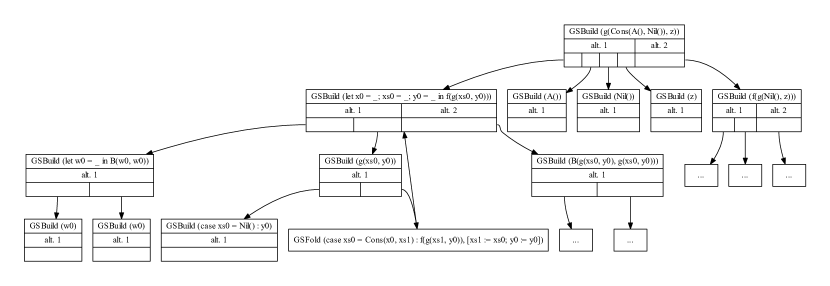
Figure 6: Partial Lazy Graph of “exp growth” Small Example

To illustrate the process on a very simple example, consider the example program from Fig. 7(f)-7(g) (explained in Sec. 4), but specialized to a smaller input: g(Cons(A, Nil), z). A part of the resulting lazy graph (omitting subgraphs for alternatives other than the first) is shown in Fig. 6. The full lazy graph for the same example is shown in the extended version of this article [12].

• Multi-result driving produces 2 alternatives from the initial expression g(Cons(A, Nil), z): let x0 = A; xs0 = Nil; y0 = z in f(g(xs0, y0)) and f(g(Nil, z)). As mentioned, we further consider only the subgraph for the first alternative, which is the result of a generalization.

• Driving cannot transform any further the subexpressions A, Nil, and z, so they end up as leafs in the lazy graph. Driving the subexpression f(g(xs0, y0)) again produces 2 alternatives: let w0 = g(xs0, y0) in B(w0, w0) and B(g(xs0, y0), g(xs0, y0)).

• The first alternative here has 2 subexpressions:

  • B(w0, w0), where driving of its subexpressions in turn leads to 2 leafs, both w0;

  • g(xs0, y0), where driving must perform a case analysis on x0, resulting in 2 subgraphs:

    • case xs0 = Nil() : y0, where driving cannot proceed any further;

    • case xs0 = Cons(x0, xs1) : f(g(xs1, y0)) – this expression is a renaming of f(g(xs0, y0)), encountered above, so we end up with a folding node.

4 Empirical Evaluation

We have studied the behavior of the proposed multi-result supercompiler on a few simple examples, with a focus on the resulting program size. A straightforward approach, which works for some of the smaller examples, is to enumerate all resulting configuration graphs and gather statistics from them. For one example – the well-known “KMP test” – this approach turned out to be too time consuming. So, to make it possible to analyze larger examples, we adapted the approach of Grechanik et al. [3], which permits to filter the sequence of configuration graphs produced by MRSC, without explicitly enumerating them. In particular, we have implemented functions to extract:

• the first configuration graph in the sequence (recall that by the ordering of results during driving, it should contain the most generalizations);

• the last one – with the least number of generalizations;

• the graph with the smallest number of nodes;

• the graph with the largest number of nodes.

The implementation of some of these functions is shown in the extended version of this article [12]. These implementations take polynomial time (and often almost linear time in practice) with respect to the size of the lazy graph, while the number of configuration graphs can be exponential with respect to this size. As such, they are key to making the proposed approach tractable on larger examples. By comparing the first to the smallest and the largest graph we can see how successful the proposed generalization strategy is in controlling code size. By comparing the last to the first and the smallest graph, we can see the improvements that our approach can achieve with respect to standard supercompilation – as the last configuration graph usually corresponds to the one that a standard positive supercompiler would produce.

After we extract a single configuration graph out of the lazy graph, we can further produce a new program in the object language from this graph. This residualization process involves 2 main steps: 1) Extract a program in a language extended with case and let expressions from the configuration graph. This step also creates recursive function definitions from fold nodes. 2) Remove case and let expressions (by a method similar to lambda lifting) to obtain a program in the original object language. The residualization process also includes several optimizations: a) removing “trivial” let expressions (expressions of the form let x = y in ..., or where the variable is only used once); b) removing duplicated function definitions (a limited form of common subexpression elimination). The results shown in Fig. 8-12 are all produced by applying this residualization process on the given configuration graph. Note, however, that we have decided to compare the sizes of the configuration graphs, and not of the residualized programs, for a couple of reasons:

• The size of the resulting program depends not only on the optimizations performed by supercompilation proper (which are reflected directly in the configuration graph), but also on the additional optimizations performed during residualization. The latter are standard optimizations that can be performed on any program, no matter if it is produced by supercompilation or written by hand.

• As already mentioned, we can efficiently extract a configuration graph of optimum size from the lazy graph. We have no way to do the same with respect to the size of the residual program.

⬇

append(Nil, ys) = ys;

append(Cons(x, xs), ys) = Cons(x, append(xs, ys));

(a) List Append Program

⬇

append(append(xs, ys), zs)

(b) Double Append

⬇

not(True) = False;

not(False) = True;

eqBool(True, b) = b;

eqBool(False, b) = not(b);

match(Nil, ss, op, os) = True;

match(Cons(p, pp), ss, op, os) = matchCons(ss, p, pp, op, os);

matchCons(Nil, p, pp, op, os) = False;

matchCons(Cons(s, ss), p, pp, op, os) = matchHdEq(eqBool(p, s), pp, ss, op, os);

matchHdEq(True, pp, ss, op, os) = match(pp, ss, op, os);

matchHdEq(False, pp, ss, op, os) = next(os, op);

next(Nil, op) = False;

next(Cons(s, ss), op) = match(op, ss, op, ss);

isSublist(p, s) = match(p, s, p, s);

(c) Substring Program

⬇

isSublist(Cons(True, Cons(True, Cons(False, Nil))), s)

(d) “KMP Test”

⬇

eqBool(eqBool(x, y), eqBool(y, x))

(e) Bool Equality Symmetry

⬇

g(Nil, y) = y;

g(Cons(x, xs), y) = f(g(xs, y));

f(w) = B(w, w);

(f) Program Demonstrating Exponential Growth

⬇

g(Cons(A, Cons(A, Cons(A, Nil))), z)

(g) Expression Demonstrating Exponential Growth

Figure 7: Example Programs

Here we analyze in detail several of the example programs (Fig. 7) showing the most interesting results. The extended version of this article [12] discusses a few additional examples.

• “double append” (Fig. 7(a)-7(b)) is traditionally used to demonstrate the power of deforestation and supercompilation. It can also be seen as a first step of a proof that list append is associative.

• The “KMP test” (Fig. 7(c)-7(d)) is another classical example, which demonstrates the power of supercompilation with respect to deforestation and partial evaluation. It involves specializing a sublist predicate to a fixed sublist being searched in an unknown list.

• “eqBool symmetry” (Fig. 7(c), 7(e)) is intended to show that Boolean equality is symmetric.

• “exp growth” (Fig. 7(f)-7(g)) is an example taken from Sørensen’s thesis [16, Example 11.4.1], who attributes it to Sestoft. It is aimed to demonstrate how classical supercompilation can produce output programs, which grow exponentially with respect to the input.

The results of the multi-result supercompilation – using our specific generalization approach – are summarized in Table 1. We give the configuration graph sizes for each of the four types of results (first, last, minimum/maximum size).

Table 1: MRSC Statistics
(Configuration graph sizes)

Example	First	Last	Min. size	Max. size
double append	12	10	10	19
KMP test	203	39	38	1055
eqBool symmetry	16	17	16	30
exp growth	15	37	15	57

Several interesting observations arise from analyzing the selected resulting programs themselves:

• In 2 cases (“eqBool symmetry” and “exp growth”) the minimum program coincides with the first (most generalizing) one; in 1 case (“double append”) – with the last (least generalizing) result. In “KMP test” the difference between the minimum-size and the last program is minimal. This confirms the highly unpredictable impact of driving+generalization on program size.

• Note, however, that “double append” is a bit of an outlier – it results in only 3 programs, one of which (the first) is isomorphic to the input. The smallest one is the expected optimized version, shown in Fig. 8.

• In all cases, the size of the first result is closer to the minimum than to the maximum size. This confirms that our choice of generalization ensures limited growth of the result size.

• The smallest/last “KMP test” graph produces the expected optimal (as execution time) program, as shown in Fig. 9.

• The last “eqBool symmetry” graph produces a program, which can indeed serve as evidence of the symmetry of Boolean equality – Fig. 10.

• The results of “exp growth” are especially interesting in view of our main goal. The last result is the same as produced by Sørensen’s supercompiler – B(B(B(z, z), B(z, z)), B(B(z, z), B(z, z))) – clearly suffering from code-size explosion. The minimum-size (and also first) program – shown in Fig. 11 – avoids the pitfall of code-size explosion, thanks to generalization. It has, however, also missed some opportunities for static evaluation. Interestingly, if we analyze the full set of results, there is another graph of size 17 that produces a program, which has eliminated all possible static reductions, while avoiding the risk of code explosion – Fig. 12. Apparently, if we do not want to miss such results, we need a more refined approach for looking for (close to) minimum-size programs. One explanation of this discrepancy is that – as already explained – rather than comparing the sizes of the programs produced by residualizing these graphs, we compare configuration graph sizes. A possible compromise is to study better size measures for configuration graphs, instead of the simple node count we currently use. For example, ignoring unfolding nodes when calculating size can give a better idea of the expected size of the residualized program, as unfolding nodes are skipped during residualization. Another possibility is to find not only (one of) the minimum-size result(s), but the $N$ smallest results ($N$ being an input parameter).

Based on the last observation above, we have implemented modified queries for finding the graph of minimum (and maximum) size, where unfolding nodes are not counted – with very encouraging results:

• for “double append”, “KMP test”, and “eqBool symmetry” the modified query returns the same optimal programs discussed above, which were also found by the existing queries for minimum or last program;

• for “exp growth”, the modified-minimum query again finds the optimal program – shown Fig. 12 – which was missed by all standard queries.

⬇

f_0(ys, zs) = f_0_case0(ys, zs);

f_0_case0(Nil(), zs) = zs;

f_0_case0(Cons(x0, xs0), zs) = Cons(x0, f_0(xs0, zs));

f_(xs, ys, zs) = f__case0(xs, ys, zs);

f__case0(Nil(), ys, zs) = f_0(ys, zs);

f__case0(Cons(x00, xs00), ys, zs) = Cons(x00, f_(xs00, ys, zs));

expression: f_(xs, ys, zs)

Figure 8: Optimized double-append

⬇

f_1_0_0_0_1_0_0(s0, ss1) = f_1_0_0_0_1_0_0_case0(s0, ss1);

f_1_0_0_0_1_0_0_case0(True(), ss1) = f_1_0_0_0_1_0_0_case1(ss1);

f_1_0_0_0_1_0_0_case0(False(), ss1) = f_0(ss1);

f_1_0_0_0_1_0_0_case1(Nil(), ) = False();

f_1_0_0_0_1_0_0_case1(Cons(s0, ss0), ) = f_1_0_0_0_1_0_0_case2(s0, s0, ss0);

f_1_0_0_0_1_0_0_case2(True(), s0, ss0) = f_1_0_0_0_1_0_0(s0, ss0);

f_1_0_0_0_1_0_0_case2(False(), s0, ss0) = True();

f_0(s) = f_0_case0(s);

f_0_case0(Nil(), ) = False();

f_0_case0(Cons(s0, ss0), ) = f_0_case1(s0, ss0);

f_0_case1(True(), ss0) = f_0_case2(ss0);

f_0_case1(False(), ss0) = f_0(ss0);

f_0_case2(Nil(), ) = False();

f_0_case2(Cons(s0, ss1), ) = f_1_0_0_0_1_0_0(s0, ss1);

expression: f_0(s)

Figure 9: Optimized KMP Test Result

⬇

main_case0(True(), y) = main_case2(y);

main_case0(False(), y) = main_case2(y);

main_case2(True(), ) = True();

main_case2(False(), ) = True();

expression: main_case0(x, y)

Figure 10: “eqBool symmetry” Optimal Result

⬇

f_3(xs0, y0) = f_3_let0(f_3_case0(xs0, y0));

f_3_let0(w0) = B(w0, w0);

f_3_case0(Nil(), y0) = y0;

f_3_case0(Cons(x0, xs1), y0) = f_3(xs1, y0);

expression: f_3(Cons(A(), Cons(A(), Nil())), z))

Figure 11: “exp growth” Minimum-size Result

⬇

main_let1(w0) = B(w0, w0);

expression: main_let1(main_let1(B(z, z)))

Figure 12: “exp growth” Optimal Result

5 Related Work

The unpredictability of supercompilation with respect to both performance and result size is a well-established issue. Problems with code duplication and result size are discussed by Sørensen [16], for example. Few works directly tackle this problem, however. Bolingbroke et al. [2] study heuristics for improving the general performance of a specific supercompiler, in order to use it as an automatic phase of an optimizing compiler for Haskell. Some of these heuristics concern avoiding code duplication, and as a consequence they may lead to improvements in result size, while still producing faster programs. The key idea is to roll back – discarding some work done by the supercompiler – if the heuristics indicate that this work is not leading to a useful result (a form of generalization). Speculative execution can also help with code size in some instances. One problem with this approach is that it is not clear how to generalize it or apply it to a completely different supercompiler. The main advantage is that by carefully selecting heuristics, suitable for the specific supercompiler, the authors report good results on a number of benchmarks.

Jonsson et al. [6] explicitly address both the issue of code explosion and the related issue of supercompilation time. The main idea is again to discard the result of supercompiling certain program fragments if they do not meet certain usefulness criteria (based on the number of reductions performed by the supercompiler and the resulting code size). We can again consider this a form of generalization. When such generalization happens, however, is based on specific hand-picked heuristics, apparently based on analyzing the results of different test runs.

Grechanik et al. [3] propose a generic framework for building “big-step” multi-result supercompilers, and a way to efficiently extract results satisfying certain criteria. Selecting the smallest result is one of the criteria studied. Optimization of the result size is not a goal of their work, however. The authors have instantiated the framework on a language simulating counter systems, which is not Turing-complete, and thus does not demonstrate some of the complications coming with Turing-complete object languages. The work of Grechanik et al. [3] is most closely related to ours: we re-use the ideas for implementing our multi-result supercompiler and for efficiently filtering its results by criteria. Our main emphasis, however, is on using MRSC together with a generalization strategy, which is explicitly tailored towards avoiding code duplication and – consequently – optimizing result size. We pay much less attention to supercompilation time, as long as it is not unacceptably big even for the small examples we want to analyze.

6 Conclusions and Future Work

We have presented a study on the feasibility of controlling result size after supercompilation – based on using multi-result supercompilation coupled with a specific generalization strategy avoiding code duplication. While the idea of multi-result supercompilation is not new, the idea to use it – combined with a specific generalization strategy – for taming code explosion in supercompilation results appears new. The current results of the approach – based on a small set of typical supercompilation examples – are encouraging:

• the smallest configuration graphs we produce do not show exponential growth with respect to the size of the input and typically are much smaller than the largest results;

• often the results of small size (though not necessarily the smallest) also feature a significant number of optimizations, comparable to what a standard classical supercompiler can achieve on the same task.

We have already hinted at some areas for potential improvements of the proposed approach:

• study less conservative definitions of generalization; for example, avoid generalizing expressions, which will not be duplicated (because the corresponding function parameter is not referenced multiple times), or expressions, whose duplication is not critical;

• study definitions of configuration graph size, which more closely match the expected size of the residualized program, to avoid missing interesting results, as was the case with “exp growth”.

Clearly the first thing to do, however, is to test the proposed approach on a larger set of different examples. Due to the small number of analyzed examples, we consider the current proposal to be work in progress. An extended set of tests could give more insight on the strengths and weaknesses of the proposed technique, and would likely lead to ideas for further study.

Provided we obtain mostly encouraging results from further testing, the next logical step would be to make the approach more practical:

• make an implementation covering a larger object language, closer to functional languages actually used in practice;

• provide a larger set of functions for quickly filtering useful results.

From a more theoretical perspective, it would be interesting to try to formulate properties of generalization, which can give some upper bounds on the code size of MRSC results. Because of unfolding, which can replace the current configuration with a new one of unrelated size (even if we avoid code duplication at this point), the task is not trivial. On the other hand, at least in the case of our simple object language, we have a fixed list of function definitions, which can give us some bound on the configuration size after unfolding.

Acknowledgments

The author would like to thank the four anonymous reviewers for the helpful suggestions on improving the presentation of this article.

References

- [1]
- [2] Max Bolingbroke & Simon Peyton Jones (2011): Improving supercompilation: tag-bags, rollback, speculation, normalisation, and generalisation. In: ICFP. Available at https://www.microsoft.com/en-us/research/publication/improving-supercompilation-tag-bags-rollback-speculation-normalisation-and-generalisation/.
- [3] Sergei Grechanik, Ilya Klyuchnikov & Sergei Romanenko (2014): Staged Multi-Result Supercompilation: Filtering by Transformation. In Andrei Klimov & Sergei Romanenko, editors: Proceedings of the Fourth International Valentin Turchin Workshop on Metacomputation, University of Pereslavl Publishing House, Pereslavl-Zalessky, Russia, pp. 54–78. Available at http://meta2014.pereslavl.ru/papers/2014_Grechanik_Klyuchnikov_Romanenko__Staged_Multi-Result_Supercompilation__Filtering_by_Transformation.pdf.
- [4] G. W. Hamilton (2007): Distillation: Extracting the Essence of Programs. In: Proceedings of the 2007 ACM SIGPLAN Symposium on Partial Evaluation and Semantics-Based Program Manipulation, PEPM ’07, Association for Computing Machinery, New York, NY, USA, pp. 61–70, 10.1145/1244381.1244391.
- [5] Neil D. Jones, Carsten K. Gomard & Peter Sestoft (1993): Partial Evaluation and Automatic Program Generation. Prentice-Hall, Inc., Upper Saddle River, NJ, USA.
- [6] Peter A. Jonsson & Johan Nordlander (2011): Taming Code Explosion in Supercompilation. In: Proceedings of the 20th ACM SIGPLAN Workshop on Partial Evaluation and Program Manipulation, PEPM ’11, Association for Computing Machinery, New York, NY, USA, pp. 33–42, 10.1145/1929501.1929507.
- [7] Ilya Klyuchnikov & Dimitur Krustev (2014): Supercompilation: Ideas and methods. The Monad Reader 23.
- [8] Ilya Klyuchnikov & Sergei Romanenko (2010): Proving the Equivalence of Higher-Order Terms by Means of Supercompilation. In Amir Pnueli, Irina Virbitskaite & Andrei Voronkov, editors: Perspectives of Systems Informatics: 7th International Andrei Ershov Memorial Conference, PSI 2009, Novosibirsk, Russia, June 15-19, 2009. Revised Papers, Springer Berlin Heidelberg, Berlin, Heidelberg, pp. 193–205, 10.1007/978-3-642-11486-117.
- [9] Ilya Klyuchnikov & Sergei A. Romanenko (2012): Multi-result Supercompilation as Branching Growth of the Penultimate Level in Metasystem Transitions. In Edmund Clarke, Irina Virbitskaite & Andrei Voronkov, editors: Perspectives of Systems Informatics, Springer Berlin Heidelberg, Berlin, Heidelberg, pp. 210–226, 10.1007/978-3-642-29709-019.
- [10] Ilya G. Klyuchnikov & Sergei A. Romanenko (2010): Towards Higher-Level Supercompilation. In A. P. Nemytykh, editor: Proceedings of the Second International Workshop on Metacomputation (META 2010), pp. 82–101.
- [11] Ilya G. Klyuchnikov & Sergei A. Romanenko (2012): Formalizing and Implementing Multi-Result Supercompilation. In A. V. Klimov & S. A. Romanenko, editors: Proceedings of the Third International Workshop on Metacomputation (META 2012), pp. 142–164.
- [12] Dimitur Krustev (2020): Controlling the Size of Supercompiled Programs using Multi-result Supercompilation. Available at https://arxiv.org/abs/2006.02204.
- [13] Dimitur Nikolaev Krustev (2014): An Approach for Modular Verification of Multi-Result Supercompilers. In A.V. Klimov & S.A. Romamenko, editors: Proceedings of the Fourth International Valentin Turchin Workshop on Metacomputation, University of Pereslavl Publishing House, Pereslavl-Zalessky, Russia, pp. 177–193.
- [14] Alexei P. Lisitsa & Andrei P. Nemytykh (2017): Verification of Programs via Intermediate Interpretation. Electronic Proceedings in Theoretical Computer Science 253, pp. 54–74, 10.4204/eptcs.253.6.
- [15] Gavin Mendel-Gleason (2011): Types and Verification for Infinite State Systems. PhD thesis, Dublin City University, Dublin, Ireland.
- [16] M. H. Sørensen (1994): Turchin’s Supercompiler Revisited: an Operational Theory of Positive Information Propagation. Master’s thesis, Københavns Universitet, Datalogisk Institut.
- [17] Morten Heine Sørensen & Robert Glück (1999): Introduction to Supercompilation. In John Hatcliff, Torben Mogensen & Peter Thiemann, editors: Partial Evaluation: Practice and Theory, Lecture Notes in Computer Science 1706, Springer-Verlag, pp. 246–270, 10.1007/3-540-47018-210.
- [18] Valentin F. Turchin (1986): The Concept of a Supercompiler. ACM Trans. Program. Lang. Syst. 8(3), pp. 292–325, 10.1145/5956.5957.