S2OSC: A Holistic Semi-Supervised Approach for Open Set Classification

Abstract

Open set classification (OSC) tackles the problem of determining whether the data are in-class or out-of-class during inference, when only provided with a set of in-class examples at training time. Traditional OSC methods usually train discriminative or generative models with in-class data, then utilize the pre-trained models to classify test data directly. However, these methods always suffer from embedding confusion problem, i.e., partial out-of-class instances are mixed with in-class ones of similar semantics, making it difficult to classify. To solve this problem, we unify semi-supervised learning to develop a novel OSC algorithm, S2OSC, that incorporates out-of-class instances filtering and model re-training in a transductive manner. In detail, given a pool of newly coming test data, S2OSC firstly filters distinct out-of-class instances using the pre-trained model, and annotates super-class for them. Then, S2OSC trains a holistic classification model by combing in-class and out-of-class labeled data and remaining unlabeled test data in semi-supervised paradigm, which also integrates pre-trained model for knowledge distillation to further separate mixed instances. Despite its simplicity, the experimental results show that S2OSC achieves state-of-the-art performance across a variety of OSC tasks, including $85.4\%$ of F1 on CIFAR-10 with only 300 pseudo-labels. We also demonstrate how S2OSC can be expanded to incremental OSC setting effectively with streaming data.

1 Introduction

The real-world is changing dynamically, and many applications are non-stationary, which always receive the data containing out-of-class (also called unknown class) instances, for example, self-driving cars need to identify unknown objects, face recognition system needs to distinguish unseen personal pictures, image retrieval often emerges new categories, etc. This problem is defined as “Open Set Classification (OSC)” in literature [1]. Different from traditional Closed Set Classification (CSC) which assumes training and testing data are draw from same spaces, i.e., the label and feature spaces, OSC aims to not only accurately classify in-class (also called known class) instances, but also effectively detect out-of-class instances. Besides, a generalized situation is that out-of-class instances will arise continuously with the streaming data, i.e., unknown classes appear incrementally, which is also defined as incremental OSC.

Both anomaly detection [2, 3] and zero-shot learning [4, 5] are related to open set classification. They have similar objectives to detect anomaly/out-of-class instances given a set of in-class examples. In contrast, anomaly detection (also called outlier detection) is an unsupervised learning task [3]. The goal is to separate abnormal in-class instances from normal ones, where the distinction from OSC is that differences between unknown and known classes are larger than that between anomalies and known classes [6]. Unlike anomaly detection, zero-shot learning (ZSL) focuses on constructing related OSC models to address unknown class detection issue, which merely utilize in-class examples and semantic information about unknown classes. Whereas the standard ZSL methods only test out-of-class instances, rather than test both known and unknown classes. Thus, generalized zero-shot learning (GZSL) is proposed, which automatically detect known and unknown classes simultaneously. For example, [4, 5] learned more reliable classification models by measuring the distance between examples and corresponding in-class/out-of-class semantic embeddings. However, both ZSL and GZSL assume that semantic information (for example, attributes or descriptions) of the unknown classes is given, which is limited to classify with prior knowledge.

Therefore, a more realistic classification is to detect out-of-class without any information of unknown classes. With the advent of deep learning, recent OSC approaches can mainly be divided into two aspects: discriminative and generative models. Discriminative models mainly utilize the powerful feature learning and prediction capabilities of deep models to design corresponding distance or prediction confidence measures [7, 8]. In contrast, generative models mainly employ the adversarial learning to generate out-of-class instances near the decision margin that can fool the discriminative model [9, 10]. In summary, existing OSC approaches focus on learning a representative latent space for in-class examples that preserves details of the given classes. In this case, it is assumed that when presents out-of-class instances to the pre-trained network, it will generate a poor embedding that reports a relatively higher classification error. However, this assumption does not hold for all situations. For example, as shown in Figure 1, experiments on MNIST suggest that networks (discriminative and generative models [8, 11]) trained with simple content have high novelty detection accuracy, i.e., the embeddings of out-of-class digits 5 and 6 are well separated from in-class examples. In contrast, instances with complex content, such as CIFAR-10, have much low novelty detection accuracy. This is because latent embeddings learned for in-class examples can also inherently apply to represent some out-of-class instances, for example, the latent embeddings learned for cat (number $3$ in Figure 1 (b) and (d)) are also able to represent some instances of other out-of-class animal such as dog (number $5$ in Figure 1 (b) and (d)), considering similar appearance, color and other information. This phenomenon is defined as Embedding Confusion in this paper.

We note that out-of-class instances always include confused and distinct ones. Thereby we can firstly select the distinct out-of-class instances, then re-train a new classifier by combing stored in-class examples in semi-supervised paradigm. Meanwhile, the pre-trained model can be employed as a teacher model, which not only ensures that in-class instances are well represented, but also guarantees that out-of-class instances are poorly represented. In result, the learned classifier can obtain well separated embeddings for in-class and out-of-class instances, and significantly improve the detection performance in return. Motivated by this intuition, we propose Semi-Supervised Open Set Classification algorithm (S2OSC), a transductive classifier learning process to mitigate embedding confusion. To the best of our knowledge, none of the previous work has addressed this detection manner. At a high-level, S2OSC can also be adapted to incremental OSC conveniently.

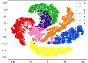
(a) DM on MNIST

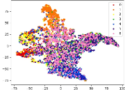
(b) DM on CIFAR-10

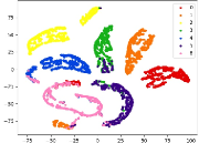
(c) GM on MNIST

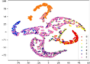
(d) GM on CIFAR-10

Figure 1: T-SNE of discriminative model (DM) [8] and generative model (GM) [11] on simple (MNIST) and complex (CIFAR-10) datasets. We develop these two models with five classes (i.e., 0-4) in training stage according to the raw paper, then utilize the pre-trained models to achieve the embeddings of known classes (i.e., 0-4) and unknown classes (i.e., 5 and 6) appearing in testing stage. Note that traditional OSC methods usually classify based on the learned embeddings.

2 Related Work

To set forth the S2OSC, we first introduce existing methods for OSC, which are related to our S2OSC, i.e., discriminative and generative models. Then we present traditional anomaly detection and zero-shot learning methods.

Discriminative OSC models. These approaches mainly restrict intra-class and inter-class distance property on training data, and detect unknown classes by identifying outliers. For example, [12] developed a SVM-based method, which learned the concept of known classes while incorporating the structure presented in unlabeled data from open set; [13] proposed to dynamically maintain two low-dimensional matrix sketches to detect emerging new classes. However, these linear approaches are difficult to process high dimensional space. Recently, several studies have applied deep learning techniques to OSC scenario. For example, [7] distinguished known/unknown class with softmax output probabilities; [14] directly utilized temperature scaling to separate the softmax score between in-distribution and out-of-distribution images; [8] proposed a cnn-based prototype ensemble method, which adaptively updates prototype for robust detection. However, these methods can hardly consider the out-of-class instances in training phase.

Generative OSC models. The key component of generation-based OSC models is to generate effective out-of-class instances. For example, [9] proposed the generative OpenMax (G-OpenMax) algorithm, which provides probability estimation over generated out-of-class instances, that enables the classifier to locate the decision margin according to both in-class and out-of-class knowledge; [10] adopted the GAN technique to generate fake data considering representativeness as the out-of-class data, which can further enhance the robustness of classifier for detection; [11] introduced an augmentation technique, which adopts an encoder-decoder GAN architecture to generate synthetic instances similar to known classes. Though these methods have achieved some improvements, generating more effective out-of-class instances with complex content still need further research [11].

Traditional detection models. Anomaly detection and generalized zero-shot learning are also related to OSC task. The goal of anomaly detection is to separate outlier instances, for example, [2] proposed a non-parametric method IForest, which detects outliers with ensemble trees. However, anomaly detection follows different protocols from OSC methods, and unable to subdivide known classes. Generalized zero-shot learning aims to classify known and unknown classes with side information. For example, [4] employed manifold learning to align semantic space with visual features; [5] introduced the feature confusion GAN, which adopts a boundary loss to maximize the margin of known and unknown classes. However, they assume that semantic information of unknown classes is already in existence, which is incomparable with OSC methods.

3 Our Algorithm: S2OSC

3.1 Problem Definition

Without any loss of generality, suppose we have a supervised training set $\mathcal{D}_{tr}=\{({\bf x}_{i},{\bf y}_{i})\}_{i=1}^{N_{tr}}$ at initial time, where ${\bf x}_{i}\in\mathcal{R}^{d}$ denotes the $i-$th instance, and ${\bf y}_{i}\in Y=\{1,2,\cdots,C\}$ denotes the corresponding label. Then, we receive a pool of unlabeled testing data $\mathcal{D}_{te}=\{({\bf x}_{j})\}_{j=1}^{N_{te}}$, where ${\bf x}_{j}\in\mathcal{R}^{d}$ denotes the $j-$th instance, and label ${\bf y}_{j}\in\hat{Y}=\{1,2,\cdots,C,C+1,\cdots,C+B\}$ is unknown. $\{1,2,\cdots,C\}$ denotes in-class set and $\{C+1,\cdots,C+B\}$ represents out-of-class set. Therefore, open set classification can be defined as:

Definition 1

Open Set Classification (OSC) With the initial training set $\mathcal{D}_{tr}=\{({\bf x}_{i},{\bf y}_{i})\}_{i=1}^{N_{tr}}$, we aim to construct a model $f:X\rightarrow Y$. Then with the pre-trained model $f$, OSC is to classify the in-class and out-of-class instances in $\mathcal{D}_{te}$ accurately.

Following most OSC approaches [12, 13, 11, 14, 8, 1], we firstly consider all unknown classes as a super-class for detection, then employ unsupervised clustering techniques such as k-means for subdividing (out-of-class specifically refers to super-class in following). Therefore, given the $f$ and $\mathcal{D}_{te}$, we transform to build a new classifier $g$ in transductive manner for operating OSC on $\mathcal{D}_{te}$. In detail, S2OSC pre-trains a classification model $f$ with $\mathcal{D}_{tr}$ and stores limited in-class examples $\mathcal{D}_{in}$ from $\mathcal{D}_{tr}$. $f$ is then used for filtering distinct out-of-class instances $\mathcal{D}_{out}$ in $\mathcal{D}_{te}$. After this, we possess in-class and potential out-of-class labeled data $\mathcal{X}=\{\mathcal{D}_{in},\mathcal{D}_{out}\}$, and unlabeled data $\mathcal{U}=\{\mathcal{D}_{te}\setminus\mathcal{D}_{out}\}$, thereby we can develop a new classifier $g$ in semi-supervised paradigm. Note that there are two ways to train $g$: 1) fine-tuning based on $f$ directly; 2) retraining from scratch while using $f$ as a teacher for knowledge distillation. We select the second way considering the efficiency and effectiveness. Consequently, we acquire the classification results of $\mathcal{D}_{te}$ using learned $g$ in a transductive manner. In fact, S2OSC comprehensively considers the ideas of both discriminant and generative methods, i.e., trying to separate known classes as far as possible, while taking into account the potential information of unknown classes. Next, we describe each part of S2OSC.

3.2 Data Filtering

With the initial in-class training data $\mathcal{D}_{tr}$, we firstly develop a deep classification model $f$ as many typical supervised methods:

$$\begin{split}f^{*}=\arg\min\limits_{f}\sum_{i=1}^{N_{tr}}\ell({\bf y}_{i},f({\bf x}_{i}))\end{split}$$ (1)

$\ell$ can be any convex loss function, and we define as cross-entropy loss for unification here. Meanwhile, we randomly select $K$ examples from each class to constitute $\mathcal{D}_{in}$. Then, we evaluate the weight of each instance in $\mathcal{D}_{te}$ by self-taught weighting function. In detail, we compute confidence score for each instance ${\bf x}_{j}$ in $\mathcal{D}_{te}$ using pre-trained model $f^{*}$:

$$\begin{split}w_{j}=u_{j}+\lambda d_{j}\end{split}$$ (2)

where $\lambda$ is a fixed hyperparameter. $u_{j}$ denotes statistic prediction confidence, which is done explicitly with the entropy: $u_{j}=-\sum_{c}f_{c}^{*}({\bf x}_{j})\log f_{c}^{*}({\bf x}_{j})$. $d_{j}$ represents statistic distance to each in-class center, i.e., $d_{j}=\min(\|e_{j}-\mu_{c}\|_{2}^{2})$, where $e_{j}$ represents embeddings extracted from feature output layer of $f^{*}$, and $\mu_{c}=\frac{1}{|\mathcal{D}^{c}_{tr}|}\sum_{{\bf x}\in\mathcal{D}^{c}_{tr}}e_{{\bf x}}$ represents $c-$th in-class center, $\mathcal{D}^{c}_{tr}$ is $c-$th class set. It is notable that highly unsure out-of-class instances have larger weights, while in-class and confused instances have lower weights. In result, we can sort $\mathcal{D}_{te}$ according to $w$, and acquire filtered instances set $\mathcal{D}_{out}$ with the same number $K$ as in-class set, the corresponding super-class is $C^{\prime}$. Therefore, we have owned in-class and out-of-class labeled data $\mathcal{X}=\{\mathcal{D}_{in},\mathcal{D}_{out}\}$, unlabeled data $\mathcal{U}=\{\mathcal{D}_{te}\setminus\mathcal{D}_{out}\}$, and aim to develop the new classifier $g$.

3.3 Objective Function

Inspired from [15], we combine two common semi-supervised methods to learn $g$: consistency regularization and pseudo-labeling, which aim to effectively utilize unlabeled data by ensuring the consistency among different data-augmented forms. S2OSC has two contributions: 1) Pseudo-labeling threshold. For a given unlabeled instance, the pseudo-label is only retained if $g$ produces a high-confidence prediction; 2) Pre-trained model teaching. For a given instance, we use the pre-trained model $f$ for knowledge distillation of predictions from known classes. Therefore, we can further separate the confused out-of-class instances with in-class instances.

Specifically, the loss function of $g$ exclusively consists of two terms: a supervised loss $L_{s}$ applied to labeled data and an unsupervised loss $L_{u}$. $L_{s}$ can be represented as:

$$\begin{split}L_{s}=&\frac{1}{2|\mathcal{X}|}\sum_{l=1}^{|\mathcal{X}|}(\ell_{s1}({\bf x}_{l},{\bf y}_{l})+\alpha\ell_{s2}({\bf x}_{l},f^{*}({\bf x}_{l})))\\ \ell_{s1}=&H_{in}({\bf y}_{l},g({\bf x}_{l}))+{\bf 1}_{max(g({\bf x}_{l}))\geq\tau}H_{out}({\bf y}_{l},g({\bf x}_{l}))\\ \ell_{s2}=&KL(f^{*}({\bf x}_{l})\|g_{\setminus C^{\prime}}({\bf x}_{l}))\end{split}$$ (3)

where $H_{(\cdot)}(p,q)=-p\log q$ is standard cross-entropy loss, $KL(p\|q)=p\log\frac{p}{q}$ denotes KL-divergence. $\alpha$ is a hyperparameter, $\tau$ is a scalar parameter denoting the threshold. $g_{\setminus C^{\prime}}({\bf x}_{l})$ is the prediction distribution with re-softmax except out-of-class $C^{\prime}$. $\ell_{s1}$ adopts the standard cross-entropy loss, note that there may still have embedding confused known class data in $\mathcal{D}_{out}$, thus we utilize ${\bf 1}_{max(g({\bf x}_{l}))\geq\tau}$ term to produce a valid “one-hot” probability distribution. Meanwhile, ideally, for labeled known class data in $\mathcal{X}$, $f$ can also produce confident probability distribution, otherwise $f$ tends to predict uniform distribution. Thus, $\ell_{s2}$ receives the soft targets from $f$ for in-class and out-of-class examples, which aim to proceed knowledge distillation by restraining two prediction distribution. $f^{*}({\bf x}_{l})$ and $g_{\setminus C^{\prime}}({\bf x}_{l})$ is with Softmax-T that sharpens distribution by adjusting its temperature $T$ following [16], i.e., raising all probabilities to a power of $\frac{1}{T}$ and re-normalizing.

For unlabeled data, S2OSC firstly obtains the pseudo-label by computing the prediction for a given unlabeled instance: $q_{u}=g({\bf x}_{u})$, and $\hat{q}_{u}=\arg\max(q_{u})$ is the pseudo-label, which is then used to enforce the loss against model’s output for a augmented version of ${\bf x}_{u}$:

$$\begin{split}L_{u}=&\frac{1}{2|\mathcal{U}|}\sum_{u=1}^{|\mathcal{U}|}{\bf 1}_{max(q_{u})\geq\tau}(\ell_{u1}({\bf x}_{u},\hat{q}_{u})+\alpha\ell_{u2}({\bf x}_{u},f^{*}({\bf x}_{u})))\\ \ell_{u1}=&H(\hat{q}_{u},g(\Phi({\bf x}_{u})))\\ \ell_{u2}=&KL(f^{*}({\bf x}_{u})\|g_{\setminus C^{\prime}}(\Phi({\bf x}_{u})))\end{split}$$ (4)

where $\tau$ denotes threshold above which we retrain the pseudo-label. $\Phi$ represents weak augmentation using a standard flip-and-shift strategy or strong augmentation using CTAugment [17] with Cutout [18] as [15], we employ the former strategy considering efficiency. See Appendix for details. $\ell_{u2}$ employs similar function on unlabeled data. Thus, $L_{u}$ encourage the model’s predictions to be low-entropy (i.e., high-confidence) on unlabeled data combing hard-label and soft-label. In summary, the loss minimized by S2OSC is: $L=L_{s}+\lambda_{u}L_{u}$, where $\lambda_{u}$ is a fixed scalar hyperparameter denoting the relative weight. Consequently, the trained $g$ can classify in-class or out-of-class instances in $D_{te}$, and then employ clustering on out-of-class instances to acquire sub-classes.

4 Incremental S2OSC (I-S2OSC)

In this section, we aim to demonstrate that S2OSC can be extended into incremental open set classification scenario conveniently.

4.1 Problem Definition

In real applications, we always receive the streaming data, and unknown classes are also emerge incrementally. Thus more generalized setting is incremental OSC, which has two characteristics: 1) Data pool. At time window $t$, we only get the data of current time window, i.e., $\mathcal{D}_{te}^{t}$, not full amount of previous data; 2) Unknown class continuity. At time window $t$, unknown classes appear partially, thereby we need to incrementally conduct OSC, i.e., every time after receiving the data of time window $t$, OSC is performed. Specifically, the streaming data $\mathcal{D}$ can be divided into $\mathcal{D}=\{\mathcal{D}^{t}\}_{t=0}^{T}$, where $\mathcal{D}^{0}=\mathcal{D}_{tr}$ is the initial training set. $\mathcal{D}^{t}=\{{\bf x}_{j}^{t}\}_{j=1}^{N_{t}},t\geq 1$ is with $N_{t}$ unlabeled instances, and the underlying label ${\bf y}_{j}^{t}\in\hat{Y}^{t}$ is unknown, $\hat{Y}^{t}=\hat{Y}^{t-1}\cup Y^{t}$, where $\hat{Y}^{t-1}$ is the cumulative known classes until $(t-1)-$th time window and $Y^{t}$ is the unknown class set in $t-$th window. Therefore, we provide the definition of incremental open set classification:

Definition 2

Incremental Open Set Classification (IOSC) At time $t\in\{1,2,\cdots,T\}$, we have pre-trained model $f^{t-1}$ and limited stored in-class examples $M^{t-1}$ until $(t-1)-$th time, then receive newly coming data pool $\mathcal{D}^{t}$. First, we aim to classify known and unknown classes in $\mathcal{D}^{t}$ as Definition 1. Then, with the labeled data from novel classes and stored data $M^{t-1}$, we update the model while mitigating forgetting to acquire $f^{t}$. Cycle this process until terminated.

S2OSC can be applied directly for OSC of $\mathcal{D}^{t}$ at $t-$th time window, then the extra challenge is to update the model while mitigating forgetting [19] of previous in-class knowledge.

4.2 Model Update

There exist two labeling cases after OSC, i.e., manually labeling and self-taught labeling [13]. We consider first setting following most approaches [1, 13, 8] to avoid label noise accumulation. In detail, after known/unknown classification operator, we can achieve potential out-of-class instances to query their true labels. However, there exist catastrophic forgetting of known classes if we only use the new data to update the model. To solve this problem, we employ a mechanism to incorporate the stored memory and novel class information incrementally, which can mitigate forgetting of discriminatory characteristics about known classes. Specifically, we utilize the exemplary data $M^{t-1}$ for regularization in fine-tuning:

$$\begin{split}L^{t}&=\sum_{l}\ell({\bf y}_{l},f^{t}({\bf x}_{l}))\\ s.t.&\quad\ell(M^{t-1},f^{t})\leq\ell(M^{t-1},f^{t-1})\end{split}$$ (5)

The loss term encourages the labeled unknown class examples to fine-tune $f^{t-1}$ for better performance, while constraint term imposes $M^{t-1}$ for less forgetting of old in-class knowledge. We utilize directly joint optimization on $M^{t-1}$ as iCaRL [20] to optimize variant of Eq. 5. See Appendix for details. After that, we need to update the $M^{t-1}$ to store key points of unknown classes. If $M^{t-1}$ is not full, we can fill selected instances from unknown class directly. Otherwise, we remove equal instances for each known class, and fill instances for each unknown class.

Table 1: Comparison of open set classification performance.

Methods	Accuracy					F1
	F-MN	CIFAR	SVHN	MN	CINIC	F-MN	CIFAR	SVHN	MN	CINIC
Iforest	.554	.243	.198	.632	.240	.553	.243	.197	.625	.240
One-SVM	.474	.260	.195	.537	.243	.671	.223	.102	.520	.206
LACU	.394	.325	.193	.695	.303	.409	.326	.091	.681	.268
SENC	.420	.215	.184	.358	.230	.489	.171	.124	.302	.166
ODIN	.563	.426	.601	.778	.329	.854	.380	.584	.767	.243
CFO	.639	.502	.663	.514	.389	.720	.514	.656	.513	.359
CPE	.628	.438	.645	.961	.246	.605	.353	.791	.960	.270
DTC	.576	.363	.534	.741	.388	.665	.495	.606	.717	.452
S2OSC	.972	.847	.898	.985	.785	.972	.854	.901	.985	.787

Methods	Precision					Recall
	F-MN	CIFAR	SVHN	MN	CINIC	F-MN	CIFAR	SVHN	MN	CINIC
Iforest	.553	.554	.252	.243	.198	.197	.657	.632	.245	.240
One-SVM	.671	.474	.286	.260	.195	.102	.616	.537	.274	.243
LACU	.409	.394	.331	.325	.193	.091	.676	.695	.363	.303
SENC	.489	.420	.253	.215	.184	.124	.448	.358	.211	.230
ODIN	.854	.563	.520	.426	.601	.584	.878	.778	.554	.329
CFO	.720	.639	.579	.502	.663	.656	.598	.514	.436	.389
CPE	.605	.698	.336	.408	.645	.791	.955	.961	.302	.316
DTC	.665	.576	.435	.463	.434	.606	.699	.681	.428	.388
S2OSC	.972	.972	.888	.847	.898	.901	.986	.985	.799	.785

5 Experiments

5.1 Datasets and Baselines

Considering that incremental OSC is an extension of OSC, the incremental OSC methods can also be applied to the setting of OSC. Therefore, we adopt commonly used incremental OSC datasets for validation here. In detail, we utilize five visual datasets in this paper following [8], i.e., FASHION-MNIST (F-MN) [21], CIFAR-10 (CIFAR) [22], SVHN [23], MNIST (MN) [24], CINIC . To validate the effectiveness of proposed approach, we compared it with existing state-of-the-art OSC and incremental OSC methods. First, we compare it with traditional anomaly detection and linear methods: Iforest [2], One-Class SVM (One-SVM) [25], LACU-SVM (LACU) [12], SENC-MAS (SENC) [13]. Second, we compare it with recent deep methods: ODIN-CNN (ODIN) [14], CFO [11], CPE [8] and DTC [27]. Abbreviations in parentheses. DTC is clustering based methods for multiple unknown classes detection. Note that Iforest, One-SVM, LACU, ODIN, CFO, and DTC are OSC methods, SENC and CPE are incremental OSC methods. All OSC baselines except Iforest can be updated incrementally using newly labeled unknown class data and memory data.

5.2 Open Set Classification

To rearrange each dataset for emulating a OSC form, we randomly hold out 50$\%$ classes as initial training set, and leave one class for testing. Experiments about OSC with various number of out-of-classes can refer to supplementary materials. Moreover, we extracted 33$\%$ of the known class data into test set, so that the test set mixes with known and unknown classes. Here we utilize four commonly used criteria, i.e., Accuracy, Precision, Recall and F1 (Weighted F1), to measure the classification performance, which considers all known and unknown classes. For example, accuracy $A=\frac{\sum_{i=1}^{|\hat{Y}|}(TP_{i}+TN_{i})}{\sum_{i=1}^{|\hat{Y}|}TP_{i}+TN_{i}+FP_{i}+FN_{i}}$, where $TP,FP,FN,TN$ denotes the true positives, false positive, false negatives and true negatives.

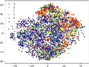
(a) Original

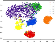
(b) S2OSC

Figure 2: T-SNE Visualization on CIFAR-10 dataset. (a) original feature space; (b) learned embeddings by proposed S2OSC.

Table 1 compares the classification performances of S2OSC with all baselines. We observe that: 1) outlier detection and linear methods perform poorly on most complex datasets, i.e., CIFAR-10, SVHN and CINIC, this indicates that they are difficult to process high dimensional data with complex content; 2) CNN-based methods are better than traditional OSC approaches, i.e., One-SVM, LACU, SENC. This indicates that neural network can provide better feature embeddings for prediction; 3) S2OSC consistently outperforms all baselines over various criteria by a significant margin. For example, in all datasets, S2OSC provides at least 20$\%$ improvements than baselines. This indicates the effectiveness of semi-supervised operation for mitigating embedding confusion. Figure 2 shows feature embedding results using T-SNE with the similar setting in Figure 1. Clearly, the figure (b) shows that the output of S2OSC has learned distinct groups, which is much better than original embeddings and corresponding embeddings of other deep methods in Figure 1. This validates that instances from unknown classes are well separated from other known clusters, which benefits for unknown class detection.

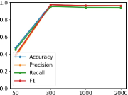
(a) Fashion-MNIST

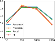
(b) CIFAR-10

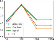
(c) SVNH

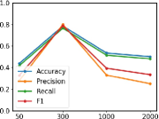
(d) CINIC

Figure 3: Classification performance with various number of filtered out-of-class instances.

Figure 3 shows the influence of important parameter $K$ (filtering size), i.e., we tune the size of $K=\{50,300,1000,2000\}$. The results reveal that, at first, different criteria improve with the increase of filtered instances. After filtering size is more than a threshold, the performance start to decrease. For example, on CIFAR-10, the accuracy on 300 filtering is about 84.7$\%$, yet the performance decreases after 300 filtering, this is due to the introduction of embedding confused instances with the increase of $K$.

Table 2: Comparison of incremental open set classification performance.

Methods	Average Accuracy					Average F1
	F-MN	CIFAR	SVHN	MN	CINIC	F-MN	CIFAR	SVHN	MN	CINIC
Iforest	.533	.221	.170	.606	.220	.489	.217	.162	.595	.217
One-SVM	.404	.218	.167	.471	.205	.409	.169	.085	.476	.156
LACU	.332	.199	.149	.171	.188	.267	.137	.052	.088	.114
SENC	.341	.197	.156	.296	.197	.264	.145	.100	.251	.138
ODIN	.780	.334	.625	.853	.276	.767	.284	.593	.850	.206
CFO	.659	.306	.485	.745	.291	.635	.304	.472	.722	.283
CPE	.618	.368	.695	.961	.286	.599	.343	.701	.960	.260
DTC	.586	.393	.514	.711	.348	.609	.445	.566	.717	.382
I-S2OSC	.818	.660	.771	.926	.567	.774	.609	.732	.913	.517

Methods	Average Precision					Average Recall
	F-MN	CIFAR	SVHN	MN	CINIC	F-MN	CIFAR	SVHN	MN	CINIC
Iforest	.498	.503	.226	.221	.166	.170	.621	.607	.225	.221
One-SVM	.597	.405	.216	.219	.187	.167	.672	.472	.210	.205
LACU	.262	.332	.133	.200	.043	.150	.266	.172	.143	.188
SENC	.330	.342	.207	.198	.210	.157	.390	.297	.197	.198
ODIN	.858	.781	.456	.334	.672	.626	.920	.853	.372	.276
CFO	.634	.659	.307	.306	.477	.486	.803	.745	.285	.291
CPE	.666	.619	.427	.368	.762	.696	.965	.961	.332	.286
DTC	.666	.586	.536	.394	.657	.515	.800	.711	.469	.349
I-S2OSC	.759	.818	.597	.661	.718	.771	.893	.922	.509	.568

Table 3: Forgetting measure of known classes over streaming data.

Methods	Forgetting
	Iforest	One-SVM	LACU	SENC	ODIN	CFO	CPE	DTC	I-S2OSC
F-MN	N/A	.139	.121	.127	.107	.047	.032	.055	.029
CIFAR	N/A	.202	.127	.172	.132	.128	.118	.120	.117
SVHN	N/A	.243	.330	.249	.168	.130	.124	.159	.123
MN	N/A	.141	.080	.061	.049	.040	.033	.044	.037
CINIC	N/A	.224	.227	.278	.170	.190	.147	.175	.138

5.3 Incremental Open Set Classification

Furthermore, we rearrange instances in each dataset to emulate a streaming form with incremental unknown classes as [8]. We utilize the same four criteria, i.e., average Accuracy, average Precision, average Recall and average F1, over various data pools to measure the performance following [8], which aims to calculate the overall performance for streaming data. Moreover, to validate the catastrophic forgetting of $f$, we calculate the performance about forgetting profile of different learning algorithms as [28], which defines the difference between maximum knowledge gained of emerging classes on a particular window throughout the learning process and we currently have about it, the lower difference the better.

Table 2 compares the classification performance of I-S2OSC with all baselines on streaming data. Table 3 compares the forgetting performance. “N/A” denotes no results considering that Iforest has no update process. We observe that: 1) comparing with results in Table 1, most average classification metrics of deep methods have improved while linear methods decreased, this indicates that deep models can still effectively distinguish known classes for streaming data, which can further benefit OSC; 2) I-S2OSC is superior than other baselines over accuracy and F1 metrics except MNIST dataset, and other two metrics are competitive. But it is not as obvious as the effect in OSC setting. Besides, the average performance of I-S2OSC decreases comparing OSC setting. These phenomenons are because that we uniformly set $K$ to 300, and with the increase of emerging classes, the number of inclusive in-class in filtering data also increases, which will affect the training of $g$. Thus the value of $K$ needs to be tuned carefully; 3) I-S2OSC has the smallest forgetting except MMIST dataset by considering exemplary regularization, which benefits to preserve known class knowledge.

6 Conclusion

Real-word applications always receive the data with unknown classes, thus it is necessary to promote the open set classification. The key challenge in OSC is to overcome the embedding confusion caused by out-of-class instances. To this end, we propose a holistic semi-supervised OSC algorithm, S2OSC. S2OSC incorporated out-of-class instances filtering and semi-supervised model training in a transductive manner, and integrated in-class pre-trained model for teaching. Moreover, S2OSC can be adapted to incremental OSC setting efficiently. Experiments showed the superior performances of S2OSC and I-S2OSC.

References

- [1] Geng, C., S. Huang, S. Chen. Recent advances in open set recognition: A survey. CoRR, abs/1811.08581, 2018.
- [2] Liu, F. T., K. M. Ting, Z. Zhou. Isolation forest. In ICDM, pages 413–422. 2008.
- [3] Xia, Y., X. Cao, F. Wen, et al. Learning discriminative reconstructions for unsupervised outlier removal. In ICCV, pages 1511–1519. 2015.
- [4] Changpinyo, S., W.-L. Chao, B. Gong, et al. Synthesized classifiers for zero-shot learning. In CVPR, pages 5327–5336. 2016.
- [5] Li, J., M. Jing, K. Lu, et al. Alleviating feature confusion for generative zero-shot learning. In ACMMM, pages 1587–1595. 2019.
- [6] Cai, X., P. Zhao, K. Ting, et al. Nearest neighbor ensembles: An effective method for difficult problems in streaming classification with emerging new classes. In ICDM, pages 970–975. 2019.
- [7] Hendrycks, D., K. Gimpel. A baseline for detecting misclassified and out-of-distribution examples in neural networks. In ICLR. 2017.
- [8] Wang, Z., Z. Kong, S. Chandra, et al. Robust high dimensional stream classification with novel class detection. In ICDE, pages 1418–1429. 2019.
- [9] Ge, Z., S. Demyanov, R. Garnavi. Generative openmax for multi-class open set classification. In BMVC. 2017.
- [10] Jo, I., J. Kim, H. Kang, et al. Open set recognition by regularising classifier with fake data generated by generative adversarial networks. In ICASSP, pages 2686–2690. 2018.
- [11] Neal, L., M. L. Olson, X. Z. Fern, et al. Open set learning with counterfactual images. In ECCV, pages 620–635. 2018.
- [12] Da, Q., Y. Yu, Z.-H. Zhou. Learning with augmented class by exploiting unlabeled data. In AAAI, pages 1760–1766. 2014.
- [13] Mu, X., F. Zhu, J. Du, et al. Streaming classification with emerging new class by class matrix sketching. In AAAI, pages 2373–2379. 2017.
- [14] Liang, S., Y. Li, R. Srikant. Enhancing the reliability of out-of-distribution image detection in neural networks. In ICLR. 2018.
- [15] Sohn, K., D. Berthelot, C. Li, et al. Fixmatch: Simplifying semi-supervised learning with consistency and confidence. CoRR, abs/2001.07685, 2020.
- [16] Hinton, G. E., O. Vinyals, J. Dean. Distilling the knowledge in a neural network. CoRR, abs/1503.02531, 2015.
- [17] Berthelot, D., N. Carlini, E. D. Cubuk, et al. Remixmatch: Semi-supervised learning with distribution matching and augmentation anchoring. In ICLR. 2020.
- [18] Devries, T., G. W. Taylor. Improved regularization of convolutional neural networks with cutout. CoRR, abs/1708.04552, 2017.
- [19] Ratcliff, R. Connectionist models of recognition memory: constraints imposed by learning and forgetting functions. Psychol. Review, 97(2):285, 1990.
- [20] Rebuffi, S.-A., A. Kolesnikov, G. Sperl, et al. icarl: Incremental classifier and representation learning. In CVPR, pages 5533–5542. 2017.
- [21] Xiao, H., K. Rasul, R. Vollgraf. Fashion-mnist: a novel image dataset for benchmarking machine learning algorithms. CoRR, abs/1708.07747, 2017.
- [22] Krizhevsky, A., G. Hinton, et al. Learning multiple layers of features from tiny images. 2009.
- [23] Netzer, Y., T. Wang, A. Coates, et al. Reading digits in natural images with unsupervised feature learning. NeurIPS Workshop, 2011(2):5, 2011.
- [24] LeCun, Y., C. Cortes, C. J. Burges. The mnist database of handwritten digits, 1998. URL http://yann. lecun. com/exdb/mnist, 10:34, 1998.
- [25] Scholkopf, B., J. C. Platt, J. Shawe-Taylor, et al. Estimating the support of a high-dimensional distribution. Neural Computation, 13(7):1443–1471, 2001.
- [26] Hsu, Y., Z. Lv, J. Schlosser, et al. Multi-class classification without multi-class labels. In ICLR. 2019.
- [27] Han, K., A. Vedaldi, A. Zisserman. Learning to discover novel visual categories via deep transfer clustering. In ICCV, pages 8400–8408. 2019.
- [28] Chaudhry, A., P. K. Dokania, T. Ajanthan, et al. Riemannian walk for incremental learning: Understanding forgetting and intransigence. CoRR, abs/1801.10112, 2018.