Collective excitations of a spherical ultradilute quantum droplet

Abstract

In three dimensions, exotic new state of matter of self-bound ultradilute quantum droplets can be realized in free space, when the mean-field attraction (i.e., with mean-field energy $E_{\textrm{MF}}\propto-n^{2}$ at the density $n$) is balanced by the repulsive beyond-mean-field quantum fluctuations (i.e., $E_{\textrm{BMF}}\propto n^{2+\gamma}$). The parameter $\gamma>0$ typically takes the value $1/2$ if we consider the Lee-Huang-Yang (LHY) energy functional, but it can vary when the beyond-LHY-effect becomes important or the three-body interaction becomes dominant. Here, we theoretically investigate how collective excitations of a three-dimensional quantum droplet are affected by the parameter $\gamma$ and a weak harmonic trapping potential, both of which could be tuned in experiments. We use both the approximate approach based on a Gaussian variational ansatz and the exact numerical solution of the Bogoliubov equations resulting from the linearized time-dependent extended Gross-Pitaevskii equation. We show that one of the key features of quantum droplets, i.e., the existence of the surface modes with dispersion relation $\omega_{s}\propto k^{3/2}$ is very robust with respect to the changes either in the parameter $\gamma$ or in the harmonic trapping potential. We predict the excitation spectrum of the droplet realized by binary ³⁹K mixtures under the typical experimental conditions, which might be readily measured in current cold-atom laboratories.

I Introduction

Over the past five years, the theoretical proposal (Petrov2015, ) and the experimental realization of an ultradilute quantum droplet with cold-atoms (FerrierBarbut2016, ; Schmitt2016, ; Chomaz2016, ; Cabrera2018, ; Cheiney2018, ; Semeghini2018, ; Ferioli2019, ; Tanzi2019PRL, ; DErrico2019, ; Bottcher2019, ) open a new paradigm to investigate the intriguing quantum many-body physics (Bottcher2020, ). This new state of matter builds on the delicate balance between the mean-field attraction and the repulsive force resulting from beyond-mean-field quantum fluctuations (Petrov2015, ). At the leading order, the energy functional responsible for the repulsive force was worked out by Lee, Huang and Yang (LHY) in their seminal work long time ago (LeeHuangYang1957, ) and takes the form $E_{\textrm{LHY}}\propto n^{2+\gamma}$ with the parameter $\gamma=1/2$ at the density $n$. To date, the formation of quantum droplets has been observed both in single-component Bose gases with long-range dipolar interactions (FerrierBarbut2016, ; Schmitt2016, ; Chomaz2016, ; Tanzi2019PRL, ; Bottcher2019, ) and in two-component or binary Bose mixtures with short-range inter-species attractions (Cabrera2018, ; Cheiney2018, ; Semeghini2018, ; Ferioli2019, ; Tanzi2019PRL, ; DErrico2019, ). The experimental observations can be qualitatively understood by using an extended Gross-Pitaevskii equation (GPE) with the LHY energy functional $E_{\textrm{LHY}}$ (Bottcher2020, ).

In this work, we aim to theoretically understand the collective excitations of a three-dimensional spherical ultradilute quantum droplet, focusing on the experimental feasibility of observing the surface modes with exotic dispersion relation $\omega_{s}\propto k^{3/2}$, whose presence is one of the key features of quantum droplets (Chin1995, ). The accurate frequency measurement of collective modes is known as a powerful probe of the many-body state of ultracold quantum gases (Dalfovo1999, ). For example, for strongly interacting Fermi gases, the measurement of breathing modes provides the first indirect proof of fermionic superfluidity in three dimensions (Kinast2004, ; Bartenstein2004, ; Hu2004, ) and quantum anomaly in two dimensions (Holten2018, ; Peppler2018, ; Hu2019, ; Yin2020, ). For dipolar Bose gases, the most recent collective mode measurement in arrays of dipolar droplets clearly shows the symmetry breaking and the supersolid nature of the system (Tanzi2019Nature, ; Guo2019, ). Therefore, it is natural to anticipate that the observation of the surface modes in a three-dimensional spherical droplet would be an excellent way to characterize this intriguing new state of matter in on-going experiments.

For simplicity, we follow the original proposal by Petrov (Petrov2015, ) and consider a binary Bose mixture with attractive inter-species interactions, in which a spherical self-bound droplet has been observed (Semeghini2018, ). In contrast, the dipolar quantum droplet is anisotropic and its cigar-shape geometry disfavors the surface modes (Baillie2016, ; Wachtler2016, ; Baillie2017, ). Actually, in Petrov’s seminal proposal (Petrov2015, ), the excitation spectrum $\omega_{l,n=0}$ of a spherical droplet, including the lowest monopole mode (i.e., the breathing mode with $l=n=0$) and surface modes ($l\geq 2$ and $n=0$), has already been discussed, by taking the LHY energy functional (i.e., $\gamma=1/2$). Here, $l$ is the angular momentum of the modes and the non-negative integer $n$ (not be confused with the density) characterizes the orders of the excitations (NoteNumberNodes, ). The motivation of our collective excitation study is two-fold.

First, we wish to understand how the whole excitation spectrum $\omega_{ln}$ (including the modes with $n\neq 0$ not addressed by Petrov) changes when the parameter $\gamma$ deviates from the idealized case of the LHY exponent $\gamma=1/2$. In the experiments with binary bosonic mixtures (Cabrera2018, ; Semeghini2018, ), for example, the ³⁹K-³⁹K mixture, the energy functional resulting from the beyond-mean-field effects does not necessarily take the LHY form. As shown by recent diffusion Monte Carlo (DMC) simulations (Cikojevic2019, ; Cikojevic2020, ; Cikojevic2020arXiv, ), the beyond-LHY effect and the finite-range correction to the short-range interactions effectively lead to a smaller parameter $\gamma$, which can be as small as 0.276 under the realistic experimental conditions (Cikojevic2020arXiv, ). On the other hand, if we consider the possible (yet to be realized) quantum droplet formed by the three-body repulsion in tritium condensates (Bulgac2002, ; Blume2002, ; Mestrom2020, ), the parameter $\gamma=1$. Interestingly, if we think more broadly and include superfluid helium nano-droplets (Stringari1987, ), the parameter $\gamma$ can be as large as $2.8$.

Second, in the current experiments for cold-atom droplets, it is difficult to fully eliminate the external harmonic trapping potential. For instance, in the experiment performed at the European Laboratory for Non-linear Spectroscopy (LENS), the residual trapping frequency along the axial direction is estimated to be $\omega_{z}=2\pi\times 12$ Hz (Semeghini2018, ). Therefore, theoretically it would be important to understand how the properties of a quantum droplet are affected by this weak residual harmonic trapping potential. On the other hand, the stability of the quantum droplet might be improved by keeping a finite harmonic trapping potential. In this respect, the collective excitations of the droplet in the presence of an external trapping potential, particularly the existence of the surface modes, is an interesting issue to consider in its own right.

Here, we would like to systematically investigate how collective excitations are affected by the parameter $\gamma$ and by the finite external trapping potential, based on the approximate variational approach with a Gaussian ansatz and the exact numerical solution of the Bogoliubov equations for density oscillations. We find that the peculiar surface modes have weak dependences on the parameter $\gamma$ and on the external trapping frequency and therefore should be able to manifest themselves in future measurements. For their experimental observation, we provide predictions for the excitation spectrum of the ³⁹K quantum droplet under the realistic experimental conditions.

We note that the breathing mode ($\omega_{00}$) and quadrupole mode ($\omega_{20}$) of a self-bound spherical ³⁹K droplet are most recently studied by Cikojević and his co-workers (Cikojevic2020arXiv, ), by using the time-dependent extended GPE equation (Ferioli2020, ) together with the accurate DMC energy functional, which takes an effective exponent $\gamma<1/2$. Our work complement their studies by providing the whole excitation spectrum and by accounting for the finite external trapping potential. We note also that, collective excitations of a quantum droplet in quasi-one-dimension (Cappellaro2018, ) or one-dimension (Astrakharchik2018, ; Tylutki2020, ) have been recently investigated by using both Gaussian variational approach and the Bogoliubov equations. The approximate variational approach is shown to work well in the limits of small and large particle numbers (Astrakharchik2018, ). In this work, the validity of the approximate Gaussian variational approach in three dimensions will be examined.

The rest of the paper is organized as follows. In the next section (Sec. II), we introduce the extended GPE with suitable energy functional as an effective low-energy description of quantum droplet states. In Sec. III, we present the details of the approximate variational approach with Gaussian ansatz and the numerical solutions of the Bogoliubov equations derived from the linearized time-dependent extended GPE. In Sec. IV, we discuss the properties of a three-dimensional spherical quantum droplet in free space without harmonic trapping potential. We show that the collective modes below the particle-emission threshold can be well classified as the bulk modes and surface modes. The former corresponds to the well-known sound modes (i.e., $\omega=ck$), while the latter features the exotic dispersion relation $\omega_{s}\propto k^{3/2}$ at low momentum, once we properly define the wave-vector $k$ for the discrete spectrum. In Sec. V, we consider quantum droplets in the presence of a finite external trapping potential. We show that the qualitative behavior of collective excitations does not change under weak trapping potentials and the peculiar $k^{3/2}$ dispersion persists. In Sec. VI, we make connection with the experiment, by calculating the excitation spectrum of a ³⁹K quantum droplet under the realistic experimental conditions. Finally, Sec. VII is devoted to the conclusions and outlooks.

II Time-dependent extended Gross-Pitaevskii theory

We start from the extended GPE, which has been extensively used in the past theoretical studies to describe the structure and dynamics of quantum droplets (Petrov2015, ; Bottcher2020, ),

$$i\hbar\frac{\partial\Phi}{\partial t}=\left[-\frac{\hbar^{2}}{2m}\nabla^{2}+\frac{m}{2}\omega_{T}^{2}\mathbf{x}^{2}-\mu_{a}+\frac{\partial E}{\partial n}\left(n=\left|\Phi\right|^{2}\right)\right]\Phi.$$ (1)

Here, $\Phi(\mathbf{x},t)$ can be treated as the condensate wave-function of the droplet with mass $m$ and a chemical potential $\mu_{a}$ determined by the total number of particles $N_{a}$, and the total energy functional $E(n)$ includes both the mean-field part $E_{\textrm{MF}}/V=-A_{0}n^{2}$ and the beyond-mean-field contribution $E_{\textrm{BMF}}/V=A_{1}n^{2+\gamma}$ ($\gamma>0$). We also consider an external harmonic trapping potential with frequency $\omega_{T}$, i.e., $m\omega_{T}^{2}\mathbf{x}^{2}/2$. The extended GPE is often viewed as a phenomenological low-energy effective theory, following the seminal proposal by Petrov, where the LHY energy functional $E_{\textrm{LHY}}\propto n^{5/2}$ is considered (Petrov2015, ). In this work, we do not care about the microscopic details of the theory and use Eq. (1) in a broader context to describe a general quantum droplet, created in the binary Bose mixtures ($0<\gamma\leq 1/2$) (Cikojevic2019, ), tritium condensates ($\gamma=1$) (Mestrom2020, ), and helium clusters ($\gamma\simeq 2.8$) (Stringari1987, ).

Nevertheless, it is worth noting that the extended GPE can actually be derived microscopically by applying a pairing theory to a two-component Bose mixture with intra-species scattering length $a>0$ and inter-species scattering length $a_{12}\sim-a<0$ (Hu2020a, ; Hu2020b, ). The pairing is induced by the attractive inter-species interactions and is robust in the case of equal spin-populations. The two components are therefore perfectly locked together, with negligible spin-density fluctuations at zero temperature. The low-energy collective excitations described by Eq. (1) correspond to the phase fluctuations of the pairing order parameter (Hu2020c, ), which have much lower energy than the spin-density fluctuations. The latter are basically the amplitude fluctuations of the pairing order parameter and have a characteristic energy scale of the pairing gap (Hu2020c, ). More quantitatively, the energy cost of the spin-density fluctuations can be estimated to be about $\sqrt{a/\left|a+a_{12}\right|}$ times larger than that of the collective excitations (Petrov2015, ). Experimentally, we have $a_{12}\sim-1.05a$ (Cabrera2018, ; Semeghini2018, ) and consequently the ratio $\sqrt{a/\left|a+a_{12}\right|}\gg 1$. Thus, the spin-density fluctuations can hardly be excited at the typical energy scale of collective excitations.

In the absence of the harmonic trapping potential ($\omega_{T}=0$) and for a sufficiently large number of particles $N_{a}\gg 1$, the self-bound quantum droplet described by Eq. (1) has an equilibrium density $n_{0}$ in the bulk, which is set by the zero pressure condition $P=(n\mu_{a}-E/V)_{n=n_{0}}=0$ at zero temperature:

$$n_{0}=\left[\frac{A_{0}}{\left(1+\gamma\right)A_{1}}\right]^{1/\gamma}.$$ (2)

Following Petrov (Petrov2015, ), it is convenient to define the units of length $\xi,$ energy $\hbar^{2}/(m\xi^{2})$ and time $m\xi^{2}/\hbar$, and introduce the re-scaled coordinate $\mathbf{r}=\mathbf{x}/\xi$, time $\tau=\hbar t/(m\xi^{2})$, condensate wave-function $\phi=\Phi/\sqrt{n_{0}}$, as well as the re-scaled frequency $\omega_{0}=\hbar\omega_{T}/[\hbar^{2}/(m\xi^{2})]$ and the chemical potential $\mu=\mu_{a}/[\hbar^{2}/(m\xi^{2})]$. Therefore, we rewrite the extended GPE into a simpler dimensionless form,

$$i\hbar\frac{\partial}{\partial\tau}\phi=\left[-\frac{1}{2}\nabla^{2}+\frac{1}{2}\omega_{0}^{2}r^{2}-\mu+\frac{\partial\epsilon}{\partial n}\left(\phi,\phi^{*}\right)\right]\phi,$$ (3)

where the dimensionless total energy functional and its derivative are given by,

$$\epsilon\left(\phi,\phi^{*}\right) = -\left(1+\gamma\right)\left|\phi\right|^{4}+\left|\phi\right|^{4+2\gamma},$$ (4)

$$\frac{\partial\epsilon}{\partial n}\left(\phi,\phi^{*}\right) = -2\left(1+\gamma\right)\left|\phi\right|^{2}+\left(2+\gamma\right)\left|\phi\right|^{2+2\gamma},$$ (5)

respectively. It is straightforward to show that the length scale $\xi$ is determined by,

$$\frac{\hbar^{2}}{m\xi^{2}}=\frac{A_{0}n_{0}}{\left(1+\gamma\right)}=\left[\frac{A_{0}}{1+\gamma}\right]^{(1+\gamma)/\gamma}A_{1}^{-1/\gamma},$$ (6)

which sets the energy scale of the droplet. The condensate wave-function $\phi(\mathbf{r},\tau)$ should now be normalized according to,

$$\int d\mathbf{r}\left|\phi\left(\mathbf{r},\tau\right)\right|^{2}=\frac{N_{a}}{n_{0}\xi^{3}}\equiv N.$$ (7)

In the absence of the harmonic trapping potential ($\omega_{0}=0$) and in the thermodynamic limit ($N\rightarrow\infty$), the surface effect of the droplet can be neglected and we have the uniform solution $\phi^{(\infty)}=1$, with the chemical potential $\mu^{(\infty)}=-\gamma<0$. We note that, with the LHY exponent $\gamma=1/2$ and without the trapping potential $\omega_{0}=0$, the dimensionless extended GPE Eq. (3) has been solved by Petrov (Petrov2015, ).

III Gaussian variational approach and the Bogoliubov equations

To solve the dimensionless extended GPE for a general parameter $\gamma$ and in the presence of the external harmonic trapping potential, we use either the variational approach with a Gaussian ansatz or the numerical solution of the Bogoliubov equations.

III.1 Gaussian variational approach

The Gaussian variational approach provides a useful qualitative description of quantum droplets with the following simple normalized ansatz (Cappellaro2018, ; Cappellaro2017, ),

$$\phi_{0}\left(r\right)=\frac{\sqrt{N}}{\pi^{3/4}\sigma^{3/2}}\exp\left[-\frac{r^{2}}{2\sigma^{2}}\right],$$ (8)

where the subscript “0” indicates that the wave-function is time-independent, and the width $\sigma$ is the only variational parameter, to be determined by minimizing the (dimensionless) total energy,

$$\epsilon_{\textrm{tot}}=\int d\mathbf{r}\left[\frac{1}{2}\left(\nabla\phi_{0}\right)^{2}+\frac{1}{2}\omega_{0}^{2}r^{2}\phi_{0}^{2}+\epsilon\left(\phi_{0},\phi_{0}^{*}\right)\right].$$ (9)

By substituting the ansatz into the total energy and performing the integrals, it is easy to obtain,

$$\frac{\epsilon_{\textrm{tot}}}{N}=\frac{3}{4\sigma^{2}}+\frac{3}{4}\omega_{0}^{2}\sigma^{2}-\frac{\left(1+\gamma\right)N}{\left(2\pi\right)^{3/2}\sigma^{3}}+\frac{N^{1+\gamma}\sigma^{-3\left(1+\gamma\right)}}{\left(2+\gamma\right)^{3/2}\pi^{3\left(1+\gamma\right)/2}}.$$ (10)

By minimizing the total energy, we find that,

$$\omega_{0}^{2}=\sigma^{-4}-\frac{2\left(1+\gamma\right)N}{\left(2\pi\right)^{3/2}\sigma^{5}}+\frac{2\left(1+\gamma\right)N^{1+\gamma}\sigma^{-5-3\gamma}}{\left(2+\gamma\right)^{3/2}\pi^{3\left(1+\gamma\right)/2}},$$ (11)

from which, we numerically determine $\sigma$ for a given set of parameters ($\gamma$, $\omega_{0}$, $N$). The above equation also allows us to directly calculate the breathing mode frequency $\omega_{B}$, by using the elegant sum-rule approach (Hu2019, ; Menotti2002, ; Hu2014, ),

$$\omega_{B}^{2}=-2\frac{\left\langle r^{2}\right\rangle}{\partial\left\langle r^{2}\right\rangle/\partial\omega_{0}^{2}}=-\sigma\frac{\partial\omega_{0}^{2}}{\partial\sigma}.$$ (12)

This leads to the expression,

$$\omega_{B}^{2}=\frac{4}{\sigma^{4}}-\frac{10\left(1+\gamma\right)N}{\left(2\pi\right)^{3/2}\sigma^{5}}+\frac{2\left(1+\gamma\right)\left(5+3\gamma\right)N^{1+\gamma}\sigma^{-5-3\gamma}}{\left(2+\gamma\right)^{3/2}\pi^{3\left(1+\gamma\right)/2}}.$$ (13)

For an ideal gas with $\epsilon(\phi,\phi^{*})=0$ (or $N=0$), from Eq. (11) and Eq. (13), we obtain $\sigma=\omega_{0}^{-1/2}$ and $\omega_{B}=2\omega_{0}$, as one may naively anticipate.

III.2 Bogoliubov theory

To quantitatively determine the ground-state profile and the collective excitations of the quantum droplet, it is necessarily to solve the stationary extended GPE for the condensate wave-function $\phi_{0}\geq 0$,

$$\mathcal{\hat{L}}\phi_{0}\left(r\right)=\mu\phi_{0}\left(r\right),$$ (14)

and the Bogoliubov equations for small fluctuation modes around the condensate (labeled by an integer $j$),

$$\left[\begin{array}[]{cc}\mathcal{\hat{L}}-\mu+\mathcal{\hat{M}}&\mathcal{\hat{M}}\\ \mathcal{\hat{M}}&\mathcal{\hat{L}}-\mu+\mathcal{\hat{M}}\end{array}\right]\left[\begin{array}[]{c}u_{j}\left(\mathbf{r}\right)\\ v_{j}\left(\mathbf{r}\right)\end{array}\right]=\omega_{j}\left[\begin{array}[]{c}+u_{j}\left(\mathbf{r}\right)\\ -v_{j}\left(\mathbf{r}\right)\end{array}\right],$$ (15)

where we have defined the operators,

$$\mathcal{\hat{L}} \equiv -\frac{\nabla^{2}}{2}+\frac{\omega_{0}^{2}r^{2}}{2}+\frac{\partial\epsilon}{\partial n}\left(\phi_{0},\phi_{0}^{*}\right),$$ (16)

$$\mathcal{\hat{M}} \equiv -2\left(1+\gamma\right)\phi_{0}^{2}+\left(1+\gamma\right)\left(2+\gamma\right)\phi_{0}^{2+2\gamma},$$ (17)

and have used the fact that $\phi_{0}(r)$ is real. We note that, the Bogoliubov equations in the above can be straightforwardly derived by using the ansatz

$$\phi(\mathbf{r},\tau)=\phi_{0}(r)+\sum_{j}\left[u_{j}\left(\mathbf{r}\right)e^{-i\omega_{j}\tau}+v_{j}^{*}\left(\mathbf{r}\right)e^{+i\omega_{j}\tau}\right]$$ (18)

to expand the time-dependent extended GPE Eq. (3) in the first order in $u_{j}(\mathbf{r})$ and $v_{j}(\mathbf{r})$. This linearization is a standard procedure to study the collective density oscillations. It is also useful to note that, the operator $\mathcal{\hat{M}}$ is related to the local compressibility of the droplet, i.e., $n(\partial^{2}\epsilon/\partial n^{2})$ with $n=\phi_{0}^{2}$, and the zero-frequency solution of the Bogoliubov equations is precisely the condensate wave-function $\phi_{0}$, i.e., $u(\mathbf{r})=-v(\mathbf{r})=\phi_{0}(r)$.

The numerical workload of solving the stationary GPE and Bogoliubov equations can be greatly reduced by exploiting the spherical symmetry of the droplet. We first consider the solutions of the Schrödinger equation

$$\mathcal{\hat{L}}\psi_{l\alpha}(\mathbf{r})=\varepsilon_{l\alpha}\psi_{l\alpha}(\mathbf{r}),$$ (19)

for a given good angular momentum quantum number $l$. As we shall see in the next paragraph, this equation includes the non-linear stationary GPE as a specific case, when we take the lowest energy state in the $l=0$ sector as the condensate wave-function and self-consistently solve the equation in an iterative way. In general, the wave-function of Eq. (19) can be written as

$$\psi_{l\alpha}\left(\mathbf{r}\right)=\frac{\Psi_{l\alpha}\left(r\right)}{r}Y_{lm}(\theta,\varphi)$$ (20)

with the spherical harmonics $Y_{lm}$, and the Schrödinger equation changes into the form,

$$\left[-\frac{1}{2}\frac{d^{2}}{dr^{2}}+V_{\textrm{eff}}^{(l)}\left(r\right)\right]\Psi_{l\alpha}\left(r\right)=\varepsilon_{l\alpha}\Psi_{l\alpha}\left(r\right),$$ (21)

where the effective potential

$$V_{\textrm{eff}}^{(l)}=\frac{\omega_{0}^{2}r^{2}}{2}+\frac{l\left(l+1\right)}{2r^{2}}-2\left(1+\gamma\right)\phi_{0}^{2}+\left(2+\gamma\right)\phi_{0}^{2+2\gamma}$$ (22)

includes the original harmonic trapping potential, the centrifugal potential, the attractive mean-field potential and the repulsive potential from quantum fluctuations. This radial Schrödinger equation can be conveniently solved by uniformly discretizing the $r$-axis with a mesh length $\delta$ and by approximating $\Psi(r)$ by $\Psi_{p}$ for $p\delta<r\leq(p+1)\delta$ (Pu1998, ). Here, for clarity we have dropped the indices $l$ and $\alpha$ in $\Psi(r)$. The boundary conditions $\Psi_{p=0}=0$ and $\Psi_{p=M}=0$ can be applied for a sufficiently large cut-off integer $M\gg 1$. Taking the simplest finite-difference approximation for the second derivative, i.e., $d^{2}\Psi(r)/dr^{2}=(\Psi_{p+1}-2\Psi_{p}+\Psi_{p-1})/\delta^{2}$, we can represent the Hamiltonian in the radial Schrödinger equation in a tridiagonal matrix of the form,

$$\left[\begin{array}[]{ccccc}v_{\textrm{eff}}^{(l)}\left(1\right)&-\frac{1}{2}\delta^{-2}\\ -\frac{1}{2}\delta^{-2}&v_{\textrm{eff}}^{(l)}\left(2\right)&\ddots\\ &\ddots&\ddots&\ddots\\ &&\ddots&v_{\textrm{eff}}^{(l)}\left(M-1\right)&-\frac{1}{2}\delta^{-2}\\ &&&-\frac{1}{2}\delta^{-2}&v_{\textrm{eff}}^{(l)}\left(M\right)\end{array}\right],$$ (23)

where $v_{\textrm{eff}}^{(l)}(p)\equiv\delta^{-2}+V_{\textrm{eff}}^{(l)}(r=p\delta)$. We choose a sufficiently small mesh size $\delta$, so that the relative numerical error due to the finite-difference approximation for the second derivative is about $10^{-4}$. By diagonalizing this real symmetric matrix using the standard Eigenvalue Analysis Package, we obtain $\varepsilon_{l\alpha}$ and the normalized radial wave-function $\Psi_{l\alpha}(r)$.

We use such a procedure to solve the stationary extended GPE Eq. (14), for which $\phi_{0}(r)=\Psi_{l=0}(r)/(\sqrt{4\pi}r)$ is the lowest eigenstate of the radial Schrödinger equation Eq. (21) with the corresponding eigenvalue being the chemical potential $\mu$. As the condensate wave-function also appears in the effective potential Eq. (22), iteration is necessary. To overcome the numerical instability due to nonlinearity, we follow the strategy by Pu and Bigelow in their seminal work on two-species Bose condensates (Pu1998, ) and introduce a controlling positive number $0<\vartheta<1$ to generate a new wave-function for the next iteration. In detail, by using the Gaussian variational wave-function to seed the start-up trial wave-function $\Psi_{l=0}^{(0)}(r)$, for the $i$-th iteration we find the new trial wave-function $\Psi_{l=0}^{(i)}(r)=\vartheta\Psi_{l=0}^{(i-1)}(r)+(1-\vartheta)\Psi_{l=0}(r)$, where $\Psi_{l=0}(r)$ is the lowest-energy solution of Eq. (21) with $\phi_{0}=\sqrt{4\pi}r\Psi_{l=0}^{(i-1)}(r)$. The choice of the controlling parameter $\vartheta$ depends on the nonlinearity of the system: for large reduced number of particles $N\sim 10^{4}$, we find that it is necessary to set $\vartheta>0.95$, which requires several hundred iterations for reaching the convergence (i.e., the relative difference in the wave-functions before and after the final iteration is less than $10^{-6}$).

To solve the Bogoliubov equations, we follow the work by Hutchinson, Zaremba and Griffin (Hutchinson1997, ), and introduce the auxiliary functions $\psi_{j\pm}(\mathbf{r})\equiv u_{j}(\mathbf{r})\pm v_{j}(\mathbf{r})$, which satisfy the equations ($\mathcal{\hat{H}}_{0}\equiv\mathcal{\hat{L}}-\mu$),

$$\mathcal{\hat{H}}_{0}\left[\mathcal{\hat{H}}_{0}+2\mathcal{\hat{M}}\right]\psi_{j+}\left(\mathbf{r}\right) = \omega_{j}^{2}\psi_{j+}\left(\mathbf{r}\right),$$ (24)

$$\left[\mathcal{\hat{H}}_{0}+2\mathcal{\hat{M}}\right]\mathcal{\hat{H}}_{0}\psi_{j-}\left(\mathbf{r}\right) = \omega_{j}^{2}\psi_{j-}\left(\mathbf{r}\right),$$ (25)

respectively. The two auxiliary functions are related to each other by

$$\mathcal{\hat{H}}_{0}\psi_{j-}\left(\mathbf{r}\right)=\omega_{j}\psi_{j+}\left(\mathbf{r}\right).$$ (26)

For a given angular momentum $l$, we then expand $\psi_{j-}(\mathbf{r})=\sum_{\alpha}c_{\alpha}^{(n)}\psi_{l\alpha}(\mathbf{r})$ in terms of the normalized eigenfunction basis $\psi_{l\alpha}(\mathbf{r})$ already solved in Eq. (21) and substitute the expansion into Eq. (25). It becomes clear that the level index $j$ is represented by $j=(ln)$, where $n$ is the radial quantum number. By recalling that $\mathcal{\hat{H}}_{0}\psi_{l\alpha}(\mathbf{r})=\tilde{\varepsilon}_{l\alpha}\psi_{l\alpha}(\mathbf{r})$ with

$$\tilde{\varepsilon}_{l\alpha}=\varepsilon_{l\alpha}-\mu\geq 0,$$ (27)

we obtain the secular equation,

$$\sum_{\beta}\left[\tilde{\varepsilon}_{l\alpha}^{2}\delta_{\alpha\beta}+\sqrt{\tilde{\varepsilon}_{l\alpha}\tilde{\varepsilon}_{l\beta}}M_{\alpha\beta}\right]\sqrt{\tilde{\varepsilon}_{l\beta}}c_{\beta}^{(n)}=\omega_{ln}^{2}\sqrt{\tilde{\varepsilon}_{l\alpha}}c_{\alpha}^{(n)},$$ (28)

where the matrix element $M_{\alpha\beta}\equiv 2\int d\mathbf{r}\psi_{l\alpha}^{*}(\mathbf{r})\mathcal{\hat{M}}\psi_{l\beta}(\mathbf{r})$. Therefore, once again we need to diagonalize a real symmetric matrix to determine the eigenvalues $\omega_{ln}$ and the corresponding coefficients $c_{\alpha}^{(n)}$. The latter is subject to the orthonormality requirement of the $u_{j}$ and $v_{j}$ functions, i.e., $\int d\mathbf{r}[\left|u_{j}(\mathbf{r})\right|^{2}-\left|v_{j}(\mathbf{r})\right|^{2}]=1$, which gives rise to the normalization condition,

$$\sum_{\alpha}\tilde{\varepsilon}_{l\alpha}c_{\alpha}^{(n)}c_{\alpha}^{(n^{\prime})}=\omega_{ln}\delta_{nn^{\prime}}.$$ (29)

Using the solution $\psi_{j-}(\mathbf{r})$, we now apply the relation (26) to obtain the auxiliary function $\psi_{j+}(\mathbf{r})$. By combining these two functions, we find that,

$$\left\{\begin{array}[]{c}u_{ln}(\mathbf{r})\\ v_{ln}(\mathbf{r})\end{array}\right\}=\frac{1}{2}\sum_{\alpha}\left[\frac{\tilde{\varepsilon}_{l\alpha}}{\omega_{ln}}\pm 1\right]c_{\alpha}^{(n)}\phi_{l\alpha}\left(\mathbf{r}\right),$$ (30)

and similar expressions for the radial functions $u_{ln}(r)$ and $v_{ln}(r)$, following the correspondence between $\psi_{l\alpha}(\mathbf{r})$ and $\Psi_{l\alpha}(r)$ (see Eq. (20)).

In comparison with the solution of the Bogoliubov equations for a weakly interacting Bose gas (Hutchinson1997, ), numerical calculations for the droplet state are much more involved, due to the existence of very low energy excitations and the large degeneracies in energy close to the particle-emission threshold. The problem is particularly severe for the dipole mode of a self-bound droplet. The zero frequency of the dipole mode without external harmonic traps can never be exactly reproduced in our numerical calculations, since we have to choose a cut-off integer $M$ with hard-wall boundary condition to make calculation feasible. In practice, for self-bound droplet we set the mesh size $\delta<0.1$ and choose $M\sim 2000$. The largest length in our calculations is therefore $r_{\textrm{max}}=M\delta\sim 200$, at least 20 times larger than the typical size of the droplet considered in this work. The dipole mode frequency is typically about $10^{-3}$, which provides an upper-bound estimate for the accuracy of the frequency of other modes. In the presence of a harmonic trapping potential $\omega_{0}\geq 0.01$, the hard-wall boundary condition at $r_{\textrm{max}}$ is automatically realized as the trapping potential $(\omega_{0}r_{\textrm{max}})^{2}/2\gg 1$. The relative deviation of the dipole mode frequency from $\omega_{0}$ is small and less than $1\%$. On the other hand, to overcome the problem due to the large degeneracies close to the particle-emission threshold, we use up to 500 eigenfunctions $\psi_{l\alpha}(\mathbf{r})$ as the expansion basis in solving the Bogoliubov equations. This number is about 10 times larger than what is used for a weakly interacting Bose condensate (Hutchinson1997, ).

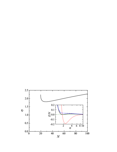
Figure 1: The width of the Gaussian ansatz $\sigma$ as a function of the reduced number of particles $N$ at the $\gamma=1/2$ case. The inset shows the energy per particle predicted by the Gaussian ansatz at the critical number $N_{c}$ (blue dot-dashed line), at the threshold number for metastable states $N_{m}$ (black line), and at the stable configuration $N=100$ (red dashed line).

IV Self-bound quantum droplets in free space

In this section, we consider a self-bound quantum droplet in free space with $\omega_{0}=0$.

IV.1 Critical particle numbers and phase diagram

Let us start from the Gaussian variational approach, which provides a qualitative description of the droplet state. As can be seen from Eq. (10) (Petrov2015, ), the radius of the droplet in free space $R\sim\sigma$ is set by competition among the kinetic energy per particle $\epsilon_{\textrm{kin}}/N\propto 1/\sigma^{2}$, the mean-field energy per particle $\epsilon_{\textrm{MF}}/N\propto-N/\sigma^{3}$, and the beyond-mean-field energy per particle $\epsilon_{\textrm{BMF}}/N\propto(N/\sigma^{3})^{1+\gamma}$. The balance between the latter two energies gives rise to a finite Gaussian width $\sigma\sim N^{{}^{1/3}}$. However, for small number of particles the kinetic energy term quickly becomes dominant and makes the droplet state unstable. Indeed, as shown in the inset of Fig. 1 for the $\gamma=1/2$ case, with decreasing particle number the well-defined global minimum in the total energy curve at large particle number (see, i.e., the red dashed line at $N=100$) turns into a local minimum at a threshold $N_{m}$ ($\sim 24$, the black line), and the local minimum eventually disappears at a slightly smaller critical number $N_{c}$ ($\sim 19$, the blue dot-dashed line). For the particle number at the interval $N\in[N_{c},N_{m}]$, the system is metastable, as the particle may escape to free space (with zero energy) through a finite energy barrier. This metastable regime is typically correlated with an abnormal rapid increase in the Gaussian width $\sigma$ when the particle number decreases, as illustrated in Fig. 1.

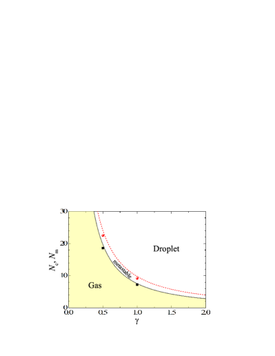
Figure 2: $N_{c}$ and $N_{m}$ as a function of the parameter $\gamma$ predicted by the Gaussian ansatz, which give rise to a phase diagram of the system at a given $\gamma$. The symbols show the results from the extended GPE at $\gamma=1/2$ and $\gamma=1$.

The values of the critical and threshold particle numbers $N_{c}$ and $N_{m}$ could be calculated analytically with the Gaussian ansatz. At $N=N_{c}$, as the local minimum starts to appear, the second derivative of the total energy per particle with respect to $\sigma$ is zero, $\partial^{2}(\epsilon_{\textrm{tot}}/N)/\partial\sigma^{2}=0$. Together with the condition Eq. (11) at $\omega_{0}=0$, we obtain,

$$N_{c}=\frac{2^{3\left(1+\gamma\right)/\left(4\gamma\right)}\left(1+3\gamma\right)^{\left(1+3\gamma\right)/\left(2\gamma\right)}\pi^{3/2}}{3^{3/2}\left(2+\gamma\right)^{3/\left(4\gamma\right)}\left[\gamma\left(1+\gamma\right)\right]^{3/2}}.$$ (31)

On the other hand, at $N=N_{m}$, the disappearance of the local minimum means a zero total energy $\epsilon_{\textrm{tot}}=0$ and we find that,

$$\frac{N_{m}}{N_{c}}=\left(\frac{3}{2}\right)^{3/2}\left(1+\gamma\right)^{1/\left(2\gamma\right)}.$$ (32)

For $\gamma$ increases from $0$ to $\infty$, this ratio increases monotonically from $e^{-1/2}(3/2)^{3/2}\simeq 1.1143$ to $(3/2)^{3/2}\simeq 1.8371$. Moreover, at $\gamma=1/2$ and $\gamma=1$, it takes values $\sqrt{3/2}\simeq 1.2247$ and $3\sqrt{3}/4\simeq 1.2990$, respectively.

In Fig. 2, we show $N_{c}$ and $N_{m}$ as a function of the parameter $\gamma$, which provides a useful phase diagram for the system with a finite particle number. The critical particle numbers obtained by using the Gaussian ansatz (lines) and by solving the stationary extended GPE (symbols) are remarkably close. At $\gamma=1/2$ ($\gamma=1$), we find that the approximate Gaussian predictions $N_{c}\simeq 19.62$ and $N_{m}\simeq 24.03$ ($N_{c}\simeq 7.52$ and $N_{m}\simeq 9.77$) are just a few percent larger than the exact numerical results from the extended GPE $N_{c}\simeq 18.65$ and $N_{m}\simeq 22.55$ (Petrov2015, ) ($N_{c}\simeq 7.23$ and $N_{m}\simeq 9.18$). The critical particle numbers seem to increase significantly with decreasing $\gamma$. This is deceptive, since the unit of the particle number $n_{0}\xi^{3}$ also depends on the parameter $\gamma$. Actually, we find that the actual critical number of particles decreases with decreasing $\gamma$ , if we use the DMC equation of state (Cikojevic2019, ; Cikojevic2020arXiv, ).

Figure 3: The density profiles of a self-bound droplet at $N=N_{c}$ and $N=100N_{c}$, with the parameter $\gamma=1/2$ (a, upper panel) and $\gamma=1$ (b, lower panel). The critical number of particles is obtained by using the variational ansatz. The dashed and dot-dashed lines show the predictions from the Gaussian ansatz and the solid lines show the results of the extended GPE. The density is measured in units of the equilibrium density $n_{0}$.

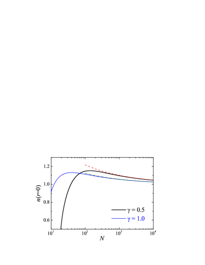
Figure 4: Central density of a self-bound droplet predicted by the extended GPE at the parameter $\gamma=1/2$ (blue thin line) and $\gamma=1$ (black thick line). The dashed and dot-dashed line show the analytic results anticipated at large number of particles, see Eq. (35). The central density is measured in units of the equilibrium density $n_{0}$.

IV.2 Density profile of the droplet

The predictive power of the Gaussian variational approach becomes worse if we consider the density distribution of a droplet. In Fig. 3, we report the density profiles of a self-bound droplet at the critical number of particles $N_{c}$ and $100N_{c}$, calculated by using either the approximate Gaussian ansatz (dashed or dot-dashed lines) or by solving the extend GPE (solid lines). While there is a reasonable agreement between the predictions from the two approaches at the small critical number $N_{c}$, the flat-top structure of the droplet state at the relatively large particle number (i.e., $100N_{c}$) is completely missed by the Gaussian variational approach.

It is readily seen that the density of the flat-top part is larger than unity, which we anticipate in the thermodynamic limit (i.e., $n_{r=0}=[\phi^{(\infty)}]^{2}=1$ in the re-scaled units). This deviation is highlighted in Fig. 4, where we show the central density as a function of the number of particles $N$ at $\gamma=1/2$ and $\gamma=1$. As $N$ increases, the central density initially rises up rapidly, reaches a maximum at about $5N_{c}$ and finally saturates very slowly towards the unity equilibrium density. The slow saturation could be understood from the Laplace’s formula for the surface pressure (i.e., the pressure difference between the droplet and the surrounding vacuum) (FluidMechanicsBook1987, ),

$$P=\frac{2\sigma_{s}}{R},$$ (33)

where $\sigma_{s}=\lim_{\mathcal{S}\rightarrow\infty}[\epsilon_{\textrm{tot}}-\mu^{(\infty)}N]/\mathcal{S}$ is the surface tension, and $R\simeq[3N/(4\pi)]^{1/3}$ and $\mathcal{S}\equiv 4\pi R^{2}$ are the radius and the surface area of the droplet, respectively. In other words, due to the surface tension for a finite-size droplet, the bulk pressure becomes nonzero. By recalling that in the re-scaled units, the bulk pressure is given by

$$P=\left[n\frac{\partial\epsilon}{\partial n}-\epsilon\right]_{n_{r=0}}=-\left(1+\gamma\right)n_{r=0}^{2}\left[1-n_{r=0}^{\gamma}\right],$$ (34)

we find that,

$$n_{r=0}\simeq 1+\frac{2\sigma_{s}}{\gamma\left(1+\gamma\right)}\left(\frac{4\pi}{3}\right)^{1/3}N^{-1/3}.$$ (35)

Following Stringari and Treiner (Stringari1987, ), the surface tension can be written as ($x=r-R$),

$$\sigma_{s} =\intop_{-R}^{\infty}dx\left[\frac{1}{2}\left(\frac{d\phi_{0}}{dx}\right)^{2}+\epsilon\left(\phi_{0},\phi_{0}\right)-\mu^{(\infty)}\phi_{0}^{2}\right],$$ (36)

$$=\frac{1}{\sqrt{2}}\intop_{0}^{1}dn\left[-\left(1+\gamma\right)n+n^{\left(1+\gamma\right)}+\gamma\right]^{1/2},$$ (37)

where in the second line we have used the equation of motion

$$-\frac{1}{2}\left(\frac{d\phi_{0}}{dx}\right)^{2}-\left(1+\gamma\right)\phi_{0}^{4}+\phi_{0}^{4+2\gamma}=\mu^{(\infty)}\phi_{0}^{2}$$ (38)

valid in the thermodynamic limit to convert $dx$ to $dn$, where $n\equiv\phi_{0}^{2}(x)$. It is then straightforward to perform the integration, and we find $\sigma_{s}(\gamma=1/2)=3(1+\sqrt{3})/35\simeq 0.234176$ (Petrov2015, ) and $\sigma_{s}(\gamma=1)=2^{-3/2}\simeq 0.353553$. The surface tension increases with increasing $\gamma$. For sufficiently large $\gamma$, it takes the form,

$$\sigma_{s}\left(\gamma\rightarrow\infty\right)\simeq\frac{\sqrt{2\gamma}}{3}.$$ (39)

In Fig. 4, we show the asymptotic behavior Eq. (35) of the central density by using dashed and dot-dashed lines, for $\gamma=1/2$ and $\gamma=1$, respectively. At large particle number $N>10^{3}$, the asymptotic relation works extremely well.

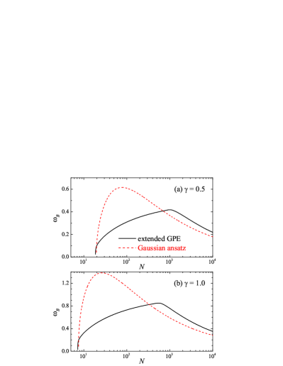
Figure 5: Breathing mode frequency $\omega_{B}$ of a self-bound droplet predicted by the Gaussian ansatz (red dashed lines) and the extended GPE (black solid lines) at the parameters $\gamma=1/2$ (a, upper panel) and $\gamma=1$ (b, low panel).

IV.3 Collective excitations of the droplet

We now turn to consider the collective excitations of a self-bound quantum droplet, starting from the lowest monopole mode, the breathing mode. In Fig. 5, we show breathing mode frequencies as a function of the particle number at $\gamma=1/2$ (a) and $\gamma=1$ (b), predicted by the Gaussian variational approach (dashed line) and by the Bogoliubov equations (solid lines). In sharp contrast to the one-dimensional case, where there is a good agreement between the results from the two methods (Astrakharchik2018, ), here we find that the Gaussian variational approach strongly over-estimates the breathing mode frequency for small number of particles and incorrectly predicts a large peak at $N\sim 4N_{c}$. Only at very large particle number, i.e., $N>50N_{c}$, the variational ansatz begins to provide qualitatively correct mode frequency $\omega_{B}\propto\sqrt{N/\sigma^{5}}\propto 1/R$. This decrease in the breathing mode frequency at large number of particles is anticipated. As we shall discuss later, the breathing mode is the lowest compressional sound mode, whose frequency is given by $\omega_{B}\simeq ck_{B}$, where $c$ is the bulk sound velocity and $k_{B}$ is the characteristic wave-vector of the breathing mode. As $k_{B}$ is inversely proportional to the radius of the droplet, i.e., $k_{B}\propto 1/R$, the breathing mode frequency $\omega_{B}\propto 1/R$ then has to decrease, when the radius of the droplet becomes larger. This leads to a peak in the breathing mode frequency as a function of the number of particles, as shown by the red dashed lines in Fig. 5.

Figure 6: Excitation frequencies $\omega_{ln}$ ($l\leq 9$ and $n\leq 2$) of a self-bound droplet, as a function of the reduced particle number $N$ at the parameter $\gamma=1/2$ (a, upper panel) and $\gamma=1$ (b, lower panel). The red dashed lines show the surface modes $\omega_{l\geq 2,n=0}$ and the blue dot-dashed lines shows the other bulk modes. The black thick lines plot the particle-emission continuum $-\mu$, above which the excitations become unbound and acquire a free-particle dispersion relation.

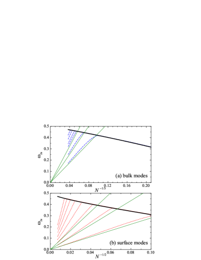
Figure 7: Re-plot of the excitation frequencies $\omega_{ln}$ ($l\leq 9$ and $n\leq 2$) of a self-bound droplet at the parameter $\gamma=1/2$, as a function of $N^{-1/3}$ (a, upper panel with bulk modes only) and $N^{-1/2}$ (b, lower panel with surface modes only). The green straight lines show the analytic results anticipated for a large droplet.

In Fig. 6, we present the whole spectrum of collective excitations $\omega_{ln}$ ($l\leq 9$ and $n\leq 2$) as a function of the particle number $N$ at the parameter $\gamma=1/2$ (a) and $\gamma=1$ (b). Basically, Fig. 6(a) re-plots the mode frequencies found earlier by Petrov (see Fig. 1(b) in Ref. (Petrov2015, )), but with a minor difference. That is, we consider a larger regime for the number of particles, so the mode frequencies $\omega_{ln}$ with nonzero radial quantum numbers $n\neq 0$ start to show up. In the figure, those mode frequencies are plotted by using blue dot-dashed lines, together with the breathing mode frequency $\omega_{00}$. In contrast, the mode frequencies with $l\geq 2$ and $n=0$ are shown by using red dashed lines. The different illustration of the modes comes from their different classification and characters. The former is the so-called bulk mode, which is basically the sound mode spreading throughout the whole droplet; while the latter is referred to as the surface mode that only propagates at the edge of the droplet and uses the surface tension as the restoring force for propagation (FluidMechanicsBook1987, ). These two kinds of modes only survive below the particle-emission threshold, i.e., $\omega_{ln}\leq-\mu$. To understand this, let us recall Eq. (27) and note that the quasi-particle energy $\omega_{ln}$ is measured with respect to the chemical potential $\mu$, instead of the energy of the surrounding vacuum (which is zero). In the frame of the vacuum, the actual energy of the quasi-particle is then $\omega_{ln}+\mu>0$, if the excitation energy $\omega_{ln}$ is above the particle-emission threshold. Therefore, the quasi-particle will tunnel into the vacuum and acquires the free-particle dispersion relation (i.e., the continuum). In other words, the negative chemical potential of the droplet provides an effective confining potential to quasi-particles within the droplet and this leads to the discrete bulk and surface modes below the particle-emission threshold.

Because of their different characters, the frequencies of the bulk and surface modes have distinct dependences on the reduced number of particles. For the bulk modes, if we approximate the droplet as a ball with a sharp edge and radius $R$, we may write

$$\omega_{ln}^{(\textrm{bulk})}\simeq ck_{ln}=c\frac{z_{ln}}{R}\simeq cz_{ln}\left(\frac{4\pi}{3}\right)^{1/3}N^{-1/3},$$ (40)

where in the re-scaled units the speed of sound $c=\sqrt{(\partial P/\partial n)/m}$ is given by

$$c=\sqrt{\gamma\left(1+\gamma\right)}$$ (41)

and $k_{ln}$ is the wave-vector of the mode satisfying the hard-wall boundary condition $j_{l}(k_{ln}R)=0$, where $j_{l}(x)$ is the spherical Bessel function of the first kind with zeros $z_{ln}$. For $l=0$, the zeros are given by $z_{0n}=(n+1)\pi$. For nonzero angular momentum, we have $z_{11}\simeq 4.4934$, $z_{12}\simeq 7.7253$, $\cdots$, $z_{21}\simeq 5.7635$, and so on. On the other hand, the dispersion relation of the surface modes can be obtained by solving a Laplace’s equation for the velocity field with a boundary condition set by Eq. (33), i.e., $\omega_{l0}^{2}=l(l-1)(l+2)\sigma_{s}/(n_{r=0}mR^{3})$ (FluidMechanicsBook1987, ), which in the re-scale units takes the form,

$$\omega_{l0}^{(\textrm{surface})}\simeq\sqrt{\frac{4\pi l\left(l-1\right)\left(l+2\right)\sigma_{s}}{3}}N^{-1/2}.$$ (42)

It is clear that the bulk and surface mode frequencies scale like $N^{-1/3}$ and $N^{-1/2}$, respectively. To highlight those different scaling behaviors, in Fig. 7 we re-plot the mode frequencies as a function of $N^{-1/3}$ and $N^{-1/2}$ in (a) and (b), respectively. The analytic predictions by Eq. (40) and Eq. (42) are also shown by thin green lines for the lowest three modes. We find an excellent agreement between the numerical and analytical results for sufficiently large number of particles. The agreement for the surface modes is particularly satisfactory, presumably due to their lower energy that favors the application of the hydrodynamic equations.

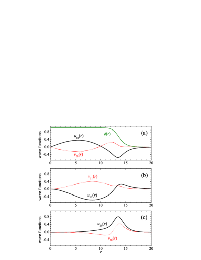
Figure 8: The quasi-particle wave-functions $u_{ln}(r)$ (black solid lines) and $v_{ln}(r)$ (red dashed lines) at a large reduced particle number $N=10000$ and at the parameter $\gamma=1/2$. We show the two lowest non-trivial bulk modes (a, $l=n=0$ and b, $l=n=1$) and the lowest surface mode (c, $l=2$ and $n=0$). In (a), we show also the condensate wave-function $\phi(r)$ of the free-bound droplet. We note that, in (a) the wave-functions of the breathing mode $u_{00}(r)$ and $v_{00}(r)$ have a node in the radial direction, due to our definition of the radial quantum number $n$ (NoteNumberNodes, ).

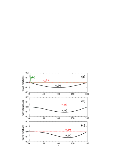
Figure 9: The quasi-particle wave-functions $u_{ln}(r)$ (black solid lines) and $v_{ln}(r)$ (red dashed lines) at a small reduced particle number $N=60$ and at the parameter $\gamma=1/2$. We show the two lowest non-trivial bulk modes (a, $l=n=0$ and b, $l=n=1$) and the lowest surface mode (c, $l=2$ and $n=0$). In (a), we show also the condensate wave-function $\phi(r)$ of the free-bound droplet. We note that, the cut-off length in our numerical calculations is $r_{\textrm{max}}\simeq 200$.

The different characters of the bulk and surface modes might also be understood from the quasi-particle wave-functions $u_{ln}(r)$ and $v_{ln}(r)$, which can be experimentally probed by measuring the density fluctuation $\delta n(r)\sim[u_{ln}(r)+v_{ln}(r)]\phi_{0}(r)$. In Fig. 8, we show $u_{ln}(r)$ and $v_{ln}(r)$ at $\gamma=1/2$ and at a large number of particles $N=10000$, so the bulk mode frequencies $\omega_{00}$ (a) and $\omega_{11}$ (b), and the surface mode frequency $\omega_{20}$ (c) are all below the particle-emission continuum. In comparison with the condensate wave-function $\phi_{0}(r)$, i.e., the green line in Fig. 8(a), it is evident that the wave-functions of the bulk modes fluctuate within the whole droplet, while the wave-functions of the surface modes localize near the edge of the droplet only. Outside the droplet, all the wave-functions decay exponentially. Thus, for the surface modes, the excitations mainly perturb the density in the surface region, as we anticipate.

Interestingly, for small number of particles, there is a threshold $N_{\textrm{th}}$, below which all the excitation modes of a stable droplet in the interval $N_{m}<N<N_{\textrm{th}}$ lie above the particle-emission threshold $-\mu$ (see Fig. 6). For $\gamma=1/2$ and $\gamma=1$, we find that $N_{\textrm{th}}\simeq 94.2$ (Petrov2015, ) and $N_{\textrm{th}}\simeq 36.5$, respectively. As pointed out by Petrov (Petrov2015, ), in such an interval, the droplet fails to create bound excitations and therefore cannot dissipate the energy added to the system. In other words, upon excitations the droplet needs to emit particles and evaporate automatically. This self-evaporation phenomenon has recently been simulated by Ferioli and co-workers, by preparing the droplet slightly out of equilibrium and consequently monitoring the evolution of the droplet size (Ferioli2020, ) (see also the work (Cikojevic2020arXiv, )). The oscillation in the size is found to decay quickly and the breathing mode frequency extracted from the simulations decreases in time until it touches the particle-emission threshold.

In solving the Bogoliubov equations, the self-evaporation mechanism can alternatively be understood from the quasi-particle wave-functions $u_{ln}(r)$ and $v_{ln}(r)$, as shown in Fig. 9, for the number of particles $N=60<N_{\textrm{th}}$ at the parameter $\gamma=1/2$. We find that, for all the bulk and surface modes (considered in the figure), the hole component of the wave-functions $v_{ln}(r)$ disappears, and the particle component $u_{ln}(r)$ becomes unbound, in the sense that the shape of $u_{ln}(r)$ becomes completely irrelevant to the droplet and is set by the maximum cut-off length $r_{\textrm{max}}\simeq 200$ considered in the numerical calculations. This exactly implies the emission of particles upon excitations.

For a general parameter $\gamma$, the threshold number $N_{\textrm{th}}$ might be analytically determined, by tracing the crossing point between the lowest surface mode frequency $\omega_{20}$ and the particle-emission threshold $-\mu$. By using Eq. (42), we find $\omega_{20}=4\sqrt{2\pi\sigma_{s}/(3N)}$. For the chemical potential, we note that, in the re-scaled units the total energy is approximately given by $\epsilon_{\textrm{tot}}/N\simeq-\gamma+\epsilon_{s}N^{-1/3}$, where $\epsilon_{s}=(36\pi)^{1/3}\sigma_{s}$ is the surface energy (Stringari1987, ). Hence, we obtain $\mu=\partial\epsilon_{\textrm{tot}}/\partial N=-\gamma+(32\pi/3)^{1/3}\sigma_{s}N^{-1/3}$. This $N^{-1/3}$-dependence of the chemical potential can also be seen from the particle-emission threshold in Fig. 7(a). By taking $\omega_{20}=-\mu$ at the threshold number of particles, we find that

$$N_{\textrm{th}}\simeq\frac{32\pi\sigma_{s}}{3\left[\gamma-\left(\gamma\sigma_{s}\right)^{2/3}\right]^{2}}.$$ (43)

This analytic expression predicts $N_{\textrm{th}}\simeq 115.5$ and $N_{\textrm{th}}\simeq 47.4$ at $\gamma=1/2$ and $\gamma=1$, respectively, which are about $20-30\%$ larger than the numerical results.

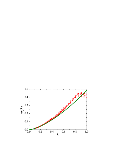
Figure 10: Excitation frequencies of the surface modes $\omega_{l,n=0}$ from $l=2$ to $l=9$, at the parameter $\gamma=1/2$ for some selected reduced particle numbers $N$ ranging from $500$ to $30000$, as a function of the effective wave-vector $k=[l(l-1)(l+2)]^{1/3}/R$. The green thick line shows the anticipated dispersion relation $\omega_{s}(k)=\sqrt{\sigma_{s}}k^{3/2}$, where the dimensionless surface tension $\sigma_{s}=6(1+\sqrt{3})/35\simeq 0.234176$ at the parameter $\gamma=1/2$.

The existence of the surface modes is a unique feature of quantum droplets. By examining more closely Eq. (42), it seems useful to define an effective wave-vector (Chin1995, )

$$k=\frac{\left[l\left(l-1\right)\left(l+2\right)\right]^{1/3}}{R}$$ (44)

and re-cast the dispersion relation into the form,

$$\omega_{s}\left(k\right)=\sqrt{\sigma_{s}}k^{3/2}.$$ (45)

As the discreteness of the excitation spectrum becomes less important for large droplets, we anticipate that such an exotic $k^{3/2}$ dispersion relation should be valid at sufficiently large number of particles. We have calculated the surface mode frequencies with $2\leq l\leq 9$ for a large droplet with $N$ ranging from $500$ to $30000$, and have taken the root-mean-square (rms) radius

$$R=\sqrt{\frac{5}{3}\left\langle r^{2}\right\rangle}$$ (46)

to reduce the finite-size effect. The surface mode frequencies are plotted as a function of the effective wave-vector $k$ in Fig. 10. Indeed, we observe that the data points of the mode frequencies nicely collapse onto the predicted dispersion relation Eq. (45), when the number of particles becomes sufficiently large or the effective wave-vector becomes sufficiently small. At larger effective wave-vector (i.e., $k>0.8$), the curve of the data points turns out to abruptly become flat. This is caused by either a small number of particles or a large angular momentum $l$, at which the surface mode frequency starts to merge with the particle-emission threshold $\left|\mu\right|$, so the mode frequency $\omega_{l0}$ can no longer be described by the ripplon dispersion Eq. (42). Experimentally, the frequency of the quadrupole surface mode $\omega_{20}$ could be readily measured, together with the rms radius $R$ of the droplet, at different large number of particles. As a result, the dispersion relation Eq. (45) might be verified and the surface tension $\sigma_{s}$ is then experimentally determined.

V Quantum droplets in harmonic traps

Let us now turn to consider the external harmonic trapping potential. We will focus on the case with the parameter $\gamma=1/2$.

V.1 $\omega_{0}$-dependence of the droplet profile and collective modes

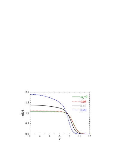
Figure 11: The density profiles of a droplet with and without the harmonic trapping potential at the reduced particle number $N=3000$ and at the parameter $\gamma=1/2$.

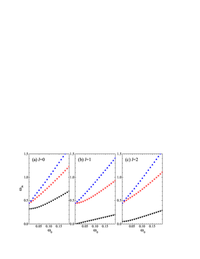
Figure 12: The dependence of excitation frequencies on the external harmonic trapping potential: (a) $l=0$, (b) $l=1$ and (c) $l=2$. In each panel, $n=0$, $n=1$ and $n=2$ from bottom to top. We take the reduced number of particles $N=3000$ the parameter $\gamma=1/2$.

For a droplet with the size $R\simeq[3N/(4\pi)]^{1/3}$, qualitatively we may anticipate the effect of the external trapping potential will become important once the potential energy at the droplet edge $\omega_{0}^{2}R^{2}/2$ becomes comparable with the “binding energy” of the droplet $\left|\mu\right|$ in the absence of the trap, i.e., $\omega_{0}^{2}R^{2}/2\sim\left|\mu^{(\infty)}\right|=\gamma$, which gives rise to a characteristic trapping frequency,

$$\omega_{0,c}\sim\sqrt{2\gamma}\left(\frac{4\pi}{3}\right)^{1/3}N^{-1/3}.$$ (47)

In Fig. 11, we report the density profiles of the droplet with the number of particles $N=3000$ at different trapping frequencies as indicated. In this case, the characteristic trapping frequency $\omega_{0,c}\sim 0.10$. Indeed, we find that the density profiles at $\omega_{0}=0.03\ll\omega_{0,c}$ only differs sightly from the self-bound droplet (at $\omega_{0}=0$). While at the trapping frequency $\omega_{0}=0.20>\omega_{0,c}$, there is a significant modulation to the density distribution due to the trapping potential. The flat-top structure is lost and the central density deviates notably from the equilibrium density in free space, i.e., $n_{r=0}=1$, as we expect for a large self-bound droplet. As we shall discuss in detail in the next section, the choice of a dimensionless trapping frequency $\omega_{0}=0.03$ follows roughly the experiment conditions in Ref. (Semeghini2018, ), where there is a residual trapping frequency $\omega_{z}\sim 2\pi\times 12$ Hz along the axial direction. The negligible trapping effect at $\omega_{0}=0.03$ shown in Fig. 11 therefore strongly supports the claim that a self-bound droplet has been observed in free space (Semeghini2018, ).

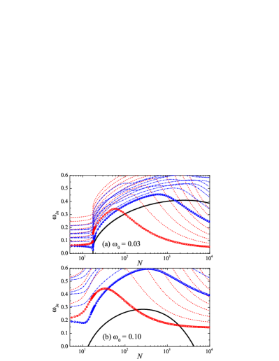
Figure 13: Excitation frequencies $\omega_{ln}$ ($l\leq 9$ and $n\leq 2$) of an ultradilute droplet in harmonic traps, as a function of the reduced particle number $N$ at the dimensionless trapping frequency $\omega_{0}=0.03$ (a, upper panel) and $\omega_{0}=0.10$ (b, lower panel). The red dashed lines show the surface modes $\omega_{l\geq 2,n=0}$ and the blue dot-dashed lines show other bulk modes. The lowest surface mode $\omega_{20}$ (i.e, quadruple mode) and the lowest bulk mode (breathing monopole mode) are emphasized by the red open squares and blue solid circles, respectively. The black thick lines show $-\mu$. Here, we take the parameter $\gamma=1/2$.

In Fig. 12, we show the frequencies $\omega_{ln}$ of the lowest three monopole (a), dipole (b) and quadrupole modes (c) as a function of the trapping frequency $\omega_{0}$, for a droplet with a large number of particles $N=3000$, at which in the self-bound limit ($\omega_{0}\rightarrow 0$) the discrete modes $\omega_{00}$ and $\omega_{20}$ already show up below the particle-emission threshold. The lowest dipole mode is trivial and its mode frequency is always the trapping frequency, $\omega_{10}=\omega_{0}$, owing to the well-known Kohn theorem that under the harmonic trapping potential the center-of-mass motion is an exact excited state of the system. The frequencies of the breathing mode (i.e., the lowest monopole mode) and of the $l=2$ surface mode (i.e., the lowest quadruple mode) clearly show a super-linear dependence on $\omega_{0}$, indicating that those modes are not so sensitive to the small trapping frequency satisfying $\omega_{0}<\omega_{0,c}$. In contrast, for the higher excitation modes (i.e., those with $n=2$), we typically find a linear dependence of the mode frequency on $\omega_{0}$. This somehow suggests that those modes are mainly related to the external trapping potential, instead of the intrinsic properties of the droplet. In fact, in the self-bound limit those modes enter the particle-emission continuum and become uncorrelated with the droplet.

V.2 Excitation spectrum and phase diagram

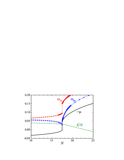
Figure 14: The enlarged view of the breathing and quadruple excitation frequencies in Fig. 13(a), $\omega_{00}$ and $\omega_{20}$, near the critical number of particles. The black thick line shows $-\mu$ and the green dot-dashed line corresponds to the energy per particle $E/N$. There is a first-order quantum phase transition from the droplet state to a gas-like state at $N\simeq 17.5$.

In Fig. 13, we report the whole excitation spectrum $\omega_{ln}$ as a function of the number of particles $N$, at $\omega_{0}=0.03$ (a) and $\omega_{0}=0.10$ (b). We show also the particle-emission threshold $-\mu$ in black thick lines, although it becomes less well-defined in the presence of an external harmonic trap. Following the earlier convention, we have plotted the bulk and surface modes by using blue dot-dashed lines and red dashed lines. Furthermore, the breathing mode and the lowest $l=2$ surface mode are highlighted using blue circles and red squares, respectively. Three features of the figure are worth noting.

First, due to the existence of the external trapping potential, the excitations become all bound and have discrete mode frequency. There is no longer the particle-emission continuum. In particular, the system now can have arbitrarily small number of particles, since the trapping potential plays the role of container to confine particles in the gas-like state. In the limit of vanishing number of particles, $N\rightarrow 0$, the system is basically a non-interacting gas, so the excitation spectrum can be easily understood. For instance, the frequencies of the breathing mode and the $l=2$ surface mode reach the non-interacting value $\omega_{B}=\omega_{Q}=2\omega_{0}$. On the other hand, in the large particle number limit, $N\rightarrow\infty$, the frequency of each mode tend to a finite value. This is particularly clear for the lowest surface mode, whose frequency gradually approaches $\omega_{Q}=\sqrt{2}\omega_{0}$, which is anticipated for interacting quantum gases (Dalfovo1999, ; Hu2004, ).

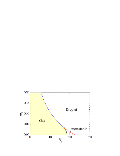
Figure 15: Phase diagram of a harmonically trapped system near the gas-liquid transition at the parameter $\gamma=1/2$. The solid line shows the first-order transition, while the dashed or dot-dashed line indicates a smooth transition. The window for metastable states shrinks with increasing trapping potential and disappears at the dimensionless trapping frequency $\omega_{0}\simeq 0.032$, as indicated by the orange circle.

Second, at small trapping frequency (see Fig. 13(a)), we typically find a jump in all the mode frequencies at a critical number of particles. This is highlighted in Fig. 14, where at $N_{c}\sim 17.5$ we also find a discontinuity in the chemical potential $-\mu$ and a kink in the energy per particle $E/N$ (see the green dot-dashed line). For large trapping frequency, such a jump disappears (see Fig. 13(b)). Instead, we start to observe the formation of a dip structure in the breathing mode frequency. The jump or discontinuity at small trapping frequency is easy to understand. It is simply the first-order transition from the droplet state to the gas-like state that we already discussed in Fig. 2 in the absence of the external harmonic trap. We should also find a metastable state for a small window in the number of particles, if we try different Gaussian ansatz (with different width) as the initial state for solving the stationary GPE and then the Bogoliubov equations. Indeed, as shown in Fig. 15, we can determine the critical and threshold numbers of particles, $N_{c}$ and $N_{m}$, at different trapping potential. Remarkably, the window for the metastable state shrinks with increasing trapping frequency $\omega_{0}$. It closes completely at the tri-critical point $\omega_{0}\sim 0.032$ (see, i.e., the orange circle in Fig. 15). Above this value, the transition from the droplet state to the gas-like phase becomes smooth (i.e., second-order) and we mark the dip position in the breathing mode frequency as the transition point.

Finally, it can be readily seen from Fig. 13 that, although the excitation spectrum changes a lot under the external trapping potential, the qualitative behavior of the surface mode frequencies, as a function of the number of particles, turn out to be very robust. They decrease with increasing number of particles, following the same pattern as in the absence of the external trapping potential (i.e.. compared to Fig. 6(a)). To better understand this, let us now check more carefully the quasi-particle wave-functions of the surface modes.

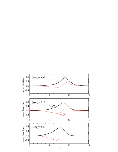
Figure 16: The quasi-particle wave-functions of the lowest surface mode $\omega_{20}$ at three trapping frequencies $\omega_{0}=0.03$ (a), $\omega_{0}=0.10$ (b) and $\omega_{0}=0.20$ (c) and at a large reduced particle number $N=3000$. The solid and dashed lines show $u_{20}(r)$ and $v_{20}(r)$, respectively. Here, we take the parameter $\gamma=1/2$.

V.3 Surface modes

In Fig. 16, we show the wave-functions $u_{20}(r)$ (solid lines) and $v_{20}(r)$ (dashed lines) of the lowest surface mode at $N=3000$ and at three different trapping potentials. We find that the shapes of the wave-functions are qualitatively unchanged with increasing trapping frequency, although there is a slight shift in the peak position in $u_{20}(r)$, This shift is presumably due to the reduced droplet size, since the external trapping potential provides additional confinement to the particles. Indeed, by examining the density profiles in Fig. 11, we observe that the droplet edge shifts from $R\sim 9$ to $R\sim 8.5$, and finally to $R\sim 8$, when we increase the trapping frequency from $\omega_{0}=0.03$ to $\omega_{0}=0.10$, and to $\omega_{0}=0.20$, which is consistent with the peak position found in the wave-functions $u_{20}(r)$.

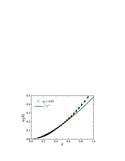
Figure 17: Excitation frequencies of the surface modes $\omega_{l,n=0}$ from $l=2$ to $l=9$, for some selected reduced particle numbers $N$ ranging from $500$ to $30000$, as a function of the effective wave-vector $k=[l(l-1)(l+2)]^{1/3}/R$ at the harmonic trapping potential $\omega_{0}=0.03$ (squares). As the external trapping potential gives rise to a background contribution ($\sim\omega_{0}$) to the mode frequency, we have defined $\omega_{s}\simeq\omega_{l0}-\omega_{0}$. The green thick line shows the anticipated dispersion relation $\omega_{s}(k)=\sqrt{\sigma_{s}}k^{3/2}$, where the dimensionless surface tension $\sigma_{s}=6(1+\sqrt{3})/35\simeq 0.234176$ at the parameter $\gamma=1/2$.

It is now natural to ask, could we experimentally confirm the exotic $k^{3/2}$ dispersion relation for the surface modes under a reasonably small external trapping potential? We consider the strategy adopted earlier and use Eq. (46) to convert the angular momentum $2\leq l\leq 9$ to an effective wave-vector $k$ at different number of particles $N\subseteq(500,30000$). In this interval, we find that the surface mode frequency is typically pushed up by the external trapping potential by an amount $\sim\omega_{0}$. Therefore, we subtract this background contribution and define $\omega_{s}\simeq\omega_{l0}-\omega_{0}$. In Fig. 17, we show $\omega_{s}$ as a function of the effective wave-vector $k$ at a weak trapping frequency $\omega_{0}=0.03$. We observe that, overall the data points roughly follow the expected dispersion relation $\omega_{s}(k)=\sqrt{\sigma_{s}}k^{3/2}$, which is shown by a thick green line. However, we can not find a perfect data collapse at large number of particles as in the self-bound droplet (cf. Fig. 10). The data points become more scattered as we increase the trapping potential to $\omega_{0}=0.20$ (not shown in the figure). Presumably, this is due to the difficulty in determining the radius $R$ of the droplet: when the external trapping frequency increases, the flat-top structure in the density profile ceases to exist and the sharp edge becomes less well-defined. The inaccurate determination of the droplet radius in turn makes the effective wave-vector $k$ ill-defined and hence leads to scattered data points in the dispersion relation. Nevertheless, at the weak external trapping potential considered in Fig. 17, the scattering of the data points is not obvious and the nonlinearity of the dispersion is evident. We may then measure the surface tension from a curve fitting to the anticipated $k^{3/2}$ dispersion relation at small momentum.

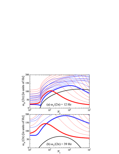
Figure 18: Excitation frequencies $\omega_{ln}$ ($l\leq 9$ and $n\leq 2$) of a ³⁹K binary mixture at the magnetic field $B=56.453$ G, as a function of the actual particle number $N_{a}$ at the trapping frequency $\omega_{T}=2\pi\times 12$ Hz (a, upper panel) and $\omega_{T}=2\pi\times 39$ Hz (b, lower panel). The red dashed lines show the surface modes $\omega_{l\geq 2,n=0}$ and the blue dot-dashed lines shows the other bulk modes. The lowest surface mode $\omega_{20}$ (i.e, quadruple mode) and the lowest bulk mode (breathing monopole mode) are shown by the red open squares and blue solid circles, respectively. The black thick lines show $-\mu_{a}$. Here, the parameter $\gamma=0.373<1/2$ according to the parameterization to the DMC equation of state (Cikojevic2020arXiv, ). We note that, the breathing mode ($\omega_{00}$) and quadrupole mode ($\omega_{20}$) without trapping potential have recently been investigated by Cikojević and co-workers (Cikojevic2020arXiv, ).

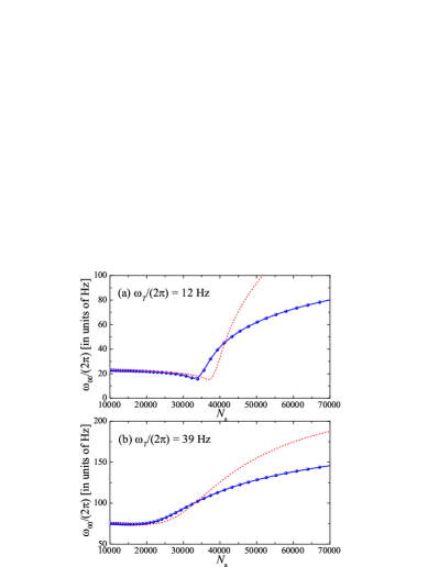
Figure 19: Breathing mode frequencies $\omega_{00}$ of a ³⁹K binary mixture at the magnetic field $B=56.453$ G, as a function of the actual particle number $N_{a}$ near the gas-liquid transition at the trapping frequency $\omega_{T}=2\pi\times 12$ Hz (a, upper panel) and $\omega_{T}=2\pi\times 39$ Hz (b, lower panel). The solid lines with blue circles show the results of the linearized Bogoliubov equations, while the red dashed lines show the predictions from the Gaussian ansatz.

VI Experimental relevances

To make connection with the experiments, let us focus on the binary ³⁹K mixtures (Cabrera2018, ; Semeghini2018, ). In this case, an accurate calculation of the total energy functional $E(n)$ is difficult, since the intra- and inter-species inter-particle interactions both involve a large effective range of interactions. Here, we consider the recent equation of state obtained by DMC and the related parameterization (Cikojevic2020, ; Cikojevic2020arXiv, ). Let us choose a typical magnetic field $B=56.453$ G, at which the parameters in the total energy functional $E(n)=-A_{0}n^{2}+A_{1}n^{2+\gamma}$ are given by (Cikojevic2020arXiv, ),

$$A_{0} = \alpha\frac{\hbar^{2}a_{11}}{2m},$$ (48)

$$A_{1} = \beta\frac{\hbar^{2}a_{11}^{3\gamma+1}}{2m},$$ (49)

with $\alpha=0.423$, $\beta=8.550$, $\gamma=0.373$ and $a_{11}=70.119a_{\textrm{bohr}}\simeq 3.711$ nm. By using Eq. (2) and Eq. (6), it is straightforward to obtain,

$$\frac{\hbar^{2}}{m\xi^{2}} = \frac{1}{2\beta^{\frac{1}{\gamma}}}\left[\frac{\alpha}{\left(1+\gamma\right)}\right]^{\frac{1+\gamma}{\gamma}}\frac{\hbar^{2}}{ma_{11}^{2}}\simeq 2\pi\hbar\times 392\textrm{ Hz},$$ (50)

$$n_{0}\xi^{3} = \sqrt{8}\beta^{\frac{1}{2\gamma}}\left[\frac{\alpha}{\left(1+\gamma\right)}\right]^{\frac{1+3\gamma}{2\gamma}}\simeq 1423.$$ (51)

Therefore, the residual harmonic trapping frequency $\omega_{T}\sim 2\pi\times 12$ Hz in the LENS experiment (Semeghini2018, ) translates into the dimensionless trapping frequency

$$\omega_{0}=\frac{\hbar\omega_{T}}{\hbar^{2}/\left(m\xi^{2}\right)}=\frac{12}{392}\simeq 0.03,$$ (52)

and the maximum actual number of particles $N_{a}\sim 4\times 10^{5}$ would correspond to a reduced number of particles

$$N=\frac{N_{a}}{n_{0}\xi^{3}}=\frac{4\times 10^{5}}{1423}\simeq 281,$$ (53)

which is already large enough to support a discrete surface mode with $l=2$.

In Fig. 18, we show the excitation spectrum of a binary ³⁹K mixture at $B=56.453$ G, as a function of the actual number of particles $N_{a}$, at the two characteristic trapping frequencies $\omega_{T}=2\pi\times 12$ Hz (a) and $\omega_{T}=2\pi\times 39$ Hz (b), which correspond to $\omega_{0}=0.03$ and $\omega_{0}=0.10$, respectively. Experimentally, it would be interesting to confirm the non-monotonic dependence of the $l=2$ surface mode frequency on the number of particles $N_{a}$, as illustrated by the red squares. For the case of a small trapping frequency $\omega_{T}=2\pi\times 12$ Hz in (a), the peak position might be interpreted as $N_{\textrm{th}}$ ($\times n_{0}\xi^{3}$). We may also qualitatively determine the surface tension $\sigma_{s}$ by fitting the surface mode frequency at the large number of particles with Eq. (42), after the background contribution $\sim\omega_{T}$ being subtracted.

To close the section, let us briefly comment on the applicability of the Gaussian variational approach for a three-dimensional quantum droplet under the external trapping potential, which has been used in the previous studies (Cappellaro2018, ; Cappellaro2017, ). As can be seen from Fig. 19, the Gaussian variational approach predicts very accurate breathing mode frequency in the gas-like state. However, it strongly over-estimates the mode frequency in the droplet state. For the description of the gas-droplet transition, it works qualitatively well and over-estimates the critical number of particles by several tens of percent.

VII Conclusions

In summary, we have presented a systematic investigation of collective excitations of a three-dimensional ultradilute Bose droplet, by using a phenomenological low-energy effective theory (Petrov2015, ). Two approaches have been considered: one is the approximate Gaussian variational approach and another is the numerically exact solution of the Bogoliubov equations. An energy density functional $E(n)$ with a general exponent $\gamma$, i.e., $E(n)=-A_{0}n^{2}+A_{1}n^{2+\gamma}$, has been adopted to provide an accurate equation of state for the droplet (Cikojevic2019, ; Cikojevic2020, ). Furthermore, we have considered the effect of a small external harmonic trapping potential, which may be experimentally used to enhance the stability of the system.

We have found that the first-order droplet-to-gas transition and the excitation spectrum can sensitively depend on the parameter $\gamma$. Yet, in the absence of the external trapping potential, the structure of the spectrum is qualitatively unchanged and is universal. It consists of the discrete bulk modes and surface modes, below the particle-emission threshold $-\mu>0$. For sufficiently large number of particles, they assume the well-known dispersion relations $\omega=ck$ and $\omega_{s}=\sqrt{\sigma_{s}}k^{3/2}$, respectively, if we properly define the effective wave-vector $k$.

In the presence of a weak external harmonic trap, we have observed that the droplet-to-gas transition and the excitation spectrum also change significantly. The phase window for the metastable state shrinks quickly with increasing external trapping potential. Above a tri-critical trapping potential (i.e., $\omega_{0}\simeq 0.032$ at $\gamma=1/2$), the droplet-to-gas transition becomes smooth. Despite the significant change in the excitation spectrum due to the external trapping potential, we have found that the qualitative behavior of the surface modes are very robust. We have shown that it is possible to experimentally confirm their exotic $k^{3/2}$ dispersion relation.

We have also calculated the excitation spectrum for a binary ³⁹K mixture at a typical magnetic field, with the help of the accurate equation of state recently obtained from the diffusion Monte Carlo simulations (Cikojevic2020arXiv, ). A non-monotonic dependence of the $l=2$ surface mode frequency on the actual number of particles has been predicted, under realistic trapping potentials. Both the peak structure and the decrease in the surface mode frequency at large number of particles should be observable in the current experimental configuration. We note, however, that experimentally the three-body loss could become severe at large number of particles. In this respect, a heteronuclear ⁴¹K-⁸⁷Rb mixture with much longer lifetime (DErrico2019, ) could be a better candidate to experimentally confirm our predictions on collective excitations. This possibility will be explored in a future study.

- (1) D. S. Petrov, Quantum Mechanical Stabilization of a Collapsing Bose-Bose Mixture, Phys. Rev. Lett. 115, 155302 (2015).
- (2) I. Ferrier-Barbut, H. Kadau, M. Schmitt, M. Wenzel, and T. Pfau, Observation of Quantum Droplets in a Strongly Dipolar Bose Gas, Phys. Rev. Lett. 116, 215301 (2016).
- (3) M. Schmitt, M. Wenzel, F. Böttcher, I. Ferrier-Barbut, and T. Pfau, Self-bound droplets of a dilute magnetic quantum liquid, Nature (London) 539, 259 (2016).
- (4) L. Chomaz, S. Baier, D. Petter, M. J. Mark, F. Wächtler, L. Santos, and F. Ferlaino, Quantum-Fluctuation-Driven Crossover from a Dilute Bose-Einstein Condensate to a Macrodroplet in a Dipolar Quantum Fluid, Phys. Rev. X 6, 041039 (2016).
- (5) C. Cabrera, L. Tanzi, J. Sanz, B. Naylor, P. Thomas, P. Cheiney, and L. Tarruell, Quantum liquid droplets in a mixture of Bose-Einstein condensates, Science 359, 301 (2018).
- (6) P. Cheiney, C. R. Cabrera, J. Sanz, B. Naylor, L. Tanzi, and L. Tarruell, Bright Soliton to Quantum Droplet Transition in a Mixture of Bose-Einstein Condensates, Phys. Rev. Lett. 120, 135301 (2018).
- (7) G. Semeghini, G. Ferioli, L. Masi, C. Mazzinghi, L. Wolswijk, F. Minardi, M. Modugno, G. Modugno, M. Inguscio, and M. Fattori, Self-Bound Quantum Droplets of Atomic Mixtures in Free Space, Phys. Rev. Lett. 120, 235301 (2018).
- (8) G. Ferioli, G. Semeghini, L. Masi, G. Giusti, G. Modugno, M. Inguscio, A. Gallemi, A. Recati, and M. Fattori, Collisions of Self-Bound Quantum Droplets, Phys. Rev. Lett. 122, 090401 (2019).
- (9) L. Tanzi, E. Lucioni, F. Famà, J. Catani, A. Fioretti, C. Gabbanini, R. N. Bisset, L. Santos, and G. Modugno, Observation of a Dipolar Quantum Gas with Metastable Supersolid Properties, Phys. Rev. Lett. 122, 130405 (2019).
- (10) C. D’Errico, A. Burchianti, M. Prevedelli, L. Salasnich, F. Ancilotto, M. Modugno, F. Minardi, and C. Fort, Observation of quantum droplets in a heteronuclear bosonic mixture, Phys. Rev. Research 1, 033155 (2019).
- (11) F. Böttcher, M. Wenzel, J.-N. Schmidt, M. Guo, T. Langen, I. Ferrier-Barbut, T. Pfau, R. Bombín, J. Sánchez-Baena, J. Boronat, and F. Mazzanti, Dilute dipolar quantum droplets beyond the extended Gross-Pitaevskii equation, Phys. Rev. Research 1, 033088 (2019).
- (12) For a recent review, see, for example, F. Böttcher, J.-N. Schmidt, J. Hertkorn, K. S. H. Ng, S. D. Graham, M. Guo, T. Langen, and T. Pfau, New states of matter with fine-tuned interactions: quantum droplets and dipolar supersolids, arXiv:2007.06391 (2020).
- (13) T. D. Lee, K. Huang, and C. N. Yang, Eigenvalues and Eigenfunctions of a Bose System of Hard Spheres and Its Low-Temperature Properties, Phys. Rev. 106, 1135 (1957).
- (14) S. A. Chin and E. Krotscheck, Surface Excitations of Helium Droplets, Phys. Rev. Lett. 74, 1143 (1995).
- (15) F. Dalfovo, S. Giorgini, L. P. Pitaevskii, and S. Stringari, Theory of Bose-Einstein condensation in trapped gases, Rev. Mod. Phys. 71, 463 (1999).
- (16) J. Kinast, S. L. Hemmer, M. E. Gehm, A. Turlapov, and J. E. Thomas, Evidence for Superfluidity in a Resonantly Interacting Fermi Gas, Phys. Rev. Lett. 92, 150402 (2004).
- (17) M. Bartenstein, A. Altmeyer, S. Riedl, S. Jochim, C. Chin, J. Hecker Denschlag, and R. Grimm, Collective Excitations of a Degenerate Gas at the BEC-BCS Crossover, Phys. Rev. Lett. 92, 203201 (2004).
- (18) H. Hu, A. Minguzzi, X.-J. Liu, and M. P. Tosi, Collective Modes and Ballistic Expansion of a Fermi Gas in the BCS-BEC Crossover, Phys. Rev. Lett. 93, 190403 (2004).
- (19) M. Holten, L. Bayha, A. C. Klein, P. A. Murthy, P. M. Preiss, and S. Jochim, Anomalous Breaking of Scale Invariance in a Two-Dimensional Fermi Gas, Phys. Rev. Lett. 121, 120401 (2018).
- (20) T. Peppler, P. Dyke, M. Zamorano, S. Hoinka, and C. J. Vale, Quantum Anomaly and 2D-3D Crossover in Strongly Interacting Fermi Gases, Phys. Rev. Lett. 121, 120402 (2018).
- (21) H. Hu, B. C. Mulkerin, U. Toniolo, L. He, and X.-J. Liu, Reduced Quantum Anomaly in a Quasi-Two-Dimensional Fermi Superfluid: Significance of the Confinement-Induced Effective Range of Interactions, Phys. Rev. Lett. 122, 070401 (2019).
- (22) X. Y. Yin, H. Hu, and X.-J. Liu, Few-Body Perspective of a Quantum Anomaly in Two-Dimensional Fermi Gases, Phys. Rev. Lett. 124, 013401 (2020).
- (23) L. Tanzi, S. M. Roccuzzo, E. Lucioni, F. Famà, A. Fioretti, C. Gabbanini, G. Modugno, A. Recati, and S. Stringari, Supersolid symmetry breaking from compressional oscillations in a dipolar quantum gas, Nature (London) 574, 382 (2019).
- (24) M. Guo, F. Böttcher, J. Hertkorn, J.-N. Schmidt, M. Wenzel, H. P. Büchler, T. Langen, and T. Pfau, The low-energy Goldstone mode in a trapped dipolar supersolid, Nature (London) 574, 386 (2019).
- (25) D. Baillie, R. M. Wilson, R. N. Bisset, and P. B. Blakie, Self-bound dipolar droplet: A localized matter wave in free space, Phys. Rev. A 94, 021602(R) (2016).
- (26) F. Wächtler and L. Santos, Ground-state properties and elementary excitations of quantum droplets in dipolar Bose-Einstein condensates, Phys. Rev. A 94, 043618 (2016).
- (27) D. Baillie, R. M. Wilson, and P. B. Blakie, Collective Excitations of Self-Bound Droplets of a Dipolar Quantum Fluid, Phys. Rev. Lett. 119, 255302 (2017).
- (28) For nonzero angular momentum , the radial quantum number denotes the number of nodes in the radial wavefunctions. However, at zero angular momentum, the nodeless wavefunction is the condensate wave-function and is excluded as a wave-function of Bogoliubov quasi-particles. In the sector, therefore, the number of nodes in the radial wavefunctions is given by . Hence, the breathing mode has a node in its radial wavefunction.
- (29) V. Cikojević, L. Vranješ Markic, G. E. Astrakharchik, and J. Boronat, Universality in ultradilute liquid Bose-Bose mixtures, Phys. Rev. A 99, 023618 (2019).
- (30) V. Cikojević, L. Vranješ Markić, and J. Boronat, Finite-range effects in ultradilute quantum drops, New J. Phys. 22, 053045 (2020).
- (31) V. Cikojević, L. Vranješ Markić, M. Pi, M. Barranco, and J. Boronat, Towards a QMC-based density functional including finite-range effects: Excitation modes of a 39K quantum droplet, Phys. Rev. A 102, 033335 (2020).
- (32) A. Bulgac, Dilute Quantum Droplets, Phys. Rev. Lett. 89, 050402 (2002).
- (33) D. Blume, B. D. Esry, Chris H. Greene, N. N. Klausen, and G. J. Hanna, Formation of Atomic Tritium Clusters and Bose-Einstein Condensates, Phys. Rev. Lett. 89, 163402 (2002).
- (34) P. M. A. Mestrom, V. E. Colussi, T. Secker, G. P. Groeneveld, and S. J. J. M. F. Kokkelmans, van der Waals Universality near a Quantum Tricritical Point, Phys. Rev. Lett. 124, 143401 (2020).
- (35) S. Stringari and J. Treiner, Surface properties of liquid 3He and 4He: A density-functional approach, Phys. Rev. B 36, 8369 (1987).
- (36) G. Ferioli, G. Semeghini, S. Terradas-Briansó, L. Masi, M. Fattori, and M. Modugno, Dynamical formation of quantum droplets in a 39K mixture, Phys. Rev. Research 2, 013269 (2020).
- (37) A. Cappellaro, T. Macrì, and L. Salasnich, Collective modes across the soliton-droplet crossover in binary Bose mixtures, Phys. Rev. A 97, 053623 (2018).
- (38) G. E. Astrakharchik and B. A. Malomed, Dynamics of one-dimensional quantum droplets, Phys. Rev. A 98, 013631 (2018).
- (39) M. Tylutki, G. E. Astrakharchik, B. A. Malomed, and D. S. Petrov, Collective excitations of a one-dimensional quantum droplet, Phys. Rev. A 101, 051601(R) (2020).
- (40) H. Hu and X.-J. Liu, Consistent theory of self-bound quantum droplets with bosonic pairing, arXiv:2005.08581v2 (2020); to appear in Physical Review Letters.
- (41) H. Hu, J. Wang, and X.-J. Liu, Microscopic pairing theory of a binary Bose mixture with interspecies attractions: Bosonic BEC-BCS crossover and ultradilute low-dimensional quantum droplets, Phys. Rev. A 102, 043301 (2020).
- (42) H. Hu and X.-J. Liu, Microscopic derivation of the extended Gross-Pitaevskii equation for quantum droplets in binary Bose mixtures, Phys. Rev. A 102, 043302 (2020).
- (43) A. Cappellaro, T. Macrì, G. F. Bertacco, and L. Salasnich, Equation of state and self-bound droplet in Rabi-coupled Bose mixtures, Sci. Rep. 7, 13358 (2017).
- (44) C. Menotti and S. Stringari, Collective oscillations of a one-dimensional trapped Bose-Einstein gas, Phys. Rev. A 66, 043610 (2002).
- (45) H. Hu, G. Xianlong, and X.-J. Liu, Collective modes of a one-dimensional trapped atomic Bose gas at finite temperatures, Phys. Rev. A 90, 013622 (2014).
- (46) H. Pu and N. P. Bigelow, Properties of Two-Species Bose Condensates, Phys. Rev. Lett. 80, 1130 (1998).
- (47) D. A. W. Hutchinson, E. Zaremba, and A. Griffin, Finite Temperature Excitations of a Trapped Bose Gas, Phys. Rev. Lett. 78, 1842 (1997).
- (48) L. D. Landau and E. M. Lifshitz, Fluid Mechanics (Pergamon Press, Oxford, 1987), and .