Symmetry breaking in a two-component system with repulsive interactions and linear coupling

Abstract

We extend the well-known theoretical treatment of the spontaneous symmetry breaking (SSB) in two-component systems combining linear coupling and self-attractive nonlinearity to a system in which the linear coupling competes with repulsive interactions. First, we address one- and two-dimensional (1D and 2D) ground-state (GS) solutions and 2D vortex states with topological charges $S=1$ and $2$, maintained by a confining harmonic-oscillator (HO) potential. The system can be implemented in BEC and optics. By means of the Thomas-Fermi approximation and numerical solution of the underlying coupled Gross-Pitaevskii equations, we demonstrate that SSB takes place, in the GSs and vortices alike, when the cross-component repulsion is stronger that the self-repulsion in each component. The SSB transition is categorized as a supercritical bifurcation, which gives rise to states featuring broken symmetry in an inner area, and intact symmetry in a surrounding layer. Unlike stable GSs and vortices with $S=1$, the states with $S=2$ are unstable against splitting. We also address SSB for 1D gap solitons in the system including a lattice potential. In this case, SSB takes place under the opposite condition, i.e., the cross-component repulsion must be weaker than the self-repulsion, and SSB is exhibited by antisymmetric solitons.

1 Introduction and the model

Spontaneous symmetry breaking (SSB) is a broad class of effects occurring in systems combining spatial or inter-component symmetry and intrinsic nonlinearity [1]. While in linear systems the ground state (GS) exactly reproduces the underlying symmetry [2], and the GS is always a single (non-degenerate) state, self-attraction in binary systems drives a phase transition which destabilizes the symmetric GS, replacing it by a pair of asymmetric ones that are mirror images of each other (so as to maintain the overall symmetry). The transition takes place when the nonlinearity strength attains a certain critical value. Starting from early works [3, 4], many realizations of the SSB phenomenology have been supplied by nonlinear optics and studies of Bose-Einstein condensates (BECs). The similarity of these areas is underlain by the fact that the nonlinear Schrödinger equations [5] and Gross-Pitaevskii equations (GPEs) [6, 7]), which are basic models for optics and BEC, respectively, are essentially identical, with the difference that the evolution variable is the propagation distance, $z$, in optical waveguides, and time, $t$, in BEC. In both cases SSB effects have been predicted in two-components systems, with linear coupling between the components and self-attraction in each component. In optics, a natural realization of the nonlinear couplers and SSB phenomenology in them is offered, in terms of the temporal-domain propagation, by dual-core optical fibers. This setting was studied in detail theoretically [8]-[21] (see also review [22]), and nonlinear switching in the couplers was demonstrated experimentally [23, 24]. The same model may be realized in the spatial domain, considering a planar dual-core nonlinear waveguide [25, 15, 26]. Another class of nonlinear-optical symmetric systems and SSB dynamics in them, which were explored both theoretically and experimentally, is provided by dual-cavity lasers [27]-[30].

A similar BEC system may be realized by loading the condensate into a pair of parallel tunnel-coupled elongated traps, filled by self-attractive BEC and linearly coupled by tunneling of atoms [31]-[33]. SSB effects, chiefly for matter-wave solitons, have been predicted in such dual traps.

A more general two-component system includes, in addition to the self-interaction of each component and linear mixing between them, nonlinear cross-component interaction [34, 35]. In optics, this model applies to the propagation of electromagnetic waves with orthogonal circular polarizations in the fiber with linear-polarization birefringence (that may be induced by ellipticity of the fiber’s cross section), which induces the linear mixing [36]. In BEC, the realization is possible in a single elongated trap filled by a mixture of two different atomic states in the condensate, while the linear (Rabi) mixing is imposed by a radiofrequency field which resonantly couples the states [37]-[41].

A majority of the above-mentioned works addressed effectively one-dimensional (1D) settings. In optics, 2D two-component spatiotemporal propagation may be realized in planar dual-core waveguides [42], and similar realizations were considered for BEC loaded in dual-core “pancake-shaped” traps [43, 44, 45]. The more general system, which includes the inter-component nonlinearity, can be naturally implemented as the spatial-domain propagation in bulk optical waveguides, with the linear mixing of orthogonal circular polarizations induced by intrinsic anisotropy (linear birefringence) in the transverse plane. In BEC, an implementation is offered by a pancake trap filled by a binary condensate, with the radiofrequency-induced coupling between two atomic states.

As said above, the SSB of GSs in previous works was driven by attractive nonlinearity. Self-repulsion does not break the GS symmetry, but it may drive spontaneous breaking of antisymmetry of the first excited state, an example being an antisymmetric bound state of matter-wave gap solitons in tunnel-coupled traps equipped with periodic potentials [46, 43, 32]. The objective of the present work is to demonstrate that, nevertheless, the symmetry of the GS in 1D and 2D linearly-coupled systems with repulsive nonlinearity may be spontaneously broken, replacing it by a pair of asymmetric GSs, provided that the inter-component repulsion dominates over the intra-component nonlinearity, and the GS is made localized by a confining potential. This mechanism is similar to other effects in which the dominant repulsion between two interacting fields (in the absence of the linear coupling between them) makes their uniformly mixed state unstable, well-known examples being phase separation in binary mixtures [49] and the modulational instability in bimodal systems in which the cross-repulsion is stronger than self-repulsion [50].

In terms of BEC, the system is represented by coupled GPEs for wave functions $\phi_{1,2}$ of the two components, written in the 2D form, which includes the confining harmonic-oscillator (HO) potential with strength $\Omega^{2}$, acting in the $\left(x,y\right)$ plane, and scaled atomic mass $m$:

$$i\frac{\partial\phi_{1}}{\partial t}=-\frac{1}{2m}\nabla^{2}\phi_{1}+(g|\phi_{1}|^{2}+\gamma|\phi_{2}|^{2})\phi_{1}+\frac{\Omega^{2}}{2}\left(x^{2}+y^{2}\right)\phi_{1}-\epsilon\phi_{2}$$ (1)

$$i\frac{\partial\phi_{2}}{\partial t}=-\frac{1}{2m}\nabla^{2}\phi_{1}+(g|\phi_{2}|^{2}+\gamma|\phi_{1}|^{2})\phi_{2}+\frac{\Omega^{2}}{2}\left(x^{2}+y^{2}\right)\phi_{2}-\epsilon\phi_{1}.$$ (2)

Here, $\epsilon$ is the coefficient of the linear coupling, while $\gamma>0$ and $g>0$ account for, severally, the cross-repulsion and self-repulsion. These coefficients are subject to the above-mentioned condition of the dominant cross-interaction, $\gamma>g$, except for Section IV (the case of $g<0$, i.e., self-attractive nonlinearity, may be considered too, although it is less interesting than the case of the competition between the cross- and self-repulsion). By means of obvious rescaling of $t$, coordinates, and wave functions we fix

$$g=\Omega^{2}=\epsilon=1,$$ (3)

while $m$ and $\gamma$ are kept as free parameters (a different normalization, with $\epsilon\neq 1$, is adopted below in Section IV, where a different potential is considered).

Equations (1) and (2) conserve the total norm,

$$N=\int\int\left(\left|\phi_{1}\right|^{2}+\left|\phi_{2}\right|^{2}\right)dxdy,$$ (4)

Hamiltonian,

$$H = \int\int\left[\frac{1}{2m}\left(\left|\nabla\phi_{1}\right|^{2}+\left|\nabla\phi_{2}\right|^{2}\right)+\frac{1}{2}\left(\left|\phi_{1}\right|^{4}+\left|\phi_{2}\right|^{4}\right)+\gamma\left|\phi_{1}\right|^{2}\left|\phi_{2}\right|^{2}\right.$$ (5)

$$\left.+\frac{1}{2}\left(x^{2}+y^{2}\right)\left(\left|\phi_{1}\right|^{2}+\left|\phi_{2}\right|^{2}-\left(\phi_{1}\phi_{2}^{\ast}+\phi_{1}^{\ast}\phi_{2}\right)\right)\right]dxdy,$$

where normalization (3) is taken into regard, and $\ast$ stands for the complex conjugate, as well as the total angular momentum,

$$M=i\sum_{j=1,2}\int\int\phi_{j}^{\ast}\left(y\frac{\partial}{\partial x}-x\frac{\partial}{\partial y}\right)\phi_{j}dxdy.$$ (6)

In terms of optics, Eqs. (1) and (2) with $t$ replaced by $z$ and $m$ replaced by the Fresnel number provide a model of the spatial-domain copropagation of waves with orthogonal circular polarizations in a bulk waveguide made of a self-defocusing material, provided that relation $g=\gamma/2$ is imposed, which corresponds to the copropagation of orthogonal circular polarizations. In that case, the HO potential represents the transverse waveguiding structure, and the linear-coupling terms represent linear mixing induced by anisotropy (linear birefringence) of the material.

In Section II, we address the SSB effects in the GS produced by the full 2D version of Eqs. 1), (2) and their 1D reduction, under the above-mentioned condition $\gamma>g$. The relevant solutions are obtained in an analytical form by means of the Thomas-Fermi approximation (TFA), and confirmed by full numerical solutions. Section III addresses vortex states, with topological charges $S=1$ and $2$, in the 2D system, in which SSB is again considered by means of TFA and a full numerical solution. In Section IV we address the symmetry breaking of two-component gap solitons in the 1D system, which is described by Eqs. (1) and (2) with the HO potential replaced by the spatially periodic one, see Eqs. (38) and (39) below. In that case, the situation is drastically different, as SSB takes place in antisymmetric two-component solitons, under the condition opposite to the one mentioned above, i.e., $\gamma<g$, which means that the cross-repulsion is weaker than the intrinsic self-repulsion The paper is concluded by Section V.

2 Spontaneous symmetry breaking (SSB) of the ground states (GSs)

Eigenstates of the system based on Eqs. (1), (2), and (3), with chemical potential $\mu>0$, are looked for as

$$\phi_{1,2}\left(x,y\right)=\exp\left(-i\mu t\right)\varphi_{1,2}(x,y),$$ (7)

where functions $\varphi_{1,2}\left(x,y\right)$ satisfy stationary equations

$$\mu\varphi_{1}=-\frac{1}{2m}\nabla^{2}\varphi_{1}+|\varphi_{1}|^{2}\varphi_{1}+\gamma\left|\varphi_{2}\right|^{2}\varphi_{1}+\frac{1}{2}\left(x^{2}+y^{2}\right)\varphi_{1}-\varphi_{2},$$ (8)

$$\mu\varphi_{2}=-\frac{1}{2m}\nabla^{2}\varphi_{2}+|\varphi_{2}|^{2}\varphi_{2}+\gamma\left|\varphi_{1}\right|^{2}\varphi_{2}+\frac{1}{2}\left(x^{2}+y^{2}\right)\varphi_{2}-\varphi_{1}.$$ (9)

The degree of asymmetry of solutions produced by Eqs. (8) and (9) is quantified by parameter

$$R=\frac{2}{N}\int\int|\varphi_{1}\left(x,y\right)|^{2}dxdy-1,$$ (10)

where $N$ is the total norm defined as per Eq. (4). Obviously, $R=0$ in the case when norms of both components are equal.

In the 1D case, $\nabla^{2}$ is replaced by $\partial^{2}/\partial x^{2}$, $y^{2}$ is dropped in the HO potential, and functions $\varphi_{1,2}(x)$ are always real. In this case, the asymmetry is defined by the 1D version of Eq. (10), definitions of $N$ and $H$, given by Eqs. (4) and (5) are also replaced by their 1D versions, while the definition of the angular momentum [see Eq. (6)] is irrelevant.

2.1 The Thomas-Fermi approximation (TFA)

First, we apply the TFA to Eqs. (8) and (9), dropping, as usual, the derivatives in these equations [6, 7] (which is, formally, tantamount to taking $m\rightarrow\infty$):

$$\mu\varphi_{1}=g\varphi_{1}^{3}+\gamma\varphi_{2}^{2}\varphi_{1}+\frac{1}{2}\left(x^{2}+y^{2}\right)\varphi_{1}-\varphi_{2},$$ (11)

$$\mu\varphi_{2}=g\varphi_{2}^{3}+\gamma\varphi_{1}^{2}\varphi_{2}+\frac{1}{2}\left(x^{2}+y^{2}\right)\varphi_{2}-\varphi_{1}.$$ (12)

Equations (11) and (12) admit two nonzero solutions: an obvious symmetric one,

$$\varphi_{1}^{2}(x,y)=\varphi_{2}^{2}(x,y)=\frac{2\left(\mu+1\right)-\left(x^{2}+y^{2}\right)}{2\left(\gamma+1\right)},$$ (13)

which exists at

$$\frac{1}{2}\left(x^{2}+y^{2}\right)<\mu+1,$$ (14)

and a symmetry-broken (alias asymmetric) solution, which exists under the condition adopted above, $\gamma>1$ (the cross-repulsion is stronger than self-repulsion):

$$\varphi_{1}^{2}+\varphi_{2}^{2}=\mu-\frac{1}{2}\left(x^{2}+y^{2}\right),~{}\varphi_{1}\varphi_{2}=\frac{1}{\gamma-1}.$$ (15)

Formally, solution (15) exists at $\gamma<1$ too, but, having $\varphi_{1}\varphi_{2}<0$, it will make the last (linear-coupling) term in Hamiltonian (5) positive, which definitely implies instability of the respective states [22].

The asymmetric solution given by Eq. (15) exists in a region where it complies with obvious condition $\varphi_{1}^{2}+\varphi_{2}^{2}>2\varphi_{1}\varphi_{2}$, i.e.,

$$x^{2}+y^{2}<2\left(\mu-\frac{2}{\gamma-1}\right).$$ (16)

Note that condition (16) may hold if, at least, it is valid at $x=y=0$, thus a condition necessary for the existence of the asymmetric solution is

$$\mu>\mu^{\mathrm{(cr)}}\equiv\frac{2}{\gamma-1}.$$ (17)

Thus, TFA produces the state with the spontaneously broken symmetry which features a two-layer structure:

$$\left\{\begin{array}[]{c}\mathrm{asymmetric,~{}given~{}by~{}Eq.(\ref{asymm}),~{}in~{}the~{}}inner~{}(central)~{}layer\mathrm{,}{}\\ 0\leq x^{2}+y^{2}<2\left(\mu-2\left(\gamma-1\right)^{-1}\right);\\ \mathrm{symmetric,~{}given~{}by~{}Eq.(\ref{symm}),~{}in~{}the~{}}outer~{}(surrounding)~{}layer\mathrm{,}{}\\ 2\left(\mu-2\left(\gamma-1\right)^{-1}\right)\leq x^{2}+y^{2}<2\left(\mu+1\right)\equiv r_{\mathrm{outer}}^{2};\mathrm{~{}}\end{array}\right.$$ (18)

and zero outside of both layers, i.e., at $x^{2}+y^{2}>r_{\mathrm{outer}}^{2}$. Of course, the exact solution has a small nonzero “tail” in the latter area, which is, as usual, ignored by TFA. Another difference of a numerically exact solution is that the symmetry is slightly broken in the TFA-symmetric layer.

If condition (17) does not hold, the inner layer does not exist, and the entire TFA solution keeps the symmetric form, as given by Eqs. (13) and (14). Its total norm, defined as per Eq. (4) or its 1D version, is

$$\left(N_{\mathrm{TFA}}^{\mathrm{(symm)}}\right)_{\mathrm{2D}} = 2\pi\frac{\left(\mu+1\right)^{2}}{\gamma+1},$$ (19)

$$\left(N_{\mathrm{TFA}}^{\mathrm{(symm)}}\right)_{\mathrm{1D}} = \frac{2^{7/2}}{3}\frac{\left(\mu+1\right)^{3/2}}{\gamma+1},$$ (20)

With the increase of the cross-repulsion strength, $\gamma$, at a fixed norm, the SSB sets in when $\mu$, expressed in terms of the norm of the symmetric GS by means of Eq. (20) or (19), attains critical value (17). After a simple algebra, this condition leads to equations which predict, in the framework of TFA, the critical value of $\gamma$, above which SSB takes place for given $N$,

$$\frac{3N}{2^{7/2}}=\frac{\sqrt{\gamma_{\mathrm{1D}}^{\mathrm{(cr)}}+1}}{\left(\gamma_{\mathrm{1D}}^{\mathrm{(cr)}}-1\right)^{3/2}},$$ (21)

$$\frac{N}{2\pi}=\frac{\gamma_{\mathrm{2D}}^{\mathrm{(cr)}}+1}{\left(\gamma_{\mathrm{2D}}^{\mathrm{(cr)}}-1\right)^{2}}.$$ (22)

In particular, for $N$ large enough, when TFA is a natural approximation, Eqs. (21) and (22) yield critical values of $\gamma$ close to $g\equiv 1$, viz., $\gamma_{\mathrm{1D}}^{\mathrm{(cr)}}\approx 1+\left(16/3N\right)^{2/3}$, $\gamma_{\mathrm{2D}}^{\mathrm{(cr)}}\approx 1+2\sqrt{\pi/N}$.

2.2 Numerical results for 1D states

Numerical solutions for the 1D version of Eqs. (1), (2) and (8), (9) are presented here for the total norm $N=10$, as defined by the 1D form of Eq. (4), since this value makes it possible to produce generic results. Figure 1(a) displays profiles of components $\varphi_{1,2}(x)\equiv\left|\phi_{1,2}(x)\right|$ of the GS, obtained by means of the imaginary-time evolution method [51, 52] applied to Eqs. (1), (2), for $\gamma=2.5$ and $m=1$. Further, Fig. 1(b) produces TFA profiles for the same parameters, constructed as per Eqs. (13), (15), and (18), and provides explicit comparison of this approximate analytical solution for $\varphi_{1}(x)$ with its numerically found counterpart [the comparison for component $\varphi_{2}(x)$ is provided by the juxtaposition of panels (a) and (b) in Fig. 1].

Figure 1(c) summarizes the numerical and analytical results by plotting the asymmetry degree $R$, defined as per Eq. (10), vs. the cross-repulsion strength, $\gamma$, at a fixed value of the norm, $N=10$, and fixed mass, $m=1$, as obtained from the numerical solution, and from TFA, i.e., as produced by the integration of expressions (13), (15), and (18). It is seen that SSB takes place at $\gamma>\gamma_{\mathrm{numer}}^{\mathrm{(cr)}}\approx 1.83$, while its TFA counterpart, obtained from Eq. (21), is $\gamma_{\mathrm{TFA}}^{\mathrm{(cr)}}\approx 1.73$ for $N=10$. The analytically predicted curve $R(\gamma)$ is reasonably close to its numerical counterpart, both showing the SSB transition which may be identified as a supercritical bifurcation [53].

Overall, TFA provides reasonable accuracy for $m=1$, even if, formally speaking, this approximation applies for small values of coefficient $1/(2m)$ in Eqs. (8) and (9). To focus on the role of this parameter, Fig. 2 displays $R$ vs. $1/(2m)$ at $\gamma=2.5$. The SSB disappears at $1/(2m)>2.8$. Another essential characteristic of the GS solutions is the critical value of $\gamma$, above which SSB sets in; recall that, in the framework of TFA, it is predicted by Eq. (21). A set of curves of $\gamma_{\mathrm{1D}}^{\mathrm{(cr)}}(N)$ for several fixed values of the inverse-mass parameter, viz., $1/\left(2m\right)=2$, $0.5$, and $0.05$, are plotted in Fig. 2(b), along with the corresponding TFA limit, corresponding to $1/\left(2m\right)=0$.

The SSB effect corresponding to the supercritical bifurcation implies that, when symmetric and symmetry-broken stationary solutions coexist as stationary ones, the symmetric solution should be unstable. This expectation is corroborated in Fig. 3(a), which shows the time evolution of the maximum values of $|\phi_{1}(x)|$ and $|\phi_{2}(x)|$, produced by direct simulations of coupled equations (1) and (2), for $\gamma=2.5$, $m=1$, and $N=10$. The input is a symmetric solution, with $\varphi_{1}(x)=\varphi_{2}(x)$, and a small perturbation added to it. It is unstable, clearly tending to spontaneously transform into a broken-symmetry state. On the other hand, Fig. 3(b) demonstrates stability of the asymmetric GS for the same values of the parameters.

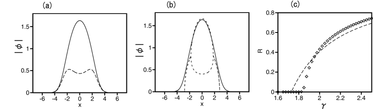
Figure 1: (a) Profiles of components $\left|\phi_{1}(x)\right|$ ans $\left|\phi_{2}(x)\right|$ (solid and dashed lines) in the stable 1D ground state (GS) with broken symmetry between the components. The solution was obtained by means of the imaginary-time-evolution method, applied to the 1D version of Eqs. (1) and (2) with $\gamma=2.5$ and $m=1$, for the total norm $N=10$ [see Eq. (4)]. (b) Comparison of $\left|\phi_{1}(x)\right|$ (the solid line) taken from the same numerical solution, and its TFA counterpart, produced by Eqs. (13), (15), and (18) (the dashed line running close to the solid one); the TFA-produced component $\left|\phi_{2}(x)\right|$ is shown too, by the double-peaked dashed curve. (c) The asymmetry measure, defined as per Eq. (10), vs. $\gamma$, for fixed $m=10$ and $N=10$. The chain of rhombuses and the dashed line show, severally, the numerical results and their TFA-produced counterparts.

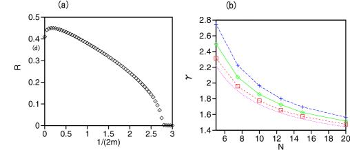
Figure 2: (a) The numerically found asymmetry measure $R$ for the 1D GS solutions [see Eq. (10)], as a function of the inverse-mass parameter, $1/(2m)$. (b) The critical values of $\gamma$, above which the GS symmetry is broken in 1D, as a function of $N$ for fixed values of the inverse-mass coefficient, $1/(2m)=2$ (pluses), $0.5$ (rhombuses), and $0.05$ (squares). The dotted curve is the analytical result predicted by TFA, as per Eq. (21).

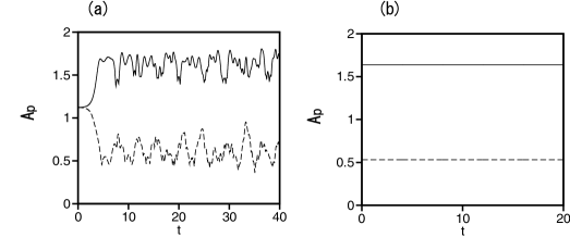
Figure 3: The evolution of the largest values of $|\phi_{1}(x)|$ and $\left|\phi_{2}(x)\right|$ (solid and dashed lines), produced by direct simulations of the 1D version of Eqs. (1) and (2) for $\gamma=2.5$, $m=1$, and total norm $N=10$, starting from (a) the unstable symmetrical state and (b) the stable GS with broken symmetry.

3 Symmetry-breaking 2D vortex states

3.1 The Thomas-Fermi approximation (TFA)

Solutions of the system of coupled 2D equations (1) and (2) with embedded angular momentum are looked for, in the polar coordinates $\left(r,\theta\right)$, as

$$\phi_{1,2}=\exp\left(-i\mu t+iS\theta\right)\varphi_{1,2}(r),$$ (23)

where $\varphi_{1,2}(r)$ are real radial wave functions, and $S=1,2,3,...$ is the integer vorticity, $S=0$ corresponding to the 2D GS. For stationary states represented by ansatz (23), the angular momentum, defined as per Eq. (6), is related to the total norm, $M=SN$.

In the framework of TFA (which was previously applied to delocalized vortex states [54]), the substitution of ansatz (23) leads to the following radial equations, instead of 1D equations (11) and (12):

$$\mu\varphi_{1}=g\varphi_{1}^{3}+\gamma\varphi_{2}^{2}\varphi_{1}+\frac{1}{2}\left(r^{2}+\frac{S^{2}}{r^{2}}\right)\varphi_{1}-\varphi_{2},$$ (24)

$$\mu\varphi_{2}=g\varphi_{2}^{3}+\gamma\varphi_{1}^{2}\varphi_{2}+\frac{1}{2}\left(r^{2}+\frac{S^{2}}{r^{2}}\right)\varphi_{2}-\varphi_{1}.$$ (25)

Straightforward consideration of Eqs. (24) and (25) demonstrates that solutions are different from zero in annulus

$$r_{\mathrm{core}}^{2}<r^{2}<r_{\mathrm{outer}}^{2},$$ (26)

$$r_{\mathrm{outer,core}}^{2}=\mu+1\pm\sqrt{\left(\mu+1\right)^{2}-S^{2}},$$ (27)

provided that $\mu+1>S$. Note that the central “empty” core, in which the TFA solution is zero, is absent in the GS solution (with $S=0$), as Eq. (27) yields $r_{\mathrm{core}}^{2}\left(S=0\right)=0$. In the same case, Eq. (27) yields $r_{\mathrm{outer}}^{2}\left(S=0\right)=2\left(\mu+1\right)$, which coincides with $r_{\mathrm{outer}}^{2}$ given above by Eq. (18) for the GS.

In annulus (26), the symmetric solution of Eqs. (24) and (25) is

$$\varphi_{1,2}^{2}(r)\equiv\varphi^{2}(r)=\frac{\mu+1}{\gamma+1}-\frac{1}{2\left(\gamma+1\right)}\left(r^{2}+\frac{S^{2}}{r^{2}}\right).$$ (28)

Note that setting $S=0$ makes this solution identical to its GS counterpart given by Eq. (13). The total norm of symmetric expression (28) is

$$N_{\mathrm{TFA}}^{\mathrm{(symm)}}(S)=2\pi\frac{\mu+1}{\gamma+1}\sqrt{\left(\mu+1\right)^{2}-S^{2}}$$

$$-\frac{2\pi S^{2}}{\gamma+1}\ln\left(\frac{\mu+1+\sqrt{\left(\mu+1\right)^{2}-S^{2}}}{S}\right),$$ (29)

which, for $S=0$ (the GS), is tantamount to Eq. (19).

Points at which the broken-symmetry solution with $S\geq 1$ (if any) branches off from the symmetric one, given by Eq. (28), are determined by taking the difference of Eqs. (24) and (25), linearizing it for $\varphi_{1}-\varphi_{2}\rightarrow 0$, and cancelling the common infinitesimal factor $\left(\varphi_{1}-\varphi_{2}\right)$:

$$\mu-1=\left(3-\gamma\right)\varphi^{2}(r)+\frac{1}{2}\left(r^{2}+\frac{S^{2}}{r^{2}}\right).$$ (30)

The substitution of the symmetric TFA solution (28) in Eq. (30) leads to the conclusion that the asymmetric solution may exist between the following branching points:

$$r_{\max,\min}^{2}=\mu-\frac{2}{\gamma-1}\pm\sqrt{\left(\mu-\frac{2}{\gamma-1}\right)^{2}-S^{2}}$$ (31)

Thus, TFA predicts the vortex solution with a three-layer structure. First, it vanishes in the empty core and in the peripheral zone,

$$\varphi_{1,2}\left(r<r_{\mathrm{core}}\right)=\varphi_{1,2}\left(r>r_{\mathrm{outer}}\right)=0.$$ (32)

The symmetric solution, as given by Eq. (28), is supported in two edge layers,

$$r_{\mathrm{core}}^{2} < r^{2}<r_{\min}^{2},$$ (33)

$$r_{\max}^{2} < r^{2}<r_{\mathrm{outer}}^{2}~{},$$ (34)

with the edges determined by Eqs. (27) and (31). Finally, the broken symmetry is featured by the TFA solution in the inner layer,

$$r_{\min}^{2}<r^{2}<r_{\max}^{2}.$$ (35)

In the framework of TFA, the condition necessary for the existence of the asymmetric solution amount to the existence of real values (31), i.e.,

$$\mu>\mu^{\mathrm{(cr)}}(S)\equiv\frac{2}{\gamma-g}+S,$$ (36)

cf. Eq. (17) for the GS. Further, combining Eq. (36) with expression (29) for the norm of the symmetric vortex state, one can derive an equation for the critical strength of the cross-repulsion, above which the symmetry of the vortex states is broken, cf. Eq. (22) for the 2D GS ($S=0$). In particular, for $S=1$ the equation is

$$N=\frac{2\pi\gamma_{S=1}^{\mathrm{(cr)}}}{\left(\gamma_{S=1}^{\mathrm{(cr)}}-1\right)^{2}}\sqrt{\frac{3\gamma_{S=1}^{\mathrm{(cr)}}-1}{\gamma_{S=1}^{\mathrm{(cr)}}+1}}$$

$$-\frac{2\pi}{\gamma_{S=1}^{\mathrm{(cr)}}+1}\ln\left(\frac{2\gamma_{S=1}^{\mathrm{(cr)}}+\sqrt{\left(\gamma_{S=1}^{\mathrm{(cr)}}+1\right)\left(3\gamma_{S=1}^{\mathrm{(cr)}}-1\right)}}{\gamma_{S=1}^{\mathrm{(cr)}}-1}\right).$$ (37)

3.2 Numerical results for 2D ground and vortex states

Proceeding to numerical results for the 2D system, in Fig. 4(a) we, first, display numerically found radial profiles, $\varphi_{1,2}(r)\equiv\left|\phi_{1,2}(r)\right|$, of the two components of the 2D GS (with $S=0$), for $\gamma=2.3$, $m=1$, and the total 2D norm $N=100$. The numerical profiles are compared to their TFA-predicted counterparts, obtained from Eqs. (24) and (25), in Fig. 4(b). Further, the numerical and approximate analytical radial profiles of a stable vortex state, with $S=1$ and the same values of other parameters as in panels (a,b), are displayed in Figs. 4(c,d). In addition to the 2D states with $S=0$ and $S=1$, higher-order ones, with $S\geq 2$ have been constructed too (not shown here in detail).

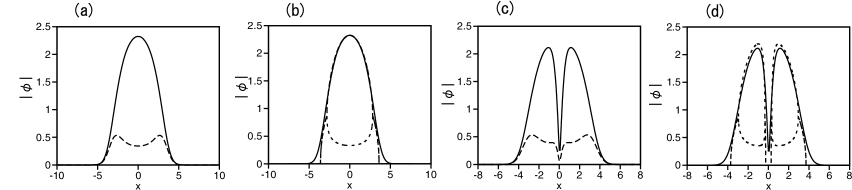
Figure 4: (a) 1D cross sections (radial profiles) of components $\left|\phi_{1}\right|$ ans $\left|\phi_{2}\right|$ (solid and dashed lines, respectively) of the stable 2D ground state ($S=0$) with broken inter-component symmetry. The solution was obtained by means of the imaginary-time-evolution method applied to the axisymmetric reduction of Eqs. (1) and (2) in the 2D form, with $\gamma=2.3$ and $m=1$, for the total 2D norm $N=100$. (b) Comparison of $\left|\phi_{1}\right|$ (the solid line) taken from the same numerical solution as in (a), and its TFA counterpart, produced by Eqs. (24) and (25) (the dashed line which almost completely overlaps with the solid one). The other dashed line shows the TFA-produced component $\left|\phi_{2}\right|$. (c,d): The same as in (a,b), but for a stable vortex mode with $S=1$ and the same values of $\gamma$, $m$, and $N$.

The results are summarized in Figs. 5(a), (b), and (c) by means of curves $R(\gamma)$ for the dependence of asymmetry measure (10) on the cross-component repulsion strength, $\gamma$, for the fixed mass, $m=1$, total norm, $N=100$, and three values of the vorticity, $S=0$ [(a), the GS], $S=1$ (b), and $S=2$ (c). The TFA-predicted analytical results are included too. In particular, for $S=1$ the numerically found SSB point is $\gamma_{S=1}^{\mathrm{(cr)}}\approx 1.55$, while its TFA counterpart, found from Eq. (37), is $\left(\gamma_{S=1}^{\mathrm{(cr)}}\right)_{\mathrm{TFA}}\approx 1.45$. Similar to the conclusion made above for 1D GS [cf. Fig. 1(c)], for all the cases of $S=0$, $1$, and $2$ the SSB transitions, displayed in Figs. 5(a-c), may be categorized as the supercritical bifurcation [53].

In comparison with the similar results for the 1D GS, displayed in Fig. 1(c), the relative error of TFA [in particular, in predicting $\gamma^{\mathrm{(cr)}}$] is much larger in the 2D setting, being $\simeq 5\%$ in 1D and $\simeq 15\%$ in 2D. On the other hand, it is worthy to note that the relative error is smaller by a factor $\simeq 3$ for the vortex states with $S=1$ and $2$, in comparison to the 2D GS.

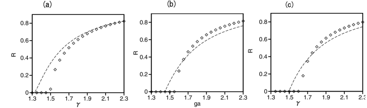
Figure 5: The asymmetry measure (10) vs. the cross-repulsion strength, $\gamma$, for families of 2D states with $S=0$ [the ground state, (a)], $S=1$ (b), and $S=2$ (c), with fixed effective mass, $m=1$, and 2D norm, $N=100$. Chains of rhombuses and dashed curves represent, severally, numerical results produced by the imaginary-time-propagation method, and analytical results provided by TFA, viz., Eqs. (15) and (18) for $S=0$, and Eqs. (24), (25) for $S=1$ and $2$.

Numerical and approximate analytical dependences of the value of $\gamma$ at the SSB point, $\gamma^{\mathrm{(cr)}}$, on the total norm, $N$, for the 2D GS ($S=0$) and vortex mode with $S=1$ are plotted in Fig. 6, fixing the effective mass to be $m=1$. The analytical curves are produced by TFA, i.e., Eq. (22) for $S=0$, and Eq. (37) for $S=1$. In comparison to similar results for the 1D GS, shown in Fig. 2(b), the accuracy of TFA in 2D is only slightly poorer (note, however, a great difference in the scale of $N$ between the 1D and 2D cases).

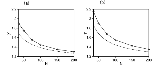
Figure 6: The critical value of the cross-repulsion strength at the symmetry-breaking point in the 2D system, as a function of $N$ at $m=1$. (a) The ground state, $S=0$; (b) the vortex, with $S=1$. The dashed lines denote the TFA prediction, produced, respectively, by Eqs. (22) and (37).

Finally, systematic direct simulations of the perturbed evolution of the 2D states clearly demonstrate that families of the asymmetric GS solutions with $S=0$ and unitary-vortex ones with $S=1$ are completely stable, while asymmetric double vortices, with $S=2$, are not. A typical example of the instability development in displayed in Fig. 7, which shows spontaneous splitting of the double vortex into a pair of unitary ones, that keep the asymmetric structure, with respect to components $\phi_{1}$ and $\phi_{2}$. It is relevant to mention that double vortices may be unstable in the framework of the single GPE with the HO trapping potential and self-repulsive nonlinearity, while unitary vortices are completely stable in the same setting [55].

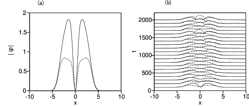
Figure 7: (a) A numerically found 2D stationary state with double vorticity, $S=2$ and broken symmetry between the components. (b) Unstable evolution of this state, leading to its spontaneous splitting in two unitary vortices. The parameters are $m=1$ and $\gamma=1.8$, the total norm of the stationary state being $N=100$. Both the stationary state and the perturbed evolution are displayed by means of 1D cross sections.

4 Spontaneous symmetry breaking (SSB) in two-component gap solitons

Another possibility to create localized states in the presence of a fully repulsive nonlinearity, is offered, instead of the HO trapping potential, by a periodic one – namely, an optical lattice in BEC [47, 48], or a photonic-crystal structure in optics [56, 57]. It is well known that the interplay of the self-repulsion with a periodic potential gives rise to stable gap solitons [59, 58]. The analysis of two-component gap solitons in linearly-coupled dual-core systems with a periodic potential and intrinsic self-repulsive nonlinearity in each layer (in the absence of the inter-component nonlinearity) was developed in Refs. [46, 43, 32]. As mentioned above, symmetric states in such systems are not subject to SSB, while antisymmetric ones develop instability which replaces them by states with broken antisymmetry. Here, we aim to demonstrate that SSB occurs in the coupled system if it includes relatively weak repulsion between the components (instead of the relatively strong inter-component repulsion, which was necessary for the SSB effect considered above in the states trapped in the HO potential).

In the 1D setting, the system of linearly coupled GPEs, including the periodic potential with amplitude $U_{0}$, is written, in the scaled form, as

$$i\frac{\partial\phi_{1}}{\partial t}=-\frac{1}{2}\frac{\partial^{2}\phi_{1}}{\partial x^{2}}-U_{0}\cos\left(2\pi x\right)\phi_{1}+(|\phi_{1}|^{2}+\gamma|\phi_{2}|^{2})\phi_{1}-\epsilon\phi_{2},$$ (38)

$$i\frac{\partial\phi_{2}}{\partial t}=-\frac{1}{2}\frac{\partial^{2}\phi_{2}}{\partial x^{2}}-U_{0}\cos\left(2\pi x\right)\phi_{2}+(|\phi_{2}|^{2}+\gamma|\phi_{1}|^{2})\phi_{2}-\epsilon\phi_{1}.$$ (39)

Here, the period of the potential is fixed to be $1$, and, to clearly demonstrate the SSB effects, it is convenient to fix the linear-coupling constant as $\epsilon=0.05$, instead of $\epsilon=1$ in Eqs. (1), (2).

To develop an analytical approach to the study of the gap solitons, we resort to the averaging method [60], which looks for solutions in the form of a rapidly oscillating carrier wave, with the period equal to the double period of the lattice potential, modulated by slowly varying (envelope) wave functions, $\Phi_{1,2}(x,t)$:

$$\phi_{1,2}\left(x,t\right)=\Phi_{1,2}\left(x,t\right)\cos\left(\pi x\right).$$ (40)

It is known that this approach makes it possible to predict gap solitons existing close to edges of the spectral bandgap. The substitution of this ansatz in Eqs. (38) and (39) and application of the averaging procedure leads, in the lowest approximation, to the following system of equations for the slowly varying wave functions:

$$i\frac{\partial\Phi_{1}}{\partial t}=-\frac{1}{2m_{\mathrm{eff}}}\frac{\partial^{2}\Phi_{1}}{\partial x^{2}}+\frac{3}{4}(|\Phi_{1}|^{2}+\gamma|\Phi_{2}|^{2})\Phi_{1}-\epsilon\Phi_{2},$$ (41)

$$i\frac{\partial\Phi_{2}}{\partial t}=-\frac{1}{2m_{\mathrm{eff}}}\frac{\partial^{2}\Phi_{2}}{\partial x^{2}}+\frac{3}{4}(|\Phi_{2}|^{2}+\gamma|\Phi_{1}|^{2})\Phi_{2}-\epsilon\Phi_{1},$$ (42)

where the effective mass is

$$m_{\mathrm{eff}}=|U_{0}|/(|U_{0}|-2\pi^{2}).$$ (43)

At $U_{0}<2\pi^{2}$, the effective mass is negative, hence its interplay with the repulsive sign of the nonlinearity in Eqs. (41) and (42) gives rise to bright solitons, similar to how usual solitons are produced by the balance of the positive mass and attractive nonlinearity.

To use the results reported in Ref. [34], it is convenient to additionally rescale the variables in Eqs. (41) and (42), defining $t^{\prime}=-\epsilon t$, $x^{\prime}=\sqrt{-m_{\mathrm{eff}}\epsilon}x$, and

$$\Phi_{1}^{\prime}=\sqrt{4\epsilon/(3\gamma)}\Phi_{1},\Phi_{2}^{\prime}=-\sqrt{4\epsilon/(3\gamma)}\Phi_{2},$$ (44)

thus replacing Eqs. (41) and (42) by

$$i\frac{\partial\Phi_{1}^{\prime}}{\partial t^{\prime}}=-\frac{1}{2}\frac{\partial^{2}\Phi_{1}^{\prime}}{\partial x^{\prime 2}}-\left(\frac{1}{\gamma}|\Phi_{1}^{\prime}|^{2}+|\Phi_{2}^{\prime}|^{2}\right)\Phi_{1}^{\prime}-\Phi_{2}^{\prime}.$$ (45)

$$i\frac{\partial\Phi_{2}^{\prime}}{\partial t^{\prime}}=-\frac{1}{2}\frac{\partial^{2}\Phi_{2}^{\prime}}{\partial x^{\prime 2}}-\left(\frac{1}{\gamma}|\Phi_{2}^{\prime}|^{2}+|\Phi_{1}^{\prime}|^{2}\right)\Phi_{2}^{\prime}-\Phi_{1}^{\prime}.$$ (46)

Accordingly, the total norm of rescaled fields $\Phi_{1,2}^{\prime}$ is related to the norm of the original ones, $\Phi_{1,2}$:

$$N^{\prime}=(3\gamma/4)\sqrt{m_{\mathrm{eff}}/\epsilon}N.$$ (47)

As shown in Ref. [34], Eqs. (45) and (46) with $\gamma<1$ give rise to SSB of symmetric solitons, in terms of this system, i.e., ones with $\Phi_{1}^{\prime}=\Phi_{2}^{\prime}$, if $\gamma$ belongs to interval $\gamma<\left(\gamma^{\prime}\right)^{\mathrm{(cr)}}$, where the respective critical value is related to $N^{\prime}$ by equation

$$N^{\prime}=\frac{256\left[1/\left(\gamma^{\prime}\right)^{\mathrm{(cr)}}+1\right]^{-1}}{\left[\sqrt{25/\left(\gamma^{\prime}\right)^{\mathrm{(cr)}}-7}-3\sqrt{1/\left(\gamma^{\prime}\right)^{\mathrm{(cr)}}+1}\right]\left[\sqrt{25/\left(\gamma^{\prime}\right)^{\mathrm{(cr)}}-7}+\sqrt{1/\left(\gamma^{\prime}\right)^{\mathrm{(cr)}}+1}\right]}.$$ (48)

Actually, Eq. (44) implies that the solitons subject to constraint $\Phi_{1}^{\prime}=\Phi_{2}^{\prime}$ represent antisymmetric solitons, with $\Phi_{2}(x)=-\Phi_{1}(x)$, in terms of the original equations (41) and (42).

Numerical solutions for asymmetric solitons can be readily generated by the imaginary-time integration method applied to Eqs. (41) and (42). Figure 8(a) shows an example of a soliton with broken antisymmetry, obtained at parameters $\gamma=0.2$, $U_{0}=5$, $\epsilon=0.05$, and $N=2.5$. Note that the signs of the two components are opposite, in accordance with what is said above, and the breaking of the antisymmetry is exhibited by the difference of their amplitudes. Further, Fig. 8(b) summarizes the results, by displaying the asymmetry measure $R$ for the soliton family, defined as per Eq. (10) with $\left|\varphi_{1}\right|^{2}$ replaced by $\left|\Phi_{1}\right|^{2}$, and $N$ replaced by the total norm defined in terms of envelope wave functions $\Phi_{1,2}$, versus the relative strength $\gamma$ of the inter-component repulsion. The $R(\gamma)$ dependence is plotted for fixed $N=2.5$ and the potential’s amplitude, $U_{0}=5$, hence the respective effective mass, given by Eq. (43), is $m_{\mathrm{eff}}\approx$ $-0.34$. As shown in Ref. [34], the $R(\gamma)$ dependence may be accurately represented by means of a variational approximation. It is seen in Fig. 8(b) that the antisymmetry of the two-component gap solitons is broken at $\gamma<\gamma^{\mathrm{(cr)}}\approx 0.28$. The respective analytical result, determined by Eq. (48) is $\left(\gamma^{\prime}\right)^{\mathrm{(cr)}}\simeq 0.272$, which is consistent with the numerical findings.

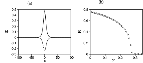
Figure 8: (a) Profiles of $\Phi_{1}$ and $\Phi_{2}$ (solid and dashed lines, respectively), obtained as a numerical solution to Eqs. (41) and (42), representing the two-component soliton with broken antisymmetry, for $U_{0}=5$, $\epsilon=0.05$, and total norm $N=2.5$. (b) The asymmetry measure $R(\gamma)$, defined for the family of the two-component solitons, as produced by the numerical solution for $U_{0}=5$, $\epsilon=0.05$, and total norm $N=2.5$.

The prediction of the breaking of antisymmetry in two-component gap solitons was confirmed by direct simulations of underlying equations (38) and (39), see an example shown in Figs. 9(a)-(c) for $\gamma=0.1<\gamma^{\mathrm{(cr)}}$. The initial conditions were taken as per ansatz (40):

$$\phi_{1,2}(x,t=0)=\Phi_{1,2}(x,t=0)\cos(\pi x),$$ (49)

where $\Phi_{1,2}(x,t)$ is the above-mentioned numerically exact broken-antisymmetry soliton solution of Eqs. (41) and (42), obtained by means of the imaginary-time simulations. Figures 9(a) and (b) show, severally, the resulting evolution of maximum values of $|\phi_{1,2}(x)|$, and of the asymmetry measure, $R$, defined according to Eq. (10). Periodic small-amplitude variations of the fields and asymmetry are caused by a deviation of ansatz (40) from a numerically exact form of the two-component gap soliton with broken inter-component antisymmetry. A nearly exact shape of both components of the gap soliton is produced in Fig. 9(c), which displays snapshots of $|\phi_{1,2}(x)|$ at $t=500$. These numerical results also demonstrate that the gap solitons with broken antisymmetry are stable. Similar to the structure of the asymmetric localized states produced by Eqs. (8) and (9) in the presence of the HO trapping potential, see Fig. 1(a), the two-component gap solitons feature broken antisymmetry in the central zone, and persistent approximate antisymmetry in decaying tails.

Thus, an essential difference from the results reported above for the localized states, trapped in the 1D or 2D HO potential, is that the SSB transition, revealed by Fig. 8(b), is categorized as an inverted bifurcation [53] (alias an extreme subcritical bifurcation, cf. Ref. [61]), in comparison with the supercritical bifurcations observed in Figs. 1(c) and 5. The inversion is explained by the fact that effective mass (43), which drives the bifurcation of the gap solitons, is negative. Another obvious difference is that the two-component antisymmetric gap solitons undergo SSB at $\gamma<1$, on the contrary to the above condition, $\gamma>1$, which is necessary to impose SSB onto the HO-trapped states. On the other hand, it is known that, in the interval of $1<\gamma<3$, the system of Eqs. (41) and (42) gives rise to a bifurcation which breaks symmetry of two-component solitons with $\Phi_{1}=\Phi_{2}$ (the symmetric state, rather than the antisymmetric one considered here) [34]. The consideration of the latter effect in terms of Eqs. (38) and (39) is beyond the scope of the present paper.

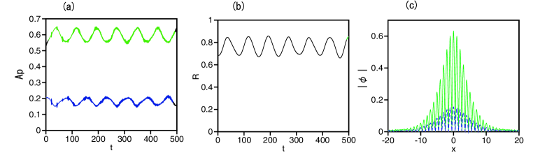
Figure 9: (a) The evolution of maximum values of $|\phi_{1}(x)|$ and $\left|\phi_{2}(x)\right|$ (green and blue lines), as produced by direct simulations of Eqs. (38) and (39), initiated by the input in the form of ansatz (49), with $\Phi_{1,2}$ taken as a numerically exact broken–antisymmetry soliton solution of Eqs. (41) and (42) with $\gamma=0.1$. (b) The evolution of the asymmetry measure for the solution from panel (a), defined as per Eq. (10). (c) Snapshots of $|\phi_{1}(x)|$ and $\left|\phi_{2}(x)\right|$ (green and blue lines, respectively) of the solution from panels (b,c) at $t=500$. The snapshots closely approximate an exact shape of the two-component gap soliton with broken antisymmetry between the components.

5 Conclusion

In numerous works, SSB (spontaneous symmetry breaking) of two-component localized modes in linearly-coupled systems was found in the case of attractive self- and/or cross-component nonlinear interactions in the system. On the contrary to that, in systems with repulsive interactions spontaneous breaking was only shown for antisymmetric two-component states, but not for symmetric ones. Here, we have demonstrated that SSB in both 1D and 2D symmetric states, trapped in the confining potential [taken as the HO (harmonic oscillator)], is possible if the cross-repulsion is stronger than intrinsic repulsion in each component. This setting may be realized in BEC and nonlinear optics. In the former case, it represents a binary condensate with natural repulsive contact interactions and radiofrequency-induced linear mixing between two atomic states, which compose the binary BEC. In terms of self-defocusing optical waveguides, the system is based on the copropagation of two orthogonal polarizations of light with the linear mixing induced by linear-polarization birefringence of the material.

For both one- and two-dimensional GSs (ground states), as well as for 2D vortex states, the transition from symmetric states to asymmetric ones has been demonstrated analytically by means of TFA (Thomas-Fermi approximation) and confirmed by systematically collected numerical solutions of the underlying system of linearly coupled GPEs (Gross-Pitaevskii equations). A characteristic feature of the asymmetric states is that they combine strongly broken asymmetry in the inner area, while a surrounding layer keeps the original symmetry, in the approximate form. The SSB transition for all these states is identified as a supercritical bifurcation. It produces stable 1D and 2D asymmetric GSs, as well as stable asymmetric vortices with topological charge $S=1$, while the vortices with $S=2$ are unstable against splitting in a pair of unitary vortices.

The phenomenology of the spontaneous antisymmetry breaking was also briefly considered for 1D antisymmetric two-component gap solitons, maintained by the spatially periodic potential. In this case, the antisymmetry breaks in the inner region of the gap soliton under the condition opposite to that necessary for the occurrence of the SSB effect in the HO-trapped modes, viz., the cross-component repulsion must be weaker than the self-repulsion in each component. The character of the antisymmetry-breaking transition for the gap solitons is opposite too, namely, it amounts to an inverted bifurcation.

The above analysis did not address motion of the trapped modes. Application of a kick to the 1D trapped state, as well as of a radial push to 2D ones, should excite a dipole mode of oscillations of the perturbed states around the center. In this connection, the effect of the Rabi coupling on the oscillations may be an interesting feature, as suggested by recently studied effects of the same term on the motion of spinor solitons in a random potential [62]. Gap solitons feature mobility too, with a negative dynamical mass [63], and, accordingly, it may be interesting to address an effect of the Rabi coupling on the motion of two-component gap solitons.

This work can be also extended by considering higher-order (first of all, dipole) spatial modes in the system with the HO trapping potential, as well as antisymmetric and symmetric two-component configurations in the cases of the HO and periodic potentials, respectively. A challenging possibility is to develop the analysis for the three-dimensional version of the BEC model.

References

- [1] Spontaneous Symmetry Breaking, Self-Trapping, and Josephson Oscillations, ed. by B. A. Malomed (Springer-Verlag: Berlin and Heidelberg, 2013).
- [2] L. D. Landau and E. M. Lifshitz, Quantum Mechanics (Moscow: Nauka Publishers, 1974).
- [3] E. B. Davies, Symmetry breaking in a non-linear Schrödinger equation, Commun. Math. Phys. 64, 191-210 (1979).
- [4] J. C. Eilbeck, P. S. Lomdahl, and A. C. Scott, The discrete self-trapping equation, Physica D 16, 318-338 (1985).
- [5] Y. S. Kivshar and G. P. Agrawal, Optical Solitons: From Fibers to Photonic Crystals (Academic Press: San Diego).
- [6] L. P. Pitaevskii, S. Stringari, Bose-Einstein Condensation (Oxford University Press: Oxford, 2003).
- [7] H. T. C. Stoof, K. B. Gubbels, and D. B. M. Dickrsheid, Ultracold Quantum Fields (Springer: Dordrecht, 2009).
- [8] S. Trillo, S. Wabnitz, E. M. Wright, and G. I. Stegeman, Soliton switching in fiber nonlinear directional couplers. Opt. Lett. 13, 672–674 (1988).
- [9] E. M. Wright, G. I. Stegeman, and S. Wabnitz, Solitary-wave decay and symmetry-breaking instabilities in two-mode fibers, Phys. Rev. A 40, 4455-4466 (1989).
- [10] C. Paré and M. Fłorjańczyk, Approximate model of soliton dynamics in all-optical couplers, Phys. Rev. A 41, 6287-6295 (1990).
- [11] A. W. Snyder, D. J. Mitchell, L. Poladian, D. R. Rowland, and Y. Chen, Physics of nonlinear fiber couplers, J. Opt. Soc. Am. B 8, 2101-2118 (1991).
- [12] A. I. Maimistov, Propagation of a light pulse in nonlinear tunnel-coupled optical waveguides, Kvant. Elektron. 18, 758-761 (1990) [Sov. J. Quantum Electron. 21, 687-690 (1991)].
- [13] M. Romagnoli, S. Trillo, and S. Wabnitz, Soliton switching in nonlinear couplers, Opt. Quantum Electron 24, S1237–S1267 (1992).
- [14] P. L. Chu, B. A. Malomed, and G. D. Peng, Soliton switching and propagation in nonlinear fiber couplers: analytical results, J. Opt. Soc. Am. B 10, 1379-1385 (1993).
- [15] N. Akhmediev and A. Ankiewicz, Novel soliton states and bifurcation phenomena in nonlinear fiber couplers, Phys. Rev. Lett. 70, 2395-2398 (1993).
- [16] G. L. Diankov, I. M. Uzunov, and F. Lederer, Effect of 3rd-order dispersion on pulse dynamics in nonlinear directional coupler, Electr. Lett. 30, 155-156 (1994).
- [17] I. M. Uzunov, R. Muschall, M. Goelles, Yu. S. Kivshar, B. A. Malomed, and F. Lederer, Pulse switching in nonlinear fiber directional couplers. Phys. Rev. E 51, 2527-2537 (1995).
- [18] W. C. K. Mak, B. A. Malomed, and P. L. Chu, Solitary waves in coupled nonlinear waveguides with Bragg gratings, J. Opt. Soc. Am. B 15, 1685-1692 (1998).
- [19] J. F. Jia, Y. P. Zhang, W. D. Li, and L. Li, Optical modes in a nonlinear double-channel waveguide, Opt. Commun. 283, 132-137 (2010).
- [20] D. A. Smirnova, A. V. Gorbach, I. V. Iorsh, I. V. Shadrivov, and Y. G. Kivshar, Nonlinear switching with a graphene coupler, Phys. Rev. B 88, 045443 (2013).
- [21] M. J. Islam and J. Atai, Stability of gap solitons in dual-core Bragg gratings with cubic-quintic nonlinearity, Laser Phys. Lett. 12, 015401 (2015).
- [22] B. A. Malomed, Solitons and nonlinear dynamics in dual-core optical fibers, In: Handbook of Optical Fibers, ed. by G.-D. Peng (Springer-Nature, Singapore, 2019).
- [23] F. Diebel, D. Leykam, M. Boguslawski, P. Rose, C. Denz, and A. Desyatnikov, All-optical switching in optically induced nonlinear waveguide couplers, Appl. Phys. Lett. 104, 261111 (2014).
- [24] M. Longobucco, J. Cimek, L. Curilla, D. Pysz, P. Buczynski, and I. Bugar, All-optical switching based on soliton self-trapping in dual-core high-contrast optical fibre, Opt. Fiber Tech. 51, 48-58 (2019).
- [25] S. M. Jensen, The non-linear coherent coupler, IEEE J. Quant. Elect. 18, 1580-1583 (1982).
- [26] Y. Li, W. Pang, S. Fu, and B. A. Malomed, Two-component solitons under a spatially modulated linear coupling: Inverted photonic crystals and fused couplers, Phys. Rev. A 85, 053821 (2012).
- [27] T. Heil, I. Fischer, W. Elsässer, J. Mulet, and C. R. Mirasso, Chaos synchronization and spontaneous symmetry-breaking in symmetrically delay-coupled semiconductor lasers, Phys. Rev. Lett. 86, 795-798 (2000).
- [28] S. Haddadi, A. M. Yacomotti, I. Sagnes, F. Raineri, G. Beaudoin, L. Le Gratiet, and J. A. Levenson, Photonic crystal coupled cavities with increased beaming and free space coupling efficiency, Appl. Phys. Lett. 102, 011107 (2013).
- [29] P. Hamel, S. Haddadi, F. Raineri, P. Monnier, G. Beaudoin, I. Sagnes, A. Levenson, and A. M. Yacomotti, Spontaneous mirror-symmetry breaking in coupled photonic-crystal nanolasers, Nature Phot. 9, 311-315 (2015).
- [30] B. A. Malomed, Symmetry breaking in laser cavities, Nature Phot. 9, 287-289 (2015).
- [31] M. Matuszewski, B. A. Malomed, and M. Trippenbach, Spontaneous symmetry breaking of solitons trapped in a double-channel potential, Phys. Rev. A 75, 063621 (2007).
- [32] M. Trippenbach, E. Infeld, J. Gocalek, M. Matuszewski, M. Oberthaler, and B. A. Malomed, Spontaneous symmetry breaking of gap solitons in double-well traps, Phys. Rev. A 78, 013603 (2008).
- [33] L. Salasnich, B. A. Malomed, and F. Toigo. Competition between the symmetry breaking and onset of collapse in weakly coupled atomic condensates, Phys. Rev. A 81, 045603 (2010).
- [34] H. Sakaguchi and B. A. Malomed, Symmetry breaking of solitons in two-component Gross-Pitaevskii equations, Phys. Rev. E 83, 036608 (2011).
- [35] M. Abad and A. Recati, A study of coherently coupled two-component Bose-Einstein condensates, Eur. Phys. J. D 67, 148 (2013).
- [36] X. M. Xi, T. Weiss, G. K. L. Wong, F. Biancalana, S. M. Barnett, M. J. Padgett, and P. St. J. Russell, Optical activity in twisted solid-core photonic crystal fibers, Phys. Rev. Lett. 110, 143903 (2013).
- [37] R. J. Ballagh, K. Burnett, and T. F. Scott, Theory of an output coupler for Bose-Einstein condensed atoms, Phys. Rev. Lett. 78, 1607-1611 (1997).
- [38] P. Öhberg and S. Stenholm, Internal Josephson effect in trapped double condensates, Phys. Rev. A 59, 3890-3895 (1999).
- [39] D. T. Son and M. A. Stephanov, Domain walls of relative phase in two-component Bose-Einstein condensates, Phys. Rev. A 65, 063621 (2002).
- [40] S. D. Jenkins and T. A. Kennedy, Dynamic stability of dressed condensate mixtures, Phys. Rev. A 68, 053607 (2003).
- [41] M. I. Merhasin, B. A. Malomed, and R. Driben, Transition to miscibility in a binary Bose-Einstein condensate induced by linear coupling, J. Physics B 38, 877-892 (2005).
- [42] N. Dror and B. A. Malomed, Symmetric and asymmetric solitons and vortices in linearly coupled two-dimensional waveguides with the cubic-quintic nonlinearity, Physica D 240, 526-541 (2011).
- [43] A. Gubeskys and B. A. Malomed, Spontaneous soliton symmetry breaking in two-dimensional coupled Bose-Einstein condensates supported by optical lattices, Phys. Rev. A 76, 043623 (2007).
- [44] L. Salasnich and B. A. Malomed, Spontaneous symmetry breaking in linearly coupled disk-shaped Bose-Einstein condensates, Molecular Phys. 109, 2737-2745 (2011).
- [45] Z. Chen, Y. Li, B. A. Malomed, and L. Salasnich, Spontaneous symmetry breaking of fundamental states, vortices, and dipoles in two and one-dimensional linearly coupled traps with cubic self-attraction, Phys. Rev. A 96, 033621 (2016).
- [46] A. Gubeskys and B. A. Malomed, Symmetric and asymmetric solitons in linearly coupled Bose-Einstein condensates trapped in optical lattices, Phys. Rev. A 75, 063602 (2007).
- [47] B. Eiermann, Th. Anker, M. Albiez, M. Taglieber, P. Treutlein, K.-P. Marzlin, and M. K. Oberthaler, Bright Bose-Einstein gap solitons of atoms with repulsive interaction, Phys. Rev. Lett. 92, 230401 (2004).
- [48] O. Morsch and M. Oberthaler, Dynamics of Bose-Einstein condensates in optical lattices, Rev. Mod. Phys. 78, 179 (2006).
- [49] V. P. Mineev, Theory of solution of two almost perfect Bose gases, Zh. Eksp. Teor. Fiz. 67, 263-272 (1974) [English translation: Sov. Phys. JETP 40, 132 (1974)].
- [50] G. P. Agrawal, Modulation instability induced by cross-phase modulation, Phys. Rev. Lett. 59, 880-883 (1987).
- [51] M. L. Chiofalo, S. Succi, and M. P. Tosi, Ground state of trapped interacting Bose-Einstein condensates by an explicit imaginary-time algorithm. Phys. Rev. E 62, 7438-7444 (2000).
- [52] W. Bao and Q. Du, Computing the ground state solution of Bose-Einstein condensates by a normalized gradient flow, SIAM J. Sci. Comput. 25, 1674-1697 (2004).
- [53] G. Iooss and D. D. Joseph, Elementary Stability Bifurcation Theory (Springer-Verlag: New York, 1980).
- [54] A. L. Fetter, Rotating trapped Bose-Einstein condensates, Rev. Mod. Phys. 81, 641-691 (2009).
- [55] H. Pu, C. K. Law, J. H. Eberly, and N. P. Bigelow, Coherent disintegration and stability of vortices in trapped Bose condensates, Phys. Rev. A 59, 1533 (1999).
- [56] J. D Joannopoulos, S. G. Johnson, J. N. Winn, and R. D. Meade, Photonic Crystals: Molding the Flow of Light (Princeton University Press: Princeton and Oxford, 2008).
- [57] M. Skorobogatiy and J. Yang, Fundamentals of Photonic Crystal Guiding (Cambridge University Press: Cambridge, 2009).
- [58] V. A. Brazhnyi and V. V. Konotop, Theory of nonlinear matter waves in optical lattices, Mod. Phys. Lett. B 18, 627-651 (2004).
- [59] W. Chen and D. L. Mills, Gap solitons and the nonlinear optical-response of superlattices, Phys. Rev. Lett. 58, 160-163 (1987).
- [60] B. B. Baizakov, V. V. Konotop, and M. Salerno, Regular spatial structures in arrays of Bose-Einstein condensates induced by modulational instability, J. Phys. B: At. Mol. Opt. Phys. 35, 5105-5119 (2002).
- [61] T. Mayteevarunyoo, B. A. Malomed, and G. Dong, Spontaneous symmetry breaking in a nonlinear double-well structure, Phys. Rev. A 78, 053601 (2008).
- [62] Sh. Mardonov, M. Modugno, E. Ya. Sherman, and B. A. Malomed, Rabi-coupling-driven motion of a soliton in a Bose-Einstein condensate, Phys. Rev. A 99, 013611 (2019).
- [63] H. Sakaguchi and B. A. Malomed, Dynamics of positive- and negative-mass solitons in optical lattices and inverted traps, J. Phys. B: At. Mol. Opt. Phys. 37, 1443-1459 (2004).