On the Period–Luminosity–Metallicity relation of Classical Cepheids

Abstract

Context. Classical Cepheids (DCEPs) are the most important primary indicators for the extragalactic distance scale. Establishing the dependence on metallicity of their period–luminosity and period–Wesenheit (PL/PW) relations has deep consequences on the estimate of the Hubble constant (H₀).

Aims. We aim at investigating the dependence on metal abundance ([Fe/H]) of the PL/PW relations for Galactic DCEPs.

Methods. We combined proprietary and literature photometric and spectroscopic data, gathering a total sample of 413 Galactic DCEPs (372 fundamental mode – DCEP_F and 41 first overtone – DCEP_1O) and constructed new metallicity-dependent PL/PW relations in the near infra-red (NIR) adopting the Astrometric Based Luminosity.

Results. We find indications that the slopes of the PL$(K_{s})$ and PW$(J,K_{S})$ relations for Galactic DCEPs might depend on metallicity when compared to the Large Magellanic Cloud relationships. Therefore, we have used a generalized form of the PL/PW relations to simultaneously take into account the metallicity dependence of the slope and intercept of these relations.

Conclusions. We calculated PL/PW relations which, for the first time, explicitly include a metallicity dependence of both the slope and intercept terms. Although the insufficient quality of the available data makes our results not yet conclusive, they are relevant from a methodological point of view. The new relations are linked to the geometric measurement of the distance to the Large Magellanic Cloud and allowed us to estimate a Gaia DR2 parallax zero point offset $\Delta\varpi$=0.0615$\pm$0.004 mas from the dataset of DCEPs used in this work.

1 Introduction

Classical Cepheids (DCEPs) are the most important primary distance indicators of the cosmic distance ladder thanks to their Period-Luminosity (PL, Leavitt & Pickering, 1912) and Period-Wesenheit (PW, Madore, 1982) relations. Indeed, once calibrated locally by means of geometric methods such as trigonometric parallaxes, the PL/PW relations can be used to calibrate secondary distance indicators such as Type Ia Supernovae (SNe), which are sufficiently powerful to measure distances in the unperturbed Hubble flow. Eventually, this three-step procedure allows us to measure the Hubble constant (H₀) from the slope of the relation between the distance to far away galaxies in the Hubble flow and their recession velocity (e.g. Sandage et al. 2006; Freedman, & Madore 2011; Freedman et al. 2012; Riess et al. 2016, 2019).

The value of H₀ is presently a matter of vivid debate in the literature because the most recent determinations based on the cosmic distance ladder, H₀=74.03$\pm$1.42 km s^-1 Mpc^-1 (Riess et al. 2019 and references therein) significantly disagree with the value of H₀ estimated from the Planck Cosmic Microwave Background (CMB) measurements under the flat $\Lambda$ Cold Dark Matter ($\Lambda$CDM) model, H₀=67.4$\pm$0.5 km s^-1 Mpc^-1 (Planck Collaboration et al., 2018). This 4.4$\sigma$ discrepancy, commonly referred to as the H₀ tension, remains unexplained notwithstanding several attempts to reduce the systematic errors affecting the different steps of the cosmic distance ladder (e.g. Huang et al., 2020; Yuan et al., 2019; Reid et al., 2019). Recently, a value of H${}_{0}=73.3^{+1.7}_{-1.8}$ km s^-1 Mpc^-1, in agreement with the cosmic distance ladder, was obtained by the H0LICOW and STRIDES collaborations based on the gravitational time-delays of six lensed quasars (Wong et al., 2020). Since this measurement is totally independent of the cosmic distance ladder calibrations, the occurrence of a tension appears to be confirmed. In order to improve the accuracy of the H₀ measurements and to put stringent constraints on cosmological models, it is crucial to quantify the residual systematic errors affecting different methods to estimate H₀. In particular, it is mandatory to quantify and reduce the uncertainties (random and systematic) of the different steps involved in the distance ladder calibration.

One of the main residual source of uncertainty in the cosmic distance ladder is the metallicity dependence of the DCEP PL/PW relations. Indeed, the metallicity is widely expected to affect both the slope and intercept of the DCEP $PL/PW$ relations, particularly at optical passbands. Conversely, the metallicity dependence of the DCEP PW relations is estimated and predicted to be small for different band combinations but especially in the near infra-red (NIR, see e.g. Fiorentino et al., 2007; Ngeow et al., 2012b; Di Criscienzo et al., 2013; Fiorentino et al., 2013; Gieren et al., 2018, and references therein). The procedure adopted by the SH0ES team (Riess et al., 2016) to calibrate the cosmic distance ladder, takes into account the metallicity dependence of the PW relations. According to these authors, the metallicity contributes a 0.5% to the total error budget of 2.4% in the measure of H₀. However, there is a significant disagreement among estimates for the metallicity dependence of the PL/PW relations obtained by different authors (e.g. Macri et al., 2006; Romaniello et al., 2008; Bono et al., 2010; Freedman, & Madore, 2011; Shappee, & Stanek, 2011; Pejcha, & Kochanek, 2012; Groenewegen, 2013; Kodric et al., 2013; Fausnaugh et al., 2015; Riess et al., 2016). This variety of results can be partially explained by the significant errors still affecting the metal abundances of DCEPs in the distant galaxies which are addressed in these studies.

A direct determination of the metallicity effect on the Cepheid distance scale, based on Galactic DCEPs with [Fe/H] abundances obtained from high-resolution spectroscopy, has been hampered until recently by the lack of precise distance measurements for a sufficiently large number of MW DCEPs. In this context, a unique contribution is nowadays being provided by the Gaia mission (Gaia Collaboration et al., 2016) which published in its Data Release 2 (DR2) precise parallaxes for hundreds of MW DCEPs, including most of the new discoveries in the last couple of years (see e.g. Chen et al., 2018; Jayasinghe et al., 2018; Udalski et al., 2018; Clementini et al., 2019; Ripepi et al., 2019). Further improved parallaxes are foreseen to be provided by future Gaia data releases.

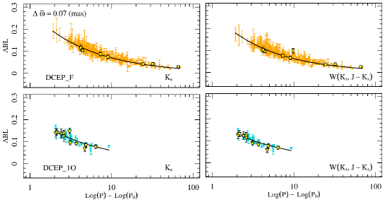
Figure 1: Results of the fitting procedure for an ABL in the form of Eq. 1 (left) and Eq. 2 (right) for DCEP_Fs (top panels) and DCEP_1Os (bottom panels) and a Gaia zero point parallax offset of $\Delta\varpi=0.07$ mas. Orange and cyan filled circles represent the literature data for F and 1O MW DCEPs, respectively. Yellow-filled squares and triangles display the DCEP_Fs and DCEP_1Os analysed in Paper I, respectively. For clarity reasons, outliers were not shown.

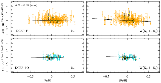
Figure 2: Results of the fitting procedure for an ABL in the form of Eq. 3 (left) and Eq. 4 (right) for DCEP_Fs (top panels) and DCEP_1Os (bottom panels) and a Gaia zero point parallax offset of $\Delta\varpi=0.07$ mas. Symbols are as in Fig. 1

However, only a small fraction of the recently discovered DCEPs have accurate multiband photometry and spectroscopic abundances. Therefore, to fully exploit the potential of such an ideal amount of data and better estimate the metallicity dependence of the DCEP PL/PW relations, it is crucial to increase the sample of well characterized (both in photometry and spectroscopy) MW DCEPs. To this end, we are carrying out a project which foresees the combination of multiband photometry availble in the literature with metal abundances from newly acquired high-resolution spectroscopy for more than a hundred MW DCEPs, selected among the new discoveries and those poorly characterized in the literature so far. First results from this project were published in Catanzaro et al. (2020), where we present a new lithium-rich DCEP, V363 Cas, the fifth of such a rare class of DCEPs to be discovered in the MW, and in Ripepi et al. (A&A submitted, hereinafter Paper I) where we present elemental abundances from high-resolution spectroscopy for a first sample of 21 DCEPs and a Type II Cepheid of BL Herculis (BL Her) type among the more than 100 DCEPs we are targeting with our observing program.

In this paper we exploit the iron abundances published in Paper I along with literature data to study the metallicity dependence of the NIR PL/PW relations for MW DCEPs.

2 The sample

In Paper I we presented chemical abundances and photometric properties for a sample of 21 DCEPs and one BL Her star. This sample was complemented with homogeneous literature data from Gaia Collaboration et al. (2017) and Groenewegen (2018). A detailed description of the properties of our total sample can be found in Paper I. Here we only recall that it consists of 389 fundamental mode (DCEP_F) and 44 first overtone (DCEP_1O) classical Cepheids. Among them, those with RUWE$\geq 1.4$ were discarded as recommended by the Gaia documentation. Similarly, we removed the DCEPs with $V<6$ mag, as their Gaia parallaxes are too uncertain (see Riess et al., 2018). The literature sample hence reduced to 364 DCEP_F and 38 DCEP_1O pulsators. Adding the 9 DCEP_F and 12 DCEP_1O pulsators studied in Paper I, our final sample consisting of 373 DCEP_Fs and 50 DCEP_1Os.

Table 1: Results from the least square fit of an ABL function in the form of Eqs. 1 and  2 (upper portion of the table); Eqs. 3 and  4 (middle portion of the table), or Eqs. 5 and  6 (lower part of the table). The functional form of the PW relation is labelled in the table. $P_{0}$ is the pivoting period, whose logarithm is equal to 1.0 and 0.3 for DCEP_Fs and DCEP_1Os, respectively.

$\alpha$	$\beta$	$\gamma$	$\delta$	n	nrej	Mode	$\Delta\varpi$	Case	$\sigma_{\rm ABL}$	AIC
(1)	(2)	(3)	(4)	(5)	(6)	(7)	(8)	(9)	(10)	(11)
$M_{K_{S,0}}$ or $W(J,K_{S})=\alpha+\beta(\log P-\log P_{0})$
$-5.840\pm 0.023$	$-3.061\pm 0.070$	–	–	373	47	F	0.0490	(K)	0.0095	$-$2594
$-5.794\pm 0.021$	$-3.027\pm 0.090$	–	–	373	55	F	0.0615	(K)	0.0091	$-$2533
$-5.762\pm 0.028$	$-3.012\pm 0.086$	–	–	373	53	F	0.0700	(K)	0.0098	$-$2533
$-6.131\pm 0.027$	$-3.219\pm 0.078$	–	–	373	45	F	0.0490	(K, JK)	0.0091	$-$2666
$-6.072\pm 0.024$	$-3.185\pm 0.085$	–	–	373	51	F	0.0615	(K, JK)	0.0086	$-$2635
$-6.027\pm 0.016$	$-3.200\pm 0.087$	–	–	373	40	F	0.0700	(K, JK)	0.0090	$-$2631
$-4.223\pm 0.082$	$-2.836\pm 0.474$	–	–	50	2	1O	0.0490	(K)	0.0109	$-$366
$-4.190\pm 0.117$	$-2.788\pm 0.533$	–	–	50	2	1O	0.0615	(K)	0.0101	$-$364
$-4.166\pm 0.091$	$-2.780\pm 0.453$	–	–	50	2	1O	0.0700	(K)	0.0107	$-$365
$-4.457\pm 0.101$	$-2.889\pm 0.425$	–	–	50	2	1O	0.0490	(K, JK)	0.0091	$-$382
$-4.430\pm 0.092$	$-2.786\pm 0.371$	–	–	50	5	1O	0.0615	(K, JK)	0.0078	$-$363
$-4.404\pm 0.082$	$-2.802\pm 0.428$	–	–	50	4	1O	0.0700	(K, JK)	0.0087	$-$370
$M_{K_{S,0}}$ or $W(J,K_{S})=\alpha+\beta(\log P-\log P_{0})+\gamma{\rm[Fe/H]}$
$-5.837\pm 0.030$	$-3.053\pm 0.093$	$-0.039\pm 0.151$	–	373	46	F	0.0490	(K)	0.0096	$-$2600
$-5.785\pm 0.027$	$-3.015\pm 0.089$	$-0.082\pm 0.138$	–	373	55	F	0.0615	(K)	0.0091	$-$2532
$-5.746\pm 0.022$	$-2.992\pm 0.077$	$-0.141\pm 0.140$	–	373	54	F	0.0700	(K)	0.0098	$-$2527
$-6.121\pm 0.027$	$-3.216\pm 0.067$	$-0.084\pm 0.145$	–	373	41	F	0.0490	(K, JK)	0.0093	$-$2684
$-6.033\pm 0.029$	$-3.171\pm 0.065$	$-0.284\pm 0.115$	–	373	34	F	0.0615	(K, JK)	0.0093	$-$2698
$-5.991\pm 0.027$	$-3.148\pm 0.069$	$-0.356\pm 0.171$	–	373	33	F	0.0700	(K, JK)	0.0098	$-$2686
$-4.237\pm 0.128$	$-2.869\pm 0.641$	$0.225\pm 0.255$	–	50	1	1O	0.0490	(K)	0.0108	$-$368
$-4.204\pm 0.106$	$-2.787\pm 0.426$	$0.161\pm 0.295$	–	50	3	1O	0.0615	(K)	0.0098	$-$357
$-4.175\pm 0.107$	$-2.739\pm 0.517$	$0.101\pm 0.298$	–	50	5	1O	0.0700	(K)	0.0088	$-$341
$-4.447\pm 0.120$	$-2.893\pm 0.412$	$-0.111\pm 0.228$	–	50	2	1O	0.0490	(K, JK)	0.0101	$-$381
$-4.408\pm 0.108$	$-2.788\pm 0.427$	$-0.253\pm 0.230$	–	50	5	1O	0.0615	(K, JK)	0.0082	$-$363
$-4.381\pm 0.099$	$-2.761\pm 0.484$	$-0.304\pm 0.254$	–	50	5	1O	0.0700	(K, JK)	0.0079	$-$362
$M_{K_{S,0}}$ or $W(J,K_{S})=\alpha+(\beta+\delta{\rm[Fe/H]})(\log P-\log P_{0})+\gamma{\rm[Fe/H]}$
$-5.837\pm 0.023$	$-3.064\pm 0.101$	$-0.044\pm 0.170$	$0.086\pm 0.673$	373	49	F	0.0490	(K)	0.0096	$-$2579
$-5.771\pm 0.030$	$-3.112\pm 0.111$	$-0.185\pm 0.191$	$0.704\pm 0.650$	373	30	F	0.0615	(K)	0.0111	$-$2626
$-5.731\pm 0.033$	$-3.111\pm 0.095$	$-0.256\pm 0.158$	$0.866\pm 0.587$	373	27	F	0.0700	(K)	0.0113	$-$2607
$-6.130\pm 0.035$	$-3.274\pm 0.117$	$-0.078\pm 0.164$	$0.507\pm 0.528$	373	38	F	0.0490	(K, JK)	0.0096	$-$2690
$-6.044\pm 0.025$	$-3.234\pm 0.118$	$-0.237\pm 0.157$	$0.465\pm 0.592$	373	35	F	0.0615	(K, JK)	0.0096	$-$2698
$-6.005\pm 0.025$	$-3.241\pm 0.093$	$-0.283\pm 0.160$	$0.727\pm 0.564$	373	26	F	0.0700	(K, JK)	0.0103	$-$2716

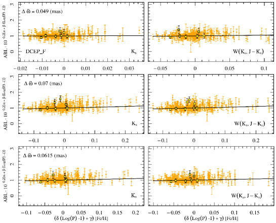
Figure 3: Same as in Fig. 2, but fitting an ABL in the general form of Eq. 5 (left panels) and Eq. 6 (right panels), for three different choices of the Gaia parallax zero point offset. The fit is presented only for fundamental mode pulsators as no sensible fit could be performed of the 10 DCEPs, due to their paucity in our sample.

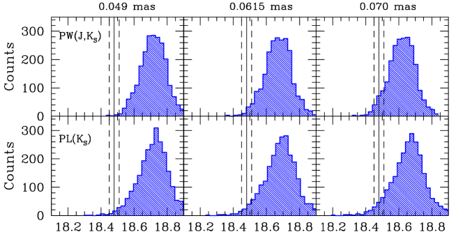
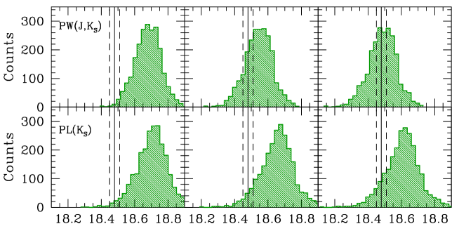
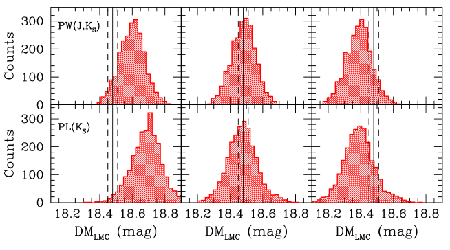
Figure 4: Distribution of the individual DMs for DCEP_Fs in the LMC based on distances calculated using: i) the ABL in the form of Eq. 1 and  2 (top panels, blue histograms); ii) the ABL in the form of Eq. 3 and  4 (middle panels, green histograms); iii) the ABL in the form of Eq. 5 and  6 (bottom paneles, red histograms) and the NIR photometry of the VMC survey (see text for details). From left to right, the different panels show results obtained for three different values of the Gaia parallax zero point offset, namely, $\Delta\varpi$=0.049, 0.0615 and 0.070 mas. A vertical solid line shows the LMC distance modulus by Pietrzyński et al. (2019), with dashed lines representing its 1 $\sigma$ uncertainty.

3 Period-Luminosity-Metallicity and Period-Wesenheit-Metallicity relations in the NIR for the Galactic DCEPs

We have used our final sample of 373 DCEP_Fs and 50 DCEP_1Os to derive a new PL relation in the $K_{S}$ band and a new PW relation in the $J,K_{S}$ bands. First, we obtained dereddened $K_{S,0}$ magnitudes needed to construct the PL${}_{K_{S}}$ relation by adopting $A_{K_{S}}=0.34E(B-V)$ ( as derived by Cardelli et al., 1989, using $R_{V}$=3.1) where the $E(B-V)$ values are those collected in Paper I. The corresponding Wesenheit magnitudes $w=Ks-0.69(J-K_{S})$ are instead reddening-free by construction.

To avoid introducing any bias or sample truncation, we did not make any selection of the DCEPs based on their parallax and/or the ratio of parallax error over parallax, hence retaining also a few objects with negative parallax. To handle also negative parallaxes we adopted the approach introduced by Feast & Catchpole (1997) and Arenou & Luri (1999), and computed the Astrometric Based Luminosity (ABL), that in the simplest case is defined as follows:

$${\rm ABL}=10^{0.2M_{K_{S,0}}}=10^{0.2[\alpha+\beta(\log P-\log P_{0})]}=\varpi 10^{0.2K_{S,0}-2}$$ (1)

$${\rm ABL}=10^{0.2W}=10^{0.2[\alpha+\beta(\log P-\log P_{0})]}=\varpi 10^{0.2w(J,K_{S})-2}$$ (2)

where $K_{S,0}$, $w(J,K_{S})$, the period P and the parallax $\varpi$ are the observables; the unknowns are the two parameters $\alpha$ and $\beta$ defining the absolute quantity $M_{abs}=\alpha+\beta(\log P-\log P_{0})$, which corresponds to the absolute magnitude $M_{K_{S,0}}$ in Eq. 1 and to the absolute Wesenheit magnitude $W(J,K_{S})$ in Eq. 2. Note the use of a pivoting (logarithmic) period $P_{0}$ of 1.0 ($P_{0}$=10 d) for DCEP_Fs and 0.3 ($P_{0}$= 2 d) for DCEP_1Os, to reduce the correlation between the parameters of the fit. The $\alpha$, $\beta$ values were calculated by a weighted least-squares fit procedure with $\sigma$-clipping of the residuals, adopting a double Median Absolute Deviation (MAD) with amplitude=4.5 MAD to limit the maximum number of rejected objects to $\sim$10%. Uncertainties were estimated through a bootstrap technique. The fit of the ABL function was carried out adopting three different values for the offset of the Gaia parallax zero point, namely, $\Delta\varpi=0.049$ mas, following Groenewegen (2018), $\Delta\varpi=0.07$ mas according to Ripepi et al. (2019) and the introduction of a third, intermediate, value: $\Delta\varpi=0.0615$ mas. The interested reader is referred to Groenewegen (2018) and Ripepi et al. (2019) for a discussion of the Gaia parallax zero point offset for DCEPs (see also Arenou et al., 2018; Lindegren et al., 2018, for a more general discussion of the topic). The results of the fitting procedure are shown in Fig. 1 where we have highlighted with different symbols the DCEPs analysed in Paper I. The coefficients of the fit of Eqs. 1 and 2 are provided in the upper portion of Table 1. We first compare our results with the PL/PW relations defined by the Large Magellanic Cloud (LMC) DCEPs, which are based on large samples, hence have very precise slopes (and intercepts). We use as a reference the PL($K_{S}$) relations by Ripepi et al. (2012) and the PW($J,K_{S}$) relations by Ripepi et al. (2020), which are based on the NIR timeseries photometry collected by the Vista Magellanic Cloud Survey (VMC Cioni et al., 2011). In particular, in the LMC these authors find PL and PW slopes of $\Delta K_{S}/\Delta\log P$=$-$3.295$\pm$0.018 and $\Delta w(J,K_{S})/\Delta\log P$=$-$3.332$\pm$0.007 for the DCEP_Fs, and $\Delta K_{S}/\Delta\log P$=$-$3.471$\pm$0.035 and $\Delta w(J,K_{S})/\Delta\log P$=$-$3.501$\pm$0.007 for the DCEP_1Os. A comparison with the values in the upper part of Table 1 allows us to make the following considerations:

• notwithstanding an increase by 12 units of the Galactic DCEP_1O sample provided by Paper I, their number is still too small to allow for precise results. Indeed, for any value of the parallax zero point offset, the slopes ($\beta$) of our MW PL and PW relations are significantly lower than for the LMC DCEP_1Os and errors are very large;

• the PL and PW relations of the MW DCEP_Fs both show meaningful slopes with reasonably small errors. For all the values of $\Delta\varpi$ such slopes appear to be significantly lower than for the LMC DCEPs. The discrepancy is at the 3$\sigma$ level for the PL relation. Since the average metallicity of the MW and LMC DCEPs differs by some $\sim 0.3-0.4$ dex, we can expect that metallicity may play a role in explaining these differences. To test this possibility, we added a metallicity term to the intercept of the PL and PW relations. In this case, the ABL formulation becomes:

  $${\rm ABL}=10^{0.2M_{K_{S,0}}}=10^{0.2\{\alpha+\beta(\log P-\log P_{0})+\gamma{\rm[Fe/H]}\}}=\varpi 10^{0.2K_{S,0}-2}$$ (3)

  $${\rm ABL}=10^{0.2W}=10^{0.2\{\alpha+\beta(\log P-\log P_{0})+\gamma{\rm[Fe/H]}\}}=\varpi 10^{0.2w(J,K_{S})-2}$$ (4)

  We adopted the same procedure as above to fit Eqs. 3 and  4 to the data, obtaining the coefficients listed in the middle portion of Table 1. Analysing these results we note that: i) for the DCEP_Fs the metallicity term is negative and generally increasingly significant as $\Delta\varpi$ increases, especially for the PW relation; for the DCEP_1Os the results seem to show the same general trend (but the dependence is positive for the PL relation). However, the errors on the slopes and intercepts of the DCEP_1O relations are up to one order of magnitude larger than for the DCEP_Fs; ii) for the DCEP_Fs, the slopes of both the PL and PW relations do not change significantly, decreasing slightly and thus becoming increasingly different than those of the LMC. The decrement is larger as the metallicity term increases, revealing an intricate inter-dependency between these parameters. In any case, it is difficult to escape the conclusion that the slopes of the PL and PW relations for the MW DCEPs differ from those of the LMC DCEPs and seem to exhibit a non-negligible metallicity dependence.
  

  More in general, our results seem to indicate that there is a complicate interplay between the metallicity dependence, due to the higher average metallicity of the MW DCEPs with respect to the LMC DCEPs, the coefficients of the PL and PW relations and the zero point offset of the Gaia parallaxes.
  In order to possibly shed light on this rather intricate scenario, we have adopted a more general form of the PL/PW relations which takes into account a metallicity dependence not only of the intercept, but also of the period coefficient. This was rendered through the following general ABL functions:

  $${\rm ABL}=10^{0.2(\alpha+(\beta+\delta{\rm[Fe/H])}(\log P-\log P_{0})+\gamma{\rm[Fe/H]})}=\varpi 10^{0.2K_{S,0}-2}$$ (5)

  $${\rm ABL}=10^{0.2(\alpha+(\beta+\delta{\rm[Fe/H])}(\log P-\log P_{0})+\gamma{\rm[Fe/H]})}=\varpi 10^{0.2w(J,K_{S})-2}$$ (6)

  which we proceeded to fit exactly in the same way as done in the previous cases, but considering only the DCEP_F pulsators, as the DCEP_1Os are too few in number to obtain meaningful results. The outcomes of this procedure are summarised in the bottom portion of Table 1 and shown in Fig. 3 (top and medium panels). We note a general behaviour similar to the previous case, with the metallicity dependence on both intercept and slope increasing as $\Delta\varpi$ increases. In no case are the metallicity terms significant for $\Delta\varpi$=0.049 mas, whereas the maximum significance is achieved for $\Delta\varpi$=0.070 mas, when both the PL and PW relations show metallicity terms significant at 1-2$\sigma$ levels. In the intermediate case $\Delta\varpi$=0.0615 mas the metallicity dependence is significant at $\sim$1$\sigma$ level. To summarise, even if the uncertainties are still rather large, and except for the PL/PW relations with $\Delta\varpi$=0.049 mas, it was possible to find a meaningful metallicity dependence for both the slope (period coefficient) and intercept. As far as we know, this is the first time that such a result is achieved, even though it still is more a qualitative than quantitative evidence. We also note that the metallicity dependence of the slope appears to have the right sign, suggesting smaller slopes as [Fe/H] increases, as inferred from the comparison of LMC and MW DCEPs and in remarkable agreement with the predictions of nonlinear convective pulsation models (see e.g. Bono et al., 1999; Marconi et al., 2005, and references therein.).

  3.1 Goodness of the fit

  In the previous part of Sect. 3 we have performed several fits of the ABL function with an increasing number of coefficients to take into account the metallicity dependence, and for different values of $\Delta\varpi$, obtaining comparable values of the ABL function residuals. Prompted by the referee, we now try to obtain an indication of the goodness of these fits. We choose to adopt the commonly used Akaike Information Criterion (AIC Akaike, 2011). For this we first need to calculate the likelihood of each of the fitted ABL functions. Therefore, we define:

  $$\ln{\mathcal{L}}=-0.5\sum_{i=1}^{N}\left[\left(\frac{res_{i}}{s_{i}}\right)^{2}+\ln(s_{i}^{2})\right]$$ (7)

  where $N$ is the number of fitted points, $res_{i}$ is the $i^{th}$ residual around the fitted relations ( Eqs. 1 to 6 above), while the term $s_{i}$ is the sum in quadrature of the $i^{th}$ uncertainty and the intrinsic scatter around the fitted relation. We have set the intrinsic scatter of the fitted relations equal to half the rms of the residuals, but checked that this choice does not affect the results significantly. The values of the likelihood can now be used to estimate the AIC quantity, which is defined as:

  $$AIC=2k-2\ln{\mathcal{L}}$$ (8)

  where k is the number of fitted parameters. The AIC values are reported in the last column of Tab. 1. By definition, the lower is the AIC value, the better is the fit. An analysis of Table 1 reveals that introducing the metallicity terms on the intercept and slope has different effects on the PL and PW relations. Specifically, the introduction of a metallicity term on the intercept of the PL relation does not improve the fit to the data significantly, whereas the inclusion of a metallicity dependence for both coefficients seems to improve the fit since, except for $\Delta\varpi$=0.049 mas, the coefficients of the PL relation become more than $\sim 1\sigma$ significant. The introduction of the metallicity term on the intercept produces an improvement of the PW relation fit. The adoption of the metallicity term also on the slope, produces a slightly better or equal goodness of the fit. The best value of the AIC is obtained for the PW relation with $\Delta\varpi$=0.070 mas.

  In summary, use of the AIC goodness of fit parameter allowed us to verify that the progressive inclusion of the metallicity term on the intercept and slope of the PL/PW relations, produces fits to the data which, except in the case of $\Delta\varpi$=0.049 mas, are generally (slightly) better than the cases when less parameters are used in the definition of the ABL function.

  4 Discussion and concluding remarks

  We can now test our PL/PW relations by applying them to the LMC DCEP_F sample in Ripepi et al. (2020) and comparing the resulting LMC distance modulus ($DM_{\rm LMC}$) to the distance to the LMC provided by the geometric determination of Pietrzyński et al. (2019): $DM_{\rm LMC}$=$18.48\pm 0.03$ mag (including systematic errors), which is currently considered one of the most accurate measure in the literature.

  We calculate the absolute $M_{K_{0,S}}$ and Wesenheit magnitudes $W(J,K_{S})$ for each LMC DCEP_F in Ripepi et al. (2020), by inserting the proper periods in the respective equations in Table 1 for the three different cases: i) with only the coefficients $\alpha$ and $\beta$; ii) with the addition of the $\gamma$ term; iii) with the further addition of the $\delta$ coefficient. In cases i) and ii) we are implicitly assuming that there is no difference in the slope (period term) of the PL/PW relations of the MW and LMC DCEPs. In cases ii) and iii) we adopted an average metallicity for the LMC DCEPs of $\langle$[Fe/H]$\rangle$=$-$0.33 dex from Romaniello et al. (2008). In all three cases, from the observed $K_{0,S}$ and $w(J,K_{S})$ we obtained individual DM values for each LMC DCEP_F. The distributions of these DMs are shown in Fig. 4 from top to bottom for the three cases i)-iii) and from left to the right for the three adopted values of $\Delta\varpi$=0.049, 0.0615 and 0.070 mas, respectively. In each panel we compared the DM distributions with the LMC geometric distance by Pietrzyński et al. (2019). In all cases the histograms show rather narrow distributions with average dispersion on the order of 0.08-0.09 mag.

  The top panels of Fig. 4 (blue histograms) show that in all cases, solution i), no metallicity dependence, provides $<DM_{\rm LMC}>$ values which are much larger than the LMC geometric distance by Pietrzyński et al. (2019). A significantly larger $\Delta\varpi$ offset would be needed to reconcile the two results. The middle panels of Fig. 4 (green histograms) corresponding to case ii) (metallicity dependence only on the intercept), still provide too large $<DM_{\rm LMC}>$ values except in the case of the PW relation with $\Delta\varpi$=0.070 mas, which, however, has the largest difference in slope with respect to the observed LMC PW relation. Finally, the bottom panels of Fig. 4 (red histograms), corresponding to case iii) (metallicity dependence of both slope and intercept) are in very good agreement with the $<DM_{\rm LMC}>$ value by Pietrzyński et al. (2019) for $\Delta\varpi$=0.0615 mas, whereas the other two values of $\Delta\varpi$ produce either lower or larger $<DM_{\rm LMC}>$ estimates.

  Therefore, the general formulation of the PL/PW relations, is not only able to qualitatively explain the different slopes of the PL/PW relations in the MW and LMC, but it also allows us to obtain an estimate of the zero point offset of the Gaia DR2 parallaxes for DCEPs. An error on the offset value can be inferred from the uncertainty on the LMC distance modulus by Pietrzyński et al. (2019). This corresponds to 0.03 mag, which translates into a 0.004 mas error in the parallax offset. Therefore, our best estimate for the Gaia DR2 zero point parallax offset for our DCEP dataset is 0.0615$\pm$0.004 mas. It is important to remark that this zero point offset has to be considered as an average valid only for the particular DCEP dataset used here, as in general, the zero point offset of the Gaia parallaxes varies for different groups of objects and different positions in the sky (see e.g. Arenou et al., 2018; Lindegren et al., 2018; Leung & Bovy, 2019).

  To conclude, the general PL/PW relations provided in the bottom part of Table 1 could represent a step forward in our ability to measure distances through DCEPs, with a potential great impact on the cosmic distance scale and the estimate of H₀. Additional spectroscopic measurements for DCEPs both in the MW and the LMC, as well as more precise parallaxes expected from the forecoming Gaia Early Data Release 3 will be fundamental to confirm the results presened in this paper.