Safe and Effective Picking Paths in Clutter
given Discrete Distributions of Object Poses

Abstract

Picking an item in the presence of other objects can be challenging as it involves occlusions and partial views. Given object models, one approach is to perform object pose estimation and use the most likely candidate pose per object to pick the target without collisions. This approach, however, ignores the uncertainty of the perception process both regarding the target’s and the surrounding objects’ poses. This work proposes first a perception process for 6D pose estimation, which returns a discrete distribution of object poses in a scene. Then, an open-loop planning pipeline is proposed to return safe and effective solutions for moving a robotic arm to pick, which (a) minimizes the probability of collision with the obstructing objects; and (b) maximizes the probability of reaching the target item. The planning framework models the challenge as a stochastic variant of the Minimum Constraint Removal (MCR) problem. The effectiveness of the methodology is verified given both simulated and real data in different scenarios. The experiments demonstrate the importance of considering the uncertainty of the perception process in terms of safe execution. The results also show that the methodology is more effective than conservative MCR approaches, which avoid all possible object poses regardless of the reported uncertainty.

I Introduction

Item picking arises in many robot manipulation applications. It involves the integration of perception and planning for recognizing the target item and then computing the motion of a robot arm for picking it. Clutter, however, can significantly complicate the challenge as it introduces occlusions and partial views. It reduces the fidelity of object recognition and introduces uncertainty, both for the target item as well as surrounding objects. One solution - given access to an RGB-D sensor - is to compute a picking path which does not collide with the point cloud. In clutter, however, considering only the visible point cloud frequently results in collisions as it does not include the back side of objects, which may be close or attached to the target item.

I-A Setup given Uncertainty in Perception

This work focuses on the case where models of objects are available but it is unknown which of these objects are present in the scene except the target item. Given object models, object recognition and 6D pose estimation algorithms allow to identify which objects are present and their poses. Many 6D pose estimation algorithms [1, 2, 3] depend on point cloud registration [4]. This process first generates pose hypotheses for the object, which are then scored on how well they align with the observed point cloud. They typically return the most likely pose hypothesis. This process, however, ignores the effects of clutter, which introduces uncertainty in pose hypothesis generation and point cloud alignment. Ambiguities arise due to occlusions as well as imperfect learning-based prior models. For instance, when training only over simulated data, which is often a necessity as it scales better over many object models.

Figure 1: Left: An RGB image for a scenario considered in this work. The target “Jell-o” object is located between and in close proximity to other objects. Center: Point cloud obtained from the RGB-D sensor highlighting the occlusions and partial object views. Right: Example output of pose estimation returning a discrete set of poses for objects in the scene.

Experiments in this paper show that using only the most likely pose estimate for each surrounding object frequently results in collisions. The idea is to consider a discrete set of pose hypotheses per object and define the likelihood for each hypothesis given how well they match with the point cloud. This gives rise to a discrete distribution of object poses. Figure 1 gives a real scene example and uses 6D pose estimation based on prior work [5] to define a discrete distribution of object poses. Then, the planning problem is to compute a path of low collision risk that attaches the arm to the target given this discrete pose distribution and the likelihood of each object being in the scene.

Figure 2: Perception pipeline developed to return the likelihood of each object existing in the scene and a discrete distribution of object poses.

I-B Relation to the Motion Planning Literature

Planning under uncertainty is often formulated as a Partially Observable Markov Decision Process (POMDP) [6], where a solution is a policy. Finding an optimal policy can be intractable [7], which motivates approximations, such as computing a plausible open-loop plan and updating it as more information is acquired [8]. Updating the scene, however, can be computationally expensive and, for the considered task, new observations do not necessarily provide additional information. This motivates open-loop planning for the safest path, which does not consider future observations, such as conformant probabilistic planning (CPP) [9]. CPP approaches have been used in robotics task such as rearrangement under uncertainty [10, 11, 12]. Recent work formalizes manipulation under uncertainty as the blindfolded robot setting [13] where the obstacles are only sensed through contact. A pick-and-place system has been designed [14] to enable manipulation on novel objects with little prior knowledge. The current paper has the objective of finding safe, open-loop solutions. It focuses on discrete distributions for the presence of collision volumes and also tackles the case where the target itself is uncertain.

A heuristic way to achieve safety is to stay sufficiently away from obstacles by growing the robot’s shape by an uncertainty bound [15]. If the obstacles’ geometry is uncertain, the area around estimated obstacles can be expanded into a shadow whose size depends on uncertainty [16]. Often the model of uncertainty assumes a continuous Gaussian probability distribution [17, 18]. Recent work computes obstacles geometric bounds with only partial shape information, assuming Gaussian distributed faces [19, 20]. There has not been much prior work, however, which focuses on discrete sets of object poses, which can be an effective way to model multi-modal distributions.

I-C Contributions

A. This paper proposes a perception pipeline to predict object existence in a scene and return the corresponding pose hypotheses with associated probabilities on top of modern 6D pose estimation algorithms [5]. It integrates this perception output with a planning approach to maximize the probability of finding collision-free and successful picking paths.

B. This paper identifies the connection between planning under discrete models of uncertainty with failure-explanation planning problems, such as Minimum Constraint Removal (MCR) problems [21, 22], which are known to be computationally hard. While typical motion planning assumes a collision-free solution can be found, tasks considered here can result in no obvious collision-free solution. For instance, if all possible object poses are avoided, then the target item is not reachable. MCR paths minimize the number of constraints to be removed to admit a constraint-free solution [22, 23, 24]. The planning challenge of this work can be seen as a stochastic version of MCR, where instead of minimizing the number of constraints, the objective is to minimize the sum of the constraints’ weights, i.e., the probabilities of the objects occupying poses along the solution path. In this way, this work promotes the use of failure-explanation planning in solving planning problems under uncertainty.

C. Experiments have been performed in simulation and with real data in different setups (table or shelf) and scenarios (clutter, narrow passage, an “arch” of objects). The experiments show the importance of considering multiple object poses in contrast to most likely pose alternatives and the benefits of the stochastic formulation of MCR proposed here, which is more effective than a conservative adaptation of MCR, which avoids all possible object poses.

II Generation of Discrete Pose Distributions

The first task is to recognize which objects are in the scene and their poses. This work utilizes the perception pipeline in Fig. 2. The workspace $\mathcal{W}$ is assumed to contain some known obstacles $\mathcal{O}_{st}$ (e.g., a table or a shelf), and can contain any of up to $N$ objects from a set $\mathcal{O}_{obj}=\{O_{1},\dots,O_{N}\}$, for which 3D models are available. There is a target item $O_{t}$ in the scene, for which a model is also available.

II-A Learning the existence probability of objects

Given an RGB image, a fully convolutional neural network (FCN) [25] is designed to detect the objects in the scene and to compute their segmentation masks. The neural network comprises a VGG16 feature encoder [26], followed by classification (lower branch in Fig. 2) and segmentation (top branch in Fig. 2). The classification outputs confidence scores corresponding to the probability $X_{i}$ of each object $O_{i}\in\mathcal{O}_{obj}$ detected in the scene. The segmentation outputs $N$ probability masks, one corresponding to each object possibly in the scene. Each pixel in an objects’ probability mask indicates the chance of the object being present at that pixel.

II-B Obtaining object pose hypotheses

Given the probability maps from the segmentation, a geometric model matching process [27] is initiated for all objects with $X_{i}$ greater than a threshold (0.3 in experiments). The process samples and evaluates a large number of pose hypotheses for each object. The poses are scored based on the point cloud matching between the observed point cloud and the object model placed at hypothesized poses. The poses are then sorted based on their matching scores and clustered. The clustering iterates over the poses in order of their scores. If a pose hypothesis is close to a higher-ranked pose (within 2.5cm and 15 degrees), it is clustered with and represented by the higher-ranked one. This ensures that similar poses are not selected and the representative is the one with highest alignment score. Finally, the top $K$ pose representatives for each object $O_{i}$ are returned with scores normalized to sum up to the existence probability, $X_{i}$. Denote $p_{i}^{j}$ as the $j$-th pose of object $O_{i}$ and $Pr(p^{j}_{i})$ as the probability that object $O_{i}$ will appear at pose $p^{j}_{i}$. Then:

$$X_{i}=\sum_{j=1}^{K}Pr(p_{i}^{j})\leq 1,\ \ \ \ \ \forall i\in[1,\dots,N].$$ (1)

The target item is assumed to be in the scene, i.e., $X_{t}=1$. There is uncertainty, however, regarding its poses as well, i.e., poses $p_{t}^{j}$ with probabilities $Pr(p_{t}^{j})$ are also detected for it. The number of hypotheses $K$ for each object can vary. For simplicity, the same value is used for all objects.

III Problem setup and notation

Path Robustness. The robustness of a path in this paper is defined based on two aspects:

1) Minimum collision probability with objects: The scene will be re-sensed and replanning is performed if a collision occurs. Thus, a path with minimum collision probability reduces overall execution time to complete a task.

2) Maximum probability of reaching the target item: Since the target $O_{t}$ also carries uncertainty, a safe path may end up having low probability to pick the object, which necessitates replanning. Therefore, maximizing the probability of reaching the target object is also important for task completion.

Definition 1.

($C$-space): The configuration space ($C$-space) $\mathbb{C}$ of the robot arm is the set of all arm configurations. $\mathbb{C}_{p}$ is defined as the set of arm configurations, which end up in collision with an object pose $p$.

Definition 2.

(Goal configurations): $\mathbb{Q}_{goal}$ is a set of configurations where the arm can pick the target object at poses $p_{t}^{j}$. $\mathcal{T}=[1,\dots,K]$ is the set of indices of all $K$ target poses. Each goal configuration $q_{g}\in\mathbb{Q}_{goal}$ is associated with a set $J(q_{g})\subseteq\mathcal{T}$ indicating which target poses $q_{g}$ can pick. Then, the probability that a path $\pi$ from the initial configuration $q_{s}$ to any goal configuration $q_{g}$ leads to a successful picking of $O_{t}$ is $Pr(q_{g})=\sum_{j\in J(q_{g})}Pr(P_{t}^{j})$, i.e., equal to the probability that the target $O_{t}$ is at one of the poses $q_{g}$ can pick.

Definition 3.

(Survivability of a path) A path $\pi:[0,1]\rightarrow\mathbb{C},\pi(0)=q_{s},\pi(1)\in\mathbb{Q}_{goal}$ survives an object $O_{i}$, if it does not collide with $O_{i}$. The survivability of a path $\pi$, denoted as $S_{\pi}$, is the probability that $\pi$ survives all the objects.

Define $E_{i}$ as the event that $\pi$ collides with object $O_{i}$ and $\overline{E_{i}}$ its complementary event. Then, $E_{i}^{j}$ is defined as the event that $\pi$ collides with object $O_{i}$ when $O_{i}$ is at pose $p_{i}^{j}$. Then $E_{i}=\bigcup_{j=1}^{K}E_{i}^{j}$. The events that $O_{i}$ appears at different candidate poses are mutually exclusive, which indicates mutual exclusiveness of $E_{i}^{j}$. Thus, the probability that $\pi$ does not collide with $O_{i}$ is:

$$Pr(\overline{E_{i}})=1-Pr(E_{i})=1-Pr(\bigcup_{j=1}^{K}E_{i}^{j})=1-\sum_{j=1}^{K}Pr(E_{i}^{j}).$$ (2)

Then, the survivability of a path for all objects $O_{i}\in\mathcal{O}_{obj}(i=1,\dots,N)$ is computed as:

$$S_{\pi}=Pr(\bigcap_{i=1}^{N}\overline{E_{i}})=\prod_{i=1}^{N}Pr(\overline{E_{i}})=\prod_{i=1}^{N}(1-\sum_{j=1}^{K}Pr(E_{i}^{j})).$$ (3)

$S_{\pi}$ represents the first aspect of path robustness, i.e., minimum collision probability with objects. The higher $S_{\pi}$ is, the less risky the path is in terms of collision.

Definition 4.

(Success probability): Define $E$ as the event that the path survives all objects and $F$ as the event that the robot arm reaches the target item. Both events E and F must occur for a path $\pi:q_{s}\rightarrow q_{g}$ to successfully reach the target. Define the success probability of a path to be $Succ(\pi)=Pr(E,F)$. Then, $Succ(\pi)$ can be rewritten as:

$$Succ(\pi)=Pr(E,F)=Pr(E)\cdot Pr(F)=S_{\pi}\cdot Pr(q_{g}|\pi).$$ (4)

The events $E$ and $F$ are independent with one exception, which leads to defining $Pr(F)=Pr(q_{g}|\pi)$. When a path leading to a goal $q_{g}$ collides with the target pose $p_{t}^{j}$ with which $q_{g}$ is associated, $q_{g}$ is no longer considered for the path as a valid goal configuration for $p_{t}^{j}$, since: (1) if the target item $O_{t}$ is at pose $p_{t}^{j}$, the path will be in collision with $O_{t}$ or (2) if the target item $O_{t}$ is not at pose $p_{t}^{j}$, then $q_{g}$ does not allow picking $O_{t}$ at pose $p_{t}^{j}$.

This means that $Pr(q_{g})$ should be conditioned on the path. Define ${\overline{J}}_{\pi}$ as the target poses intersected by the path. Then, the remaining valid target poses for $q_{g}$ should be $\hat{J}_{\pi}(q_{g})=J(q_{g})\setminus{\overline{J}}_{\pi}$ and $Pr(q_{g}|\pi)$ is set to be:

$$Pr(q_{g}|\pi)=\sum_{j\in\hat{J}_{\pi}(q_{g})}Pr(P_{t}^{j}).$$ (5)

Define the path space $\Pi$, which includes the set of candidate paths $\pi:q_{s}\rightarrow q_{g}$, where $q_{g}\in\mathbb{Q}_{goal})$. The overall objective is to find a path $\pi^{*}$:

$$\pi^{*}=\operatorname*{arg\,max}_{\pi\in\Pi}Succ(\pi).$$ (6)

IV Algorithmic Framework

Consider a roadmap $G(V,E)$, where $q\in V$ corresponds to an arm configuration and $e\in E$ the transition between two arm configurations. If an edge $e$ connecting $q_{1}$ and $q_{2}$ intersects with a pose $p^{j}_{i}$, a label $l^{j}_{i}$ is assigned to that edge and the weight for the label $w(l^{j}_{i})=Pr(p^{j}_{i})$.

The survivability $S_{\pi}$ depends on the probability that the objects will appear at any pose that the path intersects. So $Pr(E^{j}_{i})$ in Eq.3 depends on whether there is an edge $e$ along the path $\pi$ that has a label $l_{i}^{j}$. If such an edge exists along the path, then $Pr(E_{i}^{j})=Pr(p_{i}^{j})=w(l_{i}^{j})$. Otherwise, $Pr(E_{i}^{j})=0$. An indicator random variable $\mathds{1}_{\pi}(j,i)$ for each pose $j$ of each object $i$ is defined as

$$\mathds{1}_{\pi}(j,i)=\begin{cases}1,&\text{if}\ \pi\ \text{carries label}\ l_{i}^{j}\\ 0,&\text{otherwise}.\end{cases}$$ (7)

Then $S_{\pi}$ in a labeled roadmap can be computed as

$$S_{\pi}=\prod_{i=1}^{N}(1-\sum_{j=1}^{K}Pr(E_{i}^{j}))=\prod_{i=1}^{N}(1-\sum_{j=1}^{K}w(l_{i}^{j})\mathds{1}_{\pi}(j,i)).$$ (8)

Eq. 8 computes $S_{\pi}$ for a path from $q_{s}$ to any currently examined state $q_{curr}$ by checking the labels $L_{q_{curr}}$ the path $\pi:q_{s}\rightarrow q_{curr}$ carries. To compute the prospect of the path $\pi$ accurately reaching the target, two situations are considered:

(i) If $q_{curr}$ is a goal configuration $q_{g}$, the probability that the path leads to the goal is computed according to Eq. 5.

(ii) If $q_{curr}\notin{Q}_{goal}$, the path is not complete and $T_{q_{curr}}\subseteq\mathcal{T}$ indicates the indices of remaining target poses the path $\pi:q_{s}\rightarrow q_{curr}$ can reach. If the current path $\pi:q_{s}\rightarrow q_{curr}$ carries a label $l_{t}^{j}$, then the path and its extensions can no longer treat $p_{t}^{j}$ as a valid target pose. In this case, $T_{q_{curr}}$ is updated by removing pose index $j$ from $T_{q_{curr}}$. An example is given in Fig. 3(left). Then the probability for the current path $\pi:q_{s}\rightarrow q_{curr}$ leading to the true target will be

$$Pr(q_{curr}|\pi)=\sum_{j\in(T_{q_{curr}}\setminus{\overline{J}}_{\pi})}Pr(p_{t}^{j})$$ (9)

Figure 3: (Left) A path $\pi:q_{s}\rightarrow q_{curr}$ intersects pose $p_{t}^{1}$, which makes $q_{g^{1}}$ no longer valid for this path. The remaining goals will be $\{q_{g^{2}},q_{g^{3}}\}$ and $T_{q_{curr}}=[2,3]$ (Right) The goal $q^{\prime}_{g^{1}}$ is not available since the path from $q_{curr}$ to $q^{\prime}_{g^{1}}$ collides with pose $p_{t}^{1}$. But it is still available if being reached via $q_{n}$. $q_{g^{1}}$ can also be treated as an intermediate configuration to reach a potentially more promising goal $q_{g^{2}}$. The child node for the path ending at $q_{g^{1}}$ will be added to search twice, once as a goal node, once as a non-goal node.

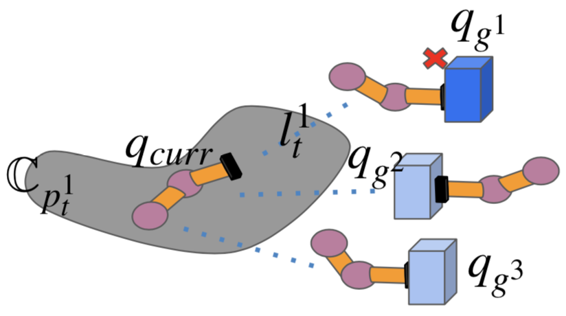
With Eq. 5, 8 and 9, the success probability $Succ(\pi)$ of a path $\pi:q_{s}\rightarrow q_{curr}$ can be computed, which is used as the objective function during the search.

IV-A Challenge - Lack of Optimal Substructure

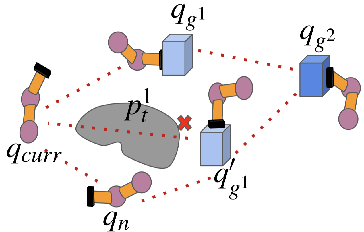
Consider the setup in Fig. 4(left) where the locally optimal path is not globally optimal, i.e., the search algorithm cannot just remember the locally optimal path (greedy search). For the related MCR problem, it has been argued that greedy search (where only the best local path is stored at each node) still guarantees an optimal solution if the optimal path encounters each obstacle once [22]. Even with this assumption for the current problem, greedy search still has a chance of failing to find the optimum (Fig. 4(right)). A straightforward reduction of the problem to the computationally hard MCR problem can be found in the Appendix.

Figure 4: (Left) There are 2 poses $Pr(p_{1})=0.3$ and $Pr(p_{2})=0.4$. Two paths are considered: the pink path $q_{s}\rightarrow q_{a}\rightarrow q_{m}$ is favored vs. the blue one $q_{s}\rightarrow q_{b}\rightarrow q_{m}$ locally as it has a lower collision probability. Nevertheless, both paths go through pose $p_{2}$ afterwards ($q_{m}\rightarrow q_{g}$). Thus, the optimal path to $q_{g}$ is actually the blue one, which only collides with pose $p_{2}$ with probability 0.4. (Right) There are 3 poses: $p_{1}^{1}$ and $p_{1}^{2}$ for object $O_{1}$ with $Pr(p_{1}^{1})=0.3$ and $Pr(p_{1}^{2})=0.3$, while $p_{2}^{1}$ belongs to $O_{2}$ with $Pr(p_{2}^{1})=0.4$. Again the pink path $q_{s}\rightarrow q_{a}\rightarrow q_{m}$ is locally favored since it has higher survivability $1-Pr(p_{1}^{1})=0.7$ than that of the blue path $q_{s}\rightarrow q_{b}\rightarrow q_{m}$ ($1-Pr(p_{2}^{1})=0.6$). But when both paths reach $q_{g}$, the pink path has survivability $1-Pr(p_{1}^{1})-Pr(p_{1}^{2})=0.4$, which is lower than that of the blue path $(1-Pr(p_{2}^{1}))(1-Pr(p_{1}^{2}))=0.42$.

IV-B MaxSuccess Search

Since greedy search is not guaranteed to be optimal, a complete search method is proposed here, which follows the exact search for the MCR problem but adapts it to address the survivability objective defined here. The algorithm stores a path to a node only if the label set of the path is not a superset of that of any path found reaching the same node. It theoretically guarantees optimality since a path with a superset of labels cannot have a higher $Succ(\pi)$ value than that of a path reaching the same node with a subset of labels.

Input: $G(V,E),q_{s},\mathbb{Q}_{goal},\mathcal{T}=[1,\dots,K]$

Output: $\pi^{*}$

1 $Q\leftarrow\text{{\sc Add}}(q_{s},L_{q_{s}}=\emptyset,T_{q_{s}}=\mathcal{T},\mathds{1}_{q_{s}}=false)$

2 while goal not found do

3       $q_{curr}\leftarrow Q.top()$

4       if $\mathds{1}_{q_{curr}}=true$ then

5             return $\pi:q_{s}\rightarrow q_{curr}$

6      for $\text{each }q_{neigh}\in\text{Adj}(G,q_{curr})$ do

7             $L_{q_{neigh}}=L_{q_{curr}}\cup L_{e}(q_{curr},q_{neigh})$

8             if $\text{not }\textsc{IsSuperSet}(L_{q_{neigh}})$ then

9                   $q_{neigh}.{\pi}\leftarrow q_{curr}.{\pi}\cup e(q_{neigh},q_{curr})$

10                   $S_{q_{neigh}.{\pi}}\leftarrow\textsc{GetSurvival}(L_{q_{neigh}})$

11                   $T_{q_{neigh}}\leftarrow\textsc{UpdateGoals}(L_{q_{neigh}})$

12                   $Pr(q_{neigh}|\pi)\leftarrow\textsc{GetReach}(T_{q_{neigh}})$

13                   $Succ(q_{neigh}.{\pi})\leftarrow S_{q_{neigh}.{\pi}}\cdot Pr(q_{neigh}|\pi)$

14                   $Q\leftarrow\text{{\sc Add}}(q_{neigh},L_{q_{neigh}},T_{q_{neigh}},false)$

15                   if $q_{neigh}\in\mathbb{Q}_{goal}$ then

16                         if $\text{{\sc IsValid}}(q_{neigh},T_{q_{neigh}})$ then

17                               $Q\leftarrow\textsc{Add}(q_{neigh},L_{q_{neigh}},T_{q_{neigh}},true)$

Algorithm 1 MaxSuccess Exact Search

Table 1 (narrow passage)	Table 2 (clutter)	Shelf 1 (narrow passage)	Shelf 2 (clutter)

Figure 5: Results on 4 tests (2 for tabletop and 2 for shelf) evaluating the number of objects collided for (top) different number of pose hypotheses under uncertainty level 4 and (middle) different uncertainty levels for 4 poses per object. Each column corresponds to the benchmark shown below it. The target object is the baseball in the tabletop and the water bottle in the shelf. The dots are average values and the background color indicates variance.

The method is outlined in Alg. 1. It receives as input the roadmap $G(V,E)$, the start arm configuration $q_{s}$, a set of goal configurations $\mathbb{Q}_{goal}$ and a list of all target poses indices $\mathcal{T}$. A priority queue $Q$ (line 1) prioritizes nodes with higher $Succ(\pi:q_{s}\rightarrow q)$. Each state $q$ is specified with a label set $L_{q}$ indicating the labels the path $\pi:q_{s}\rightarrow q$ carries and the set of indices of the target poses $T_{q}\subseteq\mathcal{T}$ the path $\pi$ can reach. An indicator $\mathds{1}_{q}$ is assigned to a node to indicate whether it is a goal. If it is a goal, then it is found with the highest $Succ()$ (line 4-5). If not, it computes the labels that the path from $q_{s}$ to all adjacent nodes $q_{neigh}$ via $q_{curr}$ carries (line 6-7). If the set of labels is not a superset of that of any previously stored paths $\pi:q_{s}\rightarrow q_{neigh}$ (line 8), the path $\pi:q_{s}\rightarrow q_{curr}\rightarrow q_{neigh}$ is stored, with corresponding $S_{\pi}$ and $T_{q_{neigh}}$ computed (line 9-11). The probability for the path to reach the target is computed in line 12 using Eq. 9 and $Succ()$ value of the path can be computed (line 13). The node is then added to $Q$ as a non-goal node ($\mathds{1}_{q}=false$) (line 14). Then the algorithm checks if it is a goal node and whether the path $\pi:q_{s}\rightarrow q_{curr}\rightarrow q_{neigh}$ still treats this goal $q_{neigh}$ as a valid one (line 15-16). If $q_{curr}$ meets both conditions, it is added to $Q$ as a goal ($\mathds{1}_{q}=true$) (line 17). The search terminates when a goal $q_{g}\in\mathbb{Q}_{goal}$ has been found (line 5) or there is no solution.

A key observation is that each node has a chance to be added to $Q$ twice in a single iteration (line 14 and line 17). If it is a non-goal node, it will only be added once (line 14). A goal node can be treated as a goal configuration to grasp an object, but it can also be treated as an intermediate node to reach a more promising goal configuration. For that reason, the node is added as a non-goal node (line 14) as usual. Then, the node is only added as a goal node (line 17) if it is still valid (Fig. 3(right)).

V Experimental Evaluation

The proposed planning framework in IV is evaluated on (A) simulated sensing data and (B) data from a real-world setup. The following alternatives are also considered:

1. an $\tt Optimistic\ Shortest\ Path$ ($\tt OSP$) planner - which ignores the presence of the movable objects $\mathcal{O}_{obj}$,

2. an $\tt MCR$ search (Exact and Greedy) - which aims to minimize the number of collisions with all poses, and

3. an $\tt MCR\ Most\ Likely\ Candidate\ (MCR-MLC)$ search, which considers only the most likely pose for each object and aims to minimize the number of collisions.

The methods are evaluated on two robot manipulators (1) a 7-DoF Kuka LBR iiwa14 and (2) a 7-DoF Yaskawa Motoman SDA10F, each of which with a suction-based gripper. The evaluation metrics used here are (1) the number of objects colliding in the ground truth scene and (2) success rate in reaching the true target.

V-A Simulations

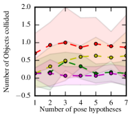
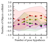
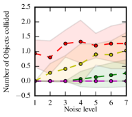
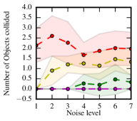
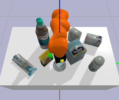
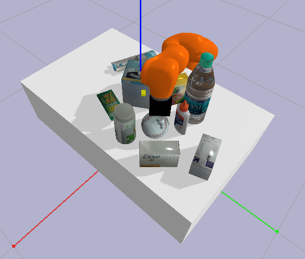
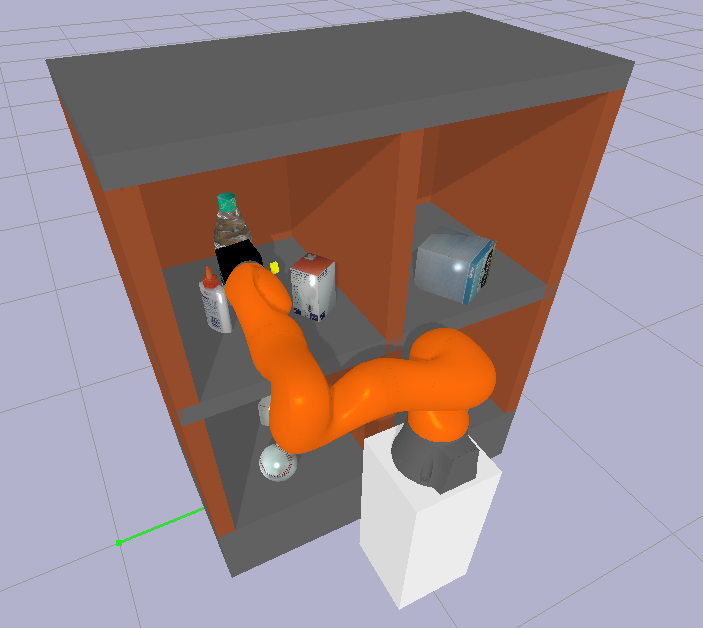
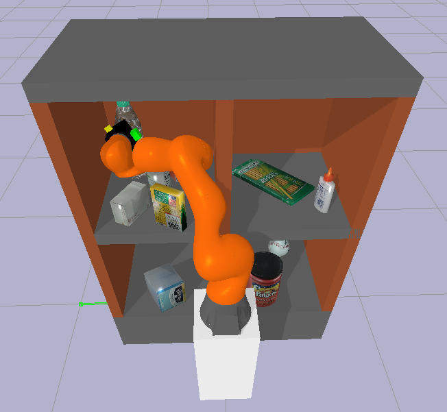
Large-scale experiments with simulated sensing data are performed first to evaluate the algorithms with different levels of uncertainty. Four benchmarks are created (Fig. 5 bottom), where benchmarks 1-2 are tabletop scenarios while benchmarks 3-4 are highly-constrained shelf scenarios. The target object is either placed in a narrow passage or in clutter.

Figure 6: Success rate for different algorithms in all 4 benchmarks.

Figure 7: Experimental results on real vision system in 3 scenarios (1) target in objects clutter (top row) (2) target in narrow passage (middle row) (3) target in front of objects arch (bottom row). The second and third column demonstrate the number of objects collided during path execution and the success rate of reaching the target, respectively, as the evaluation metrics for 6 methods (including both exact and greedy version of MaxSuccess and MCR).

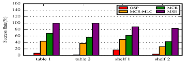
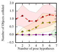
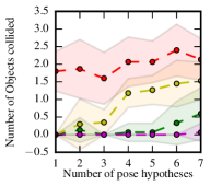
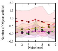
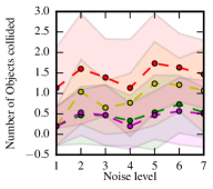
Pose hypotheses (sampled between 1-7) are generated according to probability distributions centered at the ground truth pose. Different levels of uncertainty are defined (Level 1: $\pm 0.5$ cm for translation error and $\pm 5$ degrees for orientation error; level 7: $\pm 3.5$ cm and $\pm 35$ degrees noise). Intermediate levels (2-6) are linearly interpolated between levels 1 and 7. The pose probability is assigned based on its distance from ground truth. 35 roadmaps are generated for each ground truth using a Probabilistic Roadmap (PRM) [28]. The details of the roadmap generation are provided in the Appendix. Fig. 5 provides the number of objects collided during path execution under different uncertainty.

In the tabletop benchmarks, the $\tt OSP$ paths collide with $1.54$ objects on average and $\tt MCR-MLC$ with $0.74$. In contrast, both $\tt MCR$ and $\tt MSE$ work well with much fewer collisions. As the uncertainty increases, the number of collisions for ${\tt MCR}$ methods start to increase, while the $\tt MSE$ algorithm remains almost down to zero collisions. Overall, $\tt MCR$ and $\tt MSE$ result in few collisions but Fig. 6 shows that $\tt MCR$’s success rate is not as high (68.4% for table 1 and 56.2% for table 2), since it does not reason about target uncertainty. As a result, $\tt MCR$ may avoid collisions but does not lead to the true target. Since the $\tt MSE$ methods take both safety and goal reachability to form the success function $Succ(\pi)$, the corresponding success rate is high on the tabletop scenes ($99.5\%$).

The shelf benchmarks are more challenging, as the objects must be reached from the side in a limited space, which increases the collision risk. Despite that, $\tt MCR$ and $\tt MSE$ remain safe ($0.34$ and $0.22$ collisions, respectively). Again, the $\tt MCR$ method is conservative in terms of collisions at the expense of failing to reach the true target pose. In Fig. 6, the success rate for $\tt MCR$ drops to ($42.6\%$) in benchmark 4 (clutter, shelf), while $\tt MSE$ is still able to succeed $83.6\%$ of the trials.

V-B Real-world Experiments

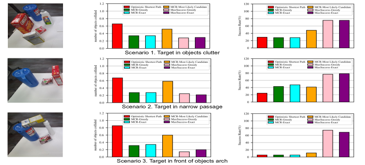
After verifying the effectiveness of the proposed $\tt MaxSuccess$ algorithm with simulated sensing data, an evaluation with real data took place. Fig. 8 shows the sensing setup used. An Azure Kinetic camera is mounted on top of a humanoid Motoman SDA10F robot to enable an overhead view of the objects on the table. The experiment focuses on overhand picks in a tabletop setup. 33 images have been taken from the camera with diverse scenarios:

Figure 8: Real system setup

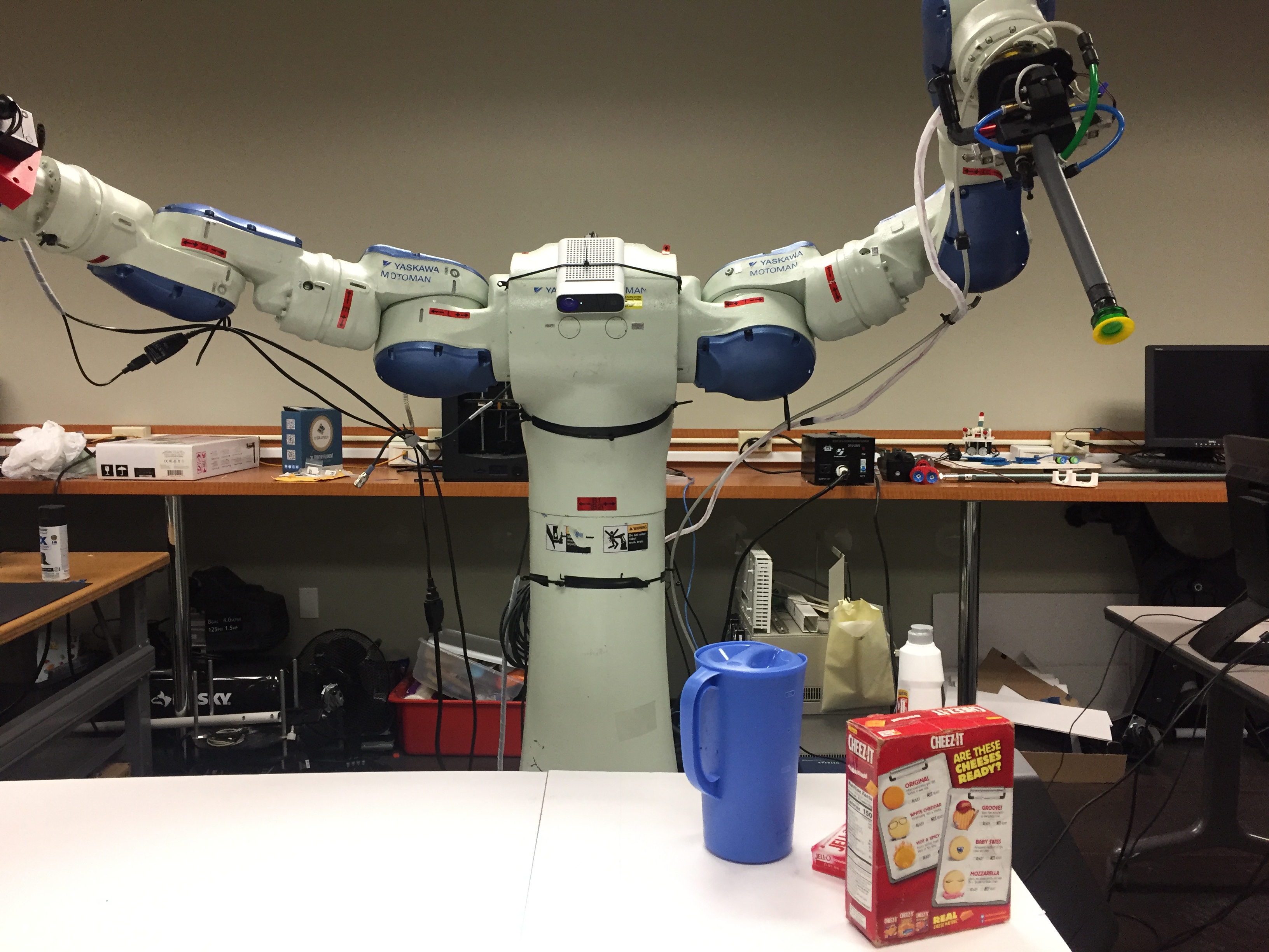
(1) target in clutter - Target surrounded by multiple objects. The robot has to reason about the objects’ uncertainty to reach the target without collision. (2) target in narrow passage - Target placed between 2 or 3 tall objects to create a narrow passage. The arm has to reach deep to pick the target. (3) target under an obstacle arch - An arch is created by three objects, where an object is put on top of the other two. The target is placed a little bit ahead of the arch. The robot is reaching the target with overhand picks, so the relative location of the arch to the target has to be carefully examined to succeed.

10 YCB objects are selected and the ”pudding box”, ”gelatin box” and ”meat can” are selected as the target in different scenes. All images went through the perception pipeline as in Section II. An object is treated as present if the probability prediction is over 0.3. Given this threshold, the accuracy of object recognition is analyzed in the Appendix. For each detected object, $K=5$ object poses have been returned with corresponding probabilities as the outcome of pose estimation and pose clustering.

The proposed planner takes these poses as input. The process generates 5 roadmaps for each scene to produce the picking paths for each method. The paths are then executed in simulation using ground truth poses to evaluate their performance. The same metrics are used: (1) number of colliding objects; and (2) success rate of reaching the target.

Figure 9: Left image shows the grasping configuration chosen by the $\tt MCR$ method. It avoids any risk of colliding with the arch but has a large chance to miss the target. The right one shows the grasping configuration chosen by $\tt MaxSuccess$. It reasons about the uncertainty of the sugar box and the target pudding box together and comes up with a better solution which can reach the target accurately with low risk of collisions.

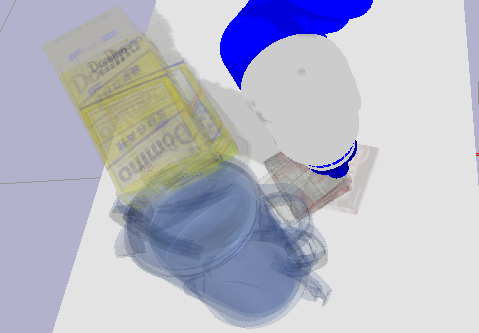
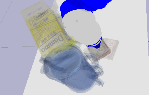
Fig. 7 demonstrates the performance of different methods with real vision data. As the scenarios have no obvious risk-free picking path, $\tt OSP$ suffers from many collisions. $\tt MCR-MLC$ also has a relatively high number of collisions, which confirms that the distribution of object poses have to be considered instead of only the most likely pose. The true pose for an object may not be the top response of pose estimation. In every scenario, the methods $\tt MSE$ and $\tt MSG$ outperform $\tt MCR-G$ and $\tt MCR-E$, which are good at finding safe paths but have low success rate of reaching the target. The $\tt MCR$ methods tend to find conservative paths to avoid obstacles, sacrificing the reasoning about target poses. This observation is highlighted in the arch scenario (Fig. 7, bottom-right bar graph). Fig. 9 shows the advantage of the proposed method over $\tt MCR$ in the arch scenarios.

VI Discussion and Future Work

This paper tackles the problem of picking a target item in the presence of multiple objects, where there is uncertainty for both obstructing objects and the target item. Perception and planning pipelines have been proposed to address this challenge. Both simulated and real-world experiments demonstrate effectiveness of the proposed framework, which minimizes collision probability while maximizing the probability of reaching the target. An interesting direction to extend this work is safe object retraction, as well as potentially clearing an entire bin of objects with uncertain poses, where the robot also needs to decide the order with which to reach the target items. A computational improvement can be achieved by reducing the overhead of collision checking as the number of pose hypotheses increases. One heuristic is to delay the collision checking [29] before finding a plausible path and check afterwards to save computation. An important extension is to deal with unknown objects or scenarios where object models are not available. In such cases a perception system can predict a volumetric representation for the objects’ poses and shape uncertainty [30], which can be incorporated into the proposed planning framework.

Appendix

VI-A Reduction from MCR to stochastic MCR

The hardness of stochastic MCR can be deduced via a reduction from MCR, the hardness of which has been shown by polynomial-time reduction from SET-COVER [22].

For MCR, the input corresponds to an initial state $q_{s}$, the goal state $q_{g}$ and $N$ objects $\mathcal{O}_{obj}=\{O_{1},\dots,O_{N}\}$. For the reduction, given any instance of MCR, the input to a corresponding stochastic MCR instance is generated according to the following polynomial-time process:

(i) the start $q_{s}$ and the goal $q_{g}$ remain the same as in MCR;

(ii) for each object $O_{i}$, the pose $P_{i}$ for object $O_{i}$ (deterministic) in MCR defines a single pose $p_{i}^{1}$ in stochastic MCR. For the target, $p_{t}^{1}$ is the only target pose for stochastic MCR and as a consequence, the target pose the goal configuration can pick is $J(q_{g})=\mathcal{T}=[1]$. Here $q_{g}$ in MCR is equivalent to a single goal $g_{g}^{1}\in\mathcal{G}$ in stochastic MCR;

(iii) all poses $p_{i}^{1}(i=1,\cdots,N)$ are assigned the same probability $\xi$, i.e., $Pr(p_{i}^{1})=\xi\ (0\leq\xi\leq 1)$.

Suppose the stochastic MCR solver is able to find a solution path $\pi^{*}$ of maximum $Succ(\pi^{*})$ value (Eq. 6) with $m$ poses intersected ($m\leq N$). In this case, $\mathds{1}_{\pi^{*}}(1,i)=1$ for those $m$ intersected poses and $\mathds{1}_{\pi^{*}}(1,i)=0$ for the remaining $N-m$ poses (Eq. 7). Then according to Eq. 8 where $j=1$, survivability $S_{\pi^{*}}$ is

$$S_{\pi^{*}}=\prod_{i=1}^{N}(1-w(l_{i}^{1})\mathds{1}_{\pi^{*}}(1,i))=(1-\xi)^{m}$$ (10)

For the term $Pr(q_{g}|\pi^{*})$, there are two cases

1. The path $\pi^{*}$ intersects the target pose $p_{t}^{1}$.

   In this case, $\hat{J}_{\pi^{*}}(q_{g})=J(q_{g})\setminus{\overline{J}}_{\pi^{*}}=\emptyset$, which indicates that there are no remaining valid poses. According to Eq. 5, $Pr(q_{g}|\pi^{*})=0$. Then $Succ(\pi^{*})=S_{\pi^{*}}\cdot Pr(q_{g}|\pi^{*})=0$, which indicates that the stochastic MCR instance is not solvable. This also indicates no solution in original MCR problem as the robot cannot grasp the target object $O_{t}$ while colliding with it.

2. The path $\pi^{*}$ does not intersect the target pose $p_{t}^{1}$.

   In this case, $\hat{J}_{\pi^{*}}(q_{g})$ remains the same since $p_{t}^{1}$ is still available and $Pr(q_{g}|\pi^{*})=Pr(p_{t}^{1})=\xi$. Then $Succ(\pi^{*})=S_{\pi^{*}}\cdot Pr(q_{g}|\pi^{*})=(1-\xi)^{m}\xi$. To maximize the quantity $(1-\xi)^{m}\xi$, parameter $m$ needs to be minimized when $\xi$ is fixed, which corresponds to the objective of original MCR problem (minimize the number of constraints violated).

Figure 10: Diagram for the reduction from MCR to stochastic MCR

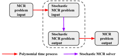
As a result, reconstructing the MCR solution from the stochastic MCR one takes polynomial time. Since the input/output transforms take polynomial time (Fig. 10), if the stochastic MCR solver can return a solution in polynomial time, then MCR is in P. Nevertheless, MCR is NP-hard [22]. Consequently, stochastic MCR is an NP-hard problem.

VI-B Roadmap generation

The roadmap is generated as the input for the planning pipeline in this paper. Here the connectivity of the roadmap is defined similar to the (PRM^∗) variant, which achieves asymptotic optimality [31], i.e., each node is connected to at least $k^{*}=k_{n}\cdot log(n)=e(1+1/d)log(n)$ neighbors, where $e$ is the base of the natural logarithm, $d$ the dimension of the search space (d=7) and $n$ the number of samples (n=5000).

VI-C Accuracy of objects recognition

As described in Section II, one branch for the perception pipeline is to output the probability of each object detected in the scene. In the real-world experiment, the objects with probability $X_{i}$ larger than 0.3 are considered as existent in the scene. Table 1 shows the statistics of the object recognition process as a confusion matrix.

	Actually exist	Actually not exist
Predict as existent	150	5
Predict as not existent	3	222
Table 1: Confusion matrix for object recognition.

Based on Table 1, precision and recall are computed as

$$\text{precision}=150/(150+5)=96.8\%$$ (11)

$$\text{recall}=150/(150+3)=98.0\%$$ (12)

The high precision ($96.8\%$) demonstrates the accuracy of excluding phantom objects (prevent extreme conservative plans) while the high recall ($98.0\%$) indicates the accuracy of detecting objects which are truly in the scene (critical for safe operation of the robot).

VI-D Path cost and planning time

The path cost (Euclidean distance between arm configurations along the path) and the planning time have also been computed for reference in Table 2, though they are not the main objectives considered in this paper.

	OSP	MCR-G	MCR-E	MLC	MSG	MSE
cost	3.023	3.627	3.705	3.255	4.221	4.425
time(s)	0.030	0.031	0.033	0.031	0.045	0.046
Table 2: Path cost and planning time.

References

- [1] V. Narayanan and M. Likhachev, “Deliberative object pose estimation in clutter,” in ICRA 2017.
- [2] C. Mitash, A. Boularias, and K. E. Bekris, “Improving 6d pose estimation of objects in clutter via physics-aware monte carlo tree search,” in ICRA 2018, Brisbane, Australia.
- [3] Y. Xiang, T. Schmidt, V. Narayanan, and D. Fox, “Posecnn: A convolutional neural network for 6d object pose estimation in cluttered scenes,” in RSS 2018, Pittsburgh, Pennsylvania.
- [4] N. Mellado, D. Aiger, and N. J. Mitra, “Super4PCS Fast Global Pointcloud via Smart Indexing,” in Computer Graphics Forum, vol. 33, 2014, pp. 205–215.
- [5] C. Mitash, A. Boularias, and K. Bekris, “Physics-based scene-level reasoning for object pose estimation in clutter,” International Journal of Robotics Research (IJRR), 2019.
- [6] L. P. Kaelbling, M. L. Littman, and A. R. Cassandra, “Planning and Acting in Partially Observable Stochastic Domains,” in Artificial Intelligence, 1998.
- [7] C. H. Papadimitriou and J. N. Tsitsiklis, “The complexity of markov decision processes,” Mathematics of operations research, vol. 12, no. 3, pp. 441–450, 1987.
- [8] R. Platt, R. Tedrake, L. P. Kaelbling, and T. Lozano-Pérez, “Belief space planning assuming maximum likelihood observations,” in Robotics: Science and Systems, 2010.
- [9] R. Taig and R. I. Brafman, “Compiling Conformant Probabilistic Planning Problems into Classical Planning,” in ICAPS 2013.
- [10] M. R. Dogar and S. S. Srinivasa, “A planning framework for non-prehensile manipulation under clutter and uncertainty,” Autonomous Robots, vol. 33, no. 3, pp. 217–236, 2012.
- [11] M. C. Koval, J. E. King, N. S. Pollard, and S. S. Srinivasa, “Robust trajectory selection for rearrangement planning as a multi-armed bandit problem,” in IROS 2015. IEEE, pp. 2678–2685.
- [12] A. S. Anders, L. P. Kaelbling, and T. Lozano-Perez, “Reliably arranging objects in uncertain domains,” in ICRA 2018.
- [13] B. Saund, S. Choudhury, S. Srinivasa, and D. Berenson, “The blindfolded robot: A bayesian approach to planning with contact feedback,” in International Symposium on Robotics Research (ISRR), 2019.
- [14] A. Zeng, S. Song, K.-T. Yu, E. Donlon, F. R. Hogan, M. Bauza, D. Ma, O. Taylor, M. Liu, E. Romo, et al., “Robotic pick-and-place of novel objects in clutter with multi-affordance grasping and cross-domain image matching,” in ICRA 2018. IEEE.
- [15] A. Bry and N. Roy, “Rapidly-exploring random belief trees for motion planning under uncertainty,” in ICRA 2011.
- [16] A. Lee, Y. Duan, S. Patil, J. Schulman, Z. McCarthy, J. Van Den Berg, K. Goldberg, and P. Abbeel, “Sigma hulls for gaussian belief space planning for imprecise articulated robots amid obstacles,” in IROS 2013. IEEE, pp. 5660–5667.
- [17] J. S. Park, C. Park, and D. Manocha, “Efficient Probalistic Collision Detection for Non-Convex Shapes,” in CoRR, 2016.
- [18] W. Sun, L. G. Torres, J. van den Berg, and R. Alterovitz, “Safe Motion Planning for Imprecise Robotic Manipulators by Minimizing Probability of Collision,” in IJRR 2016.
- [19] B. Axelrod, L. P. Kaelbling, and T. Lozano-Pérez, “Provably safe robot navigation with obstacle uncertainty,” The International Journal of Robotics Research, vol. 37, no. 13-14, pp. 1760–1774, 2018.
- [20] L. Shimanuki and B. Axelrod, “Hardness of 3d motion planning under obstacle uncertainty,” WAFR 2018.
- [21] K. K. Hauser, “Minimum constraint displacement motion planning.” in Robotics: Science and Systems, 2013.
- [22] K. Hauser, “The minimum constraint removal problem with three robotics applications,” The International Journal of Robotics Research, vol. 33, no. 1, pp. 5–17, 2014.
- [23] L. H. Erickson and S. M. LaValle, “A Simple, but NP-Hard Motion Planning Problem,” in AAAI 2013.
- [24] A. Krontiris and K. Bekris, “Computational tradeoffs of search methods for minimum constraint removal paths,” in Eighth Annual Symposium on Combinatorial Search, 2015.
- [25] J. Long, E. Shelhamer, and T. Darrell, “Fully convolutional networks for semantic segmentation,” in CVPR 2015, pp. 3431–3440.
- [26] K. Simonyan and A. Zisserman, “Very deep convolutional networks for large-scale image recognition,” ICLR 2015.
- [27] C. Mitash, A. Boularias, and K. Bekris, “Robust 6d object pose estimation with stochastic congruent sets,” arXiv:1805.06324, 2018.
- [28] L. E. Kavraki, P. Svestka, J.-C. Latombe, and M. H. Overmars, “Probabilistic roadmaps for path planning in high-dimensional configuration spaces,” IEEE transactions on Robotics and Automation, vol. 12, no. 4, pp. 566–580, 1996.
- [29] K. Hauser, “Lazy collision checking in asymptotically-optimal motion planning,” in ICRA 2015.
- [30] C. Mitash, R. Shome, B. Wen, A. Boularias, and K. Bekris, “Task-driven perception and manipulation for constrained placement of unknown objects,” IEEE Robotics and Automation Letters, 2020.
- [31] S. Karaman and E. Frazzoli, “Sampling-based Algorithms for Optimal Motion Planning,” in IJRR 2011.