Tensor Networks contraction and the Belief Propagation algorithm

Abstract

Belief Propagation is a well-studied message-passing algorithm that runs over graphical models and can be used for approximate inference and approximation of local marginals. The resulting approximations are equivalent to the Bethe-Peierls approximation of statistical mechanics. Here we show how this algorithm can be adapted to the world of PEPS tensor networks and used as an approximate contraction scheme. We further show that the resultant approximation is equivalent to the “mean field” approximation that is used in the Simple-Update algorithm, thereby showing that the latter is a essentially the Bethe-Peierls approximation. This shows that one of the simplest approximate contraction algorithms for tensor networks is equivalent to one of the simplest schemes for approximating marginals in graphical models in general, and paves the way for using improvements of BP as tensor networks algorithms.

I Introduction

There is a natural connection between classical probabilistic systems of many random variables and quantum many-body systems. In both cases the description of a generic state of a system requires an exponential number of parameters in the size of the system, or the number of physical units that compose it. For example, a general probability distribution over $n$ bits requires the specification of $2^{n}-1$ non-negative numbers, while a classical description of a quantum state over $n$ qubits requires $2^{n}-1$ complex numbers. However, in both cases, states that are relevant to us are often subject to many local constraints, which, in turn may lead to a succinct description of the system. A good example is tensor networks (TNs) Orús (2014), where the $2^{n}$ coefficients of a quantum state are given by the contraction of a set of local tensors. As a probabilistic analog, consider the Gibbs distribution of a classical spin system on a lattice $H=\sum_{{\langle{a,b}\rangle}}h_{ab}(x_{a},x_{b})$. Also here, the multivariate probability distribution $P(x_{1},\ldots,x_{n})=\frac{1}{Z}e^{-\beta H(x_{1},\ldots,x_{n})}=\frac{1}{Z}\prod_{{\langle{a,b}\rangle}}e^{-\beta h_{ab}(x_{a},x_{b})}$ can be compactly described by specifying the local interactions $h_{ab}(x_{a},x_{b})$. This is an example of a graphical model Wainwright and Jordan (2008); Koller and Friedman (2009); Mezard and Montanari (2009), in which the global probability distribution is given by a product of local factors. Tensor networks and graphical models are therefore two frameworks that provide a compact description of the state of the system, which in principle can be used to simulate it.

Both frameworks also face similar challenges. In both cases, calculating the expectation value of a local observable can be an NP-hard problem Cooper (1990); Schuch et al. (2007), as it (at least naively) involves summation over an exponential number of terms. In addition, when the underlying graph that describes the model is a tree, this can be done efficiently using dynamical programming (via the sum-product algorithm Wainwright and Jordan (2008) for graphical models or directly by the results of LABEL:ref:Markov2008-TreeWidth for tensor-networks), but when there are loops, the problem becomes hard and one usually resorts to approximations. In the world of tensor networks this is known as the problem of approximate contraction, whereas in the world of graphical models this is known as the problem of approximated inference and local marginals.

Over the years many different algorithms and techniques have been suggested to this problem for both frameworks. Some of them have been adopted and adjusted to the other framework. For example, the corner transfer method (CTMRG) Orús and Vidal (2009); Nishino and Okunishi (1996) for approximate tensor-network contraction has its roots in Baxter’s work in statistical mechanics Baxter (1968, 1978), as well as ideas of using Monte-Carlo sampling for TN contraction Sandvik and Vidal (2007); Wang et al. (2011); Ferris and Vidal (2012). From the other side, the Tensor Renormalization Group algorithm (TRG) for the contraction of tensor networks can be used for highly accurate approximations of classical statistic mechanical quantities such as partition functions and magnetization Levin and Nave (2007) (see also LABEL:ref:Efrati2014-TRG).

In this paper we show how an important class of inference and marginalization algorithms for graphical models, called Belief Propagation (BP) algorithms, can be adapted and used for approximate tensor network contraction. This idea was suggested in LABEL:ref:Robeva2017-TN-Duality, in the context of a general mapping between tensor-networks and graphical models. Here, by using a slightly different mapping, we show how this approximation is in fact equivalent to the basic contraction approximation that is at the heart of the simple-update algorithm of tensor networks. As we discuss later, since the underlying approximation in the BP algorithm is the Bethe-Peierls approximation, our results imply that this type of approximation is also at the center of the simple-update method. It also motivates the study of various improvements of the BP algorithms as potential tensor-network contraction algorithms.

II A BP algorithm for tensor networks

Belief Propagation (BP) Pearl (1982) is a statistical inference algorithm on graphical models, that can also be used to approximate their marginals Wainwright and Jordan (2008); Koller and Friedman (2009); Mezard and Montanari (2009). It is also known as the sum-product algorithm in the context of coding theory Kschischang et al. (2001), and can also be viewed as an iterative way to solve the Bethe-Peierls equations of statistical physics Bethe (1935); Peierls (1936).

In what follows, we present a BP variant on a PEPS tensor-network. For an alternative approach, which first maps the PEPS to a graphical model, and then uses the BP on that graphical model, please see Appendix A.

We consider a PEPS ${|{\psi}\rangle}$, in which the physical particles sit on the vertices (nodes) of some graph $G=(V,E)$ (Fig. 1a). Each node $a\in V$ is associated with a tensor $T_{a}$ that has one physical index (leg) of bond dimension $d$ and an index of dimension $D$ for each adjacent edge, which is also called a ‘virtual leg’. Virtual legs of the same edge in $G$ are contracted together.

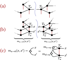
Figure 1: BP messages on a tree PEPS TN. (a) A local patch of a PEPS defined on a tree. The $(a,b)$ edge defines a bi-partition of the system into two branches. (b) The TN that corresponds to ${\langle{\psi}|{\psi}\rangle}$. Also here the $(a,b)$ edge defines two branches. The tensors that result from the contraction of each branch are the messages $m_{a\to b}(x,x^{\prime})$ and $m_{b\to a}(x,x^{\prime})$. (c) The messages satisfy a recursion relation, which are used to define the BP equations (2).

Consider a double layer TN that corresponds to the scalar ${\|\psi\|}^{2}={\langle{\psi}|{\psi}\rangle}$ (Fig. 1b). When $G=(V,E)$ is a tree (like an MPS, for example), it can be contracted efficiently using dynamical programming. One way to preform it is as follows. Given two incident nodes, $a,b$, the edge that connects them divides the system into two parts, see Fig. 1a,b. We define the “message” $m_{a\to b}(x,x^{\prime})$ to be the tensor that results from contracting the branch of ${\langle{\psi}|{\psi}\rangle}$ that is connected to $a$, where $(x,x^{\prime})$ are the indices of the open ket-bra edges connected to node $a$. Similarly, the message $m_{b\to a}(x,x^{\prime})$ is related to the contraction over the branch of $b$. See Fig. 1a,b. If we consider them as matrices of the indices $(x,x^{\prime})$, they are positive semi-definite, due to the fact that they are a result of a contraction of a branch with its complex conjugate. Crucially, these messages satisfy a recursive relation. If $N_{a}$ is the set of nodes that are incident to $a$, then the tensor $m_{a\to b}$ is given by the contraction

$$m_{a\to b}=\operatorname*{Tr}\Big{(}T_{a}T_{a}^{*}\prod_{a^{\prime}\in N_{a}\setminus\{b\}}m_{a^{\prime}\to a}\Big{)}$$ (1)

where $\operatorname*{Tr}(\cdot)$ denotes contraction of joint indices. For example, If $b,c,d$ are incident to $a$, then the message $m_{a\to b}(x,x^{\prime})$ is given in terms of the messages $m_{c\to a}(x,x^{\prime})$ and $m_{d\to a}(x,x^{\prime})$, as shown in Fig. 1c.

In principle, we can pick any node which is not a leaf, define it as a root, and use Eq. (1) to calculate the messages from the leaves to the root. Using the messages that lead to the root, we can calculate ${\|\psi\|}^{2}$. This calculation can also be done differently. Instead of forcing a particular causality order between the messages, we can try to solve Eq. (1) for all messages simultaneously. This can be done by solving Eq. (1) iteratively: starting from a set of random positive semi-definite (PSD) messages $\{m^{(0)}_{a\to b}(x,x^{\prime})\}$ for all incident nodes $a,b$, we define the set of messages at step $t+1$ using the messages of step $t$:

$$m^{(t+1)}_{a\to b}\stackrel{{\scriptstyle\mathrm{def}}}{{=}}\operatorname*{Tr}\Big{(}T_{a}T_{a}^{*}\prod_{a^{\prime}\in N_{a}\setminus\{b\}}m^{(t)}_{a^{\prime}\to a}\Big{)}.$$ (2)

Equation (2) is the BP equation for PEPS tensor-network. It is a natural extension of the BP equations for graphical models Wainwright and Jordan (2008); Koller and Friedman (2009); Mezard and Montanari (2009). The equation also guarantees that if the messages at $t$ are PSD when viewed as a matrix whose $(x,x^{\prime})$ element is $m_{a\to b}(x,x^{\prime})$, then so would the messages at $t+1$ be. The fixed point of this iterative process will solve Eq. (1), and give us all the $m_{a\to b}(x,x^{\prime})$ messages. It is a well-known fact that the BP iterations on tree graphical models have a unique fixed point to which they converge in linear number of steps ref . The same arguments easily generalizes also to our case. Once we have the messages, we can use the fact that they are contractions over branches, and use them to calculate local reduced density matrices (RDM). For example, the calculation of 2-local RDMs are shown in Fig. 2. The PSD property of the messages guarantees the resultant RDMs are also PSD.

Figure 2: In a tree, the converged BP messages can be used to calculated the local RDMs. In this example, a 2-local RDM. The same formulas are used to approximate the local RDMs also when the underlying PEPS is not a tree.

Thus far, the BP equations (2) might seem no more than an elegant method for contracting tree PEPS. Things become interesting when we consider graphs with loops. In such case, the messages can no longer be defined as contraction of branches, since an edge in the graph no longer partitions it into two distinct branches. Yet we can still define them as solutions to Eq. (1), and try to find them iteratively using Eq. (2). If the iterations converge to a fixed point, we can use the messages to estimate local marginals, using the same expressions as we did in the case of trees, which are illustrated in Fig. 2. This procedure is called loopy BP. Evidently, this is an uncontrolled approximation. In fact, there is no guarantee the BP iterations will converge to a fixed point, or that there is a unique fixed point. Nevertheless, in the world of graphical models, the BP method often provides surprisingly good results, in particular when the graph looks locally like a tree and there are no long-range correlations. A famous example are problems related to the decoding of error correction codes, in which BP performs extremely well McEliece et al. (1998). As we shall see, also in the world of tensor-networks loopy BP often performs well on problems with short-range entanglement.

While a general theory to explain the performance of the BP algorithm is still lacking, there are some partial results in this direction. An important result is due to Yedidia et al Yedidia et al. (2001), who established the correspondence between fixed points of the BP algorithm and the Bethe-Peierls approximation Bethe (1935). The Bethe-Peierls approximation is an approximation scheme for classical statistical mechanics, in which one treats the system as if its defined on a tree (a Bethe lattice). This assumption implies that the Gibbs distribution of the system, as well as the free-energy functional can be written as functions of the local marginals. When the actual interaction graph of the system is not a tree, this is an uncontrolled approximation. Nevertheless, also in these cases, one can take the Bethe free-energy functional and look for locally consistent set of marginals that minimizes it. This procedure often gives surprisingly good approximations. Yedidia et al Yedidia et al. (2001) showed that there is a 1-to-1 correspondence between extermum points of the Bethe free-energy and fixed points of the BP equations. The marginals obtained from the messages at a fixed point minimizes the Bethe free-energy, and conversely, from the marginals at the extremum point one can derive fixed-point messages of BP.

As we show in Appendix A, this result naturally generalizes to our case. The idea is that our BP algorithm for PEPS is the usual BP algorithm that is applied to a graphical model with complex entries, obtained from the tensor-network of ${\langle{\psi}|{\psi}\rangle}$. Such graphical models were studied in LABEL:ref:Cao2017-DEFG, under the name Double Edge Factor Graph (DEFG), where it was argued that the BP algorithm corresponds, like in the usual case, to the extreme points of the Bethe free-energy.

At this point it seems tempting to benchmark the BP algorithm for PEPS contraction, and compare it to other methods. Indeed, we first used the BP algorithm as a contraction subroutine in an imaginary time evolution algorithm on various 2D models, and compared to the performance of the simple update method Alkabetz (2020). Surprisingly, the final energies of both algorithms were suspiciously close to each other. As we show next, this can be explained theoretically; the mean field approximation at the heart of the simple-update method and the BP algorithm are equivalent.

III The simple update method

The simple-update method Jiang et al. (2008) is a direct generalization of the TEBD Vidal (2003, 2004); Daley et al. (2004) algorithm for 1D real and imaginary times evolution to higher dimensions. It calculates the dynamics of many-body spin systems that sit on a lattice, and are described by a (quasi-) canonical PEPS tensor-network. The method is efficient and numerically stable, but often results in poor accuracy due to its oversimplified representation of local environments.

At its core lies a quasi-canonical form of the PEPS that allows a crude approximation of local TN environments. This approximation is often referred to as mean field approximation. When the PEPS is in the shape of a tree, this form is truly canonical: it corresponds to consecutive Schmidt decompositions of the many-body quantum state. Every edge in the graph connects two disjoint branches of the system, which correspond to the Schmidt decomposition between these two branches ${|{\psi}\rangle}=\sum_{i=1}^{D}\lambda_{i}{|{L_{i}}\rangle}\otimes{|{R_{i}}\rangle}$. Specifically, the TN consists of two types of tensors: tensors $T_{a}$ that are connected to the physical legs, and diagonal $\lambda$ tensors that sit in the middle of every edge and correspond to the Schmidt weights, as illustrated in Fig. 3. The orthonormality of the Schmidt decomposition, and its correspondence with the TN structure implies that contraction over branches of the tree is given by a simple Kronecker delta function (Fig. 3b). Therefore, the RDMs of a given region can be readily computed using only the tensors that surround it (Fig. 3c), and in addition the tensors must satisfy local canonical conditions shown in (Fig. 3b). This type of approximation is often referred to as mean field approximation of the environment in the TN literature.

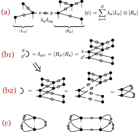
Figure 3: The properties of a canonical representation of a tree PEPS. (a) An example of a canonical representation of a tree PEPS and its relation to the Schmidt decomposition. The empty circles are diagonal tensors that correspond to the Schmidt weights $\lambda$. (b1) The orthonormality of the Schmidt bases implies a simple formula for the contraction of the left and right branches and (b2) a local canonical condition on the PEPS tensors. (c) A local expression for the reduced density matrices.

When the underlying graph has loops, the canonical form is no longer well-defined; removing an edge from the graph no longer divides it into two parts, and so it cannot be associated with a Schmidt decomposition between two branches. Nevertheless, we can still define a PEPS to be quasi-canonical if it satisfies the local canonical constraints of Fig. 3b2. In such case, the expression for local RDMs (e.g., Fig. 3c) is no longer exact. Nevertheless, when the graph looks locally like a tree, or when the quantum state has only short-range correlations, this approximation is often reasonable.

In the simple-update algorithm one usually starts from a quasi-canonical PEPS and then applies local gates that performs real or imaginary time evolution according the Trotter-Suzuki decomposition. For example, in the imaginary time evolution, if the Hamiltonian interaction term between the neighboring sites $a,b$ is $h_{ab}$, the operator $U_{ab}=e^{-\delta\tau h_{ab}}$ will be applied, where $\delta\tau$ is a small Trotter-Suzuki time step. Once $U_{ab}$ is applied, a local SVD decomposition is performed, as shown in Fig. 4b-f, which guarantees that: (i) the resultant tensor network can be reshaped into a local PEPS with $T_{a},\lambda,T_{b}$ replaced by $T_{a}^{\prime},\lambda^{\prime},T_{b}^{\prime}$ (ii) a truncation is performed so that the bond dimension of new tensors does not increase, and (iii) some of the local canonical conditions are (approximately) satisfied — see Fig. 4g.

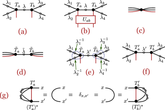
Figure 4: The Simple-Update steps of applying a “gate” $U_{ij}$ on the tensors $\{T_{i},\lambda,T_{j}\}$, and updating them to $\{T^{\prime}_{i},\lambda^{\prime},T^{\prime}_{j}\}$. (a) The original tensors. (b) Applying $U_{ij}$. (c) The $T_{a},T_{b}$ tensors and all surrounding $\lambda$ weights are contracted into one big tensor, which is reshaped as a matrix. (d) An SVD is performed on the matrix (e) and (f) a trivial $\lambda_{i}\lambda_{i}^{-1}$ pairs are inserted to the external legs and define the new $T_{a}^{\prime},\lambda^{\prime},T_{b}^{\prime}$ tensors. At this step, one can truncate the smallest weights of $\lambda^{\prime}$ to reduce the bond dimension back to $D$. (g) If no truncation was done, the resulting tensors satisfy some of the local canonical conditions.

When the operator $U_{ab}$ is not unitary (e.g., in the case ofs imaginary time evolution), or when truncation is performed, the resultant TN will no longer be quasi-canonical. Some of the canonical conditions will be satisfied, not all of them. However, also in that case, the $\lambda$ weights still provide a reasonable approximation for the local environments, as is evident by the success of the SU algorithm in many cases. In particular, in the imaginary time case, if the system reaches a fixed point, (the approximate ground state), it is also a fixed point of all the local SU steps. This state satisfies all the local canonical conditions, and is therefore a quasi-canonical state.

We conclude this section by noting that the SU steps can be easily turned into an algorithm for finding a quasi-canonical form of a PEPS TN. Starting from an arbitrary PEPS, we can apply a “trivial” SU step with $U_{ab}=\mathbbm{1}$, without the truncation step. In other words, we essentially perform an SVD decomposition of the fused tensor in Fig. 4d, which yields tensor $T_{a}^{\prime},\lambda^{\prime},T_{b}^{\prime}$ satisfying the local canonical condition of Fig. 4g. Repeating this step on all edges, if a fixed point is reached, it is by definition a quasi-canonical PEPS, and can be used to calculate local RDMs via the $\lambda$ weights (see Fig. 3c). We call this algorithm trivial-SU, and note that it has already been used previously (see, e.g., the quasi-orthogonalization in Sec. B of LABEL:ref:Kalis2012-SU, or the super-orthogonalization of LABEL:ref:Ran2012-Tucker). See also interesting parallels between our BP construction, the trivial-SU and the NCD theory of LABEL:ref:Ran2013-NCD (see also Chapter 5 in LABEL:ref:Ran2020-TN).

IV BP-SU equivalence

The trivial-SU algorithm and the BP algorithm for TN are two different algorithms for approximate contraction of PEPS. They originate from two very different places: the trivial-SU algorithm is a natural algorithm for TN, which relies on the Schmidt decomposition, whereas the BP algorithm is a message-passing algorithm for graphical models that originated from inference problems and the Bethe-Peierls approximation. It might therefore come as a surprise that these two algorithms are equivalent. In hindsight, this could have been anticipated, as both are iterative algorithms that are exact on trees. We prove

Theorem IV.1

Every trivial SU fixed point corresponds to a BP fixed point such that the local RDMs computed in both methods are identical.

As a simple corollary of this theorem we conclude that if the trivial SU equations and the BP equations have a unique fixed point, both algorithms will yield the same RDMs. In light of this equivalence, the success of the imaginary time SU algorithm for many models (see, for example, models analyzed in LABEL:ref:Jahromi2019-SU), is another example of the success of the Bethe-Peierls approximation.

To prove Theorem IV.1, we note that in the BP algorithm the TN remains fixed, while the BP messages evolve to a fixed point. In the trivial-SU, there are no messages, but the local tensors that make up the TN evolve until they converge to a quasi-canonical fixed-point, without changing the underlying quantum state. In both cases, the evolution is done via local steps. Our proof uses two lemma:

Lemma IV.2

Let $\mathcal{T},\mathcal{T}^{\prime}$ be two tensor-networks that represent the same state ${|{\psi}\rangle}$, such that $\mathcal{T}^{\prime}$ is obtained from $\mathcal{T}$ using a single trivial SU step on tensors $T_{a},T_{b}$ and the $\lambda$ weight between them. Then every BP fixed-point of $\mathcal{T}$ has a corresponding fixed-point of $\mathcal{T}^{\prime}$ with the same RDMs, and vice-versa.

The idea of the proof is to show that the fixed point messages of the new TN can be constructed from the fixed point messages of the old TN, except for the local place of change, where the messages are adapted to fit the new tensors. The full proof of the lemma is given in Appendix B.

Using this lemma repeatably along the trivial-SU iterations, we conclude that the BP fixed points of an initial TN is equivalent to those of its quasi-canonical representation. To finish the proof, we show that the BP fixed point of a quasi-canonical PEPS yields the same RDMs as the $\lambda$ weights do:

Lemma IV.3

Given a TN in a quasi-canonical form (i.e., a fixed point of the trivial SU algorithm), it has a BP fixed point that gives the same RDMs estimates as those of the quasi-canonical form based on the $\lambda$ weights.

The idea of the proof is that after “swallowing” a $\sqrt{\lambda}$ of each $\lambda$ tensor in its two adjacent $T_{a},T_{b}$ tensors, we reach a PEPS for which the messages $m_{a\to b}(x,x^{\prime})=\lambda_{x}\delta_{x,x^{\prime}}$ are a BP fixed-point. The full proof is found in Appendix B.

V Numerical tests.

In this section we present some numerical tests that compare the BP method to the trivial simple-update method. The asymptotic complexity of one step in both algorithms is similar. For example, on a square grid with virtual bond dimension $D$ and physical bond dimension $d$, both steps take $O(dD^{5})$ basic arithmetic operations. What might be more interesting is the number of iterations needed for convergence, which can be tested numerically. We compared these numbers on two types of PEPS on finite square grids. One type was a random PEPS with normal complex entries and the other was an approximate ground state of the anti-ferromagnetic Heisenberg model on a square lattice with random, nearest-neighbors coupling. For every model we ran the BP algorithm and the trivial-SU algorithm on $20-50$ random instances to calculate the 2-body RDMs. For each instance we calculated the ratio of the convergence time (i.e., number of iterations until convergence) $T_{BP}/T_{tSU}$. The results are given in Table 1. While for the random PEPS instances the BP method seems slightly faster, in the AFH models, where correlations are of longer range, the trivial-SU seems to converge faster, in particular as the bond dimension $D$ increases. The full histogram of the results, as well as the full numerical details can be found in Appendix C.

	Random-PEPS			AFH
	$4\times 4$	$10\times 10$		$4\times 4$	$10\times 10$
$D=2$:	$0.7\pm 0.2$	$0.6\pm 0.2$		$1.4\pm 0.1$	$1.3\pm 0.1$
$D=3$:	$0.7\pm 0.2$	$0.7\pm 0.2$		$1.1\pm 0.2$	$1.2\pm 0.1$
$D=4$:	$0.7\pm 0.2$	$0.8\pm 0.2$		$1.6\pm 0.5$	$1.8\pm 0.2$

Table 1: Average ratio of convergence times $T_{BP}/T_{tSU}$, together with standard deviations for random PEPS and ground states of anti-ferromagnetic Heisenberg model (AFH) with random n.n. couplings on a $N\times N$ lattices. We simulated different bond dimensions $D=2,3,4$ using $20-50$ realizations for each configuration. Full details can be found in Appendix C.

VI Discussion

In this work we established a bridge between the world of graphical models and tensor networks. We have defined the Belief Propagation method for PEPS contraction, which can be viewed as the ordinary BP method applied for Double Edge Factor Graphs (DEFG) Cao and Vontobel (2017) that are derived from the PEPS tensor network. Just as in the ordinary graphical models case, the fixed points of the BP iterations correspond to extreme points of the Bethe free-energy, which is defined for the underlying PEPS TN. We have shown that the BP algorithm is equivalent to the trivial SU algorithm on PEPS tensor networks, which leads to a quasi-canonical form. This correspondence has some interesting implications. First, since the fixed points of the imaginary time SU algorithm is a quasi-canonical PEPS, our result implies that its SU approximate environments correspond to a Bethe-Peierls approximation. The success of the SU algorithm can therefore be seen as another example of the power of the Bethe-Peierls approximation. Second, it shows that one of the simplest algorithms for approximating marginals in the world of graphical models is equivalent to one of the simplest approximate contraction algorithms in the world of tensor networks.

The equivalence of these two methods, which come from different fields and are derived from different principles, is interesting for several reasons. From the practical point of view, we can try to “import” other, more sophisticated algorithms for marginal approximations to the world of tensor networks. A natural candidate is the Generalized Belief-Propagation (GBP) algorithm Yedidia et al. (2001), which generalizes the BP algorithm by considering messages from larger regions in the graph. Just as the BP algorithm converges to extreme points of the Bethe free-energy, the GBP algorithm converges to extreme points of the Kikuchi free-energy of the cluster variation method Kikuchi (1951); Morita et al. (1994). As shown in LABEL:ref:Yedidia2001-GBP, this algorithm provides a much better approximation of the marginals, at the price of a higher computational cost. It would be interesting to compare the performance of this algorithm, as well as other BP improvements Montanari and Rizzo (2005); Chertkov and Chernyak (2006); Mooij et al. (2007); Nachmani et al. (2016); Cantwell and Newman (2019), when acting on TNs to that of more accurate contraction algorithms, such as the corner transfer method (CTMRG) Orús and Vidal (2009); Nishino and Okunishi (1996), the tensor-network renormalization group (TRG) Levin and Nave (2007); Gu et al. (2008) and boundary MPS (bMPS) Jordan et al. (2008), to name a few.

From the theoretical prospective, it would be interesting to better understand the physical and mathematical role of the complex Bethe free-energy that we have derived. In particular, we know that for tree-tensor networks, it is related to the Schmidt decomposition. Can we somehow relate it to the underlying entanglement structure also when the underlying graph has loops? Another interesting question is whether the BP equations can be used to analytically analyze models for which the ground state is a known PEPS, such as the AKLT model.

VII Acknowledgments

The authors thank Eyal Bairy, Raz Firanko, Roman Orús and Yosi Avron for their help with the manuscript and many useful suggestions. IA acknowledges the support of the Israel Science Foundation (ISF) under the Individual Research Grant No. 1778/17.

Appendix A Graphical models, Belief Propagation and the mapping of PEPS tensor networks and double-edge factor graphs

In this section we give a very brief background to the subject of graphical models and the Belief Propagation algorithm, and then sketch a mapping between the PEPS tensor networks to a particular type of graphical models called double-edge factor graphs. Together, this will show that our BP algorithm for PEPS is essentially the usual BP algorithm applied to the mapped double-edge factor graphs, and the converged messages correspond to a Bethe-Peierls approximation.

A.1 Graphical models and Belief Propagation

Graphical models are a powerful tool for modeling multivariate probability distributions. They provide a succinct description of the statistical dependence of a set of random variables using graphs, and are used in fields such as bioinformatics, communication theory, statistical physics, combinatorial optimization, signal and image processing, and statistical machine learning to name a few. In this section we give a brief background on this tool and the BP algorithm. For a thorough review, we refer the reader to Refs. Wainwright and Jordan (2008); Koller and Friedman (2009); Mezard and Montanari (2009).

Roughly speaking, there are three main families of graphical models: Bayesian networks, Markov Random Fields (MRF), and factor graph graphical models. As the latter family supersedes the first two, we will concentrate on it.

A factor graph graphical model is a succinct description of probability distribution $P(x_{1},\ldots,x_{n})$ of a set of random variables $X_{1},X_{2},\ldots X_{n}$. It is given as a product

$$P(x_{1},\ldots,x_{n})=\frac{1}{Z}\prod_{a\in\mathcal{F}}f_{a}(\bm{x}_{a}),$$

where $\mathcal{F}$ is a collection of “factors” $f_{a}(\bm{x}_{a})$. These are non-negative functions of small subsets of variables $\bm{x}_{a}=(x_{i_{1}},x_{i_{2}},\ldots,x_{i_{k}})$. $Z\stackrel{{\scriptstyle\mathrm{def}}}{{=}}\sum_{\bm{x}}\prod_{a\in\mathcal{F}}f_{a}(\bm{x}_{a})$ is an overall normalization constant. A very natural distribution of that form appears in classical statistical mechanics. Given a local Hamiltonian $H(\bm{x})=\sum_{a\in\mathcal{F}}h_{a}(\bm{x}_{a})$, its Gibbs distribution is

$$P(\bm{x})=\frac{1}{Z}e^{-\beta H(\bm{x})}=\frac{1}{Z}\prod_{a\in\mathcal{F}}e^{-\beta h_{a}(\bm{x}_{a})}.$$

In this case $f_{a}(\bm{x}_{a})=e^{-\beta h_{a}(\bm{x}_{a})}$ and $Z$ is the partition function.

There is convenient graphical way to capture the relation between the various factors, using a so-called factor graph $\mathcal{G}=(\mathcal{V},\mathcal{F},\mathcal{E})$. This is a bipartite graph with two types of vertices: $\mathcal{V}=\{x_{1},x_{2},\ldots,x_{n}\}$ is the set of variables, also called nodes. The other set of vertices are the factors $\mathcal{F}=\{f_{1},f_{2},\ldots\}$. $\mathcal{E}$ is the set of edges, where an edge connects the node $x_{i}$ to the factor $f_{a}$ iff $f_{a}$ depends on $x_{i}$. For example, the factor graph in Fig. 5 corresponds to probability distributions of the form $P(x_{1},x_{2},x_{3})=\frac{1}{Z}f_{1}(x_{1},x_{2},x_{3})\cdot f_{2}(x_{1},x_{2})$.

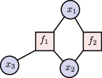
Figure 5: An example of a factor graph representing the probability distribution $P(x_{1},x_{2},x_{3})=\frac{1}{Z}f_{1}(x_{1},x_{2},x_{3})\cdot f_{2}(x_{1},x_{2})$.

Given a graphical model, a central task is to calculate its marginal over some small set of random variables. This is needed, for example, for the calculation of local expectation values, or for the optimization of the model with respect to empirical data. This task is NP-hard in general, involving a summation over an exponential number of configurations Cooper (1990).

Belief Propagation (BP) Pearl (1988); Wainwright and Jordan (2008); Koller and Friedman (2009); Mezard and Montanari (2009) is a message-passing algorithm that is designed to approximate such marginals. It is exact on graphical models whose underlying graph is a tree and often gives surprisingly good results on loopy graphs. In these cases, however, it is essentially an uncontrolled heuristic. The BP algorithm is often known in different names at different contexts. In statistical physics, it is known as the ‘Bethe–Peierls approximation’ Bethe (1935); Peierls (1936), and in coding theory as ‘sum-product algorithm’ Kschischang et al. (2001). The name ‘belief propagation’ was coined by J. Pearl, who used it in the context of Bayesian networks Pearl (1988, 1982).

The main objects in the BP algorithm are “messages” between factor and nodes and vice versa. To write them, let us define $N_{i}$ as the set of factors in which $x_{i}$ participates, and similarly $N_{a}$ to be the set of variables of the factor $f_{a}$ (i.e., adjacent nodes to $f_{a}$). A message from a factor $f_{a}$ to an adjacent node $i\in N_{a}$ is a non-negative function $m_{a\to i}(x_{i})$ and a message from node $i$ to factor $a$ is a non-negative function $m_{i\to a}(x_{i})$. The BP algorithm starts by initializing the messages (say, randomly), and then at each step, the messages are updated from the messages of the previous step by the local rules (see also Fig. 6):

$$m^{(t+1)}_{i\to a}(x_{i}) \stackrel{{\scriptstyle\mathrm{def}}}{{=}}\prod_{b\in N_{i}\setminus\{a\}}m^{(t)}_{b\to i}(x_{i}),$$ (3)

$$m^{(t+1)}_{a\to i}(x_{i}) \stackrel{{\scriptstyle\mathrm{def}}}{{=}}\sum_{\bm{x}_{a}\setminus\{x_{i}\}}f_{a}(\bm{x}_{a})\prod_{j\in a\setminus\{i\}}m^{(t)}_{j\to a}(x_{j}).$$ (4)

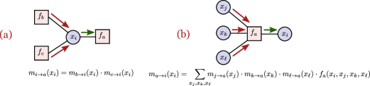
Figure 6: Illustration of the BP equations on a factor-graph graphical model — Eqs. (3,4). In such case there are two types of messages: nodes to factors (Fig. a, Eq. (3)) and factors to nodes (Fig. b, Eq. (4)).

If the messages converge to a fixed point, they can be used to estimate the marginals on subsets of nodes. For example, the marginal of a single variable $x_{i}$ is given by

$$P_{i}(x_{i})=\frac{1}{\mathcal{N}}\prod_{a\in N_{i}}m_{a\to i}(x_{i}),$$ (5)

where $\mathcal{N}$ is a normalization factor. The marginal over the variables of a factor are given by

$$P_{a}(\bm{x}_{a})=\frac{1}{\mathcal{N}}f_{a}(\bm{x}_{a})\prod_{i\in N_{a}}m_{i\to a}(x_{i}),$$ (6)

These two expressions are demonstrated in Fig. 7

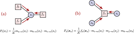
Figure 7: Calculating the local marginals from the BP messages by the formulas in Eqs. (5,6). These formulas give the exact marginals when the underlying graphical model is a tree.

For tree graphical models, the BP messages are promised to converge to a unique fixed point in linear time, and formulas (5, 6) give the exact marginals ref .

When the underlying graph has loops, the BP algorithm is called ‘loopy BP’, and the formulas for the marginals become, essentially, uncontrolled. Moreover, it is not known how fast the algorithm will converge, if ever, or if it has a unique fixed point. Nevertheless, in many practical cases, the loopy BP provides surprisingly good result.

While, a general theory to explain the performance of BP algorithm is still lacking, there are some partial results in this direction. An important result is due to Yedidia et al Yedidia et al. (2001), who highlighted the correspondence between the Bethe-Peierls approximation and fixed points of the BP algorithm, which we now explain briefly. The starting point are models defined on tree graphs. A simple observation is that for these models, the global probability distribution can be written in terms of its local marginals:

$$P(\bm{x})=\prod_{a\in\mathcal{F}}P_{a}(\bm{x}_{a})\prod_{i\in\mathcal{V}}\big{(}P_{i}(x_{i})\big{)}^{1-d_{i}},$$ (7)

where $P_{a}(\bm{x}_{a})$ is the marginal on the nodes adjacent to $a\in\mathcal{F}$, and $P_{i}(x_{i})$ is the marginal of $x_{i}$. Finally, $d_{i}=|N_{i}|$ is the number of factors that are adjacent to $x_{i}$. Using Eq. (7), we can write the free energy in terms of the local marginals:

$$F_{Bethe}=\sum_{a}\sum_{\bm{x}_{a}}P_{a}(\bm{x}_{a})\ln\frac{P_{a}(\bm{x}_{a})}{f_{a}(\bm{x}_{a})}-\sum_{i}(d_{i}-1)\sum_{x_{i}}P_{i}(x_{i})\ln P_{i}(x_{i}).$$ (8)

The above expression is called the Bethe free-energy. When the underlying graph is not a tree, the Bethe free-energy is still well defined, but no longer equal the exact free-energy. In such case, we can use it to approximate the local marginals. We write the Bethe free-energy as a function of unknown marginals $\{q_{a}(\bm{x}_{a}),q_{i}(x_{i})\}$, and then we estimate the real marginals $\{P_{a}(\bm{x}_{a}),P_{i}(x_{i})\}$ by finding the $\{q_{a}(\bm{x}_{a}),q_{i}(x_{i})\}$ that minimize the Bethe free-energy. This procedure is exact on trees, where the Bethe free-energy is equal to the exact free energy, but on loopy graphs it is essentially an uncontrolled approximation; the resultant $q_{a}(\bm{x}_{a}),q_{i}(x_{i})$, may be far from the actual marginals, and in fact, they might not be marginals of any underlying global distribution. Nevertheless, decades of experience in statistical mechanics has shown that this is often a good approximation that gives better results than simple mean field. In LABEL:ref:Yedidia2001-GBP it was showen that there is a one-to-one connection between the fixed-points of the BP equations and the extreme points of the Bethe free-energy. The Lagrange multipliers used to minimize the latter become the fixed-point BP messages, and the local marginals coincide. This connection between a message-passing inference algorithm, and a variational approach gave rise to a plethora of other message-passing algorithms, such as generalized belief propagation (GBP), which are based on more sophisticated free energies, such as Kikuchi’s cluster variation method Kikuchi (1951)

A.2 Mapping a PEPS tensor network to a graphical model

In this section we present a mapping that takes a PEPS TN to a graphical model. Relations and dualities between graphical models and tensor networks have been studied over the years by several authors Critch and Morton (2014); Robeva and Seigal (2018); Chen et al. (2018). Our approach shares some similarities with these works, but in particular builds on the Double Edge Factor Graph (DEFG) formalism of LABEL:ref:Cao2017-DEFG. This allows us to transform a tree tensor-network into a tree graphical model, and it also has the desirable property of messages being positive semi-definite matrices.

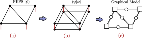
Figure 8: Mapping a tensor network to a graphical model of type double edge factor graph.

Figure 9: Defining the complex $f_{a}(\bm{z}_{a})$ factors from the PEPS tensors $T_{a}$, via $f_{a}(\bm{z}_{a})\stackrel{{\scriptstyle\mathrm{def}}}{{=}}\operatorname*{Tr}(T_{a}T_{a}^{*})$. $z_{i}\stackrel{{\scriptstyle\mathrm{def}}}{{=}}(x_{i},x_{i}^{\prime})$ that originate from the ket and the bra of the ${\langle{\psi}|{\psi}\rangle}$ TN.

The mapping between PEPS and DEFG is illustrated in Fig. 8. Let ${|{\psi}\rangle}$ be the many-body quantum state that is described by our TN, and consider the tensor network corresponding to ${\langle{\psi}|{\psi}\rangle}$, in which, we clump every edge in ${|{\psi}\rangle}$ with its equivalent edge in ${\langle{\psi}|}$ (see Fig. 8b). We call such pairs of edges ‘double edges’. They run over $D^{2}$ values of the double indices $(x,x^{\prime})$ of the ket and the bra TN. We map this TN into a graphical model as follows:

• We associate every double edge with a node so that its double indices $(x_{i},x_{i}^{\prime})$ now become a single variable in the graphical model. We denote this pair by a single variable $z_{i}=(x_{i},x_{i}^{\prime})$, and notice that it runs over $D^{2}$ discrete values.

• We associate the contraction of every pair $T_{a},T^{*}_{a}$ of bra-ket local tensors along their physical leg with a factor. See Fig. 8b,c. Specifically, let $T^{\mu}_{a;x_{1},\ldots,x_{k}}$ be the PEPS tensor at node $a$ with $\mu$ being the physical leg, then the resultant factor is given by

  $$f_{a}[z_{1},\ldots,z_{k}]\stackrel{{\scriptstyle\mathrm{def}}}{{=}}f_{a}\big{[}(x_{1},x^{\prime}_{1}),\ldots,(x_{k},x_{k}^{\prime})\big{]}\stackrel{{\scriptstyle\mathrm{def}}}{{=}}\sum_{\mu=1}^{d}T^{\mu}_{a;x_{1},\ldots,x_{k}}\cdot\Big{(}T^{\mu}_{a;x^{\prime}_{1},\ldots,x^{\prime}_{k}}\Big{)}^{*}$$ (9)

  See Fig. 9. As in the body of the paper, we write $\bm{x}_{a}=(x_{1},\ldots,x_{k})$, $\bm{x}^{\prime}_{a}=(x^{\prime}_{1},\ldots,x^{\prime}_{k})$, and $\bm{z}_{a}=(z_{1},\ldots,z_{k})$ for the variables of the factor $a$. With this notation, we may write $f_{a}(\bm{z}_{a})=f_{a}(\bm{x}_{a},\bm{x}_{a}^{\prime})$. Definition 9 immediately implies that as a matrix, $f_{a}(\bm{x}_{a},\bm{x}_{a}^{\prime})$ is positive semi-definite.

• Graphically, variable nodes are denoted by circles, and factors by squares. Adjacent variables and factors are connected by double lines (edges) that correspond to the double variable $z_{i}=(x_{i},x_{i}^{\prime})$ that they represent. See Fig. 8.

With these definitions, the resultant graphical model is called a DEFG and describes the function

$$P(\bm{z}) \stackrel{{\scriptstyle\mathrm{def}}}{{=}}P(z_{1},\ldots,z_{n})=\frac{1}{Z}\prod_{a}f_{a}(\bm{z}_{a}), Z \stackrel{{\scriptstyle\mathrm{def}}}{{=}}\sum_{\bm{z}}\prod_{a}f_{a}(\bm{z}_{a})={\langle{\psi}|{\psi}\rangle}.$$ (10)

Writing $P(\bm{z})$ as $P(\bm{x},\bm{x}^{\prime})$, the positivity of the individual $f_{a}(\bm{x}_{a},\bm{x}^{\prime}_{a})$ implies that also $P(\bm{x},\bm{x}^{\prime})$ is a positive semi-definite function. We can therefore interpret it as the density matrix of some fictitious quantum states that “lives on the edges of the PEPS”, although it has a non-conventional normalization because $\operatorname*{Tr}P=\sum_{\bm{x},\bm{x}}P(\bm{x},\bm{x})$ is not necessarily equal to $1$ (instead, it is $\sum_{\bm{x},\bm{x}^{\prime}}P(\bm{x},\bm{x}^{\prime})=1$).

Once the factor graphical model is defined, we can run the BP iterations on it,

$$m^{(t+1)}_{i\to a}(z_{i}) \stackrel{{\scriptstyle\mathrm{def}}}{{=}}\prod_{b\in N_{i}\setminus\{a\}}m^{(t)}_{b\to i}(z_{i}),$$ (11)

$$m^{(t+1)}_{a\to i}(z_{i}) \stackrel{{\scriptstyle\mathrm{def}}}{{=}}\sum_{\bm{z}_{a}\setminus\{z_{i}\}}f_{a}(\bm{z}_{a})\prod_{j\in a\setminus\{i\}}m^{(t)}_{j\to a}(z_{j}).$$ (12)

which are simply the usual BP equations (3, 4) with $x_{i}$ replaced by the double-edge variable $z_{i}$. It is easy to see that these equations are equivalent to Eq. (2) in the paper by noting that every node $i$ is adjacent to exactly two factors $a,b$ (because it corresponds to an edge in the PEPS connecting two vertices), and therefore by Eq. (11),

$$m^{(t+1)}_{i\to b}(z_{i})=m^{(t)}_{a\to i}(z_{i}),$$

which we identify with $m^{(t+1)}_{a\to b}$ from Eq. (2). Moreover, the summation $\sum_{\bm{z}_{a}\setminus\{z_{i}\}}$ in Eq. (12) is exactly the contraction of the virtual legs in Eq. (2) and Fig. 1c. Finally, note that as $f_{a}(\bm{x}_{a},\bm{x}^{\prime}_{a})$ are positive semi-definite, then Eqs. (11, 12) imply that if the messages at time $t$ are positive semi-definite then so are the messages at $t+1$.

The above discussion shows that like in the ordinary graphical models, also here fixed points of the BP iterations are solving a Bethe-Peierls type of approximation. In particular, defining the local “marginals”

$$P_{a}(\bm{z}_{a}) \stackrel{{\scriptstyle\mathrm{def}}}{{=}}\sum_{\bm{z}\setminus\bm{z}_{a}}P(\bm{z}), P_{i}(\bm{z}_{i}) \stackrel{{\scriptstyle\mathrm{def}}}{{=}}\sum_{\bm{z}\setminus\{z_{i}\}}P(\bm{z}).$$

We can write a complex Bethe free-energy

$$F_{Bethe}=\sum_{a}\sum_{\bm{z}_{a}}P_{a}(\bm{z}_{a})\ln\frac{P_{a}(\bm{z}_{a})}{f_{a}(\bm{z}_{a})}-\sum_{i}(d_{i}-1)\sum_{z_{i}}P_{i}(z_{i})\ln P_{i}(z_{i}),\qquad z_{i}=(x_{i},x_{i}^{\prime}),$$ (13)

which is defined by first choosing a specific branch of the logarithmic function. Note that in this case, $d_{i}=|N_{i}|=2$ because there are always exactly two adjacent factors to each variable $z_{i}$, and so

$$F_{Bethe}=\sum_{a}\sum_{\bm{z}_{a}}P_{a}(\bm{z}_{a})\ln\frac{P_{a}(\bm{z}_{a})}{f_{a}(\bm{z}_{a})}-\sum_{i}\sum_{z_{i}}P_{i}(z_{i})\ln P_{i}(z_{i}).$$ (14)

It is not very hard to show that the even though $P_{a}(\bm{z}),P_{i}(z_{i}),f_{a}(\bm{z}_{a})$ might take complex values, $F_{Bethe}$ must be real. In LABEL:ref:Cao2017-DEFG it was argued that also in this case fixed points of the BP iterations correspond to extremum points of the above functional. We note, however, that unlike the ordinary case, we see no reason why the complex Bethe free-energy should be positive. Interestingly, in all of our numerics, it was positive.

Appendix B Proofs of Lemmas IV.2,IV.3

B.1 Proof of Lemma IV.2

Assume a trivial-SU step changes the TN $\mathcal{T}$ to $\mathcal{T}^{\prime}$ by locally changing the adjacent tensors $T_{a},\lambda,T_{b}$ to $T^{\prime}_{a},\lambda^{\prime},T^{\prime}_{b}$, while keeping the rest of the tensors fixed (see Fig. 4a-f with trivial $U_{ab}=\mathbbm{1}$). To simplify the book-keeping, we “swallow” the $\lambda$ tensors in the $T_{a}$ tensors by splitting every $\lambda$ tensor into $\lambda=\sqrt{\lambda}\cdot\sqrt{\lambda}$ and contracting each $\sqrt{\lambda}$ with its adjacent $T_{a}$ tensor, see Fig. 10. We denote the resulting tensor networks by $\mathcal{F},\mathcal{F}^{\prime}$, and note that their local tensors are identical except for the $F_{a},F_{b}$ and $F_{a}^{\prime},F^{\prime}_{b}$ which are equal to the $T_{a},T_{b},T_{a}^{\prime},T_{b}^{\prime}$ tensors contracted with the appropriate $\sqrt{\lambda}$ tensors. The fact that the contraction of $(T_{a},\lambda,T_{b})$ is equal to the contraction of $(T_{a}^{\prime},\lambda^{\prime},T_{b}^{\prime})$ implies that the contraction of $(F_{a},F_{b})$ is equal to the contraction of $(F_{a}^{\prime},F_{b}^{\prime})$.

Figure 10: Swallowing the $\lambda$ weights in the $T$ tensors and obtaining an equivalent TN with $F$ tensors. The empty circles denote a Simple-Update weight tensor $\lambda_{x}\delta_{xy}$ and the red circle denote its square root: $\sqrt{\lambda_{x}}\delta_{xy}$.

Let $\{m_{a\to b}(x,x^{\prime})\}$ be fixed-point BP messages of $\mathcal{F}$. We will use these messages to construct fixed-point BP messages $\{m^{\prime}_{a\to b}(x,x^{\prime})\}$ of $\mathcal{F}^{\prime}$ that give the same RDMs. All messages except for the $a\to b$ and $b\to a$ messages remain the same. The $a\to b$ and $b\to a$ messages are defined by the BP iterative equations using the new tensors $F^{\prime}_{a},F^{\prime}_{b}$ so that they will satisfy them. For example, if tensor $F_{a}$ is connected also to tensors $F_{c},F_{d}$ in addition to $F_{b}$, then $m^{\prime}_{a\to b}(x,x^{\prime})$ is given by the diagram in Fig. 1c, replacing $T$ tensors by corresponding $F^{\prime}$ tensors. To finish the proof, we need to show that this new set of messages (i) is a BP fixed-point, and (ii) produces the same RDMs according to the BP formula (see Fig. 2). Clearly, for adjacent vertices that have nothing to do with $a,b$, both conditions hold trivially, as the relevant messages and underlying tensors are unchanged. Let us then verify these points for vertices in the vicinity of $a,b$.

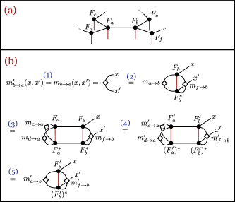
Figure 11: (a) The description of the TN. canonical condition. (b) Proving that $m^{\prime}_{b\to e}$ is given by the BP propagation of messages $m^{\prime}_{a\to b}$ and $m^{\prime}_{f\to b}$: Equality (1) follows from definition, $m^{\prime}_{b\to e}=m_{b\to e}$. Then in (2) we use the assumption that $m_{b\to e}$ is a fixed point of the BP equation, and similarly in (3) we use that assumption on $m_{a\to b}$. In (4) we use the fact that the contraction of $F_{a},F_{b}$ is equal to the contraction of $F_{a}^{\prime},F_{b}^{\prime}$, together with the definitions that all the new messages are equal to the old messages, except for the $a\leftrightarrow b$ messages. Finally, in (5) we use the definition of $m^{\prime}_{a\to b}$ which was designed to satisfy the BP equations.

Checking point (i):

By definition, the $a\to b$ and $b\to a$ messages satisfy the BP equations. So we only need to verify that other messages from $a$ or $b$ (but not between them) satisfy the BP equations. Consider, for example, the message $b\to e$ in Fig. 11a. We need to verify that $m^{\prime}_{b\to e}(x,x^{\prime})$ is indeed a BP fixed-point, given as the appropriate expression of $m^{\prime}_{a\to b},m^{\prime}_{f\to b}$ (see Fig. 1c for the BP equations). This is proved in Fig. 11b in a series of 5 simple equalities (see the caption for full explanation), which rely on the fact that the original messages are fixed point of the BP equations, and that the contraction of $F_{a},F_{b}$ is equal to the contraction of $F^{\prime}_{a},F^{\prime}_{b}$.

Checking point (ii):

By definition if we are interested in 2-body RDMs on vertices that are different from both $a$ and $b$, then the RDM estimate will remain the same because neither the relevant messages, nor the tensors changed. We only need to verify for the RDM $\rho_{ab}$ and RDMs that contain $a$ or $b$ with other adjacent node, such as $\rho_{be}$. For the former, $\rho_{ab}=\rho^{\prime}_{ab}$ because it depends on the incoming messages to the $a,b$ nodes (which remain the same), together with the contraction of $F^{\prime}_{a},F^{\prime}_{b}$, which by assumption is identical to that of $F_{a},F_{b}$. For the latter, the proof uses the same idea as in point (i). Using the assumption that the contraction of $F_{a},F_{b}$ is identical to that of $F_{a}^{\prime}F_{b}^{\prime}$, and that $F_{e}^{\prime}=F_{e}$, it is easy to show that the 3-body RDM $\rho_{abe}$ is identical to that of $\rho_{abe}^{\prime}$, from which we deduce that $\rho_{be}=\rho^{\prime}_{be}$. This concludes the proof of Lemma IV.2.

B.2 Proof of Lemma IV.3

As in the first lemma, we first define $\mathcal{F}$ to be an equivalent TN in which every $\lambda$ weight tensor in $\mathcal{T}$ was split into $\sqrt{\lambda}\cdot\sqrt{\lambda}$ and the $\sqrt{\lambda}$ tensors are contracted into the $T_{a}$ tensors to give the $F_{a}$ tensors (see Fig. 10). Next we define a set of messages

$$m_{a\to b}(x,x^{\prime})\stackrel{{\scriptstyle\mathrm{def}}}{{=}}\lambda_{x}\delta_{x,x^{\prime}}$$ (15)

for every two adjacent vertices $a,b$, where $\lambda$ is the weight on the $ab$ edge in the original $\mathcal{T}$ tensor. We claim that (i) these messages are BP fixed-point on the $\mathcal{F}$ TN, and (ii) they give the same 2-body RDMs as those of the trivial SU method of quasi-canonical $\mathcal{T}$. Both claims are immediate. Claim (i) follows by writing the BP equation for the $a\to b$ message in terms of the $F_{a}$ tensor, and noticing that this expression is equal to it gives the $\lambda_{x}\delta_{x,x^{\prime}}$ using canonical condition on $\mathcal{T}$. This is illustrated in Fig. 12. Claim (ii) follows from definitions of the 2-body RDMs of the BP method and the SU method (see Fig. 3e, and Fig. 2).

Figure 12: The proof of Lemma IV.3: defining the BP messages by Eq. (15) and using the canonical condition shows that these messages are fixed point of the BP equations.

Appendix C Numerical results

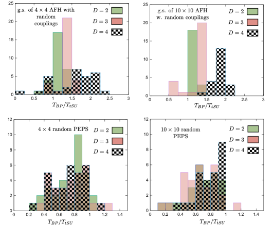
Figure 13: The ratio of the number of iterations that takes the BP algorithm to converge by that of the trivial-SU algorithm. The tests were on $4$ different systems: a $4\times 4$ and $10\times 10$ anti-ferromagnetic Heisenberg models with random coupling, as well as $4\times 4$ and $10\times 10$ random PEPS. For one of these 4 cases, PEPS were used with bond dimension $D=2,3,4$, and the statistics was generated using $20-50$ different realizations. More details on the numerical procedure can be found the text body.

As part of this work, we ran simulations to compare the convergence times of BP to the ones of trivial-SU on different PEPS states. We tested the algorithms over two types of systems: $i)$ random PEPS, $ii)$ PEPS ground-states of the anti-ferromagnetic Heisenberg model (AFH) with random couplings

$$H =\sum_{{\langle{a,b}\rangle}}J_{ab}\bm{\sigma}_{a}\otimes\bm{\sigma}_{b}, J_{ab}<0.$$ (16)

Both systems were simulated on a $4\times 4$ and $10\times 10$ squared lattices. In all tests, the physical bond dimension was $d=2$ and virtual bond dimensions were $D=2,3,4$. All in all we therefore tested $2\times 2\times 3=12$ different configurations. For every configuration we used statistics of $20-50$ different random realizations on which we did the analysis.

In the random PEPS configurations, the tensor entries where chosen as $a+ib$, where $a,b$ were uniformly distributed in $(-1,1)$. In the AFH configurations, we used random couplings $J_{ab}$ uniformly distributed in the interval $(-1,0)$. To obtain the ground states of these models, we ran an imaginary time evolution with simple-update, with decreasing values of imaginary time steps by $\delta\tau=0.1,\dots,0.0001$. After obtaining an approximation to the ground state, we applied a random local gauge change on every bond in order to get a TN that is far away from a canonical form. Specifically, for every virtual edge $(a,b)$, we drew a random matrix $V_{ab}$ which was a product of a random unitary with a diagonal with random entries between $(0.5,2)$. We then inserted the identity $V_{ab}^{-1}V_{ab}=\mathbbm{1}$ in the middle of the edge, absorbing $V^{-1}_{ab}$ in $T_{a}$ and $V_{ab}$ in $T_{b}$. This way, the resultant TN was far from quasi-canonical, yet represented the same approximate ground state.

The convergence criteria for both BP and trivial-SU was taken with respect to the averaged trace distance of $2$-body RDMs between consecutive iterations (see Fig. 3c for trivial-SU and Fig. 2 for BP RDMs illustrations) such that $\frac{1}{m}\sum_{{\langle{a,b}\rangle}}{\|\rho_{ab}^{(t+1)}-\rho_{ab}^{(t)}\|}_{1}<10^{-6}$, where ${\langle{a,b}\rangle}$ denotes nearest-neighbors nodes and $m$ is the total number of such neighbors.

References

- Orús (2014) R. Orús, Annals of Physics 349, 117 (2014).
- Wainwright and Jordan (2008) M. J. Wainwright and M. I. Jordan, Foundations and Trends® in Machine Learning 1, 1 (2008).
- Koller and Friedman (2009) D. Koller and N. Friedman, Probabilistic graphical models: principles and techniques (MIT press, 2009).
- Mezard and Montanari (2009) M. Mezard and A. Montanari, Information, physics, and computation (Oxford University Press, 2009).
- Cooper (1990) G. F. Cooper, Artificial intelligence 42, 393 (1990).
- Schuch et al. (2007) N. Schuch, M. M. Wolf, F. Verstraete, and J. I. Cirac, Phys. Rev. Lett. 98, 140506 (2007).
- Markov and Shi (2008) I. L. Markov and Y. Shi, SIAM Journal on Computing 38, 963 (2008), https://doi.org/10.1137/050644756 .
- Orús and Vidal (2009) R. Orús and G. Vidal, Phys. Rev. B 80, 094403 (2009).
- Nishino and Okunishi (1996) T. Nishino and K. Okunishi, Journal of the Physical Society of Japan 65, 891 (1996), https://doi.org/10.1143/JPSJ.65.891 .
- Baxter (1968) R. J. Baxter, Journal of Mathematical Physics 9, 650 (1968).
- Baxter (1978) R. J. Baxter, Journal of Statistical Physics 19, 461 (1978).
- Sandvik and Vidal (2007) A. W. Sandvik and G. Vidal, Phys. Rev. Lett. 99, 220602 (2007).
- Wang et al. (2011) L. Wang, I. Pižorn, and F. Verstraete, Phys. Rev. B 83, 134421 (2011).
- Ferris and Vidal (2012) A. J. Ferris and G. Vidal, Phys. Rev. B 85, 165146 (2012).
- Levin and Nave (2007) M. Levin and C. P. Nave, Phys. Rev. Lett. 99, 120601 (2007).
- Efrati et al. (2014) E. Efrati, Z. Wang, A. Kolan, and L. P. Kadanoff, Rev. Mod. Phys. 86, 647 (2014).
- Robeva and Seigal (2018) E. Robeva and A. Seigal, Information and Inference: A Journal of the IMA 8, 273 (2018), https://academic.oup.com/imaiai/article-pdf/8/2/273/28864933/iay009.pdf .
- Pearl (1982) J. Pearl, in in Proceedings of the National Conference on Artificial Intelligence (1982) pp. 133–136.
- Kschischang et al. (2001) F. R. Kschischang, B. J. Frey, and H. . Loeliger, IEEE Transactions on Information Theory 47, 498 (2001).
- Bethe (1935) H. A. Bethe, Proceedings of the Royal Society of London. Series A-Mathematical and Physical Sciences 150, 552 (1935).
- Peierls (1936) R. Peierls (Cambridge University Press, 1936) p. 477–481.
- (22) See, for example, Theorem 14.1 in Ref. Mezard and Montanari (2009).
- McEliece et al. (1998) R. J. McEliece, D. J. C. MacKay, and Jung-Fu Cheng, IEEE Journal on Selected Areas in Communications 16, 140 (1998).
- Yedidia et al. (2001) J. S. Yedidia, W. T. Freeman, and Y. Weiss, in Advances in neural information processing systems (2001) pp. 689–695.
- Cao and Vontobel (2017) M. X. Cao and P. O. Vontobel, in 2017 IEEE Information Theory Workshop (ITW) (IEEE, 2017) pp. 136–140.
- Alkabetz (2020) R. Alkabetz, Using the Belief Propagation algorithm for finding Tensor Networks approximations of many-body ground states, Master’s thesis, Technion, Haifa, Israel (2020).
- Jiang et al. (2008) H. C. Jiang, Z. Y. Weng, and T. Xiang, Phys. Rev. Lett. 101, 090603 (2008).
- Vidal (2003) G. Vidal, Phys. Rev. Lett. 91, 147902 (2003).
- Vidal (2004) G. Vidal, Phys. Rev. Lett. 93, 040502 (2004).
- Daley et al. (2004) A. J. Daley, C. Kollath, U. Schollwöck, and G. Vidal, Journal of Statistical Mechanics: Theory and Experiment 2004, P04005 (2004).
- Kalis et al. (2012) H. Kalis, D. Klagges, R. Orús, and K. P. Schmidt, Phys. Rev. A 86, 022317 (2012).
- Ran et al. (2012) S.-J. Ran, W. Li, B. Xi, Z. Zhang, and G. Su, Phys. Rev. B 86, 134429 (2012).
- Ran et al. (2013) S.-J. Ran, B. Xi, T. Liu, and G. Su, Phys. Rev. B 88, 064407 (2013).
- Ran et al. (2020) S.-J. Ran, E. Tirrito, C. Peng, X. Chen, L. Tagliacozzo, G. Su, and M. Lewenstein, Tensor Network Contractions: Methods and Applications to Quantum Many-Body Systems (Springer Nature, 2020).
- Jahromi and Orús (2019) S. S. Jahromi and R. Orús, Phys. Rev. B 99, 195105 (2019).
- Kikuchi (1951) R. Kikuchi, Physical review 81, 988 (1951).
- Morita et al. (1994) T. Morita, M. Suzuki, K. Wada, and M. Kaburagi, Prog. Theor. Phys. Suppl. 115, 136 (1994).
- Montanari and Rizzo (2005) A. Montanari and T. Rizzo, Journal of Statistical Mechanics: Theory and Experiment 2005, P10011 (2005).
- Chertkov and Chernyak (2006) M. Chertkov and V. Y. Chernyak, Journal of Statistical Mechanics: Theory and Experiment 2006, P06009 (2006).
- Mooij et al. (2007) J. Mooij, B. Wemmenhove, B. Kappen, and T. Rizzo, in Artificial Intelligence and Statistics (2007) pp. 331–338.
- Nachmani et al. (2016) E. Nachmani, Y. Be’ery, and D. Burshtein, in 2016 54th Annual Allerton Conference on Communication, Control, and Computing (Allerton) (2016) pp. 341–346.
- Cantwell and Newman (2019) G. T. Cantwell and M. E. J. Newman, Proceedings of the National Academy of Sciences 116, 23398 (2019), https://www.pnas.org/content/116/47/23398.full.pdf .
- Gu et al. (2008) Z.-C. Gu, M. Levin, and X.-G. Wen, Phys. Rev. B 78, 205116 (2008).
- Jordan et al. (2008) J. Jordan, R. Orús, G. Vidal, F. Verstraete, and J. I. Cirac, Phys. Rev. Lett. 101, 250602 (2008).
- Pearl (1988) J. Pearl, Probabilistic Reasoning in Intelligent Systems: Networks of Plausible Inference (Morgan Kaufmann, 1988).
- Critch and Morton (2014) A. Critch and J. Morton, Symmetry, Integrability and Geometry: Methods and Applications (2014), 10.3842/SIGMA.2014.095.
- Chen et al. (2018) J. Chen, S. Cheng, H. Xie, L. Wang, and T. Xiang, Phys. Rev. B 97, 085104 (2018).