Estimating the logarithm of characteristic function and stability parameter for symmetric stable laws

Abstract

Let $X_{1},\ldots,X_{n}$ be an i.i.d. sample from symmetric stable distribution with stability parameter $\alpha$ and scale parameter $\gamma$. Let $\varphi_{n}$ be the empirical characteristic function. We prove an uniform large deviation inequality: given preciseness $\epsilon>0$ and probability $p\in(0,1)$, there exists universal (depending on $\epsilon$ and $p$ but not depending on $\alpha$ and $\gamma$) constant $\bar{r}>0$ so that

$$P\big{(}\sup_{u>0:r(u)\leq\bar{r}}|r(u)-\hat{r}(u)|\geq\epsilon\big{)}\leq p,$$

where $r(u)=(u\gamma)^{\alpha}$ and $\hat{r}(u)=-\ln|\varphi_{n}(u)|$. As an applications of the result, we show how it can be used in estimation unknown stability parameter $\alpha$.

Keywords: Stable laws, large deviation inequalities, parameter estimation;

MSC codes: Stable laws 60E07; Confidence regions 62F25

1 Introduction and preliminaries

Let $X_{1},\ldots,X_{n}$ be an i.i.d. sample from stable law with characteristic function $\varphi(u)=\exp\left[-(\gamma|u|)^{\alpha}+i\omega(u)\right]$, where $\omega(u)=u[\beta\gamma\tan\frac{\pi\alpha}{2}(|\gamma u|^{\alpha-1}-1)+\delta]$ for $\alpha\neq 1$ and $\omega(u)=u[-\beta\gamma\frac{2}{\pi}\ln(\gamma|u|)+\delta]$ for $\alpha=1$, and $\alpha\in(0,2]$, $\beta\in[-1,1]$, $\gamma>0$, $\delta\in\mathbb{R}$ are (unknown) stability, skewness, scale and shift parameters, respectively. Basic properties of stable distributions can be found in [15, 13, 9]. Let $F_{n}$ be the empirical distribution function, and $\varphi_{n}$ the empirical characteristic function, i.e.

$$\varphi_{n}(u)=\int_{\mathbb{R}}\exp\{iux\}\operatorname{d}F_{n}(x),\quad u\in\mathbb{R}.$$ (1.1)

Let $r(u)=-\ln|\varphi(u)|=(\gamma|u|)^{\alpha}$ and $\hat{r}(u)=-\ln|\varphi_{n}(u)|$. Estimating the parameters of stable law is a notoriously hard problem (see, e.g., [8, Section 2], [15, Chapter 4]). Simple empirical characteristic function based closed form estimates were proposed in [11]. In particular, the stability parameter estimator is

$$\hat{\alpha}={\ln\hat{r}(u_{1})-\ln\hat{r}(u_{2})\over\ln u_{1}-\ln u_{2}},$$ (1.2)

where $0<u_{2}<u_{1}$ are fixed arguments and $\hat{r}(u)=-\ln|\varphi_{n}(u)|$. Since for any $u$, $\hat{r}(u)\to(\gamma|u|)^{\alpha}$, a.s., we see that any choice of $0<u_{2}<u_{1}$ gives consistent estimator. The same points $0<u_{2}<u_{1}$ can be used to give consistent closed form estimators also to other parameters $\gamma$, $\beta$, $\delta$ of stable law (see [5, Theorem 1]). Despite the asymptotic consistency holds for any pair $u_{1},u_{2}$, in practice the right choice of $u_{1}$ and $u_{2}$ is crucial and the universal selection of these values has remained unsolved (e.g., [10, 1, 3]). Recently, [6] suggests that the choice of $u_{1}$ and $u_{2}$ should be fixed based on the preciseness of $\hat{\alpha}$, that is, on the preciseness of $\hat{r}(u)$. Clearly, the preciseness of $\hat{\alpha}$ depends on how well $\hat{r}(u_{i})$ and estimates $r(u_{i})$ for $i=1,2$.

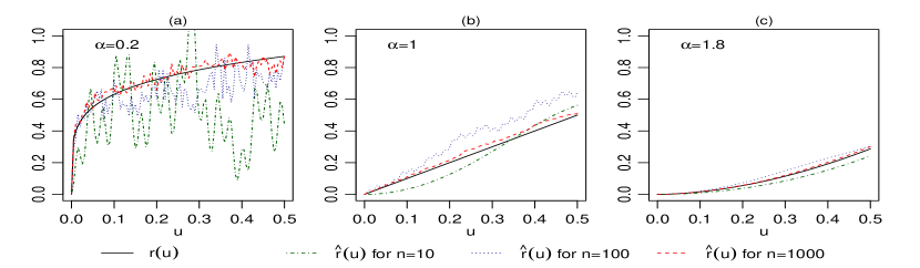
Figure 1: The values of $r(u)=u^{\alpha}$ vs $\hat{r}(u)$ of single replicates (simulated with [12]) of stable law with $\gamma=1$, $\delta=0$, $\beta=0$ for $\alpha=0.2$ in (a), $\alpha=1$ in (b) and $\alpha=1.8$ in (c) .

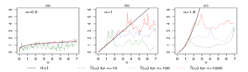
Figure 2: The values of $r(u)=u^{\alpha}$ vs $\hat{r}(u)$ of single replicates (simulated with [12]) of stable law with $\gamma=1$, $\delta=0$, $\beta=0$ for $\alpha=0.2$ in (a), $\alpha=1$ in (b) and $\alpha=1.8$ in (c) .

Figure 1 and Figure 2 show that $\hat{r}(u)$ is relatively accurate estimate of $r(u)$ only in a small interval $(0,\bar{u}]$, where $\bar{u}$ obviously depends on sample size $n$, but unfortunately also on $\alpha$ – the smaller $\alpha$, the smaller also $\bar{u}$. So, there seems not to exist an universal (that applies for any $\alpha\in(0,2]$) upper bound $\bar{u}$ so that $\sup_{u\in(0,\bar{u}]}|\hat{r}(u)-r(u)|$ were small for any $\alpha$ even when $\gamma>0$ is known. It is clearly evident from Figure 1 and Figure 2, that too big $u_{2}$ makes the estimate of $\alpha$ very imprecise. Observe that $0<u_{2}<u_{1}$ cannot also be very small, because then $\ln u_{1}-\ln u_{2}$ is also very small and that affects the preciseness of $\hat{\alpha}$ even when $\hat{r}(u_{i})\approx r(u_{i})$, $i=1,2$. On the other hand, Figure 1 and Figure 2 as well as simulations in [6] suggest that despite the possible non-existence of universal $\bar{u}$, there might exists an universal (not depending on $\alpha$ and $\gamma$) $\bar{r}$ so that $\sup_{0<u:r(u)\leq\bar{r}}|{\hat{r}}(u)-r(u)|$ is relatively small.

Our main theoretical result states that for symmetric stable laws such universal $\bar{r}$ exists.

Theorem 1.1.

Let $X_{1},\ldots,X_{n}$ be an i.i.d. sample from symmetric stable law. Fix $\epsilon>0$, $p\in(0,1)$. Then there exists $n_{o}(\epsilon,p)<\infty$ such that for every $\alpha\in(0,2]$ and $n>n_{o}$

$$P\Big{(}\sup_{0<u:r(u)\leq\bar{r}}|r(u)-\hat{r}(u)|>\epsilon\Big{)}\leq p,$$ (1.3)

where $\bar{r}(\epsilon,p,n)>0$ is independent of $\alpha$ and $\gamma$.

Theorem is proved in Subsection 2. From Theorem 1.1 it follows that with probability $1-p$, $|r(u_{i})-\hat{r}(u_{i})|\leq\epsilon$, given $n$ is big enough and $u_{i}$ is cosen such that $r(u_{i})\leq\bar{r}$, $i=1,2$. Therefore, in order to apply (1.2), it makes sense not to fix arguments $u_{1}$ and $u_{2}$, but the values $\hat{r}(u_{1})$ and $\hat{r}(u_{2})$ instead. The obtained estimate is then

$$\hat{\alpha}={\ln(\bar{r}-\epsilon)-\ln(\underline{r}+\epsilon)\over\ln u_{1}-\ln u_{2}},$$ (1.4)

where, $\epsilon$, $\bar{r}$ and $\underline{r}$ are carefully chosen constants and

$$u_{1}=\inf\{u:\hat{r}(u)=\bar{r}-\epsilon\},\quad u_{2}=\sup\{u:\hat{r}(u)=\underline{r}+\epsilon\}.$$ (1.5)

The estimates of parameters $\alpha,\beta,\gamma,\delta$ at $u_{1}$ and $u_{2}$ based on $\bar{r}-\epsilon=0.5$ and $\underline{r}+\epsilon=0.1$ were proposed and studied in [6]. The current article thus provides theoretical justification to the such method of argument selection.

Note that estimating the parameters via two points $u_{1}$ and $u_{2}$ as in (1.2) deserves more attention in the recent literature and specifying $u_{1}$ and $u_{2}$ via $\hat{r}$ function as in (1.5) is not the only option. In [1], $u_{1}=1$ and $u_{2}$ is taken such that the distance between Cauchy ($\alpha=1$) and Gaussian ($\alpha=2$) characteristic functions at $u_{2}$ were maximal. The idea of maximizing the distance between characteristic functions is further developed in [3], where an iterative 8-step algorithm for specifying $u_{1}$ and $u_{2}$ is proposed. Although the idea of maximizing discrepancy between characteristic functions (or rather between $r$-functions) is quite natural, and the simulations in [3] show good behaviour of that choice in practice, the proposed algorithm in [3] is still ad hoc in nature and lacks theoretical justification. In particular, it is not clear that it allows to choose $u_{1}$ and $u_{2}$ so that the inequality (1.6) below holds.

The proof of the Theorem 1.1 is constructive, but the goal of it is to show that universal $\bar{r}$ exists, not to optimize the constant, i.e. to find the biggest possible $\bar{r}$ and smallest possible $n_{o}$. It means that the $\bar{r}$ constructed in the proof is probably too small for practical use. Although, for every $u$, $\gamma$ and $\alpha$, $\hat{r}(u)\to r(u)$, a.s. as $n$ grows, our upper bound satisfies $\bar{r}(\epsilon,p,n)\leq w_{o}<1$, where $w_{o}$ is a constant depending on $\epsilon$. Thus $\bar{r}$ is always bounded away from 1 and does not increase to the infinity as $n$ grows. This need not necessarily be the deficiency of the proof, rather than necessary property. To see that, assume the inequality (1.3) holds with some $\bar{r}>1$. Then it follows that

$$P\Big{(}\sup_{u\in(0,\bar{u}]}|r(u)-\hat{r}(u)|>\epsilon\Big{)}\leq p,$$

where $\bar{u}=\sqrt{\bar{r}\over\gamma}$, so that the universal upper bound (that applies for any $\alpha$) $\bar{u}$ would exists. However, there is no evidence at all that such an $\bar{u}$ exists, suggesting that the a.s. convergence $\hat{r}(u)\to r(u)$ is not uniform over small $\alpha$ – for every $u$ and $n$ there exists $\alpha$ small enough so that the difference $|r(u)-\hat{r}(u)|$ is still big. If so, then $\bar{r}$ must always remain smaller than 1. The situation is different, when we bound the unknown stability parameters $\alpha$ below from zero, i.e. we assume the existence of $\underline{\alpha}>0$ (which can be arbitrary small) such that the unknown parameter $\alpha$ belongs to $[\underline{\alpha},2]$. In this case the upper bound $\bar{r}(\epsilon,p,n,\underline{\alpha})$ satisfies $\lim_{n}\bar{r}(\epsilon,p,n,\underline{\alpha})=\infty$ (Corollary 2.1), and in this case also the upper bound $\bar{u}$ exists. The existence of $\underline{\alpha}$ is common assumption in practice (e.g., [7, 4, 8] suggest $\underline{\alpha}=0.5$) and we keep this additional assumption in Theorem 2.1, that provides a uniform bound similar to (1.3) to the difference of logarithms $|\ln\hat{r}(u)-\ln r(u)|$. Theorem 2.1 is actually a simple corollary of Theorem 1.1, but the additional assumption about the existence of $\underline{\alpha}$ is necessary, because if $r$ is very small, then $|\ln\hat{r}-\ln r|$ can be rather big even when $r$ is very close to $\hat{r}$.

Section 3 is devoted to the applications of Theorem 2.1 in the light of large deviation inequalities for $\hat{\alpha}$. We show how the upper bound from Theorem 2.1 can be used to solve the two basic questions related with estimate $\hat{\alpha}$ in (1.4):

• Given precision $\epsilon_{1}>0$, probability $p$ and lower bound $\underline{\alpha}$, find $\bar{r},\underline{r},\epsilon$ (needed to construct $\hat{\alpha}$ in (1.4)) and possibly small sample size $n$ so that

  $$P\big{(}\mid\hat{\alpha}-\alpha\mid>\epsilon_{1}\big{)}\leq p.$$ (1.6)

• Given sample size $n$ and $\underline{\alpha}$, find $\bar{r},\underline{r},\epsilon$ and possibly small $\epsilon_{1}$ so that (1.6) holds. In other words, find exact i.e. non-asymptotic confidence interval to $\alpha$.

The solutions of these questions are formulated as Theorem 3.1 and Theorem 3.2.

The bound in Theorem 2.1 is constructed using the basic bound $\bar{r}(\epsilon,p,n)$ provided by Theorem 1.1. Thus the $\epsilon_{1}$ and required sample size $n$ in the inequality (1.6) depend heavily on the function $\bar{r}$. Unfortunately, the function $\bar{r}$ constructed in Section 2 is not explicitly given and, hence, difficult to work with. Although the main goal of the present paper is just to show that the function $\bar{r}$ exists, in Section 4, we discuss another possibility to construct $\bar{r}$. The new construction gives analytically more tractable bound, the price for it is bigger minimal required sample size $n_{o}$ and lower bound. Also the upper bound $\bar{r}$ constructed in Section 4 is also strictly smaller than 1 for every $n$. So we have two different constructions with the same property, and this allows us to conjecture that even the best bound $\bar{r}$ is always smaller than 1 and we also conjecture that the universal upper bound $\bar{u}$ does not exist.

Preliminaries.

For $0<\alpha<2$ every stable distribution has tail(s) that are asymptomatically power laws with heavy tails (e.g., [9, Theorem 1.12], [13, Property 1.2.15],

$$F(t) \sim c_{\alpha}\gamma^{\alpha}(1-\beta)|t|^{-\alpha},\quad\text{when }t\to-\infty,$$

$$1-F(t) \sim c_{\alpha}\gamma^{\alpha}(1+\beta)t^{-\alpha},\quad\text{when }t\to\infty,\quad$$

where $c_{\alpha}=\frac{\Gamma(\alpha)}{\pi}\sin\frac{\pi\alpha}{2}\leq\frac{1}{2}$, $\lim_{\alpha\to 0}c_{\alpha}=\frac{1}{2}$, and $\lim_{\alpha\to 2}c_{a}=0.$ For symmetric stable laws ($\beta=0$) these results imply the existence of constants $L(\alpha)$ so that

$$F(t)\leq L(\alpha)\left({|t|\over\gamma}\right)^{-\alpha},\quad\forall t<0,\quad(1-F(t))\leq L(\alpha)\left({t\over\gamma}\right)^{-\alpha},\quad\forall t>0,$$ (1.7)

Figure 3 plots the function $t\mapsto F(t){|t|}^{\alpha}$ for different $\alpha$-values and $\gamma=1$ in the range $[-5,0]$ and $[-10^{7},0]$. Increasing the interval shows similar pattern, hence it is clear that there exists $L<\infty$ so that $\sup_{\alpha\in(0,2]}L(\alpha)\leq L$. Throughout the paper, we keep $L$ undetermined, although one can take it as ${1\over 2}$. It is also obvious that $L$ is independent of $\gamma$.

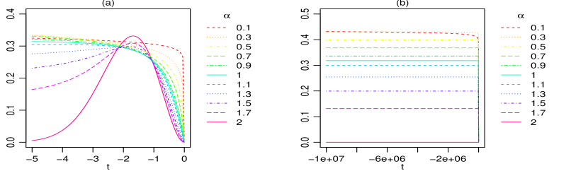
Figure 3: Plotting $t\mapsto F(t){|t|}^{\alpha}$ (calculated with [12])for different $\alpha$-values with $\gamma=1,delta=0,\beta=0$ in the range $[-5,0]$ and $[-10^{7},0]$ .

In what follows, we shall use the following elementary inequalities: for any $x,y>0$,

$$|\ln x-\ln y|\leq{|x-y|\over x\wedge y}={|x-y|\over x}\vee{|x-y|\over x-|x-y|},$$

we obtain that $|\ln x-\ln y|>\epsilon$ implies ${|x-y|\over x}>{\epsilon\over 1+\epsilon}$. Thus, for any $\bar{u}>0$ and $\epsilon>0$

$$P\big{(}\sup_{u\in(0,\bar{u}]}|r(u)-\hat{r}(u)|>\epsilon\big{)}\leq P\Big{(}\sup_{u\in(0,\bar{u}]}e^{r(\bar{u})}|\varphi(u)-\varphi_{n}(u)|>{\epsilon\over 1+\epsilon}\Big{)}.$$ (1.8)

Observe that (1.8) holds for any estimate $\varphi_{n}$.

2 Main results

2.1 Proof of Theorem 1.1

Bounding the difference of characteristic functions.

Recall $\varphi_{n}$ is the standard empirical estimate given by (1.1). To bound $|\varphi(u)-\varphi_{n}(u)|$ we use the approach in [2] as follows. For every $0<K<\infty$,

$$|\varphi_{n}(u)-\varphi(u)| =|\int e^{iux}d(F_{n}(x)-F(x))|\leq|\int_{-\infty}^{-K}e^{iux}d(F_{n}(x)-F(x))|$$

$$+|\int_{-K}^{K}e^{iux}d(F_{n}(x)-F(x))|+|\int_{K}^{\infty}e^{iux}d(F_{n}(x)-F(x))|.$$

Since $|e^{iux}|=1$ for every $u$ and $x$, the first term can be bounded

$$|\int_{-\infty}^{-K}e^{iux}d(F_{n}(x)-F(x))| \leq\int_{-\infty}^{-K}|e^{iux}|dF_{n}(x)+\int_{-\infty}^{-K}|e^{iux}|dF(x)\leq F_{n}(-K)+F(-K)$$

$$\leq\|F_{n}-F\|+2F(-K),$$

where $\|F_{n}-F\|:=\sup_{x}|F_{n}(x)-F(x)|$. The last inequality holds, because $F_{n}(-K)\leq\|F_{n}-F\|+F(-K)$. Similarly, the third term can be estimated above by $\|F_{n}-F\|+2(1-F(K))$. To estimate the second term, we use the integration by parts

$$|\int_{-K}^{K}e^{iux}d(F_{n}(x)-F(x))| =\Big{|}e^{iux}(F_{n}(x)-F(x))|_{-K}^{K}-iu\int_{-K}^{K}e^{iux}(F_{n}(x)-F(x))dx\Big{|}$$

$$\leq|F_{n}(-K)-F(-K)|+|F_{n}(K)-F(K)|+|u|\int_{-K}^{K}|F_{n}(x)-F(x)|dx$$

$$\leq 2\|F_{n}-F\|+|u|\cdot\|F_{n}-F\|\cdot 2K.$$

Therefore, for any $K$

$$|\varphi_{n}(u)-\varphi(u)|\leq 4\|F_{n}-F\|+|u|\cdot\|F_{n}-F\|\cdot 2K+2F(-K)+2(1-F(K)).$$ (2.1)

For any $\delta>0$, let $K(\delta)$ be so big that $F(-K)\leq{\delta\over 8}$. Then also $1-F(K)\leq{\delta\over 8}$ and (2.1) implies

$$|\varphi_{n}(u)-\varphi(u)|\leq{\delta\over 2}+4\|F_{n}-F\|+|u|\cdot\|F_{n}-F\|\cdot 2K(\delta).$$ (2.2)

By (1.7), we can take

$$K(\delta)=\Big{(}{8L\over\delta}\Big{)}^{1\over\alpha}{\gamma}$$ (2.3)

and so with $u>0$, by (2.2) and (2.3)

$$|\varphi_{n}(u)-\varphi(u)|\leq{\delta\over 2}+2\|F_{n}-F\|\Big{(}2+\big{(}{8Lr(u)\over\delta}\big{)}^{1\over\alpha}\Big{)}.$$ (2.4)

Bounding $r$.

Recall $\bar{r}=r(\bar{u})$. Fix $\bar{u}>0$ and define $\bar{\epsilon}=\epsilon e^{\bar{r}}$. We now use Dworetzky-Kiefer-Wolfowitz inequality [14, p. 268]):

$$P(\|F_{n}-F\|>\epsilon)\leq 2\exp[-2n\epsilon^{2}]$$

to estimate

$$P\Big{(}e^{r(\bar{u})}\sup_{u\leq\bar{u}}|\varphi_{n}(u)-\varphi(u)|>\epsilon\Big{)} \leq P\Big{(}\|F_{n}-F\|\geq{(\bar{\epsilon}-\delta/2)\delta^{1\over\alpha}\over 2\big{(}2\delta^{1\over\alpha}+(8L\bar{r})^{1\over\alpha}\big{)}}\Big{)}$$

$$=P\Big{(}\|F_{n}-F\|\geq{2^{1\over\alpha}(\bar{\epsilon}-\delta/2)({\delta\over 2})^{1\over\alpha}\over 2\big{(}2^{1+{1\over\alpha}}({\delta\over 2})^{1\over\alpha}+(8L\bar{r})^{1\over\alpha}\big{)}}\Big{)}$$

$$=P\Big{(}\|F_{n}-F\|\geq{(\bar{\epsilon}-\delta/2)({\delta\over 2})^{1\over\alpha}\over 2\big{(}2({\delta\over 2})^{1\over\alpha}+(4L\bar{r})^{1\over\alpha}\big{)}}\Big{)}$$

$$\leq 2\exp\Big{[}-{n\over 8}\cdot\Big{(}{(\bar{\epsilon}-\delta/2)({\delta\over 2})^{1\over\alpha}\over({\delta\over 2})^{1\over\alpha}+{1\over 2}(4L\bar{r})^{1\over\alpha}}\Big{)}^{2}\Big{]}.$$

Define

$$k(\alpha,\epsilon,\bar{r})={1\over 8}\Big{[}\max_{0\leq x\leq\bar{\epsilon}}{(\bar{\epsilon}-x)\over 1+{1\over 2}\big{(}{4L\bar{r}\over x}\big{)}^{1\over\alpha}}\Big{]}^{2}.$$

From (1.8), we obtain

$$P\big{(}\sup_{u\in(0,\bar{u}]}|r(u)-\hat{r}(u)|>\epsilon\big{)}\leq 2\exp[-nk\big{(}\alpha,{\epsilon\over 1+\epsilon},{\bar{r}}\big{)}]=p$$

which is equivalent to $k\big{(}\alpha,{\epsilon\over 1+\epsilon},{\bar{r}}\big{)}={\ln(2/p)\over n}$, and so the desired upper bound for any $\alpha$, denoted by $r_{n}(\alpha)$ is the solution of the following equality

$$k\big{(}\alpha,{\epsilon\over 1+\epsilon},r_{n}\big{)}={\ln(2/p)\over n}.$$ (2.5)

Observe that

$$\lim_{r\to 0}k\big{(}\alpha,{\epsilon\over 1+\epsilon},{r}\big{)}={1\over 8}\big{(}{\epsilon\over 1+\epsilon}\big{)}^{2}.$$

Hence the following condition gives a lower bound for minimal sample size $n$ so that $r_{n}(\alpha)>0$:

$$n>8\ln(2/p)\big{(}{1+\epsilon\over\epsilon}\big{)}^{2}.$$ (2.6)

The existence of $\bar{r}=\inf_{\alpha\in(0,2]}r_{n}(\alpha)$.

The following lemma shows that $\inf_{\alpha\in(0,2]}r_{n}(\alpha)>0$, hence the universal (not depending on $\alpha$ and $\gamma$) bound $\bar{r}$ exists. Since $\epsilon/(1+\epsilon)<1$, without loss of generality, in the lemma we consider $\epsilon\in(0,1)$. The lemma finishes the proof of Theorem 1.1.

Lemma 2.1.

Fix $1>\epsilon>0$ and $n$ such that $n>8{\ln(2/p)\over\epsilon^{2}}$. Let $r_{n}(\alpha)$ be the solution of the equality $k(\alpha,\epsilon,r)={\ln(2/p)\over n}$. Then $r_{n}(\alpha)$ is continuous strictly positive function on $(0,2]$ and $\lim_{\alpha\to 0}r_{n}(\alpha)>0$. In particular, $\bar{r}=\inf_{\alpha\in(0,2]}r_{n}(\alpha)>0$.

Proof.

For every $\alpha>0$ and $\epsilon>0$, define function

$$h(r,x)={(\epsilon e^{-r}-x)\over 1+{1\over 2}({4Lr\over x})^{1\over\alpha}},\quad x\in(0,\epsilon e^{-r}],\quad r>0.$$

Let us fix $r>0$ and denote $c=4Lr$. Let

$$x^{\prime}(\epsilon,r)=\arg\max_{0\leq x\leq\epsilon e^{-r}}{(\epsilon e^{-r}-x)\over 1+{1\over 2}\big{(}{c\over x}\big{)}^{1\over\alpha}}=\arg\max_{0\leq x\leq\epsilon e^{-r}}h(x,r).$$

Since $x\mapsto h(x,r)$ is continuous and strictly decreasing function, the maximizer $x^{\prime}$ exists and is unique. It is not difficult to see that $x^{\prime}$ must satisfy the following equalities:

$${(\epsilon e^{-r}-x^{\prime})\over 1+{1\over 2}({c\over x^{\prime}})^{1\over\alpha}}=\epsilon e^{-r}-(1+\alpha)x^{\prime}\quad\Leftrightarrow\quad{2\alpha\over c^{1\over\alpha}}({x^{\prime}})^{1+{1\over\alpha}}={\epsilon e^{-r}}-({1+\alpha})x^{\prime}.$$

The inequality in the left implies that

$$k(\alpha,\epsilon,r)={1\over 8}\Big{[}\sup_{x\in(0,\epsilon e^{-r}]}h(x,r)\Big{]}^{2}={1\over 8}\big{(}\epsilon e^{-r}-(1+\alpha)x^{\prime}\big{)}^{2}.$$ (2.7)

The equality in the right implies $x^{\prime}<{\epsilon e^{-r}\over 1+\alpha}$ and is equivalent to $x^{\prime}\big{(}{2\alpha\over c^{1\over\alpha}}({x^{\prime}})^{1\over\alpha}+(1+\alpha)\big{)}=\epsilon e^{-r}$. Hence we obtain

$$\epsilon e^{-r}\Big{(}{2\alpha\over c^{1\over\alpha}}\left({\epsilon e^{-r}\over 1+\alpha}\right)^{1\over\alpha}+(1+\alpha)\Big{)}^{-1}<x^{\prime}<{\epsilon e^{-r}\over 1+\alpha}.$$ (2.8)

Define function

$$f(x)=x\Big{(}{2\alpha\Big{(}{x\over c}\Big{)}^{1\over\alpha}}+(1+\alpha)\Big{)},\quad x\in(0,\epsilon e^{-r}].$$ (2.9)

Thus $x^{\prime}$ is the solution of the equality $f(x)=\epsilon e^{-r}$.

Suppose now $\alpha_{m}\to\alpha_{o}>0$. Let $f_{m}$ and $f_{o}$ be as $f$ with $\alpha_{m}$ and $\alpha_{o}$ instead of $\alpha$, respectively and let $x_{m}$ and $x_{o}$ be the solutions of the equalities $f_{m}(x)=\epsilon e^{-r}$ and $f_{o}(x)=\epsilon e^{-r}$. Clearly, for any $x\in(0,\epsilon e^{-r}]$, it holds $f_{m}(x)\to f_{o}(x)$. However, since $\alpha_{o}>0$, by (2.8) we see that there exists $y>0$ so that $x_{m}\in(y,\epsilon e^{-r}]$ eventually since obviously $\sup_{x\in[y,\epsilon e^{-r}]}|f_{m}(x)-f(x)|\to 0$, we obtain that $x_{m}\to x_{o}$ and by (2.7), thus $k(\alpha_{m},\epsilon,r)\to k(\alpha_{0},\epsilon,r)$. Now observe that for any $\alpha>0$ and $\epsilon>0$, $\lim_{r\to 0}k(\alpha,\epsilon,r)={\epsilon^{2}\over 8}$ and $\lim_{r\to\infty}k(\alpha,\epsilon,r)=0$. Moreover $r\mapsto k(\alpha,\epsilon,r)$ is strictly decreasing function. For such functions, pointwise convergence implies uniform convergence, so that as $m$ grows

$$\sup_{r\geq 0}|k(\alpha_{m},\epsilon,r)-k(\alpha_{0},\epsilon,r)|\to 0.$$ (2.10)

The uniform convergence implies that the solutions of the equalities $k(\alpha_{m},\epsilon,r)={\ln(2/p)/n}$ converge as well, i.e. $r_{n}(\alpha_{m})\to r_{n}(\alpha_{o})$, provided $n>8{\ln(2/p)\over\epsilon^{2}}$ so that the solutions exists.

We have proven that the function $r_{n}(\alpha)$ is continuous on the set $(0,2]$. Let us now consider the case $\alpha_{m}\to 0$. From the equalities $f_{m}(x_{m})=\epsilon e^{-r}$, it follows that

$$\lim_{m}x_{m}=\left\{\begin{array}[]{ll}c,&\hbox{when $c\leq\epsilon e^{-r}$;}\\ \epsilon e^{-r},&\hbox{when $c>\epsilon e^{-r}$,}\end{array}\right.$$

where $c=4Lr$. Therefore, for every fixed $r>0$,

$$k(\alpha_{m},\epsilon,r)={1\over 8}\big{(}\epsilon e^{-r}-(1+\alpha_{m})x_{m})^{2}\to k(0,\epsilon,r)$$

with

$$k(0,\epsilon,r)=\left\{\begin{array}[]{ll}{1\over 8}(c-\epsilon e^{-r})^{2},&\hbox{if $c\leq\epsilon e^{-r}\quad\Leftrightarrow\quad r\leq W({\epsilon\over 4L})$;}\\ 0,&\hbox{else,}\end{array}\right.$$

where $W$ stands for Lambert $W$-function. Observe that $r\mapsto k(0,\epsilon,r)$ is strictly decreasing function with limits $\lim_{r\to 0}k(0,\epsilon,r)={\epsilon^{2}\over 8}$ and $\lim_{r\to\infty}k(0,\epsilon,r)=0$. Hence (2.10) holds with $\alpha_{o}=0$. This, in turn, implies that $r_{n}(\alpha_{m})\to r_{n}(0)$, where $r_{n}(0)$ is the solution of the equality $k(0,\epsilon,r_{n}(0))={\ln(2/p)\over n}$. Since $\lim_{r\to 0}k(0,\epsilon,r)={\epsilon^{2}\over 8}$, and by assumption ${\epsilon^{2}\over 8}>{\ln(2/p)\over n}$, we see that $r_{n}(0)>0$. Hence $r_{n}(\alpha)$ is continuous strictly positive function on $[0,2]$, thus $\inf_{\alpha\in(0,2]}r_{n}(\alpha)>0$. ∎

2.2 Bounding $\ln r$

We are now interested in finding the probabilistic bounds on difference $|\ln r(u)-\ln\hat{r}(u)|$, where, as previously, $X_{1},...,X_{n}$ is iid sample from symmetric stable law, ${r}(u)=-\ln|\varphi(u)|=(\gamma|u|)^{\alpha}$ and $\hat{r}(u)=-\ln|\varphi_{n}(u)|$. For that an additional assumption has to be made. In the present subsection, we assume that there exists a known lower bound $0<\underline{\alpha}$ such that the parameter space is $[\underline{\alpha},2]$ instead of $(0,2]$. The crucial benefit of knowing the lower bound of $\underline{\alpha}$ is the fact that the bound $\bar{r}$ from Theorem 1.1 increases to infinity as $n$ grows. Recall that the bound $\bar{r}$ in lacks this property: although $\bar{r}$ increases with $n$, it always satisfies $\bar{r}<W({\epsilon\over 2L(1+\epsilon)})<1$ and, as argued in Introduction, such a property might be unavoidable. Bounding the parameter space away from zero, we have a new bound that tends to infinity as $n$ increases. Let us formulate it as a corollary.

Corollary 2.1.

Assume $\underline{\alpha}>0$ to be given. Fix $\epsilon>0$, $p\in(0,1)$ and let $n_{o}(\epsilon,p)<\infty$ be as in Theorem 1.1. Then for every $n>n_{o}$ there exists $\bar{r}(\epsilon,p,n,\underline{\alpha})$ independent of $\alpha$ and $\gamma$ such that $\lim_{n}\bar{r}(\epsilon,p,n,\underline{\alpha})=\infty$ and

$$P\Big{(}\sup_{u>0:r(u)\leq\overline{r}}|r(u)-\hat{r}(u)|>\epsilon\Big{)}\leq p,$$

for every $\alpha\in[\underline{\alpha},2]$ and $\gamma>0$.

Proof.

Fix $0<\underline{\alpha}<2$ and take $r_{o}$ so big that $4Lr_{o}>\epsilon e^{-r_{o}}$. Then for every $r\geq r_{o}$ and for every $x\in[0,\epsilon e^{-r}]$, the function

$$\alpha\mapsto{(\epsilon e^{-r}-x)\over 1+{1\over 2}({c4Lr\over x})^{1\over\alpha}}$$

is increasing in $\alpha$. Therefore

$$k(\alpha,\epsilon,r)\geq k(\underline{\alpha},\epsilon,r),\quad\forall\alpha\geq\underline{\alpha}\quad r\geq r_{o}.$$ (2.11)

Now observe that when $\alpha>0$, then for every $r$, it holds $x^{\prime}<{\epsilon e^{-r}\over 1+\alpha}$, thus $k(\alpha,\epsilon,r)={1\over 8}\big{(}\epsilon e^{-r}-(1+\alpha)x^{\prime})^{2}>0$. Since $\lim_{r\to\infty}k(\alpha,\epsilon,r)=0$, it follows that $\lim_{n}r_{n}(\alpha)=\infty$. Therefore, there exists $n(r_{o},\underline{\alpha})$ so big that $r_{n}(\underline{\alpha})>r_{o}$. From (2.11), it follows that when $n>n_{o}$, it holds $r_{n}(\alpha)\geq r_{n}(\underline{\alpha})$, $\forall\alpha\geq\underline{\alpha}$. Hence $\lim_{n}\inf_{\alpha\in[\underline{\alpha},2]}r_{n}(\alpha)=\lim_{n}r_{n}(\underline{\alpha})=\infty.$ The inequality in the statement now follows from Theorem 1.1. ∎

Theorem 2.1.

Assume $\underline{\alpha}>0$ to be given. Fix $\epsilon>0$, $p\in(0,1)$ and $\underline{r}>0$. Take $n_{1}(\epsilon,p,\underline{\alpha},\underline{r})$ as minimal $n$ such that

$$\bar{r}({\epsilon\over 1+\epsilon}\underline{r},p,n,\underline{\alpha})>\underline{r},\quad n_{1}(\epsilon,p,\underline{\alpha},\underline{r})\geq n_{o}({\epsilon\over 1+\epsilon}\underline{r},p),$$ (2.12)

where $n_{o}(\epsilon,p)$ is as in Theorem 1.1 and the function $\bar{r}$ is as in Corollary 2.1. Then for every $n\geq n_{1}$, $\alpha\in[\underline{\alpha},2]$ and $\gamma>0$

$$P\Big{(}\sup_{u:r(u)\in[\underline{r},\overline{r}]}|\ln r(u)-\ln\hat{r}(u)|>\epsilon\Big{)}\leq p,$$ (2.13)

where $\bar{r}=\bar{r}({\epsilon\over 1+\epsilon}\underline{r},p,n,\underline{\alpha})>\underline{r}$.

Proof.

By Corollary 2.1, such a finite $n_{1}$ exists. Now, for any $n>n_{1}$, by Corollary 2.1 again,

$$P\Big{(}\sup_{u:r(u)\in[\underline{r},\bar{r}]}|\ln r(u)-\ln\hat{r}(u)|>\epsilon\Big{)}\leq P\Big{(}\sup_{u:r(u)\in[\underline{r},\bar{r}]}|r(u)-\hat{r}(u)|>{\epsilon\over 1+\epsilon}\underline{r}\Big{)}\leq p.$$

∎

3 Applications of Theorem 2.1

Recall the estimate $\hat{\alpha}$ in (1.4). The construction of $\hat{\alpha}$ requires fixing the constants $\underline{r},\bar{r}$ and $\epsilon$. The following simple lemma shows how Theorem 2.1 can be used to prove a large deviation inequality for $\hat{\alpha}$.

Lemma 3.1.

Suppose $\underline{r}<\bar{r}$ and $\epsilon$ are chosen such that $\bar{r}-2\epsilon>\underline{r}+2\epsilon$ and (2.13) holds for some $p\in(0,1)$. Take $\epsilon_{1}>0$ so big that

$${\epsilon_{1}\over 4}\ln\left({\bar{r}-2\epsilon\over\underline{r}+2\epsilon}\right)\geq\epsilon.$$ (3.1)

Then

$$P\Big{(}|\hat{\alpha}-\alpha|\geq\epsilon_{1}\Big{)}\leq p.$$ (3.2)

Proof.

Since $u\mapsto\hat{r}(u)$ is continuous, we have by (1.4) that $\hat{r}(u_{1})=\bar{r}-\epsilon$ and $\hat{r}(u_{2})=\underline{r}+\epsilon$. Let

$$E=\big{\{}\sup_{u:r(u)\in[\underline{r},\bar{r}]}|\ln r(u)-\ln\hat{r}(u)|\leq\epsilon\big{\}}.$$ (3.3)

On the event $E$, it holds $|\hat{r}(u_{i})-r(u_{i})|\leq\epsilon$ for $i=1,2$ and so $\bar{r}-2\epsilon\leq r(u_{1})\leq\bar{r}$ and $\underline{r}\leq r(u_{2})\leq\underline{r}+2\epsilon$. Therefore, on the set $E$, for any $\epsilon_{1}>0$ the following implications hold

$$\{|\hat{\alpha}-\alpha|\geq\epsilon_{1}\} =\Big{\{}\Big{|}{\ln(\bar{r}-\epsilon)-\ln(\underline{r}+\epsilon)\over\ln u_{1}-\ln u_{2}}-{\ln r(u_{1})-\ln r(u_{2})\over\ln u_{1}-\ln u_{2}}\Big{|}>\epsilon_{1}\Big{\}}$$

$$=\big{\{}|(\ln\hat{r}(u_{1})-\ln r(u_{1}))+(\ln r(u_{2})-\ln\hat{r}(u_{2}))|>{\epsilon_{1}\ln(u_{1}/u_{2})}\big{\}}$$

$$\subseteq\big{\{}\sup_{u:r(u)\in[\underline{r},\bar{r}]}|\ln r(u)-\ln\hat{r}(u)|>{\epsilon_{1}\over 2}\ln(u_{1}/u_{2})\big{\}}$$

$$=\big{\{}\sup_{u:r(u)\in[\underline{r},\bar{r}]}|\ln r(u)-\ln\hat{r}(u)|>{\epsilon_{1}\over 2\alpha}\ln(r(u_{1})/r(u_{2}))\big{\}}$$

$$\subseteq\Big{\{}\sup_{u:r(u)\in[\underline{r},\bar{r}]}|\ln r(u)-\ln\hat{r}(u)|>{\epsilon_{1}\over 4}\ln\left({\bar{r}-2\epsilon\over\underline{r}+2\epsilon}\right)\Big{\}}.$$

We have thus shown that

$$E\cap\{|\hat{\alpha}-\alpha|\geq\epsilon_{1}\}\subseteq\Big{\{}\sup_{u:r(u)\in[\underline{r},\bar{r}]}|\ln r(u)-\ln\hat{r}(u)|>{\epsilon_{1}\over 4}\ln\big{(}{\bar{r}-2\epsilon\over\underline{r}+2\epsilon}\big{)}\Big{\}}.$$

Taking now $\epsilon_{1}$ so big that (3.1) holds, we obtain that

$$E\cap\{|\hat{\alpha}-\alpha|\geq\epsilon_{1}\}\subseteq E^{c}$$

which obviously implies that $\{|\hat{\alpha}-\alpha|\geq\epsilon_{1}\}\subseteq E^{c}$ and so (3.2) holds. ∎

Exact confidence intervals.

In what follows, we shall briefly discuss how to choose $\epsilon>0,\underline{r},\bar{r}$ such that (3.2) holds. In particular, we shall address the following classical problems of parameter estimation:

Q1:

Given lower bound $\underline{\alpha}>0$, precision $\epsilon_{1}$ and probability $p>0$, find possibly small sample size $n$ and constants $\underline{r},\bar{r},\epsilon$ (for constructing $\hat{\alpha}$) so that the estimate (1.4) satisfies inequality (3.2).

Q2:

Given lower bound $\underline{\alpha}>0$, sample size $n$ and probability $p>0$, find possibly small $\epsilon_{1}>0$ and $\underline{r},\bar{r},\epsilon$ (for constructing $\hat{\alpha}$) so that the estimate (1.4) satisfies inequality (3.2). In other words, find exact (non-asymptotic) confidence intervals: with probability $1-p$: $\hat{\alpha}-\epsilon_{1}\leq\alpha\leq\hat{\alpha}+\epsilon_{1}$.

To solve Q1, define for any $\rho>0$, $n$ and $\epsilon>0$

$$F(n,\rho,\epsilon):={\bar{r}\big{(}\rho,p,n,\underline{\alpha}\big{)}-2\epsilon\over\rho{1+\epsilon\over\epsilon}+2\epsilon}-\exp[{4\over\epsilon_{1}}\epsilon],$$ (3.4)

where $\bar{r}\big{(}\rho,p,n,\underline{\alpha}\big{)}$ is as in Corollary 2.1. The function $F$ depends also on $\underline{\alpha},\epsilon_{1}$ and $p$, but these parameters are fixed and left out from notation. Define

$$F(n,\rho)=\sup_{\epsilon>0}F(n,\rho,\epsilon),\quad F(n)=\sup_{\rho>0}\Big{[}F(n,\rho)\wedge(n-n_{o}(\rho,p))\Big{]},$$

where $n_{o}(\rho,p)$ is as in Theorem 1.1. Now take $n_{1}$ minimal $n$ such that $F(n_{1})>0$. Observe that $F(n)$ is increasing, so that when $F(n_{1})>0$, then $F(n)>0$ for any $n>n_{1}$. The estimation procedure is now the following.

EstimationProcedure1:

1. Find $n_{1}$ such that $F(n_{1})>0$.

2. Given $n\geq n_{1}$ find $\rho>0$ such that $F(n,\rho)>0$.

3. Use $\rho$ to find $\epsilon>0$ such that $F(n,\rho_{o},\epsilon)>0$.

4. Use $\rho$ to determine $\bar{r}=\bar{r}(\rho,p,n,\underline{\alpha})$, where $\bar{r}(\rho,p,n,\underline{\alpha})$ is as in Corollary 2.1.

5. Use $\epsilon$ and $\rho$ to find $\underline{r}=\rho{1+\epsilon\over\epsilon}$.

6. Use $\underline{r}$ and $\bar{r}$ to find $u_{1}$ and $u_{2}$ as in (1.5).

7. Estimate $\hat{r}(u)$ based on the sample of size $n$ and the estimate of characteristic function.

8. Find $\hat{\alpha}$ as in (1.4).

Theorem 3.1.

Let $\underline{\alpha}$, $\epsilon_{1}>0$ and $p\in(0,1)$ be given. Let $n$ be the sample size satisfying $F(n)>0$. Then the estimate $\hat{\alpha}$ obtained via EstimationProcedure1 satisfies the inequality (3.2), provided the true parameter $\alpha$ satisfies the inequality $\alpha\geq\underline{\alpha}$.

Proof.

According to definition of $F(n)$, the parameters $\rho>0$ and $\epsilon>0$ as specified by EstimationProcedure1 are such that $F(n,\rho,\epsilon)>0$ and $n>n_{o}(\rho,p)$. With $\underline{r}=\rho{1+\epsilon\over\epsilon}$, we see that

$${\bar{r}-2\epsilon\over\underline{r}+2\epsilon}>\exp[{4\over\epsilon_{1}}\epsilon]$$

so that the equation (3.1) holds. This equation also implies that $\bar{r}>\underline{r}+4\epsilon$. Since $n>n_{o}(\rho,p)$, we have $n>n_{o}({\epsilon\over 1+\epsilon}\underline{r},p)$. Thus both inequalities in (2.12) hold and therefore $n\geq n_{1}$, where $n_{1}(\epsilon,p,\alpha,\underline{r})$ is as in Theorem 2.1. Hence all assumptions of Theorem 2.1 are fulfilled and so (2.13) holds. Both assumptions of Lemma 3.1 are fulfilled and so the inequality (3.2) holds as well.∎

To solve Q2, we need to assume some minimal requirements about the given sample size $n$. In what follows, we assume that there exists $\rho_{o}>0$ such that $n>n_{o}(\rho_{o},p)$, where $n_{o}(\rho,p)$ is as in Theorem 1.1. Now we define

$$F(\epsilon_{1},\rho,\epsilon):={\bar{r}\big{(}\rho,p,n,\underline{\alpha}\big{)}-2\epsilon\over\rho{1+\epsilon\over\epsilon}+2\epsilon}-\exp[{4\over\epsilon_{1}}\epsilon].$$

The function $F(\epsilon_{1},\rho,\epsilon)$ also depends on $n$ and $p$, but these are fixed. As previously, define

$$F(\epsilon_{1},\rho):=\sup_{\epsilon>0}F(\epsilon_{1},\rho,\epsilon),\quad F(\epsilon_{1}):=\sup_{\rho\geq\rho_{o}}F(\epsilon_{1},\rho).$$

Now find (as small as possible) $\epsilon_{1}>0$ such that $F(\epsilon_{1})>0$.

EstimationProcedure2:

1. Given $\epsilon_{1}>0$ satisfying $F(\epsilon_{1})>0$ find $\rho\geq\rho_{o}$ such that $F(\epsilon_{1},\rho)>0$.

2. Use $\rho$ to find $\epsilon>0$ such that $F(\epsilon_{1},\rho,\epsilon)>0$

3. Use $\rho$ to determine $\underline{r}=\underline{r}(\rho,p,n)$, where $\bar{r}(\rho,p,n,\underline{\alpha})$ is as in Corollary 2.1.

4. Use $\epsilon$ and $\rho$ to find $\underline{r}=\rho{1+\epsilon\over\epsilon}$.

5. Use $\underline{r}$ and $\bar{r}$ to find $u_{1}$ and $u_{2}$ as in (1.5).

6. Estimate $\hat{r}(u)$ based on the sample of size $n$ and the estimate of characteristic function.

7. Find $\hat{\alpha}$ as in (1.4).

Theorem 3.2.

Let $\underline{\alpha}>0$, the sample size $n>n_{o}(\rho_{o},p)$, where $\rho_{o}>0$ and $p\in(0,1)$ be given. Let $\epsilon_{1}$ satisfy $F(\epsilon_{1})>0$. Then the estimate $\hat{\alpha}$ obtained via EstimationProcedure2 satisfies the inequality (3.2), provided the true parameter $\alpha$ satisfies the inequality $\alpha\geq\underline{\alpha}$.

Proof.

According to definition of $F(\epsilon_{1})$, the parameters $\rho>0$ and $\epsilon>0$ as specified by EstimationProcedure2 are such that $F(\epsilon_{1},\rho,\epsilon)>0$. Since $\rho\mapsto n_{o}(\rho,p)$ is decreasing, it holds that $n>n_{o}(\rho,p)$. With $\underline{r}=\rho{1+\epsilon\over\epsilon}$, we see that equation (3.1) holds. This equation also implies that $\bar{r}>\underline{r}+4\epsilon$ and hence both inequalities in (2.12) hold and therefore $n\geq n_{1}$, where $n_{1}(\epsilon,p,\underline{\alpha},\underline{r})$ is as in Theorem 2.1. Hence all assumptions of Theorem 2.1 are fulfilled and so (2.13) holds. Then Lemma 3.1 implies that (3.2) holds as well.∎

4 An alternative construction

Recall the construction of the $\bar{r}$ in the proof of Theorem 1.1: the key of the construction is the large deviation inequality

$$P\Big{(}e^{\bar{r}}\sup_{u\in(0,\bar{u}]}|\varphi_{n}(u)-\varphi(u)|>\epsilon\Big{)}\leq A\exp[-n\cdot k(\alpha,\epsilon,\bar{r})],$$ (4.1)

where $A=2$ and $k(\alpha,\epsilon,\bar{r})>0$. Then $r_{n}(\alpha)$ was defined as the solution of the equality

$$A\exp[-n\cdot k(\alpha,{\epsilon\over 1+\epsilon},r_{n})]=p$$ (4.2)

and so the the desired bound $\bar{r}=\inf_{\alpha\in(0,\alpha]}r_{n}(\alpha)$ was obtained. In order (4.2) to have positive solution, the sample size $n$ must satisfy $n>n_{o}(\epsilon,p)$. The large deviation bound (4.2) constructed in Section 2.1 is not the one possible option. We now sketch another possible construction yielding to a different inequality, and therefore, also to the different function $r_{n}(\alpha)$ and different bound $\bar{r}$. Unlike the $\bar{r}$ obtained in Section 2.1, the new $\bar{r}$ has more explicit form. The price for it is much bigger required sample sice $n_{o}$.

Observe that by (2.2) and (2.3) the inequality $\|F_{n}-F\|\leq{\delta\over 8}$ implies that

$$|\varphi_{n}(u)-\varphi(u)|\leq\delta+2\|F_{n}-F\|\Big{(}{8Lr(u)\over\delta}\Big{)}^{1\over\alpha}.$$

Hence for every $\bar{u}>0$,

$$\{e^{r(\bar{u})}\sup_{u\in(0,\bar{u}]}|\varphi(u)-\varphi_{n}(u)|>\epsilon\}\subset\{\|F_{n}-F\|>{\delta\over 8}\}\cup\Big{\{}2\|F_{n}-F\|\Big{(}{8Lr(\bar{u})\over\delta}\Big{)}^{1\over\alpha}\geq\epsilon e^{-r(\bar{u})}-\delta\Big{\}}.$$

Recall $\bar{\epsilon}=\epsilon e^{-\bar{r}}$ and $\bar{r}=r(\bar{u})$. Hence, we obtain

$$P\Big{(}e^{\bar{r}}\sup_{u\in(0,\bar{u}]}|\varphi_{n}(u)-\varphi(u)|>\epsilon\Big{)} \leq P\Big{(}\|F_{n}-F\|>{\delta\over 8}\Big{)}+P\Big{(}\|F_{n}-F\|\geq{(\bar{\epsilon}-\delta)\delta^{1\over\alpha}\over 2(8L\bar{r})^{1\over\alpha}}\Big{)}.$$

$$\leq 2\exp[-n\cdot{\delta^{2}\over 32}]+2\exp\Big{[}-n\cdot{(\bar{\epsilon}-\delta)^{2}\delta^{2\over\alpha}\over 2(8L\bar{r})^{2\over\alpha}}\Big{]}.$$ (4.3)

Choose

$$\delta={\bar{\epsilon}\over 1+\alpha}=\arg\max_{\delta\in[0,\bar{\epsilon}]}(\bar{\epsilon}-\delta)^{2}\delta^{2\over\alpha}.$$

Thus plugging $\delta$ into (4.3), we obtain with $s=2(1+{1\over\alpha})$,

$$P\Big{(}e^{\bar{r}}\sup_{u\in(0,\bar{u}]}|\varphi_{n}(u)-\varphi(u)|>\epsilon\Big{)} \leq 2\exp[-n\cdot{\bar{\epsilon}^{2}\over 32(1+\alpha)^{2}}]+2\exp\Big{[}-n\cdot\Big{(}\big{(}{\bar{\epsilon}\over 1+\alpha}\big{)}^{s}{\alpha^{2}\over 2(8L\bar{r})^{2\over\alpha}}\Big{)}\Big{]}$$

$$\leq 4\exp[-n\cdot k(\alpha,\epsilon,\bar{r})],$$

where

$$k(\alpha,\epsilon,\bar{r})=\big{(}{\epsilon^{2}e^{-2\bar{r}}\over 32(1+\alpha)^{2}}\big{)}\wedge\Big{(}{\epsilon^{s}e^{-s\bar{r}}\over 2(1+\alpha)^{s}}{\alpha^{2}\over(\bar{r}8L)^{2\over\alpha}}\Big{)}.$$

The inequality (4.2) holds with an equality, when

$${\bar{r}}=r_{1,n}(\alpha)\wedge r_{2,n}(\alpha)$$

and $r_{1,n}$, $r_{2,n}$ are solutions of the following equalities:

$$\exp[-2r_{1,n}] ={\ln(4/p)\over n}\big{(}{1+\epsilon\over\epsilon}\big{)}^{2}32(1+\alpha)^{2}$$ (4.4)

$${d(\alpha)\exp[-sr_{2,n}]\over(r_{2,n})^{2\over\alpha}} ={\ln(4/p)\over n}\big{(}{1+\epsilon\over\epsilon}\big{)}^{s},\quad\text{where }d(\alpha)={\alpha^{2}\over 2(1+\alpha)^{s}}{1\over(8L)^{2\over\alpha}}$$ (4.5)

Thus

$$r_{1,n}(\alpha)=-{1\over 2}\ln\Big{[}{\ln(4/p)\over n}\big{(}{1+\epsilon\over\epsilon}\big{)}^{2}32(1+\alpha)^{2}\Big{]}$$

and $r_{1,n}(\alpha)>0$ holds when

$$n>{\ln(4/p)}\big{(}{1+\epsilon\over\epsilon}\big{)}^{2}32(1+\alpha)^{2}.$$ (4.6)

From (4.6), we obtain necessary sample size

$$n_{o}(\epsilon,p)={\ln(4/p)}\big{(}{1+\epsilon\over\epsilon}\big{)}^{2}\cdot 288.$$ (4.7)

The solution of equality (4.5) is

$$r_{2,n}(\alpha)={1\over\alpha+1}W((\alpha+1)g_{n}(\alpha)),$$

where $W$ is Lambert’s W-function and $g_{n}$ is defined as follows

$$g_{n}(\alpha)={\alpha^{\alpha}\over 2^{\alpha\over 2}(\alpha+1)^{\alpha+1}8L}\Big{(}{n\over\ln(4/p)}\Big{)}^{\alpha\over 2}\Big{(}{\epsilon\over 1+\epsilon}\Big{)}^{\alpha+1}.$$

Observe that $\lim_{\alpha\to 0}g_{n}(\alpha)={1\over 8L}{\epsilon\over 1+\epsilon}=:g_{o}$ and $\lim_{\alpha\to 0}r_{2,n}(\alpha)=W(g_{o})\in(0,1).$ It can be shown that

$$\bar{r}(\epsilon,p,n)=\min_{\alpha}\{r_{1,n}(\alpha),r_{2,n}(\alpha)\}=\ln{\kappa}-\ln\Big{(}12\vee{\text{{${1+\alpha_{2}\over\alpha_{2}}$}}}\Big{)}>0,$$ (4.8)

where $\kappa=\frac{\epsilon}{\epsilon+1}\sqrt{{\frac{n}{2\ln(4/p)}}}$ while ${r}_{1,n}>0$ only if $\kappa>12$ and $n>n_{0}$, where $n_{o}$ is given by (4.7), and $\alpha_{2}\in(0,2]$ is the solution of the equality $r_{2,n}(\alpha)=\ln\kappa\frac{\alpha}{1+\alpha}.$

Since $\lim_{\alpha\to 0}r_{2,n}(\alpha)=W(g_{o})$, it holds that for any $n$ $\bar{r}<1$, and so the alternative construction satisfies our conjecture. However, it is possible to show the for any $\underline{\alpha}>0$,

$$\bar{r}(\epsilon,p,n,\underline{\alpha})=\inf_{\alpha\in(\underline{\alpha},2]}r_{n}(\alpha)\to\infty.$$

So we have another construction that confirms our conjecture that the universal bound $\bar{r}$ satisfies the inequality $\bar{r}<1$ and the universal bound $\bar{u}$ does not exists.

5 Comparison of $r_{n}$ and $\bar{r}$

Fix $\epsilon=0.1$, $p=0.1$ and $L=1/2$. We find the values of $r_{n}(\alpha)$ obtained in Section 2.1 as follows: first we numerically find $x^{\prime}$ as the solution of the equality $f(x)=e\mathrm{e}^{-r}$, where $f(x)$ is given by (2.9), then we calculate $k(\alpha,\epsilon,r)$ given by (2.7) and then $r_{n}$ can be found as solution of (2.5). We compare the obtained values of $r_{n}(\alpha)$ with the ones obtained in Section 4: $r_{n}(\alpha)=\min\{r_{1,n}(\alpha),r_{2,n}(\alpha)\}$, where $r_{1,n}(\alpha)$ is the solution of equality (4.4) and $r_{2,n}(\alpha)$ is the solution of equality (4.5). Note that by (4.7) we have ${r}_{1,n}(\alpha)>0$ only if $n>n_{o}\approx 128550$. Figure 4 plots both constructions of $r_{n}$ versus $\alpha\in(0.01,2]$ for different sample sizes $n$.

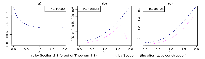
Figure 4: The values of $r_{n}$ vs $\alpha$ with $\epsilon=0.1$, $p=0.1$ and $n=1000$ in (a), $n=128551>n_{o}$ in (b) and $n=300000$ in (c).

Obviously, in Figure 4 (a) the $r_{n}(a)$ obtained by the alternative construction in Section 4 is $0$ because $n<n_{o}$. However, the values of $r_{n}$ obtained by Section 2.1 are small but positive.

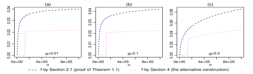
Figure 5: The values of $\bar{r}$ vs $n$ with $\epsilon=0.1$, $p=0.1$ and $\underline{\alpha}=0.01$ in (a), $\underline{\alpha}=0.1$ in (b) and $\underline{\alpha}=0.5$ in (c).

In Figure 4 (b) both constructions give positive results (because $n=n_{o}+1$) while alternative construction gives smaller (more conservative) values, with drop after $\alpha=1.5$ (and minimum over $\alpha$ is at $\alpha=2$). In Figure 4 (c) the large sample size such as $n=3\cdot 10^{5}$ is used and both $r_{n}(\alpha)$ behave in concordance while the alternative construction yields smaller values for all values of $\alpha$. Next we compare the values of $\bar{r}=\min_{\alpha\in(\underline{\alpha},2]}r_{n}(\alpha)$ obtained by Section 2.1 and Section 4. Figure 5 plots $\bar{r}$ versus $n$ for different lower limits $\underline{\alpha}$. It is clearly evident from Figure 5 that $\bar{r}$ is increasing in $n$ (while alternative construction requires $n>n_{o}$). Setting lower limit from $\underline{\alpha}=0.1$ to $\underline{\alpha}=0.5$ increases the values of $\bar{r}$ approximately twice. All in all, in our example the construction given by Section 2.1 yields much bigger (less conservative) values of $\bar{r}$ than the more explicit form construction given by Section 4.

References

- Bibalan et al. [2017] Bibalan, M. H., H. Amindavar, and M. Amirmazlaghani (2017). Characteristic function based parameter estimation of skewed alpha-stable distribution: An analytical approach. Signal Process. 130, 323–336.
- Csörgo [1981] Csörgo, S. (1981). Limit behaviour of the empirical characteristic function. The Annals of Probability 9(1), 130–144.
- Kakinaka and Umeno [2020] Kakinaka, S. and K. Umeno (2020). Flexible two-point selection approach for characteristic function-based parameter estimation of stable laws. Online at https://arxiv.org/abs/2005.11499.
- Kogon and Williams [1998] Kogon, S. M. and D. B. Williams (1998). Characteristic function based estimation of stable distribution parameters. In R. J. Adler, R. E. Feldman, and M. S. Taqqu (Eds.), A Practical Guide to Heavy Tails, pp. 311–335. Boston: Birkhäuser.
- Krutto [2016] Krutto, A. (2016). Parameter estimation in stable law. Risks 4(4), 43.
- Krutto [2018] Krutto, A. (2018). Empirical cumulant function based parameter estimation in stable laws. Acta et Commentationes Universitatis Tartuensis de Mathematica 22(2), 311–338.
- McCulloch [1996] McCulloch, J. H. (1996). Financial applications of stable distributions. In G. Maddala and C. Rao (Eds.), Statistical Methods in Finance, Volume 14 of Handbook of Statistics, pp. 393 – 425. Elsevier.
- Nolan [2001] Nolan, J. P. (2001). Maximum likelihood estimation and diagnostics for stable distributions. In O. Barndorff-Nielsen, S. Resnick, and T. Mikosch (Eds.), Lévy Processes, pp. 379–400. Boston: Birkhäuser.
- Nolan [2018] Nolan, J. P. (2018). Stable Distributions - Models for Heavy Tailed Data. Boston: Birkhäuser. In progress, Chapter 1 online at http://fs2.american.edu/jpnolan/www/stable/stable.html.
- Paulson et al. [1975] Paulson, A. S., E. W. Holcomb, and R. A. Leitch (1975). The estimation of the parameters of the stable laws. Biometrika 62(1), 163–170.
- Press [1972] Press, J. S. (1972). Estimation in univariate and multivariate stable distributions. J. Amer. Statist. Assoc. 67(340), 842–846.
- Robust Analysis Inc. [2017] Robust Analysis Inc. (2017). STABLE 5.3 R Version for Windows. Washington, DC, USA: Robust Analysis Inc. http://www.robustanalysis.com/.
- Samorodnitsky and Taqqu [1994] Samorodnitsky, G. and M. S. Taqqu (1994). Stable Non-Gaussian Random Processes: Stochastic Models with Infinite Variance. New York: Chapman & Hall.
- van der Vaart [1998] van der Vaart, A. (1998). Asymptotic Statistics. Cambridge: Cambridge University Press.
- Zolotarev [1986] Zolotarev, V. (1986). One-dimensional Stable Distributions, Volume 65 of Translations of mathematical monographs. American Mathematical Society.