Multiple metastable states in an off-lattice Potts model

Appendix A

Abstract

The interactions between a group of components are commonly studied in several areas of science (social science, biology, material science, complex dynamical systems, among others) using the methods of thermodynamics and statistical mechanics. In this work we study the properties of the recently proposed off-lattice, two-dimensional Potts model [Eur. Phys. J. B 87, 78 (2014)], originally motivated by the dynamics of agent opinions, and which is described by a Hamiltonian obtained by a maximum entropy inference procedure. We performed microcanonical and canonical Monte Carlo simulations of the first-order phase transition in the model, revealing a caloric curve with metastable regions. Furthermore, we report a “switching” behavior between multiple metastable states. We also note that the thermodynamics of the model has striking similarities with systems having long-range interactions, even though the interactions are short-ranged.

1 Introduction

Spin models, such as the Ising model and its generalization, the Potts model [1], have been proposed to describe correlation between individual sites, in different fields of Science including condensed matter physics[2], neuroscience[3], social science[4], percolation theory[5], among many others.

As is the case with several types of interacting systems presenting phase transitions, it is well known that in spin systems the phenomenon of metastability can be observed [6, 7]. A metastable state is a quasi-stable state of a dynamical system, where the macroscopic observables reach values in a steady state which, nevertheless, has a finite lifetime [8]. In the study of metastability is common the use of the microcanonical ensemble, in which we can observe precisely these forbidden states that cannot be reached within the canonical ensemble. Typical examples of metastable states are superheated solids and supercooled liquids, and in both cases the state appears at some temperatures where interesting kinetics appears. However, metastability is also observed outside the scope of thermodynamic systems, for instance in complex dynamical systems [9]. In these systems, multiple metastable states are extremely sensitive to noise or perturbations, and the initial conditions are responsible for coexistence of different attractors [10]. Moreover multistability plays an important role in some of the basic processes of life, and might even account for the maintenance of phenotypic differences in the absence of genetic or environmental distinctions [11].

In this work, we study a opinion model in social groups that takes into account how internal and external opinions may agree with each other [12]. In this model, unlike most studies on spin Hamiltonians where the spins are fixed on a lattice, we consider free-moving spins, i.e. not attached to an underlying lattice. We incorporate interactions between the agents, described by a Hamiltonian that is a variant of the two-dimensional Potts model, in which spins are free-moving particles delimited by a square box of length $L$, interacting within a radius $R_{c}$.

This paper is organized as follows. In Section 2, we define the model and its parameters, and give details on the Monte Carlo methodology used to study it, while Section 3 presents the results of a canonical and microcanonical study of first-order phase transitions in the model, together with some dynamical aspects such as multistability. Finally we close with some concluding remarks in Section 4.

2 Computational Methods

Before describing the main topic of this section, it is important to contextualize it to the social world and the interactions between individuals who might share certain opinions on a particular topic. Consider a group of $N$ individuals who interact with each other according to their $Q$ possible opinions on a subject; normally human beings can behave socially in one of two ways, namely giving an opinion according to what they truly think, or instead manifest an opinion which is not consistent with what they actually believe, in order to “fit in” better with a social group. In this work we consider individuals who are mostly consequent with their thoughts.

We will consider for our model that the opinions that agents manifest are the “spins” $S_{i}$, while in turn the agents have internal beliefs $B_{i}$, which may or may not coincide with the manifest opinion $S_{i}$ depending on the strength of the “consequence” parameter $C$. In addition, the parameter $J>0$ will play the role of an exchange coupling, which in this work can be understood as the degree of agreement among neighbors. These parameters are such that $C>J$ for the case when these agents mostly coincide their internal beliefs with the manifest opinion regardless of the external influence. On the contrary, in the case where $C<J$, internal and external opinions do not necessarily coincide, indicating that the agents are influenced by the opinions of others against their own beliefs. We will see how these two parameters arise, in the following.

The starting point of our model is the probability $p_{C}$ of having a consistent opinion, together with the probability $p_{A}$ of two agents to agree with each other given that they are closer than the radius $R_{c}$. These can be written in the form of expectation constraints as

$$P(S_{i}=B_{i}|I) =p_{C}\quad\forall\;i,$$ (1)

$$P(S_{i}=S_{j}|r_{ij}<R_{c},I) =p_{A}\quad\forall\;i,j,$$ (2)

respectively. After a maximum entropy inference [13] procedure as in Ref. [14] (see the Appendix for more details), we are led to the Hamiltonian of Ref.[12], which is given in terms of the $S_{i}$ and $B_{i}$ as follows,

$$H=-\frac{1}{2}J\sum_{i=1}^{N}\sum_{<j\neq i>}\Big{<}s_{i},s_{j}\Big{>}+\frac{1}{2}\sum_{i=1}^{N}\sum_{<j\neq i>}R-C\sum_{i=1}\Big{<}s_{i},B_{i}\Big{>},$$ (3)

where

$$\big{<}a,b\big{>}:=2\delta(a,b)-1$$

and $\delta(a,b)$ is the Kronecker delta. Note that the sum over $\big{<}j\neq i\big{>}$ term only considers the pairs within the radius $R_{c}$, which represents the extent of the influence of agents upon others.

As in Ref. [12], we are not interested in the effect of overcrowding so accordingly, the second term involving the $R$ parameter will be neglected. This is equivalent to setting $p_{A}=\frac{1}{2}$, as shown in the Appendix. So in this way and after some rearrangements, we obtain the final form of our Hamiltonian as

$$\frac{H}{C}=-\frac{1}{2}\frac{J}{C}\sum_{i=1}^{N}\sum_{<j\neq i>}\delta(s_{i},s_{j})\Theta(Rc-r_{ij})-2\sum_{i=1}\delta(s_{i},B_{i}).$$ (4)

For clarity, we will take $C$=1 and express the results in terms of the ratio $J/C$, while also using $C$ as the unit of energy. A given value of $J/C$ can be understood as a degree of tendency to belong to a group by maintaining or changing their opinion, depending on its value. In this case we consider a positive value of $J/C<1$, which means an agent will tend to remain firm with his inner opinion and would tend to leave a group.

Please also note that the Hamiltonian as given by Eq. 4 involves only the configurational degrees of freedom $S_{i}$ and $\bm{r}_{i}$, and therefore represents the potential energy of the system. Accordingly, in the following we will denote this part as $\Phi$. Furthermore, potential energy in this model is higher if pairs of agents with the same manifest opinion are farther than $R_{c}$ due to the interaction parameter $J$, and also higher if the agents manifest a different opinion than their internal belief, because of the consequence parameter $C$.

2.1 Monte Carlo Metropolis algorithm

In order to determine the properties of this model, we have performed microcanonical and canonical ensemble simulations using in the former case Ray’s version of the Monte Carlo Metropolis algorithm [15].

For the canonical ensemble, as is well known[16] the acceptance probability is given by

$$p_{\text{acc}}=\min\big{(}1,\exp{(-\beta\Delta\phi)}\Big{)}$$ (5)

while in the microcanonical ensemble, it is given by

$$p_{\text{acc}}=\min\Big{(}1,\Big{[}\frac{E-\Phi^{\prime}}{E-\Phi}\Big{]}^{\frac{dN}{2}-1}\Big{)}$$ (6)

where $d$ is the dimension of the system, and in our case $d=2$. Finally we obtain

$$p_{\text{acc}}=\min\Big{(}1,\Big{[}\frac{E-\Phi^{\prime}}{E-\Phi}\Big{]}^{N-1}\Big{)}.$$ (7)

The Monte Carlo trial moves used for this work were considered under two conditions, regarding a probability $p_{s}$ for particles to change spin, or otherwise, move and interact with other agents. More precisely, if a uniform random variable $x\in[0,1)$ is such that, $x<p_{s}$ then a previously selected agent appears to “change its mind”, that is, changes its spin. If, on the other hand, $x\geq p_{s}$ the selected agent does not change opinion. Instead, it changes position and, in doing so may interact with other agents. In our work we used a value $p_{s}$=0.1.

The temperature in the microcanonical ensemble $T(E)$ is obtained from the configurations by the relation [17]

$$\frac{1}{T(E)}:=\Big{<}\frac{dN}{2(E-\Phi)}\Big{>}_{E}=\Big{<}\frac{N}{(E-\Phi)}\Big{>}_{E}.$$ (8)

3 Results

As was shown in Ref.[12], the model has both second-order and first-order phase transitions depending on the values of $\rho:=R_{c}/L$ and $J/C$. In this study we have chosen to focus our attention on the first-order phase transitions and the presence of metastable states. Therefore, for our simulations using the Monte Carlo Metropolis algorithm we have used the two-dimensional $Q$=2 Potts model case, with a particle number $N$=100, where the values of parameters used are $\rho$ = 0.06, $J/C$ = 0.6 and $R_{c}$ = 6.708, in all cases which are different as in [12], in the same way we made this simulation considering a square box of side $L$=111.8 units, which is proportional to $N$.

3.1 Canonical and microcanonical thermodynamics of the model

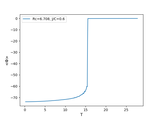
Figure 1: Caloric curve for the canonical ensemble, where a first-order phase transition can be seen. The y-axis show the expectation value of Potential Energy $\big{<}\Phi\big{>}$.

Fig. 1 shows the canonical caloric curve $\big{<}\Phi\big{>}_{\beta}$ versus $T$, in which at low energies (approaching $\big{<}\Phi\big{>}$ = -60 from below), small perturbations can be seen due to being close to the critical point $T_{c}$ = 15.5 where the phase transition occurs. Similarly, Fig. 2 shows the microcanonical caloric curve $\big{<}T\big{>}_{E}$ versus $E$ where this kind of perturbation is seen in greater detail, as well as the phase transition that in the caloric curve of the canonical ensemble is an abrupt vertical curve. The microcanonical caloric curve strikingly resembles those of systems with long-range interactions [18, 19], despite the fact that our model only consider direct interactions within the cutoff $R_{c}$.

Figure 2: Caloric curve for the microcanonical ensemble, where a first-order phase transition, together with a region of metastability, can be seen.

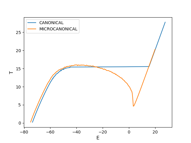
Figure 3: Cross curves between Microcanonical and Canonical Ensemble

In Fig. 3 the crossing curves represent the microcanonical caloric curve of Fig.2 superimposed with the canonical caloric curve of Fig.1 but where in the latter we have added the kinetic energy $\big{<}K\big{>}_{\beta}=N/\beta$. We can observe an interesting situation, namely the presence of metastable states between the equilibrium, stable branches (straight lines) below $E$ = -60 and above $E$ = 20. A large metastable region appears clearly between the intersections of the canonical and microcanonical curves at $E$=-25.6525 and $E$=15.2448.

3.2 Metastable states

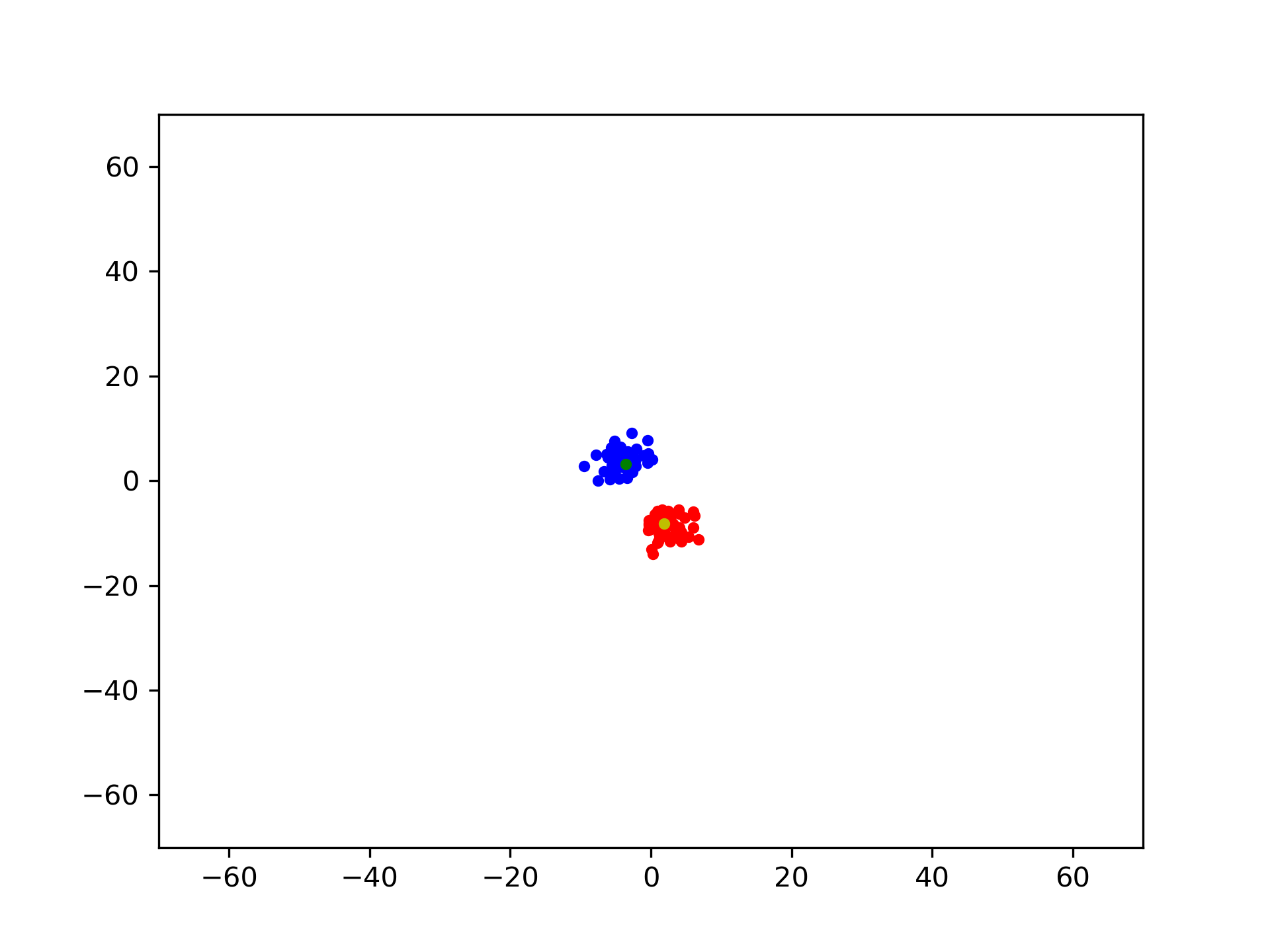
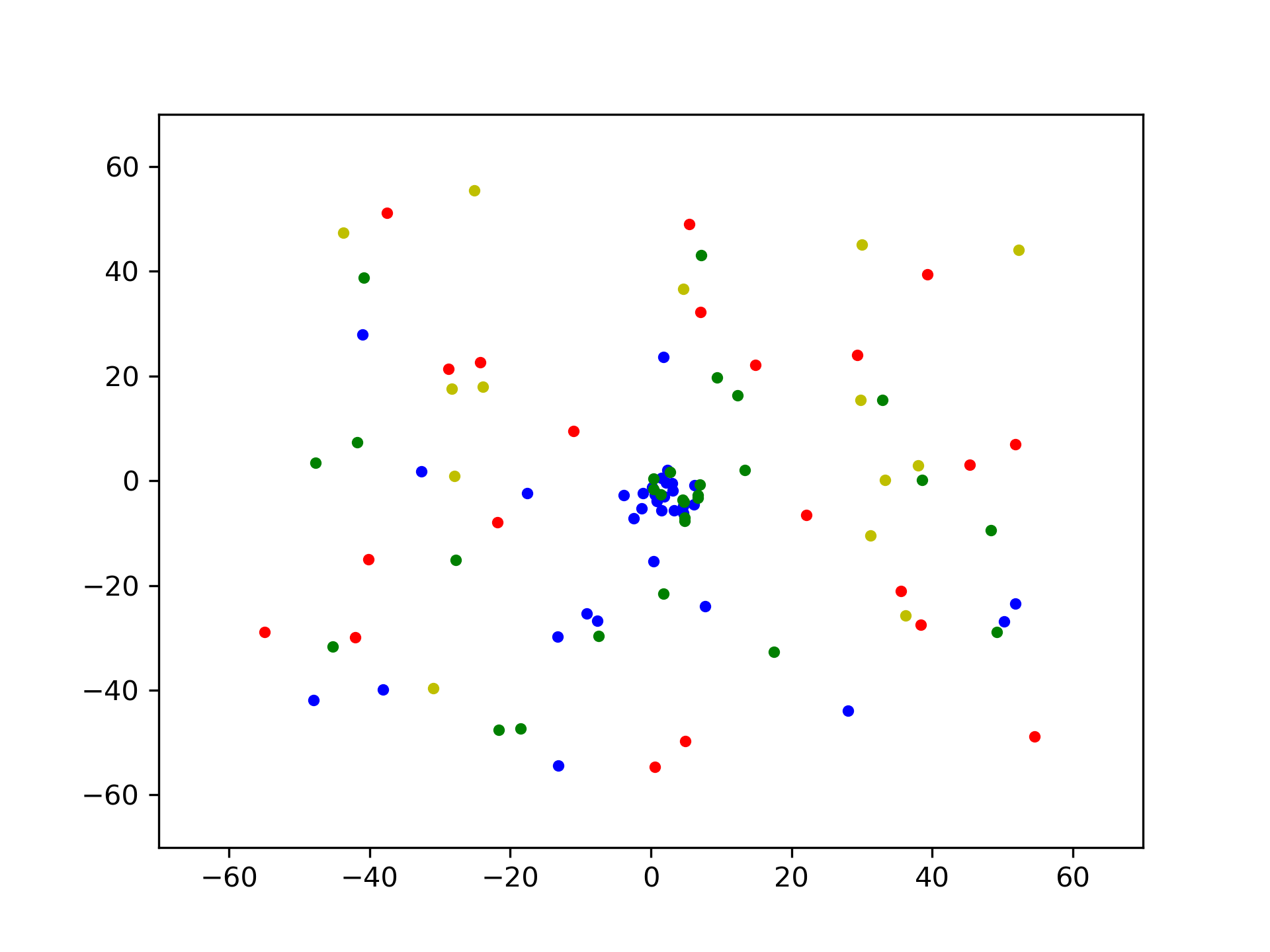
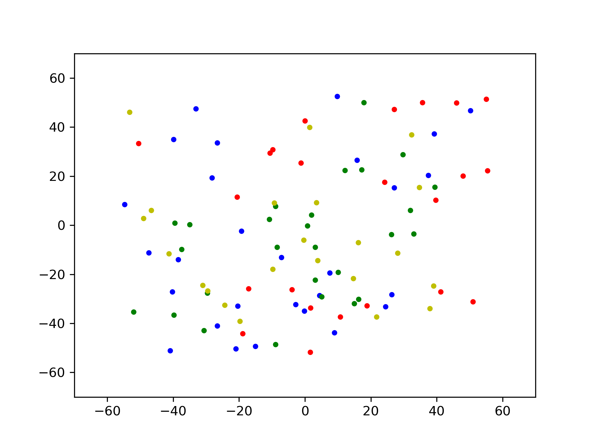
Figure 4: Dynamics in stable and metastable zones. The left-side image shows a single-cluster; the center shows the main cluster and the right-side image show the cloud of stable states. Each of these images shows four different configurations of $S_{i}$ and $B_{i}$; where: blue points refer to $S_{i}=0$ and $B_{i}=0$; red points when $S_{i}=1$ and $B_{i}=1$; green points when $S_{i}=0$ and $B_{i}=1$ and finally yellow points when $S_{i}=1$ and $B_{i}=0$.

As is well known, in a first-order phase transition we normally have two clearly distinct states that can be seen in a caloric curve as in Fig. 1, in which we only observe a low-energy and a high-energy state separated by a gap. The nature of these stable states can be understood by thinking in terms of the solid-liquid phase transition, where the particles are together at low energies and without being disturbed, in a state of thermodynamic equilibrium. On the other hand, at higher energies the particles are separated and move independently, reaching a new state of equilibrium where they do not interact with each other as much, and that is what we call the liquid phase.

However, metastable states are transient states located outside the equilibrium region of the phase diagram, that are not accesible from the canonical ensemble. A typical example of metastable state it the superheated liquid state which, when being perturbed, spontaneously reaches the gaseous state. More closely related to our model is the Hamiltonian Mean Field (HMF) model, which is useful as a model system to study long-range interactions, and which presents metastable states [20, 21].

In order to gain some insight into the behavior of agents in their stable and metastable states, Fig.4 shows three snapshots of the agents configuration at different energies, $E$=-30.0 (left), $E$=3.0 (center) and $E$=20.0 (right), where in each of the panels a particular collective behavior can be seen. In all cases the dynamics begins with an initial configuration of two groups separated by a distance larger than $R_{c}$ so that they do not interact with each other. These groups are shown as blue ($S=B=0$) and red ($S=B=1$) points. It corresponds to the ground state of the system.

In the first zone, at low energies, we have two clusters of agents where each group is mostly consistent with their beliefs, while a few on each cluster only belongs to the cluster by manifesting a false opinion. These correspond to the green points ($S=0$ and $B=1$) in the blue group and the yellow points ($S=1$ and $B=0$) in the red group.

In the second zone we have metastability, and in this case some of the agents look for others who have the same opinion (even if they have to “fake” said opinion) and form a main cluster that is, a group of people who interact and talk about a particular topic), while the rest do not agree and they move away to form a kind of “cloud”. Finally, at high energies ($E>5$ units) we have a stable state where only the “cloud” exists: the agents barely interact and these individuals can be interpreted as being detached from both their own beliefs and the opinion of others.

In both the caloric curves and the configurations of the particles (agents), we see striking similarities with the self-gravitating ring (SGR) model by Casetti and Nardini [18], despite the fact that in our model the interactions are short-ranged.

It is common for metastable states to manifest interesting dynamical properties, such as anomalous diffusion [22, 23]. For instance, the superheated solid constitutes a metastable state where a cooperative mobility appears when the energy is incremented [24, 25, 26]. In our case we also expect to have cooperative mobility because of the abrupt nature of the transition between cluster and cloud, but is probably given according to interactions due to the four different configurations as we have described.

3.3 Stochastic dynamics and multistability

We have also explored the stochastic dynamics ocurring in the system in these microcanonical metastable states [27]. Figs. 5 and 6 show a phenomenon of dynamical multistability near the higher energy transition point at $E$=3, which is similar to the oscillation of phases that ocurrs for small systems near a first-order phase transition [28, 6] and have been also reported previously in complex dynamical systems [29].

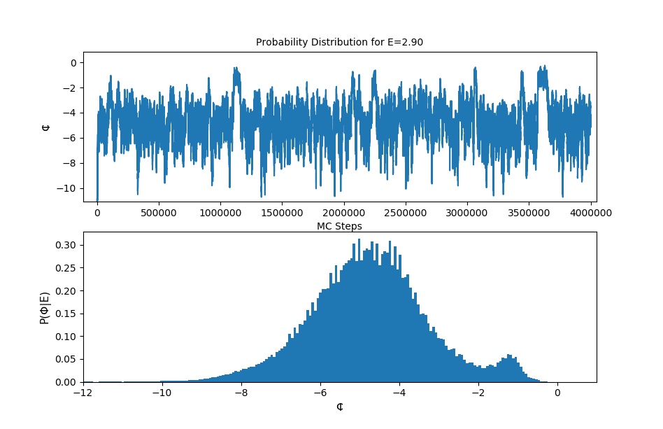
Figure 5: Left panel, trace plot (above) of potential energy $\Phi$ during 4 million Monte Carlo steps, and its histogram (below) for $E$=2.90. Right panel, trace plot (above) of potential energy $\Phi$ during 4 million Monte Carlo steps, and its histogram (below) for $E$=3.006125.

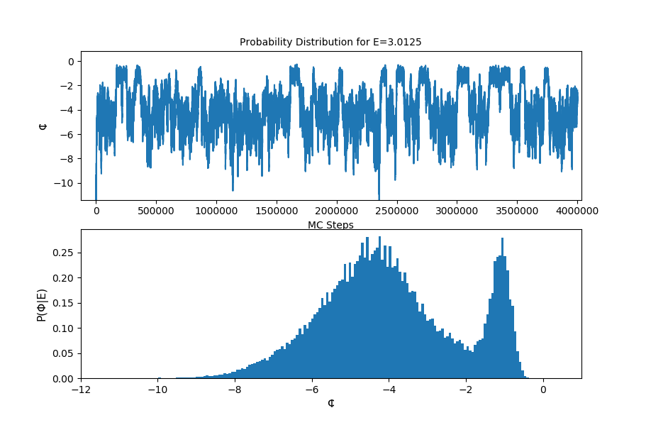
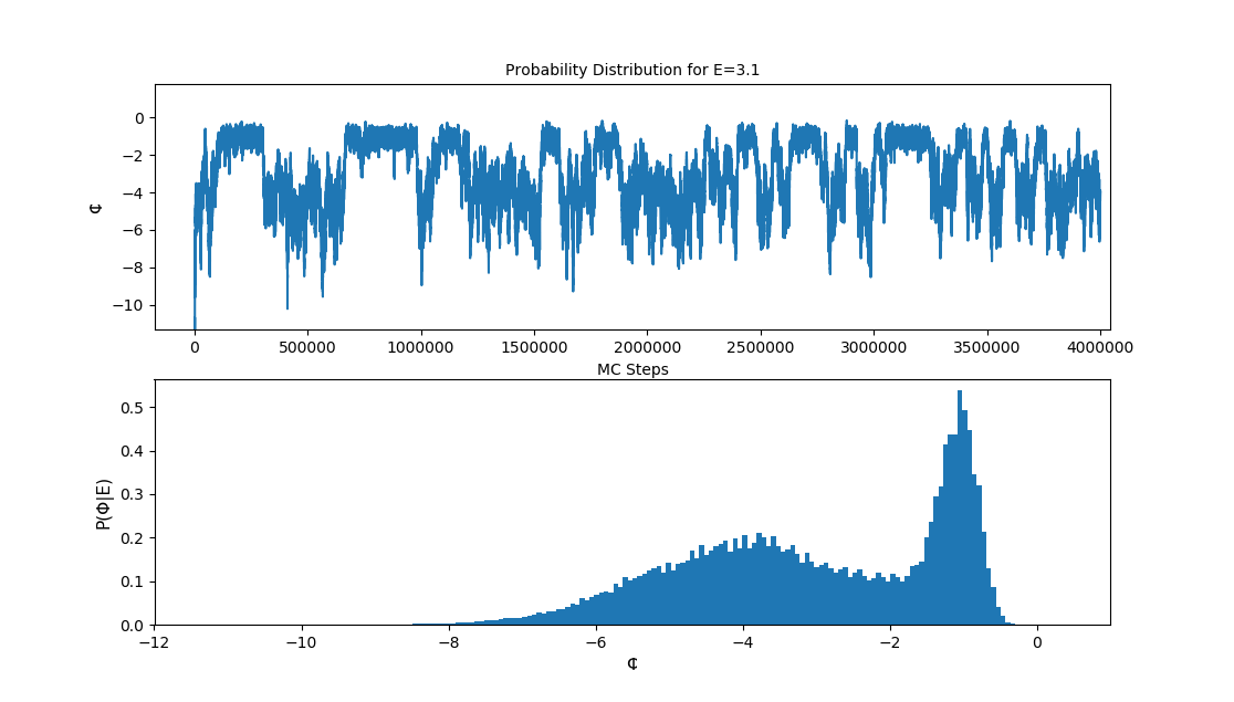
Figure 6: Left panel, trace plot (above) of potential energy $\Phi$ during 4 million Monte Carlo steps, and its histogram (below) for $E$=3.0125. Right panel, trace plot (above) of potential energy $\Phi$ during 4 million Monte Carlo steps, and its histogram (below) for $E$=3.1.

We see in the left panels of Fig. 5 a distribution that begins to have a bimodal shape, while most of the distribution is concentrated in the first peak, which according to Fig. 2 at this energy is a stable configuration. However, in the right panel it is shown that there are more clear signs of a bimodal distribution, and this is due to an increase in total energy, which favors the higher potential energy state (above -2 units). It is well-known that metastable states present bimodal distributions of total energy (in the canonical ensemble) and potential energy (in the microcanonical ensemble). In the latter case, as a consequence of the shape of the microcanonical caloric curve, indicating a coexistence of phases [30].

In Fig. 6, two other sequential panels are shown with increasing energy and maintaining a bimodal distribution but in these cases more pronounced in the secondary peak; rather, the distribution shifts according to the fact that the states tend to stay at one of the potential energy minima for a certain time until they spontaneously switch to another. These metastable states have usually short lifetimes, but can last a considerable proportion of the total simulation time. In the right panel of Fig. 6, we see that for a higher energy, the secondary peak has the highest density and this means that it has become the most stable state. These simulation results suggest a transition energy at $E\sim 3.006125$. Additionally, Figs. 5 and 6 also suggest the appearance of multiple metastable states close to one another. The dynamics that are observed are strongly dependent on the particular initial conditions imposed [21], since they determine the local minimum the system is closest to at the beginning.

4 Concluding Remarks

In summary, we have presented canonical and microcanonical simulations of an off-lattice variant of the Potts model which arises from a maximum entropy inference procedure, where agents move freely and interact depending of their opinions, under one of four different possible configurations for $Q$=2. Given that $B\in\{0,1\}$ we have two combinations with $S=B$, corresponding to an agent manifesting a consistent opinion, and two combinations with $S\neq B$, where the agent expresses an opinion contrary to its internal belief.

This variant of the Potts model presents a first-order phase transition with multiple metastable states which appear on a V-shaped region of the caloric curve with negative specific heat, between $E=-25.6525$ and $E=15.2448$ in Fig.3.We have presented the dynamics of this system in a graphical way in three different zones, namely “two clusters”, “main cluster plus cloud” and “cloud”, in which the main cluster plus cloud configuration is clearly a metastable state that is forbidden in the canonical ensemble.

The dynamical phenomenon of multistability, being a common phenomenon in complex dynamical systems, is also present in our case as the system explores the metastable states (local minima) on both sides of a bimodal distribution of potential energy in the V-shaped region. These states have short lifetimes, and the system oscillates frequently between the different local minima. In this work we have presented a system with short-range interactions in which surprisingly there is a similar behavior to a long-range interacting system. This last result is interesting for future work related to this type of interacting spin models.

5 Acknowledgements

SD gratefully acknowledges partial funding from FONDECYT 1171127 and Anillo ACT-172101 grants.

Appendix A Derivation of the model

In this section we show the mathematical development of the main model used in this work. We start from the constraints

$$P(S_{i}=B_{i}|I)=\Big{<}\delta(S_{i},B_{i})\Big{>}_{I} =p_{c}\qquad\forall i=1,i\ldots,N$$ (9)

$$P(S_{i}=S_{j}|r_{i,j}<R_{c},I)=\frac{\Big{<}\delta(S_{i},S_{j})\Theta(R_{c}-r_{i,j})\Big{>}_{I}}{\Big{<}\Theta(R_{c},r_{i,j})\Big{>}_{I}} =p_{A}\qquad\forall i,j=1,\ldots,N$$ (10)

The constraint in equation (10) can be written as

$$\Big{<}\Theta(R_{c},r_{i,j})(\delta(S_{i},S_{j})-p_{A})\Big{>}_{I}=0\qquad\forall i=1,\ldots,N$$ (11)

Maximizing the Shannon entropy under the constraints in Eqs. 9 and 10, the model is

$$P(S_{1},...,S_{N}|B_{1},...,B_{N},I)=\frac{1}{Z}\exp\Big{(}-\sum_{i=1}^{N}\lambda_{i}\delta(S_{i},B_{i})-\sum_{i=1}^{N}\sum_{j=1}^{N}\mu_{ij}\Theta(R_{c}-r_{ij})(\delta(S_{i},S_{j}-p_{A}))\Big{)}$$ (12)

which resembles a canonical ensemble. Therefore, after assuming $\lambda_{i}=\lambda$ and $\mu_{ij}=\mu$ we can write Eq. 12 as

$$P(S_{1},\ldots,S_{N}|B_{1},\ldots,B_{N},I):=\frac{1}{Z}\exp(-\beta H(S_{1},\ldots,S_{N};B_{1},\ldots,B_{N},\lambda,\mu))$$ (13)

with the definition of a Hamiltonian

$$H=-C\sum_{i=1}^{N}\Big{<}s_{i},B_{i}\Big{>}-CN-\frac{1}{2}J\sum_{i=1}^{N}\sum_{<j\neq i>}\Big{<}s_{i},s_{j}\Big{>}+\frac{R}{2}\sum_{i=1}^{N}\sum_{<j\neq i>}1,$$ (14)

where $\big{<}a,b\big{>}:=2\delta(a,b)-1$ and with the new parameters

$$C :=-\frac{\lambda}{2\beta}$$ (15)

$$J :=-\frac{\mu}{\beta}$$ (16)

$$R :=J(2p_{A}-1).$$ (17)

The choice $p_{A}=\frac{1}{2}$ eliminates the overcrowding term, and the constant term $-CN$ is absorbed into the normalization factor, i.e. the partition function.

References

- [1] F. Y. Wu. The Potts model. Rev. Mod. Phys., American Physical Society, 54:235–268, 1982.
- [2] D Louis, D Lacour, M Hehn, V Lomakin, Thomas Hauet, and F Montaigne. A tunable magnetic metamaterial based on the dipolar four-state Potts model. Nature Materials, 17(12):1076–1080, 2018.
- [3] M. Naim et al. Reducing a cortical network to a potts model yields storage capacity estimates. J. Stat. Mech., 2018(4):043304, 2018.
- [4] C. Bisconti, A. Corallo, L.Fortunato, A. Gentile, A. Massafra, and P. Piergiuseppe. Reconstruction of a real world social network using the potts model and loopy belief propagation. Front Psychol., 6:1968, 2015.
- [5] P. Debenedetti and F. Stillinger. Supercooled liquids and the glass transition. Nature, 410:259–267, 2001.
- [6] F. Moreno, S. Davis, C. Loyola, and J. Peralta. Ordered metastable states in the Potts model and their connection with the superheated solid state. Phys. A, 509:361–368, 2018.
- [7] M. Nishino, P. Rikvold, C. Omand, and S. Miyashita. Multistability in an unusual phase diagram induced by the competition between antiferromagnetic-like short-range and ferromagnetic-like long-range interactions. Phys. Rev. B, 98:144402, 2018.
- [8] M.S. Shell. Thermodynamics and Statistical Mechanics: An Integrated Approach. Cambridge Series in Chemical Engineering. Cambridge University Press, 2015.
- [9] G. Zeng, J. Gao, L. Shekhtman, S. Guo, W. Lv, J. Wu, H. Liu, O. Levy, D. Li, Z. Gao, H. E. Stanley, and S. Havlin. Multiple metastable network states in urban traffic. Proceedings of the National Academy of Science, page 201907493, 2020.
- [10] U. Feudel. Complex dynamics in multistable systems. International Journal of Bifurcation and Chaos, 18:1607–1626, 2008.
- [11] M. Laurent and N. Kellershohn. Multistability: a major means of differentiation and evolution in biological systems. Trends in biochemical sciences, 24(11):418–422, 1999.
- [12] S. Davis, Y. Navarrete, and G. Gutiérrez. A maximum entropy model for opinions in social groups. Eur. Phys. J. B, 87:78, 2014.
- [13] E. T. Jaynes. Information theory and statistical mechanics. Phys. Rev., 106:620, 1957.
- [14] M. Castellana and W. Bialek. Inverse spin glass and related maximum entropy problems. Phys. Rev. Lett., 113:117204, 2014.
- [15] J. R. Ray. Microcanonical ensemble monte carlo method. Phys. Rev. A, 44:4061–4064, 1991.
- [16] J. Tobochnik and H. Gould. Teaching statistical physics by thinking about models and algorithms. Am. J. Phys., 76:353, 2008.
- [17] M. A. Carignano. Monte carlo simulations of small water clusters: microcanonical vs canonical ensemble. Chem. Phys. Lett., 361:291–297, 2002.
- [18] L. Casetti and C. Nardini. A solvable model of a self-gravitating system. J. Stat. Mech.: Theory and Experiment, 2010:P05006, 2010.
- [19] L. Casetti and C. Nardini. Caloric curve of star clusters. Phys. Rev. E., 85:061105, 2012.
- [20] T. Dauxois, V. Latora, and A. Rapisarda. The Hamiltonian Mean Field model: From dynamics to statistical mechanics and back. Springer, 602, 2002.
- [21] B. Atenas and S. Curilef. Dynamics and thermodynamics of systems with long-range dipole-type interactions. Phys. Rev. E, 95:022110, 2017.
- [22] C. Klix, C. Patrick Royall, and H. Tanaka. Structural and dynamical features of multiple metastable glassy states in a colloidal system with competing interactions. Phys. Rev. Letters, 104:165702, 2010.
- [23] I. M. Sokolov. Models of anomalous diffusion in crowded environments. Soft Matter, 8:9043, 2012.
- [24] S. Davis, A. B. Belonoshko, B. Johansson, and A. Rosengren. Model for diffusion at the microcanonical superheating limit from atomistic computer simulations. Phys. Rev. B, 84:64102, 2011.
- [25] H. Zhang, M. Khalkhali, Q. Liu, and J. F Douglas. String-like cooperative motion in homogeneous melting. J. Chem. Phys., 138:12A538, 2013.
- [26] V. Olguín-Arias, S. Davis, and G. Gutiérrez. Extended correlations in the critical superheated solid. J. Chem. Phys., 151:064507, 2019.
- [27] Two animations of the dynamics for the case E=-0.5 can be found at http://lpmd.cl/sdavis/potts_anim_Em0.5_v1.mp4 and http://lpmd.cl/sdavis/potts_anim_Em0.5_v2.mp4.
- [28] D. Alfè, C. Cazorla, and M.J Gillan. The kinetics of homogeneous melting beyond the limit of superheating. J. Chem. Phys., 135:24102, 2011.
- [29] K. Sneppen and N. Mitarai. Multistability with a metastable mixed state. Phys. Rev. Lett., 109:100602, 2012.
- [30] M. Eryürek and M.H. Güven. Negative heat capacity of Ar55 cluster. Physica A, 377:514–522, 2007.