Gate-free state preparation for fast variational quantum eigensolver simulations

Abstract

The variational quantum eigensolver (VQE) is currently the flagship algorithm for solving electronic structure problems on near-term quantum computers. This hybrid quantum/classical algorithm involves implementing a sequence of parameterized gates on quantum hardware to generate a target quantum state, and then measuring the expectation value of the molecular Hamiltonian. Due to finite coherence times and frequent gate errors, the number of gates that can be implemented remains limited on current quantum devices, preventing accurate applications to systems with significant entanglement, such as strongly correlated molecules. In this work, we propose an alternative algorithm (which we refer to as ctrl-VQE) where the quantum circuit used for state preparation is removed entirely and replaced by a quantum control routine which variationally shapes a pulse to drive the initial Hartree-Fock state to the full CI target state. As with VQE, the objective function optimized is the expectation value of the qubit-mapped molecular Hamiltonian. However, by removing the quantum circuit, the coherence times required for state preparation can be drastically reduced by directly optimizing the pulses. We demonstrate the potential of this method numerically by directly optimizing pulse shapes which accurately model the dissociation curves of the hydrogen molecule (covalent bond) and helium hydride ion (ionic bond), and we compute the single point energy for LiH with four transmons.

I Introduction

Molecular modeling stands in the juncture of key advances in many important fields including and not limited to energy storage, novel material designs, and drug discovery. For more than half a century, many seminal works have been reported on the development of theories and methods to enable molecular modeling with high accuracies. Approximate numerical methods which are built on a single Slater determinant reference state, such as density functional theory (DFT), perturbation theory, or coupled cluster, perform well when the amount of electron correlation, ranges from minimal to moderate. However, for systems which are qualitatively governed by electron correlation effects (strongly correlated systems), such approximate methods fail to be sufficiently accurate. While alternative strategies exist, such as density matrix renormalization group (DMRG)White (1992); Chan and Head-Gordon (2002); Schollwöck (2011) or selected configurational interaction (SCI) methods,Huron et al. (1973); Bender and Davidson (1969); Buenker (1968); Evangelisti et al. (1983); Tubman et al. (2016); Schriber and Evangelista (2016); Holmes et al. (2016); Levine et al. (2020); Abraham and Mayhall (2020); Caffarel et al. (2016) which can handle strong correlation, these approaches assume that the correlations are either low-dimensional, or limited in scale. Currently, no polynomially scaling classical algorithm exists which can solve for arbitrary molecular ground states.

High dimensionality of the wavefunction is ultimately the core reason for the exponential cost of modeling electronic structure. Even before optimization, simply storing the wavefunction on classical hardware quickly becomes a bottleneck. This is because one typically represents the wavefunction in a basis of “classical” states, or basis states which have a direct product structure (Slater determinants, occupation number vectors, or even tensor product statesAbraham and Mayhall (2020)). In this classical basis, the exact (and generally entangled) state of the system is represented as an exponentially large vector of coefficients weighting the corresponding classical basis states.

Quantum computing offers a radical departure from this computational strategy. As quantum systems themselves, the state of a quantum processing unit (QPU) is also a vector in a Hilbert space of identical dimension to the molecular problem. This ability to perform a one-to-one mapping between vectors in the Hilbert space containing the molecule’s electronic wavefunction and those in the state space accessible to a QPU means that with enough control over the QPU, it should be possible to take the vector corresponding to the molecular wavefunction and realize it on the QPU, avoiding altogether the requirement to work with an exponentially large vector of coefficients. Once the QPU is prepared into the state corresponding to the target molecule, any molecular observable (energy, dipole moment, etc) can be obtained by measuring the corresponding operator on the QPU.

In order to turn this strategy into an algorithm, one needs a procedure for realizing the target molecular wavefunction on the QPU. As the leading quantum algorithm for molecular simulation on near-term devices, the Variational Quantum Eigensolver (VQE)Peruzzo et al. (2014) provides an efficient procedure for this purpose. In VQE, one defines a parameterized quantum circuit comprised of tunable gates, and then optimizes these gates using the variational principle, minimizing the energy of the molecular Hamiltonian. This parameterized quantum circuit (referred to as an ansatz) defines the variational flexibility (and thus the subspace reachable on the QPU) of the algorithm.

State-preparation circuits with more parameters generally have more variational flexibility, but come with the cost of having deeper quantum circuits and more difficult optimization. This cost can be significant. Current and near-term quantum computers are classified as noisy intermediate scale quantum (NISQ) devices due to the presence of short coherence times, system noise, and frequent gate errorsPreskill (2018). Because each gate has limited fidelity, the success probability for a sequence of gates decreases exponentially with circuit depth. Even if gates could reach unit fidelity, the finite coherence times of a NISQ device still limits the number of gates that one can apply in a circuit which, in turn, limits the accuracy of the molecular VQE simulation. Although VQE is relatively robust in the presence of noise and errors in certain cases,Sharma et al. (2020) the critical limitation preventing larger scale experiments is the accurate implementation of deep circuits. The goal of finding parameterized circuits which minimize the circuit depth and maximize the accuracy has led to a number of approaches such as hardware efficient ansätze,Kandala et al. (2017) physically motivated fixed ansätze,Huggins et al. (2019a); Lee et al. (2019); Gard et al. (2020); Barron et al. (2020a); Ryabinkin et al. (2018) and adaptive ansätze.Grimsley et al. (2019); Tang et al. (2020); Ryabinkin et al. (2020)

Each of these mentioned approaches essentially aims to find the shortest quantum circuit for preparing a state to within an acceptable error. However, even if one succeeds at finding the “best” circuit, it is likely that its execution time will still exceed the coherence time of a NISQ device. In order to make meaningful progress toward larger problems, one can imagine three strategies: (i) device improved error mitigation techniques, (ii) significantly increase the ratio of coherence to gate time, or (iii) simply abandon gates and directly optimize the electronic controls. Of these, the latter strategy appears to be the most feasible on near-term NISQ devices.

In this paper, we explore the possibility of performing gate-free VQE simulations by replacing the parameterized quantum circuit with a direct optimization of the laboratory-frame analogue control settings. In the following sections, we argue that quantum control techniques are likely to be better suited for fast VQE state preparation than the more conventional circuit-based approaches on NISQ devices. We first provide a detailed overview of circuit-based VQE, then introduce our proposed strategy, ctrl-VQE, then discuss initial results along with a strategy to avoid over-parameterization, and finally compare to gate-based ansätze. Several technical aspects, numerical results, and additional discussion are provided in the supplementary information.

II Method

II.1 Variational Quantum Eigensolver

The VQE algorithm aims to leverage classical resources to reduce the circuit depth required for molecular simulation. The algorithm finds optimal rotation angles for a parameterized quantum circuit of fixed depth by variationally minimizing the energy of a target molecule, which is obtained by repeated state preparation and measurement cycles. In order to account for the distinguishability of qubits, we start by transforming the second quantized electronic Hamiltonian into an equivalent form involving non-local strings of Pauli spin operators, $\hat{o}_{i}$:

$$\hat{H}^{\text{molecule}} =\sum_{pq}h_{pq}\hat{p}^{\dagger}\hat{q}+\tfrac{1}{2}\sum_{pqrs}\innerproduct{pq}{rs}\hat{p}^{\dagger}\hat{q}^{\dagger}\hat{s}\hat{r}$$

$$=\sum_{i}\hat{o}_{i}h_{i},$$ (1)

where $h_{i}$ is a sum of molecular one or two-electron integrals, and $\hat{p}$ operators are are fermionic annihilation operators. Several such transformations exist, such as the Jordan-Wigner,Jordan (1928) Bravyi-Kitaev,Bravyi and Kitaev (2002) or parity transformation.Seeley et al. (2012) The main steps in VQE are defined as follows:

1. Precompute all $h_{i}$ values, and transform terms in the Hamiltonian operator into the desired qubit representation.

2. Choose an ansatz for the problem which defines the variables ($\vec{\theta}$) to optimize. Assuming one starts from the Hartree-Fock (HF) reference state, this involves predefining a parameterized circuit which provides enough variational flexibility to describe the molecule’s electron correlation effects. Many ansätze have been proposed, several of which are variants of the original proposal using the Unitary Coupled-Cluster (UCC) ansatz.Bartlett and Musiał (2007); Yung et al. (2014)

3. Choose an initial set of parameter values, $\vec{\theta}=\vec{\theta}_{0}$. These can be initialized to zero, chosen randomly, or if appropriate, chosen based on some classical precomputation such as using MP2 parameters to start a UCCSD optimization.

4. Using current parameters, $\vec{\theta}$, repeatedly execute the circuit, each time performing an individual measurement of one of the operators, $\hat{o}_{i}$, in $\hat{H}$. After a sufficient number of circuit executions (shots), the averages of the resulting data converge to the expectation values of the operators such that the average molecular energy can be obtained by multiplication with the one and two-electron integrals,

   $$E(\vec{\theta})=\sum_{i}h_{i}\expectationvalue{\hat{o}_{i}}{\psi(\vec{\theta})}.$$ (2)

5. Check convergence. If the average energy has decreased by a small enough value determined to be converged, exit. If the energy is not yet converged, update $\vec{\theta}$, and return to step 4.

Various approaches have been proposed, each differing in the details of state-preparation,Ostaszewski et al. (2019); Tang et al. (2020); Chivilikhin et al. (2020); Matsuzawa and Kurashige (2020); Huggins et al. (2019b); Lee et al. (2018) and ways to reduce the number of circuits required to compute expectation values Babbush et al. (2018); Verteletskyi et al. (2020); Huggins et al. (2019c); Zhao et al. (2020).

II.2 Control Variational Quantum Eigensolver: ctrl-VQE

In this section, we present an alternative to the gate-based VQE algorithm, replacing the parameterized state-preparation circuit with a parameterized laboratory-frame pulse representation, which is optimized in an analogous manner, but with the benefit of a much faster state preparation, opening up the possibility of more accurate simulations on NISQ devices. All other aspects of VQE (i.e., measurement protocols) are essentially the same. Using the molecular energy as the objective function to minimize, the pulse parameters are optimized using the variational principle. This general strategy, which we refer to as control variational quantum eigensolver (ctrl-VQE), is outlined as follows:

1. As done in any regular VQE, compute the one- and two-electron integrals and transform the molecular Hamiltonian into a qubit representation, for example using Jordan-Wigner, Parity or Bravyi-Kitaev mappings. This defines the objective function to minimize, $~{}\langle\hat{H}^{\text{molecule}}\rangle$.

2. Define a fixed pulse representation (e.g. square pulses, sum of Gaussian pulses, etc.). Parametrize the chosen pulse representation, and initialize parameters.

3. Choose an initial state for the qubit(s) system. HF is a good choice for the molecular problems studied here. Controls are assumed to be in the form of direct drives on each qubit.

4. Measure the expectation value of the objective function $\langle\hat{H}^{\text{molecule}}\rangle$ on the quantum device.

5. Using a classical optimization routine, determine the pulse parameters for the next measurement on the quantum device.

6. Repeat until a target convergence threshold is met. If the chosen parameterized pulse can fully specify the target Hilbert-space, then the optimal pulse finds the minimum energy state.

We note here that the optimization used in this work excludes the total pulse duration. This is fixed throughout the optimization routine, and only the pulse parameters such as the amplitudes or the frequencies are directly optimized. As such, the total pulse time enters the algorithm as a “hyper-parameter”, which can be optimized in an outerloop if desired. In the square pulses considered in this work, the time segments are also optimized. Unless stated otherwise, optimal pulses correspond to pulse shapes that are optimal with a given fixed total pulse duration.

Unlike universal quantum computing algorithms, ctrl-VQE occurs at the hardware-level, and any simulation must refer to a specific physical platform. For this work, we choose a well-established transmon platform with the following 1D device HamiltonianKoch et al. (2007):

$$\hat{H}_{D}= \sum_{k=1}^{N}\left(\omega_{k}\hat{a}_{k}^{\dagger}\hat{a}_{k}-\frac{\delta_{k}}{2}\hat{a}_{k}^{\dagger}\hat{a}_{k}^{\dagger}\hat{a}_{k}\hat{a}_{k}\right)$$ (3)

$$+\sum_{\expectationvalue{kl}}g(\hat{a}_{k}^{\dagger}\hat{a}_{l}+\hat{a}_{l}^{\dagger}\hat{a}_{k}).$$

where $\expectationvalue{kl}$ indicates that the summation is over pairs of coupled qubits. Here, we assume that the qubits are arranged in a closed linear chain and have always-on direct couplings, where $\hat{a}_{k}$ is the bosonic annihilation operator for the $k^{\textrm{th}}$ transmon, and $\omega_{k}$, $\delta_{k}$, and $g$ are the resonant frequency, anharmonicity, and constant coupling rate, respectively. Furthermore, each transmon in Eq. (3) formally supports an infinite number of states. However, in our simulations we necessarily approximate this system by a finite number of levels (three unless otherwise stated) per transmon. We tested the accuracy of this by adding more levels and found that the results did not change significantly. The parameters used in this work are chosen to be typical of values found in current superconducting transmons, and are provided in Table 1. We find that our results below do not qualitatively depend on the frequency difference between the qubits, and in the SI we provide a comparison of this current device to one with a larger detuning between the transmons. In order to drive the device, we apply a time-dependent field, with separate controls on each qubit such that within the rotating wave approximation, the control Hamiltonian is expressed as:

$$\hat{H}_{C}= \sum_{k=1}^{N}\Omega_{k}(t)(e^{i\nu_{k}t}\hat{a}_{k}+e^{-i\nu_{k}t}\hat{a}_{k}^{\dagger}).$$ (4)

where $\Omega_{k}(t)$ is the real-valued, time-dependent amplitude of the drive, and $\nu_{k}$ is the frequency of the field. The system therefore evolves under the total Hamiltonian:

$$\hat{H}=\hat{H}_{D}+\hat{H}_{C}(t,\Omega_{n}(t),\nu_{n}).$$ (5)

By moving to the interacting frame, the final ansatz has the following form:

$$\ket{\psi^{\text{trial}}(\Omega_{n}(t),\nu_{n})}= \mathcal{T}e^{-i\int_{0}^{T}dt\hat{\tilde{H}}_{C}(t,\Omega_{n}(t),\nu_{n})}\ket{\psi_{0}}.$$ (6)

where $\ket{\psi_{0}}$ is the VQE reference state (e.g., the HF state), $\{\Omega_{n}(t),\nu_{n}\}$ are the variational parameters for the ansatz, $T$ is the total pulse time, and $\mathcal{T}$ is the time-ordering operator. Note that although the control Hamiltonian above only has single-qubit terms, the device itself has inter-qubit couplings (Eq. 3 with strength $g$), which create an entangling control Hamiltonian in the interacting frame:

$$\hat{\tilde{H}}(t)_{C}=e^{i\hat{H}_{D}t}\hat{H}_{C}(t)e^{-i\hat{H}_{D}t}.$$ (7)

As such, the coupling strength $g$ is ultimately responsible for describing electron correlation in the target molecule.

Using this ansatz in Eq. 6, the energy to be minimized in the ctrl-VQE objective function is,

$$E(\Omega_{n}(t),\nu_{n})=\bra{\psi^{\text{trial'}}}\hat{H}^{\text{molecule}}\ket{\psi^{\text{trial'}}}.$$ (8)

where $\ket{\psi^{\text{trial'}}}$ is just the $\ket{\psi^{\text{trial}}}$ state above, projected onto the computational basis and normalized. Note that an unnormalized state can also be used; this yields similar results, as shown in the SI.

The ansatz above is completely (and solely) determined by the device and controls, granting enormous flexibility to the ansatz. In fact, any digital quantum circuit ansatz can be compiled into the form above. As such, the ansatz in Eq. 6 does not intrinsically possess any limitation on its potential accuracy beyond the fundamental limitations imposed by quantum speed limits.Deffner and Campbell (2017) However, this additional flexibility can make optimization more difficult.

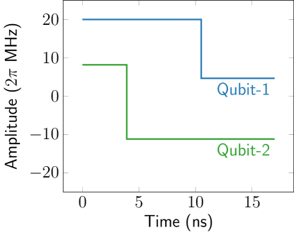
Figure 1: Illustration of a simple square pulse with two time segments.

In this work, we have chosen to impose simple constraints on the form of $\Omega_{n}(t)$ to minimize the number of optimization parameters and simplify experimental implementation. We have considered two examples: i) piecewise-constant pulses, and ii) sum of Gaussian pulses. Because these two examples yield similar results, we present only the square pulse data in the main text, and provide the Gaussian pulse data in the SI. An example of a pair of two-time-segment square pulses for a two transmon system is shown in Figure 1. With a single time segment square pulse, the amplitude is taken as constant throughout the pulse duration. For $n$ time segments, the parameterized square pulse is given by,

$$\Omega_{k}(t)=\begin{cases}c_{1}&0\leq t<t_{1}\\ c_{2}&t_{1}\leq t<t_{2}\\ \vdots\\ c_{n}&t_{n-1}\leq t<T\quad,\end{cases}$$ (9)

where $c_{i}$ are amplitudes of the pulse, $t_{i}$ are the switching times, and $T$ is the total pulse duration. The amplitudes are constrained to $\pm$20 MHz unless otherwise mentioned; this is a typical amplitude for RF control signals in superconducting qubit systems Ku et al. (2017) Each transmon drive term also has a frequency modulation of the form $\mbox{exp}\left(i~{}\nu_{k}t\right),$ with a driving frequency $\nu_{k}$ constrained to $(\omega_{k}-2\pi\text{ GHz})\leq\nu_{k}\leq(\omega_{k}+2\pi\text{ GHz})$, where $\omega_{k},\nu_{k}$ are in units of $2\pi~{}\mbox{GHz}$. Therefore, the pulse parameters that will be optimized include $c_{j}$, $t_{j}$ and $\nu_{k}$. With $N$ transmons and $n$ square pulses on each transmon, we then have $2Nn$ parameters to optimize. The pulse parameter optimizations are performed using l-BFGS-b.

We note that a very recent preprint uses similar quantum control considerations to improve VQE.Choquette et al. (2020) However, in that work, these considerations are used only to define an improved gate-based ansatz, unlike the direct variational pulse shaping described in this work. Our work is also somewhat related to the paper from Chamon and coworkers (Ref. Yang et al., 2017) in which they find that the optimal pulse for preparing the ground state of a Hamiltonian is of a bang-bang form. Although both ctrl-VQE and the work of Ref. Yang et al., 2017 both combine variational quantum algorithms with quantum control, our effort aims to find ground states of non-diagonal Hamiltonians (such as the molecular Hamiltonian in Eq. II.1), preventing the efficient implementation of the time-evolution operator needed for realizing the bang-bang protocol. Because our control Hamiltonian is not determined by our problem Hamiltonian (Eq. II.1), we should not expect such bang-bang protocols to be optimal.

III Computational Details

The numerical results presented in this work were generated with a locally developed program: CtrlQ. Functionalities from QiskitAbraham et al. (2019) and QutipJohansson et al. (2013) were used to check and compare the results presented in this work. Molecular integrals were generated using PySCFSun et al. (2018), and an STO-3G basis set was used throughout. Below, we consider simulations that involve either two-transmon or four-transmon devices depending on the molecule. The parameters $\omega$, $\delta$ and $g$ used in the simulations are explicitly given in Table 1. To demonstrate qualitative insensitivity to the device parameters, we provide some results using a device with a larger detuning in the SI.

Although the simulations presented in the following sections use highly restricted forms of control pulses, our in-house code (CtrlQ) supports various forms of pulses. In fact, we have implemented efficient analytic gradients of the molecular energy with respect to pulse amplitudes (see SI), making it possible to optimize pulses with arbitrary shapes. As mentioned in the previous section, here we focus primarily on simple pulse waveforms with few parameters to simplify experimental implementations.

	Transmon
	1	2	3	4
$\omega$	4.8080	4.8333	4.9400	4.7960
$\delta$	0.3102	0.2916	0.3302	0.2616
	1 $\leftrightarrow{}$2	2 $\leftrightarrow{}$3	3 $\leftrightarrow{}$4	4 $\leftrightarrow{}$1
$g$	0.01831	0.02131	0.01931	0.02031

Table 1: Device parameters appearing in Eq. 3 for a four-transmon system. For the simulations of H₂ and HeH⁺, which only involve two transmons, device parameters corresponding to transmons 1 and 2 were used. All units are in $2\pi~{}\mbox{GHz}$.

IV Results and Discussion

In the following subsections, we explore the ability of ctrl-VQE to reproduce Full Configuration Interaction (FCI) (exact diagonalization) bond dissociation energy curves for two small example diatomic molecules with complementary electron correlation profiles. We then analyze the dependence of the pulse time on the molecule’s electron correlation, followed by a comparison to a representative gate-based circuit. After reporting the new results, we discuss comparisons with related quantum algorithms.

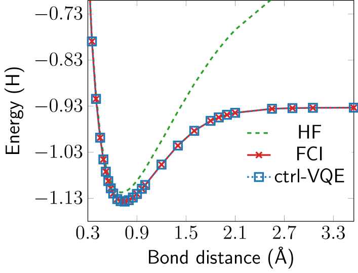
Figure 2: Bond dissociation curve of H₂ molecule. ctrl-VQE energies are computed using square pulses with two time segments.

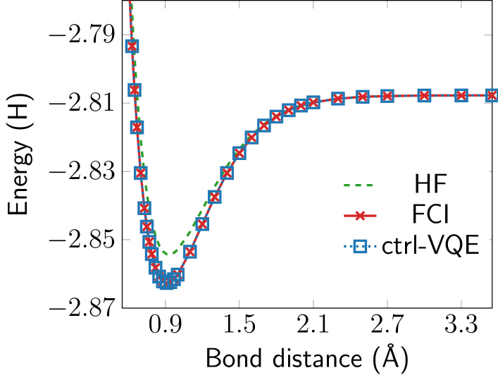
Figure 3: Bond dissociation curve of HeH⁺ molecule. ctrl-VQE energies are computed using square pulses with two time segments.

IV.1 Dissociation of diatomic molecules

Here, we demonstrate the performance of our approach by computing the ground state molecular electronic energy along the bond dissociation of the H₂ molecule and the HeH⁺ molecular ion. Although small, these molecules have been used as benchmarks for quantum algorithms in recent years.Wang et al. (2015); Shen et al. (2017); Kandala et al. (2017); Colless et al. (2018); McCaskey et al. (2019); Gard et al. (2020); Barron et al. (2020a); Xia et al. (2018); Hempel et al. (2018); Sugisaki et al. (2019); Ritter (2019); Sagastizabal et al. (2019); Armaos et al. (2020) These two molecular examples are chosen because they exhibit different behaviors during bond dissocation in terms of their electronic structure. As two-orbital, two-electron problems, these would naturally be modeled on four qubits following the commonly used Jordan-Wigner transformation.Jordan (1928) However, to make the pulse simulations more computationally efficient, we have used the parity mapping instead in which two qubits are diagonal and can be removed from consideration. Details are given in Ref. Bravyi et al. (2017), and we use the implementation for mapping and pruning in Qiskit software.Abraham et al. (2019)

As a prototypical example of a homolytic dissociation,

$$\text{H}_{2} \rightarrow\text{H}^{\bullet}+\text{H}^{\bullet}$$ (10)

Dynamic Correlation $$\rightarrow\text{Static Correlation }$$

as H₂ dissociates, the ground state moves from being dominated by a single Slater determinant to increasingly multiconfigurational, due to the shrinking HOMO-LUMO gap. As a result, the accuracy of a mean-field treatment (e.g., HF) diminishes as the bond length is stretched.

In stark contrast, HeH⁺ becomes easier to model as the bond distance increases. The reason is that, being the strongest acid and, interestingly, the first molecule formed in the universe,Güsten et al. (2019) dissociation is a heterolytic deprotonation,

$$\text{HeH}^{+} \rightarrow\text{He}+\text{H}^{+}$$ (11)

Dynamic Correlation $$\rightarrow\text{No Correlation*}$$

such that both the reactants and the products are both closed shell and well represented by a single Slater determinant. If fact, in a minimal basis set (i.e., the STO-3G basis set used in this paper), the products have exactly zero electron correlation energy because the H⁺ ion has no electrons, while the He atom has no empty virtual orbitals into which electrons can be promoted. As a result, HF becomes exact at dissociation. Of course, in larger basis sets, the He atom would have some dynamic correlation, hence the * in Eq. 11.

The dissociation curves of the H₂ and HeH⁺ molecular systems produced with ctrl-VQE using the simple square pulses are presented in Figs. 2 and 3 respectively. Consistent with the physical descriptions above, the HF state moves quickly away from the FCI ground state with bond dissociation for H₂, while the opposite is true for HeH⁺, where the HF state gradually converges to the exact FCI ground state with increasing bond distance. ctrl-VQE reproduces the FCI bond dissociation curve of H₂ and HeH⁺ with high accuracies. The maximum difference from the FCI energy along the dissociation curve is $.03$ mHa for both H₂ and HeH⁺, and the average error is $.002$ mH in both the cases. More detailed information including the pulse parameters, characteristics, and molecular energies along the dissociation curves are provided in the SI. The resulting states have a good overlap with the exact FCI ground states (99% in all cases). For H₂, it is possible for the overlap to deviate at long bond distances due to degenerate singlet and triplet states. As the bond distance increases, the singlet ground state of H₂ becomes degenerate with the lowest triplet state, making it possible to generate a superposition of a singlet and triplet. It is possible to converge to the exact ground singlet state by supplementing the objective function with a penalty term proportional to the total spin operator (see SI for details).

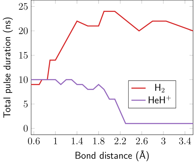
Figure 4: Total pulse duration as a function of bond distance of H₂ and HeH⁺ molecular systems. Square pulses were used to generate the ctrl-VQE molecular energies in Figs. 2 and 3. The shortest pulse duration at each geometry is plotted here.

IV.2 Effect of electron correlation on pulse duration

In any VQE, one is typically interested in finding a useful balance between accuracy (needing deep circuits) and noise (needing shallow circuits). As such, molecular simulations of strongly correlated molecules are intrinsically more difficult as deeper circuits are required, which increases problems from noise and gate errors. An analogous balance is targeted in ctrl-VQE, where one would hope to obtain sufficiently accurate results with as short of a pulse time as possible. Because entanglement cannot be created instantly,Deffner and Campbell (2017) we expect molecules with strong correlation to require longer pulses than simpler molecules.

In order to examine this relationship, in Fig. 4 we plot the duration of the shortest pulses we were able to obtain at each molecular geometry, with H₂ (HeH⁺) shown in red (purple). Referring back to Eqs. 10 and 11, one would expect that as the bond distance is increased, H₂, needing more entanglement, would in turn require increasing pulse durations, whereas pulses for HeH⁺ would get increasingly fast as the bond is stretched. This trend is indeed observed.

The total pulse duration significantly decreases for the dissociation of the HeH⁺ molecular ion, whereas it significantly increases for the H₂ molecule. Note that the initial state and the final target state for HeH⁺ become degenerate with increasing bond distance (above 2.0 Å). Thus, the Hartree Fock state ($\ket{01}$) is a good approximation to the exact FCI ground state, and only a slight modification to the initial state is required to well approximate the ground state. With ctrl-VQE, the total pulse duration at the far bond distances of HeH⁺ are only 1.0 ns. This directly reflects the efficiency of the method presented in this work. In a gate-based compilation method, generally one would still construct an ansatz comprised of costly two-qubit gates, even though the target state is very nearly approximated by the initial state.

The total pulse duration at the dissociation limit for H₂ is significantly longer than near the equilibrium bond distance. Although the HF molecular energy increases monotonically beyond the equilibrium point, the same is not observed for the pulse duration. This is suggestive of the pulse durations reflecting the different dynamics along the bond dissociation of the two molecular systems (see SI for a more detailed analysis).

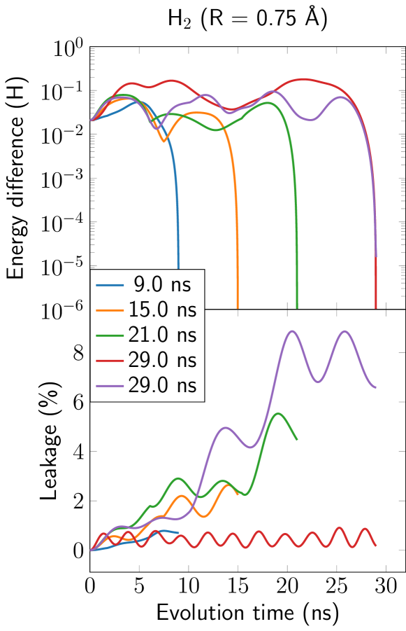
Figure 5: Energy difference between ctrl-VQE and FCI (top) and leakage (bottom) along the time evolution steps with optimal pulses of different durations for H₂ with a bond distance of 0.75 Å. The red and purple lines with $T=29$ ns are distinct solutions to the same optimization. Optimized pulse parameters are provided in the SI.

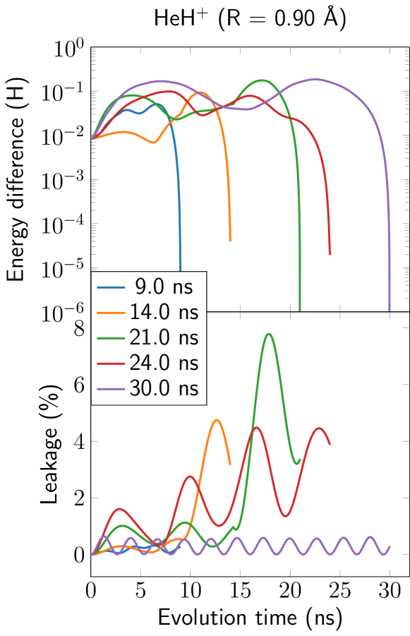
Figure 6: Energy difference between ctrl-VQE and FCI (top) and leakage (bottom) along the time evolution steps with optimal pulses of different durations for HeH⁺ with a bond distance of 0.90 Å. Optimized pulse parameters are provided in the SI.

IV.3 Leakage to higher energy states

In Figs. 5 and 6, we show the energy and leakage as a function of evolution time for various choices of the hyper-parameter, $T$, (the total evolution time). In each of the two figures, the top panel displays the behaviour of the molecular energy as the state evolves from the reference Hartree-Fock state to the converged trial state, and the bottom panel displays the total population outside of the $\ket{0}$ and $\ket{1}$ computational states for each qubit (leakage).

We see that for each value of $T$, the molecular energy of both H₂ and HeH⁺ never decreases toward the exact energy monotonically, but rather increases initially, and then either decreases or oscillates before rapidly converging to the exact energy. While each of the optimized pulses do indeed generate suitable transmon dynamics which accurately produce the molecular ground state at the specified time $T$, the different pulses are not each equally favorable. From the bottom panels of Figs. 5 and 6, we see that some pulses create much more leakage than other pulses. High levels of leakage will likely require a larger number of shots (pulse executions) to get precise determinations of the expectation values, since a higher portion of the shots end up in excited states which are either discarded, or collected for normalizing the results. However, with leakage of only 10%, we anticipate only needing a commensurate increase in the shot count to compensate for post-selection, and so we do not expect this to be a fundamental limitation of the approach. Alternatively, one can use an unnormalized energy in the objective function. This approach naturally constrains the solutions to simultaneously minimize leakage, as any leakage necessarily penalizes the associated pulse. Results using an unnormalized energy in the objective function are comparable to those shown here, and are given in the SI.

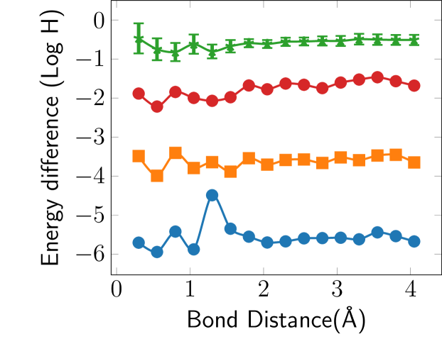
Figure 7: Energy error for the dissociation of H₂. Instead of using the exact, optimized parameters, we use parameters which have added Gaussian noise uncertainty. For each optimal parameter, we randomly sample 100 points each from a Gaussian distribution centered on its optimal setting and with a standard deviation of $\sigma=\{10^{-4},10^{-3},10^{-2},10^{-1}\}$ which correspond to the blue, orange, red and green curves respectively. The resulting energies for these 100 trials are then averaged. Error bars are given for each point but are smaller than some markers.

IV.4 Noise analysis: Imprecise control

All the analysis thus far has assumed perfect control over the driving parameters used to generate approximate ground states of chemical Hamiltonians. However, there are always uncertainties when attempting to implement the optimal driving parameters. In Fig. 7 we simulate the effect of imprecisely implementing these parameters. For each set of optimal drive parameters found by the ctrl-VQE protocol, we produce 100 samples of noisy parameters taken from Gaussian distributions that are centered about the optimal parameter values:

$$\theta_{n}\leftarrow\mathrm{exp}\left(-\frac{(\theta-\theta_{o})^{2}}{2\sigma^{2}}\right),$$ (12)

where $\theta_{n}$ is a noisy version of the optimal parameter $\theta_{o}$. These in turn are used to produce 100 noisy energy samples. We then average these 100 samples and find the resulting energy difference relative to the target ground state energy. With this applied noise model, we can see that even imprecise settings can still be used to achieve accuracies below a $10^{-4}$ energy error. As shown in the red and green curves in Fig. 7, only when the noise becomes higher than $\sigma=0.01$ (where errors reach a magnitude of $10~{}\mbox{MHz}$ or $1~{}\mbox{ns}$) do the energy differences become significant enough to affect the performance of ctrl-VQE. Since these errors are of the same order as the parameters themselves, they do not hinder the realistic implementation of ctrl-VQE. We do not include any explicit noise due to finite decoherence ($T_{1}$) or dephasing ($T_{2}^{*}$) since the pulses we find are many orders of magnitude shorter than the typical time scales for these effects.Koch et al. (2007) To confirm this, we ran simulations using a Lindblad master equation that includes these effects. Our objective function did not change significantly due to our short time scales.

IV.5 Comparison with Circuit Compilation Techniques

Although several ansätze have been proposed to achieve shorter circuits, even the most compact approaches involve too many gates to implement on current hardware for all but the smallest molecules. In order to reduce the time spent during the state-preparation stage, and thus the coherence time demands on the hardware, circuit compilation techniques have been designed to take a given quantum circuit and execute it either with fewer gates or by reoptimizing groups of gates for faster execution.

To execute the gate-based VQE (described in Section II.1) experimentally, the gates in a circuit are compiled to sequences of analog control pulses using a look-up table that maps each elementary gate to the associated predefined analog pulse. The sequence of control pulses corresponding to the elementary gates in the quantum circuit are then simply collected and appropriately scheduled to be executed on the hardware. As such the compilation is essentially instantaneous, making the gate-based compilation technique well suited for VQE algorithms where numerous iterations are performed.

From a compactness perspective however, this gate-based compilation is far from ideal, resulting in total pulse durations which are much longer than what might be obtained with optimized compilation techniques. As is obvious from the one-to-one translation of gates to pulses, the overall circuit structure is typically not considered in gate-based compilations. Thus one may naturally be inclined to seek an optimal pulse sequence for the entire circuit. This has motivated compilation algorithms where control pulses are optimized for the target circuit, using numerical optimal control techniques such as gradient ascent pulse engineering (GRAPE)Khaneja et al. (2005) for partially optimal compilation.Gokhale et al. (2019) However, because the GRAPE algorithm itself is highly non-trivial, the compilation latency for each iteration is of critical concern. Two of the GRAPE-based techniques are briefly described below; see Ref. 61 for a detailed discussion.

The GRAPE compilation technique employs an optimal control routine which compiles to machine-level sequences of analog pulses for a target quantum circuit. This is achieved by manipulating the sets of time-discrete control fields that are executed on the quantum system. The control fields in the optimal routine are updated using gradients (see Ref. 62 for use of analytical gradients) of the cost function with respect to the control fields. GRAPE compilation achieves up to 5-fold speedups compared to standard gate-based compilation. However, such speedup comes with a substantial computational cost. This amounts to long compilation latency, making this approach impractical for VQE algorithms in which multiple iterations of circuit-parameter optimizations are performed. The GRAPE-based compilation also suffers from limitations in the circuit sizes it can handle Lu et al. (2017); Gradl et al. (2006); Cheng et al. (2020).

On the other hand, partial compilation techniques achieve significant pulse speedups by leveraging the fast compilation of standard gate-based techniques together with the pulse speedups of GRAPE-based compilations. Two flavors of such an approach were reported in Ref. 61. Both divide the whole circuit into blocks of subcircuits. In the so-called strict partial compilation, the structure of quantum circuits used in quantum variational algorithms are exploited to only perform GRAPE-based compilation on fixed subcircuits that are independent of the circuit parametrization. The optimal pulses using the GRAPE compilation techniques for the fixed blocks are pre-computed and simply concatenated with the control pulses from the gate-based compilations for the remaining blocks of the circuit. Thus, the compilation speed is comparable to the gate-based compilations in each iteration, but this method also takes advantage of pulse speedups from GRAPE-based compilations. As one may expect, the pulse speedups heavily depend on the circuit depth of the fixed blocks.

In the other flavor, flexible partial compilation, circuits are blocked into subcircuits, each with a single variational parameter, ensuring the subcircuit blocks have low depth. Hyperparameter optimizations are performed for each subcircuit, and they are utilized to find optimal pulses for the circuit blocks. It is noteworthy to mention that in the flexible partial compilation, compilation latency is reduced significantly (around 80x, see Ref. 61) by tuning the hyperparameters of the circuit blocks to speed up the convergence of optimal control in GRAPE. Flexible partial compilations achieve significant pulse speedups as compared to strict partial compilations. However, in spite of the high pulse speedups, the flexible partial compilation technique still diverges from the extremely fast compilation time of the standard gate-based methods. Thus, the algorithm still suffers from compilation latency, albeit to a lesser degree compared to GRAPE-based compilation.

Although both of these GRAPE-based compilation techniques and ctrl-VQE share a direct pulse-shaping step, they fundamentally differ because ctrl-VQE is not a compiler. In contrast to full or partial compiling, we make no reference to a circuit or to implementing any specific unitary. Of course, the control pulses we find do implement some equivalent circuit or unitary (and we analyze these in Sec. IV.6), but we have no need to ever characterize the unitary. In fact, because ctrl-VQE only targets a single state, a large family of unitaries (defined by the behavior in the spaces orthogonal to the initial and final states) exist which minimize our objective function. As such, many possible solutions exist, with no immediate preference given to any one.

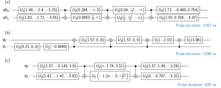
Figure 8: Illustration of circuits constructed using the unitary and state vectors from ctrl-VQE. (a) Circuit corresponding to unitary obtained from a KAK decomposition. (b) An arbitary circuit corresponding to the state vector. (c) Transpiled version of circuit (b).

IV.6 Decompiled control pulses

In the previous sections, the efficiency of ctrl-VQE using optimized control pulses at the device level was demonstrated. The short pulse durations imply that applications to larger molecules might have even more significant speedup since the number of CNOTs in most VQE ansätze increases quickly.

Although ctrl-VQE is performed using no state preparation circuit, the unitary created by the time dynamics of the applied pulse can be decomposed into gates, allowing one to analyze the circuit. This is essentially running a compiler in reverse, or “decompiling” the pulse to yield a state preparation circuit. With this decompiled circuit at hand, we can evaluate the time it would take to execute the optimized pulse as a traditional circuit. By comparing this time to that of the pulse duration, one has a clean benchmark for quantifying the overhead associated with gate-based state preparation. This decompilation can be done in two ways. In the first approach, we simply compute the matrix representation of the evolution operator generated by the optimized ctrl-VQE pulse. For the two-qubit case in focus here, a quantum circuit is then constructed using the KAK decomposition technique. For a detailed description of the technique, we refer the reader to Ref. 66.

In the second approach, an arbitrary circuit corresponding to the state vector from ctrl-VQE is constructed and then transpiled to obtain a shorter circuit depth. In this way we obtained gate durations on IBMQ hardware (mock Johannesburg device available in Qiskit software). The KAK decomposition, arbitrary circuit construction, transpilation and the mock circuit compilations were performed using Qiskit software Abraham et al. (2019). The quantum circuits are illustrated in Figure 8. The corresponding pulse durations are 1202 ns for the circuit obtained using the KAK decomposition and 825 ns for the circuit obtained from transpilation. The state vector used in this study was for the H₂ molecule at 0.75 Å, and the corresponding pulse duration was 9 ns with ctrl-VQE. This clearly demonstrates that state preparation circuits can be much deeper than is necessary.

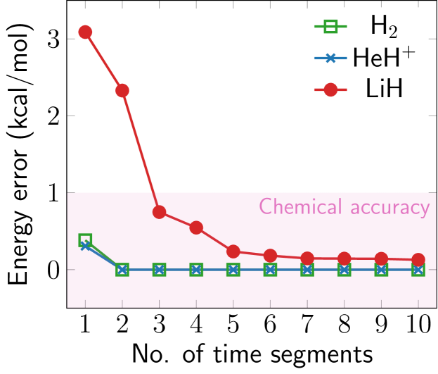
Figure 9: Convergence of pulse parameterization: Energy difference of ctrl-VQE relative to FCI with increasing number of time-segments in the square pulse used.

Method	Energy	Error
Hartree-Fock	-7.8633576	0.0177
ctrl-VQE	-7.8806399	0.0004
FCI	-7.8810157	–
Pulse duration	40 ns
Leakage	0.59 %
Overlap	99.38 %

Table 2: Performance of ctrl-VQE in computing the ground state energy of the LiH molecule (Li-H R = 1.5 Å). The energy error relative to FCI, the leakage to higher energy states, the total pulse duration, and the overlap with the exact FCI state are shown. The data correspond to the pulse with five time segments from Fig. 9.

IV.7 Adaptive update of pulse parameterization

The manner in which a pulse is parameterized (in particular, the number of variational parameters) will significantly impact experimental performance. An over-parameterization of the pulse leads to difficulties in experimental optimization. In response, we seek a means to limit the number of parameters. In this section, we describe a scheme to avoid over-parameterizations and arrive at the minimal number of pulse parameters to achieve a target accuracy.

Unlike in the previous sections where we chose a fixed number of time segments, in this section we propose an adaptive algorithm which slowly grows the number of segments (and thus parameters). We begin with a single time-segment square pulse (constant amplitude throughout the time evolution), the pulse is then iteratively sliced at random intervals such that the number of time segments systematically increases. This adaptive scheme is outlined below:

1. Initialize a parameterized square pulse with $n=1$ time segment and perform the variational pulse optimization.

2. Divide the pulse obtained from the previous step at a randomly choosen time. The square pulse now has $n=2$ time segments.

3. Perform pulse optimization using the pulse shape from the previous step as an initial guess.

4. Divide the largest time segment in the square pulse obtained from the previous step into two at a randomly chosen time. This increases the number of segments from $n$ to $n+1$.

5. Perform pulse optimization using the pulse shape from the previous step as an initial guess.

6. Repeat Steps 4 and 5 until the energy obtained is sufficiently converged.

Note that drive frequencies for the pulses are also optimized in the above procedure. Irrespective of the pulse shape used, only a single drive frequency is used for each qubit. The switching times for the square pulses with more than one time segment are not optimized and remain fixed in Steps 3 and 5. For $N$ transmons with $n$ pulse time segments each, the total number of parameters to optimize is $N(n+1)$. In the following simulations, we constrain the amplitudes and drive frequencies within the ranges $\pm 40$ MHz and $\omega_{k}\pm 3\pi$ GHz, respectively.

Following the above strategy of adaptively increasing the number of time segments in the square pulses, we obtained optimal pulses for H₂, HeH⁺ and LiH with total pulse durations of 9, 9 and 40 ns respectively. Fig. 9 plots the energy difference relative to FCI with increasing number of time segments in the optimal pulse. For H₂ and HeH⁺, chemical accuracy is obtained with a single-time-segment square pulse on each qubit, while for LiH, three time segments are required to achieve chemical accuracy. The molecular energy converges for square pulses with two time segments for H₂ and HeH⁺ and with five time segments for LiH molecules. The error in ground state energy of LiH molecule (Li-H R=1.5 Å) computed with ctrl-VQE along with pulse duration, leakage and overlap with the exact FCI state is tabulated in Table 2. To illustrate the sequential pulse refinement from iteration to iteration, the square pulse shapes at each adaptive step for LiH are shown in Fig. 10.

In the case of LiH, we see that the accuracy is not of the same order as in the other two diatomic molecules. To further examine this, we perform over 100 pulse optimizations on the square pulse with 10 time segments obtained from the adaptive strategy by retaining only the switching times and starting with random amplitudes and drive frequencies. We use a large number of initial guesses to reduce the likelihood of getting trapped in a local minimum. We find that the highest accuracy is achieved when we use the pulse obtained from the adaptive strategy above. This suggests that we are nearing the accuracy limit of LiH using a 40 ns pulse.

While the above adaptive strategy aims at practical experimental implementation, the cost of classical simulation remains the same irrespective of the number of time-segments when analytical gradients for the pulse amplitudes are used. The cost of evaluating an analytical gradient is only about 2.5 times the cost of an energy evaluation. Here, the analytical gradient is obtained at each trotter step of time evolution and adapted for the pulse shaped considered. Details along with the derivation are provided in the SI.

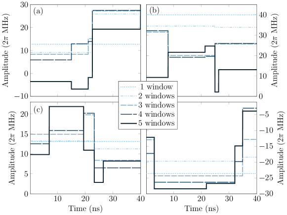
Figure 10: Adaptive increase of pulse windows for LiH molecule: Square pulse shapes obtained at each adaptive step, starting from one time window and adaptively dividing the time window up to five-segments. The accuracy increases with each division of the pulse. Pulse shapes are shown for the pulses on (a) qubit 1, (b) qubit 2, (c) qubit 3, (d) qubit 4.

IV.8 Comparison to gate-based ansätze

Now we directly compare the results of our pulse-based technique with gate-based variational ansätze. We use calibration data from an IBMQ device (mock Johannesburg device available in Qiskit software) to compute the duration of the circuits used to prepare trial wavefunctions. We consider the RY and UCCSD ansätze, which are capable of producing the exact ground state.

For both H₂ and HeH⁺, the RY ansatz requires 1 CNOT, and the UCCSD requires 2 CNOTs. The RY ansatz has 4 parameters, and the UCCSD ansatz has 3 parameters. The total pulse time of the RY ansatz is 519 ns, and the UCCSD ansatz is 825 ns. For the LiH molecule, the RY and UCCSD ansätz require 9 and 245 CNOTs respectively. The RY ansatz has 16 parameters whereas the UCCSD ansatz has 8 parameters. The total pulse duration of the RY ansatz is 3485 ns, and that of the UCCSD ansatz is 82169 ns for LiH. In each case, the time to execute the circuit is significantly longer than the time required to apply the pulses using ctrl-VQE, which is 9 ns for H₂ and HeH⁺, and 40 ns for LiH. The $T_{1}$ and $T_{2}$ times of the IBMQ device used range from 45150 to 115217 ns (average 71262 ns) and from 48173 to 107025 ns (average 74490 ns) respectively. This means that the pulse duration for LiH using the UCCSD ansatz is already reaching the limit set by decoherence times of the device, while the pulse duration obtained with ctrl-VQE is well within the decoherence time.

We note here that this comparison needs to be approached with a bit of caution, as our simulated device has slightly different parameters than the IBM-Q devices used for the circuit timings. However, we do not expect that our results would change significantly if we had access to the full set of exact parameters of the device (including anharmonicities, bus frequencies, and couplings), because previous works using the present device parameter regimeEconomou and Barnes (2015); Barron et al. (2020b) have demonstrated universal gate sets with single and two-qubit operations commensurate with those of the IBM-Q devices. As such, we expect the ctrl-VQE pulse times reported in this study to be close to what one would get by directly running the calculations on IBM-Q devices.

V Summary and Future Outlook

We have presented a new variational quantum algorithm which is fundamentally different from the existing quantum algorithms for molecular simulation. The quantum circuit used for state preparation in standard variational algorithms is entirely replaced by a hardware-level control routine with optimized pulse shapes to directly drive the qubit system. The efficacy of the presented method is numerically demonstrated by modeling the bond dissociation of two diatomic molecules, H₂ and HeH⁺. The maximum error from the exact FCI energy is well within chemical accuracy (0.02 kcal/mol) for both molecular systems throughout the bond dissociation. ctrl-VQE captures the important electron correlation effects involved in the bond dissociation of the two molecular systems, as reflected in the pulse durations along the bond dissociation. To demonstrate the application of ctrl-VQE to a larger molecular system, we have also computed the energy of the LiH molecule at a single bond distance. An adaptive scheme which slowly increases the variational flexibility of the pulse parameterization was used to determine the minimal number of pulse parameters required to acheive a target accuracy, ultimately simplifying experimental implementation and avoiding over-parameterization. The results demonstrate that pulse shapes with relatively modest numbers of parameters achieve convergence in the energy even as the problem size increased. The approach yields significant state-preparation speedups for VQE as compared to standard gate-based ansätze. The short pulse durations minimize losses due to decoherence and dephasing, which is a step toward enabling more accurate VQE simulations on larger, strongly correlated systems. ctrl-VQE can be viewed as a lowest-level quantum variational algorithm.

Because ctrl-VQE operates directly on the hardware, classical simulations of the algorithm are even more computationally expensive than typical VQE emulations, as one needs to not only solve the time-dependent Schrödinger equation, but also optimize the driving Hamiltonian. As such, the systems we have been able to study so far are very small. In future work, we will develop an improved implementation to study the behavior of larger systems and with more sophisticated constraints on the pulse shape ($\Omega_{n}(t)$). Improved software will also make it possible to numerically study the impact that device controllability limitationsBall et al. (2020) have on the amount or type of electron correlation able to be described.

Competing Interest Statement

The Authors declare no Competing Financial or Non-Financial Interests.

Data Availability

The data for the numerical simulations is available upon reasonable request.

Code Availability

The code for the numerical simulations is available at https://github.com/mayhallgroup/ctrlq.

Author Contributions

N.J.M., S.E.E, E.B., and D.P.P. conceived the project. O.R.M. wrote the python/C++ code and helped design the adaptive pulse parameterization algorithm. B.T.G. wrote mathematica code. B.T.G. and O.R.M performed numerical experiments. All authors contributed to the conceptual analysis of the results and to ideas that refined the algorithm. All authors wrote the paper.

VI Acknowledgements

N.J.M., S.E.E., E.B., and D.P.P are grateful for financial support provided by the U.S. Department of Energy (Award No. DE-SC0019199). S.E.E acknowledges support provided by the U.S. Department of Energy (Award No. DE-SC0019318). This work was done in part while N.J.M. was visiting the Simons Institute for the Theory of Computing. The authors thanks the Advanced Research Computing at Virginia Tech for the computational infrastructure.

References

- White (1992) S. R. White, Physical Review Letters 69, 2863 (1992).
- Chan and Head-Gordon (2002) G. K.-L. Chan and M. Head-Gordon, J. Chem. Phys. 116, 4462 (2002), ISSN 0021-9606.
- Schollwöck (2011) U. Schollwöck, Annals of Physics 326, 96 (2011).
- Huron et al. (1973) B. Huron, J. P. Malrieu, and P. Rancurel, J. Chem. Phys. 58, 5745 (1973), ISSN 00219606, URL http://link.aip.org/link/?JCPSA6/58/5745/1.
- Bender and Davidson (1969) C. F. Bender and E. R. Davidson, Phys. Rev. 183, 23 (1969), URL https://link.aps.org/doi/10.1103/PhysRev.183.23.
- Buenker (1968) R. J. Buenker, J. Chem. Phys. 49, 5381 (1968), ISSN 00219606.
- Evangelisti et al. (1983) S. Evangelisti, J.-P. Daudey, and J.-P. Malrieu, Chemical Physics 75, 91 (1983), ISSN 0301-0104.
- Tubman et al. (2016) N. M. Tubman, J. Lee, T. Y. Takeshita, M. Head-Gordon, and K. B. Whaley, J. Chem. Phys. 145, 044112 (2016), ISSN 0021-9606.
- Schriber and Evangelista (2016) J. B. Schriber and F. A. Evangelista, The Journal of Chemical Physics 144, 161106 (2016).
- Holmes et al. (2016) A. A. Holmes, N. M. Tubman, and C. J. Umrigar, Journal of Chemical Theory and Computation 12, 3674 (2016).
- Levine et al. (2020) D. S. Levine, D. Hait, N. M. Tubman, S. Lehtola, K. B. Whaley, and M. Head-Gordon, J. Chem. Theory Comput. 16, 2340 (2020), ISSN 1549-9618.
- Caffarel et al. (2016) M. Caffarel, T. Applencourt, E. Giner, and A. Scemama, in Recent Progress in Quantum Monte Carlo (American Chemical Society, 2016), vol. 1234 of ACS Symposium Series, chap. 2, pp. 15–46, ISBN 978-0-8412-3179-5.
- Abraham and Mayhall (2020) V. Abraham and N. J. Mayhall, J. Chem. Theory Comput. 16, 6098 (2020), ISSN 1549-9618.
- Peruzzo et al. (2014) A. Peruzzo, J. McClean, P. Shadbolt, M.-H. Yung, X.-Q. Zhou, P. J. Love, A. Aspuru-Guzik, and J. L. O’Brien, Nature communications 5, 4213 (2014), ISSN 2041-1723 (Electronic) 2041-1723 (Linking).
- Preskill (2018) J. Preskill, Quantum 2, 79 (2018), ISSN 2521-327X.
- Sharma et al. (2020) K. Sharma, S. Khatri, M. Cerezo, and P. J. Coles, New Journal of Physics 22, 043006 (2020), URL https://doi.org/10.1088%2F1367-2630%2Fab784c.
- Kandala et al. (2017) A. Kandala, A. Mezzacapo, K. Temme, M. Takita, M. Brink, J. M. Chow, and J. M. Gambetta, Nature 549, 242 (2017), URL https://doi.org/10.1038/nature23879.
- Huggins et al. (2019a) W. J. Huggins, J. Lee, U. Baek, B. O’Gorman, and K. B. Whaley, arXiv:1909.09114 [physics, physics:quant-ph] (2019a), eprint 1909.09114.
- Lee et al. (2019) J. Lee, W. J. Huggins, M. Head-Gordon, and K. B. Whaley, J. Chem. Theory Comput. 15, 311 (2019), ISSN 1549-9618.
- Gard et al. (2020) B. T. Gard, L. Zhu, G. S. Barron, N. J. Mayhall, S. E. Economou, and E. Barnes, npj Quantum Information 6, 1 (2020), ISSN 2056-6387.
- Barron et al. (2020a) G. S. Barron, B. T. Gard, O. J. Altman, N. J. Mayhall, E. Barnes, and S. E. Economou, arXiv:2003.00171 [quant-ph] (2020a).
- Ryabinkin et al. (2018) I. G. Ryabinkin, T.-C. Yen, S. N. Genin, and A. F. Izmaylov (2018).
- Grimsley et al. (2019) H. R. Grimsley, S. E. Economou, E. Barnes, and N. J. Mayhall, Nat. Commun. 10, 3007 (2019), ISSN 2041-1723.
- Tang et al. (2020) H. L. Tang, V. O. Shkolnikov, G. S. Barron, H. R. Grimsley, N. J. Mayhall, E. Barnes, and S. E. Economou, arXiv:1911.10205 [quant-ph] (2020), eprint 1911.10205.
- Ryabinkin et al. (2020) I. G. Ryabinkin, R. A. Lang, S. N. Genin, and A. F. Izmaylov, J. Chem. Theory Comput. 16, 1055 (2020), ISSN 1549-9618.
- Jordan (1928) W. Jordan, P., Z. Physik 47, 631 (1928), URL https://doi.org/10.1007/BF01331938.
- Bravyi and Kitaev (2002) S. B. Bravyi and A. Y. Kitaev, Ann. Phys. 298, 210 (2002), URL https://doi.org/10.1006/aphy.2002.6254.
- Seeley et al. (2012) J. T. Seeley, M. J. Richard, and P. J. Love, The Journal of Chemical Physics 137, 224109 (2012), eprint https://doi.org/10.1063/1.4768229, URL https://doi.org/10.1063/1.4768229.
- Bartlett and Musiał (2007) R. J. Bartlett and M. Musiał, Rev. Mod. Phys. 79, 291 (2007), URL https://link.aps.org/doi/10.1103/RevModPhys.79.291.
- Yung et al. (2014) M.-H. Yung, J. Casanova, A. Mezzacapo, J. McClean, L. Lamata, and E. Aspuru-Guzik, A.and Solano, Scientific Reports 4, 3589 (2014).
- Ostaszewski et al. (2019) M. Ostaszewski, E. Grant, and M. Benedetti, arXiv:1905.09692 [quant-ph] (2019), eprint 1905.09692.
- Chivilikhin et al. (2020) D. Chivilikhin, A. Samarin, V. Ulyantsev, I. Iorsh, A. R. Oganov, and O. Kyriienko, arXiv:2007.04424 [cond-mat, physics:quant-ph] (2020), eprint 2007.04424.
- Matsuzawa and Kurashige (2020) Y. Matsuzawa and Y. Kurashige, Journal of Chemical Theory and Computation 16, 944 (2020).
- Huggins et al. (2019b) W. J. Huggins, J. Lee, U. Baek, B. O’Gorman, and K. B. Whaley, arXiv:1909.09114 [physics, physics:quant-ph] (2019b), eprint 1909.09114.
- Lee et al. (2018) J. Lee, W. J. Huggins, M. Head-Gordon, and K. B. Whaley (2018).
- Babbush et al. (2018) R. Babbush, N. Wiebe, J. McClean, J. McClain, H. Neven, and G. K.-L. Chan, Physical Review X 8, 011044 (2018).
- Verteletskyi et al. (2020) V. Verteletskyi, T.-C. Yen, and A. F. Izmaylov, The Journal of Chemical Physics 152, 124114 (2020), eprint https://doi.org/10.1063/1.5141458, URL https://doi.org/10.1063/1.5141458.
- Huggins et al. (2019c) W. J. Huggins, J. McClean, N. Rubin, Z. Jiang, N. Wiebe, K. B. Whaley, and R. Babbush, arXiv:1907.13117 [physics, physics:quant-ph] (2019c), eprint 1907.13117.
- Zhao et al. (2020) A. Zhao, A. Tranter, W. M. Kirby, S. F. Ung, A. Miyake, and P. J. Love, Phys. Rev. A 101, 062322 (2020), URL https://link.aps.org/doi/10.1103/PhysRevA.101.062322.
- Koch et al. (2007) J. Koch, T. M. Yu, J. Gambetta, A. A. Houck, D. I. Schuster, J. Majer, A. Blais, M. H. Devoret, S. M. Girvin, and R. J. Schoelkopf, Phys. Rev. A 76, 042319 (2007).
- Deffner and Campbell (2017) S. Deffner and S. Campbell, J. Phys. A: Math. Theor. 50, 453001 (2017), URL https://doi.org/10.1088/1751-8121/aa86c6.
- Ku et al. (2017) H. S. Ku, J. L. Long, X. Wu, M. Bal, R. E. Lake, E. Barnes, S. E. Economou, and D. P. Pappas, Phys. Rev. A 96, 042339 (2017), URL https://link.aps.org/doi/10.1103/PhysRevA.96.042339.
- Choquette et al. (2020) A. Choquette, A. Di Paolo, P. K. Barkoutsos, D. Sénéchal, I. Tavernelli, and A. Blais, arXiv:2008.01098 [quant-ph] (2020), eprint 2008.01098.
- Yang et al. (2017) Z.-C. Yang, A. Rahmani, A. Shabani, H. Neven, and C. Chamon, Phys. Rev. X 7, 021027 (2017).
- Abraham et al. (2019) H. Abraham, AduOffei, I. Y. Akhalwaya, G. Aleksandrowicz, T. Alexander, E. Arbel, A. Asfaw, C. Azaustre, AzizNgoueya, P. Barkoutsos, et al., Qiskit: An open-source framework for quantum computing (2019).
- Johansson et al. (2013) J. Johansson, P. Nation, and F. Nori, Computer Physics Communications 184, 1234 (2013), ISSN 0010-4655, URL http://www.sciencedirect.com/science/article/pii/S0010465512003955.
- Sun et al. (2018) Q. Sun, T. C. Berkelbach, N. S. Blunt, G. H. Booth, S. Guo, Z. Li, J. Liu, J. D. McClain, E. R. Sayfutyarova, S. Sharma, et al., WIREs Computational Molecular Science 8, e1340 (2018), eprint https://onlinelibrary.wiley.com/doi/pdf/10.1002/wcms.1340, URL https://onlinelibrary.wiley.com/doi/abs/10.1002/wcms.1340.
- Wang et al. (2015) Y. Wang, F. Dolde, J. Biamonte, R. Babbush, V. Bergholm, S. Yang, I. Jakobi, P. Neumann, A. Aspuru-Guzik, J. D. Whitfield, et al., ACS Nano 9, 7769 (2015), ISSN 1936-0851.
- Shen et al. (2017) Y. Shen, X. Zhang, S. Zhang, J.-N. Zhang, M.-H. Yung, and K. Kim, Phys. Rev. A 95, 020501 (2017), URL https://link.aps.org/doi/10.1103/PhysRevA.95.020501.
- Colless et al. (2018) J. I. Colless, V. V. Ramasesh, D. Dahlen, M. S. Blok, M. E. Kimchi-Schwartz, J. R. McClean, J. Carter, W. A. de Jong, and I. Siddiqi, Phys. Rev. X 8, 011021 (2018), URL https://link.aps.org/doi/10.1103/PhysRevX.8.011021.
- McCaskey et al. (2019) A. J. McCaskey, Z. P. Parks, J. Jakowski, S. V. Moore, T. D. Morris, T. S. Humble, and R. C. Pooser, npj Quantum Information 5, 1 (2019), ISSN 2056-6387.
- Xia et al. (2018) R. Xia, T. Bian, and S. Kais, The Journal of Physical Chemistry B 122, 3384 (2018), pMID: 29099600, eprint https://doi.org/10.1021/acs.jpcb.7b10371, URL https://doi.org/10.1021/acs.jpcb.7b10371.
- Hempel et al. (2018) C. Hempel, C. Maier, J. Romero, J. McClean, T. Monz, H. Shen, P. Jurcevic, B. P. Lanyon, P. Love, R. Babbush, et al., Phys. Rev. X 8, 031022 (2018), URL https://link.aps.org/doi/10.1103/PhysRevX.8.031022.
- Sugisaki et al. (2019) K. Sugisaki, S. Nakazawa, K. Toyota, K. Sato, D. Shiomi, and T. Takui, ACS Central Science 5, 167 (2019), eprint https://doi.org/10.1021/acscentsci.8b00788, URL https://doi.org/10.1021/acscentsci.8b00788.
- Ritter (2019) M. B. Ritter, Journal of Physics: Conference Series 1290, 012003 (2019), URL https://doi.org/10.1088%2F1742-6596%2F1290%2F1%2F012003.
- Sagastizabal et al. (2019) R. Sagastizabal, X. Bonet-Monroig, M. Singh, M. A. Rol, C. C. Bultink, X. Fu, C. H. Price, V. P. Ostroukh, N. Muthusubramanian, A. Bruno, et al., Phys. Rev. A 100, 010302 (2019), URL https://link.aps.org/doi/10.1103/PhysRevA.100.010302.
- Armaos et al. (2020) V. Armaos, D. A. Badounas, P. Deligiannis, and K. Lianos, Applied Physics A 126, 625 (2020).
- Bravyi et al. (2017) S. Bravyi, J. M. Gambetta, A. Mezzacapo, and K. Temme, arXiv:1701.08213 [quant-ph] (2017).
- Güsten et al. (2019) R. Güsten, H. Wiesemeyer, D. Neufeld, K. M. Menten, U. U. Graf, K. Jacobs, B. Klein, O. Ricken, C. Risacher, and J. Stutzki, Nature 568, 357 (2019), ISSN 1476-4687.
- Khaneja et al. (2005) N. Khaneja, T. Reiss, C. Kehlet, T. Schulte-Herbrüggen, and S. J. Glaser, Journal of Magnetic Resonance 172, 296 (2005), ISSN 1090-7807, URL http://www.sciencedirect.com/science/article/pii/S1090780704003696.
- Gokhale et al. (2019) P. Gokhale, Y. Ding, T. Propson, C. Winkler, N. Leung, Y. Shi, D. I. Schuster, H. Hoffmann, and F. T. Chong, Proceedings of the 52nd Annual IEEE/ACM International Symposium on Microarchitecture (2019), URL http://dx.doi.org/10.1145/3352460.3358313.
- Boutin et al. (2017) S. Boutin, C. K. Andersen, J. Venkatraman, A. J. Ferris, and A. Blais, Phys. Rev. A 96, 042315 (2017), URL https://link.aps.org/doi/10.1103/PhysRevA.96.042315.
- Lu et al. (2017) D. Lu, K. Li, J. Li, H. Katiyar, A. Park, F. Jihyun, X. Guanru, L. Tao, L. Hang, B. Guilu, et al., npj Quantum Information 3, 45 (2017).
- Gradl et al. (2006) T. Gradl, A. Spörl, T. Huckle, S. J. Glaser, and T. Schulte-Herbrüggen, in Euro-Par 2006 Parallel Processing, edited by W. E. Nagel, W. V. Walter, and W. Lehner (Springer Berlin Heidelberg, Berlin, Heidelberg, 2006), pp. 751–762, ISBN 978-3-540-37784-9.
- Cheng et al. (2020) J. Cheng, H. Deng, and X. Qia, in 2020 ACM/IEEE 47th Annual International Symposium on Computer Architecture (ISCA) (2020), pp. 543–555.
- Williams (2010) C. P. Williams, Explorations in Quantum Computing (Springer, 2010).
- Economou and Barnes (2015) S. E. Economou and E. Barnes, Phys. Rev. B 91, 161405 (2015), URL https://link.aps.org/doi/10.1103/PhysRevB.91.161405.
- Barron et al. (2020b) G. S. Barron, F. A. Calderon-Vargas, J. Long, D. P. Pappas, and S. E. Economou, Phys. Rev. B 101, 054508 (2020b), URL https://link.aps.org/doi/10.1103/PhysRevB.101.054508.
- Ball et al. (2020) H. Ball, M. J. Biercuk, A. Carvalho, J. Chen, M. Hush, L. A. De Castro, L. Li, P. J. Liebermann, H. J. Slatyer, C. Edmunds, et al., arXiv:2001.04060 [quant-ph] (2020), eprint 2001.04060.