Interfaces in spectral asymptotics and nodal sets

Abstract.

This is a survey of results obtained jointly with Boris Hanin and Peng Zhou on interfaces in spectral asymptotics, both for Schrödinger operators on $L^{2}(\mathbb{R}^{d})$ and for Toeplitz Hamiltonians acting on holomorphic sections of ample line bundles $L\to M$ over Kähler manifolds $(M,\omega)$. By an interface is meant a hypersurface, either in physical space $\mathbb{R}^{d}$ or in phase space, separating an allowed region where spectral asymptotics are standard and a forbidden region where they are non-standard. The main question is to give the detailed transition between the two types of asymptotics across the hypersurface (i.e. interface). In the real Schrödinger setting, the asymptotics are of Airy type; in the Kähler setting they are of Erf (Gaussian error function) type.

A principal purpose of this survey is to compare the results in the two settings. Each is apparently universal in its setting. This is now established for Toeplitz operators, but in the Schrödinger setting it is only established for the simplest model operator, the isotropic harmonic oscillator. It is explained that the latter result is most comparable to the behavior of the canonical degree operator on the Bargmann-Fock space of a line bundle, a new construction introduced in these notes.

1. Introduction

This is a mainly expository article on interfaces in spectral asymptotics. Interfaces are studied in many fields of mathematics and physics but seem to be a novel area of spectral asymptotics. Spectral asymptotics refers to the behavior of spectral projections and nodal sets for a quantum Hamiltonian $\hat{H}_{\hbar}$, which might be a Schrödinger operator on $L^{2}(\mathbb{R}^{d})$ or on a Riemannian manifold $(M,g)$, with or without boundary, or a Toeplitz Hamiltonian acting on holomorphic sections $H^{0}(M,L^{k})$ of line bundles over a Kähler manifold. Interface asymptotics refers to the change in behavior of the spectral projections or nodal sets as a hypersurface is crossed, either in physical space (configuration space) or in phase space. Interfaces exist in diverse settings and indeed the purpose of this article is to compare interface behavior in different settings and to consider possible future settings that have yet to be explored.

What is meant by an ‘interface’ in the sense of this article? The general idea is that there is a hypersurface in the phase space separating two regions in which the asymptotic behavior of a spectral projections kernel has different types of behavior: In the first, that we will term the ‘allowed’ region, the asymptotics are constant and, after normalization, equal $1$, so that one has a plateau over the region; in the second ‘forbidden’ region the asymptotics are rapidly decaying, so that one has a rather flat $0$ region. The interface is the shape of the graph of the spectral kernel connecting $1$ and $0$ in a thin region separating the allowed and forbidden region. One expects that when scaled properly, the limit shape is universal. More precisely, universality holds in each type of model (e.g. Schrödinger or Kähler ) but is model-dependent: one expects ‘Airy interfaces’ in the Schrödinger setting and Erf interfaces in the Kähler setting. The separation into different regions for the spectral projections kernel often coincides with the separation of other spectral behavior, such as nodal sets of the eigenfunctions.

The terminology (classically) ‘allowed’ and (classically) ‘forbidden’ is standard in quantum mechanics for regions inside, resp. outside, of an energy surface in phase space, or more commonly, the projection of these regions to configuration space. This will indeed be the meaning of ‘interface’ for most of this article. We will describe results of B. Hanin, P. Zhou and the author [HZZ15, HZZ16] on the different behavior of nodal sets of Schrödinger eigenfunctions in allowed resp. forbidden regions for the simplest Schrödinger Hamiltonian $\hat{H}_{\hbar}$, namely the isotropic Harmonic oscillator on $\mathbb{R}^{d}$. We then consider phase space interfaces of Wigner distributions for the same model, following [HZ19, HZ19b]. We then turn to phase space interfaces in the Kähler (complex holomorphic) setting, and discuss results of Pokorny-Singer [PS], Ross-Singer [RS], P. Zhou and the author [ZZ16, ZZ17] on interfaces for partial Bergman kernel asymptotics. In Section 8 we explain that the exact analogue of the results on Wigner distributions for the isotropic harmonic oscillator in the complex setting is a series of results on interfaces for disc bundles in the Bargmann-Fock space of a line bundle. This Bargmann-Fock space and the interface results constitute the new results of the article.

Roughly speaking, interfaces in spectral asymptotics involve two types of localization: (i) spectral, i.e. quantum, localization where the eigenvalues are constrained to lie in an interval $I$, (ii) classical, i.e. phase space, localization where a phase space point is constrained to lie in an open set $U$ of phase space. It has long been understood that spectral localization $E_{j}(\hbar)\in I$ implies phase space localization in the sense that quantum objects decay in the complement of the allowed region $H^{-1}(I)$. But the study of interfaces is devoted to the precise behavior of quantum objects as one crosses the interface between allowed and forbidden regions, and more generally, considers all possible combinations of spectral localization $E_{j}(\hbar)\in I$ and phase space localization $\zeta\in U$, where $U$ may have any position relative to $H^{-1}(I)$.

Often, the interface corresponds to a sharp cutoff in a spectral parameter and signals something discontinuous. In fact, the earliest studies of interface asymptotics are classical analysis studies of Bernstein polynomials of discontinuous functions with jump discontinuities [Ch, L, Lev, Mir, O]. These studies were intended to be analogues of Gibbs phenomena for Fourier series of discontinuous functions, which have been generalized to wave equations on Riemannian manifolds in [PT97].

In this article we review the following results on interface asymptotics:

• Interface behavior for spectral projections and for nodal sets of random eigenfunctions of energy $E_{N}(\hbar)=\hbar(N+\frac{d}{2})=E$ of the isotropic harmonic oscillator on $\mathbb{R}^{d}$ across the caustic set in physical space, where the potential $V(x)=|x|^{2}/2=E$.

• Interface behavior for Wigner distributions of the same eigenspace projections, and more generally for various types of Wigner-Weyl sums across an energy surface in phase space;

• Interface behavior for the holomorphic analogues of such Wigner distributions, namely for partial Bergman kernels for general Berezin-Toeplitz Hamiltonians on general Kähler phase spaces.

• Interface results for partial Bergman kernels corresponding to the canonical $S^{1}$ action on the total space $L^{*}$ of the dual line bundle of an ample line bundle $L\to M$ over a Kähler manifold.

In the case of Schrödinger operators, the results are only proved in the special case of the isotropic harmonic oscillator. It is plausible that some of the results should be universal among Schrödinger operators, but at the present time the generalizations have not been formulated or proved. See Section 9.1 for further problems. Among other gaps in the theory, Wigner distributions per se are only defined when the Riemannian manifold is $\mathbb{R}^{d}$ and are closely connected to the representation theory of the Heisenberg and metaplectic groups. Wigner distributions of eigenfunctions are special types of “microlocal lifts” of eigenfunctions; there is no generally accepted canonical microlocal lift on a general Riemannian manifold. Despite the restrictive setting, Wigner distributions are important in mathematical physics, in particular in quantum optics. The results in the complex holomorphic (Kähler ) setting are much more complete, due to the fact that the theory of Bergman kernels is technically simpler and more complete than the corresponding theory of Wigner distributions for Schrödinger operators. The results are proved for any Toeplitz Hamiltonian on any projective Kähler manifold. In fact, the exact analogue of the Wigner result is proved in Section 8, where a new construction is introduced in this article: the Bargmann-Fock space of a holomorphic line bundle. It is a Gaussian space of holomorphic functions on the total space $L^{*}$ of the dual of a holomorphic Hermitian line bundle $L\to M$ over a Kähler manifold. This total space carries a natural $S^{1}$ action and this $S^{1}$ action plays the role of the propagator of the isotropic Harmonic Oscillator. Thus, the interfaces are the boundaries of the co-disc bundles $D^{*}_{E}\subset L^{*}$ of different energy levels (i.e. radii). The interface results in Section 8 are a ‘new result’ of this article, but the proofs are similar to, and simpler than, those in [ZZ17, ZZ18] .

This survey is organized as follows:

1. In Section 2, we review the basic linear models: the Harmonic oscillator in the Schrödinger representation on $L^{2}(\mathbb{R}^{d})$ and in the Bargmann-Fock (holomorphic) representation on entire holomorphic functions on $\mathbb{C}^{d}$. We also present a list of analogies between the real Schrödinger setting and the complex holomorphic quantization. Section 3 is devoted to the Bergman kernel on Bargmann-Fock space, and the Bargmann-Fock representations of the Heisenberg and Symplectic groups on Bargmann-Fock space.

2. In Section 4, we review the interface results in physical space for spectral projections for the isotropic Harmonic Oscillator. These imply interface results for nodal sets of random eigenfunctions in a fixed eigenspace.

3. In Section 5, we change the setting to phase space $T^{*}\mathbb{R}^{d}$ and review the interface results in physical space for Wigner distributions of spectral projections for the isotropic Harmonic Oscillator.

4. In Section 6, we switch to the complex holomorphic setting and review interface results for partial Bergman kernels on general compact Kähler manifolds.

5. In Section 7 we specialize to the isotropic harmonic oscillator on the standard Bargmann-Fock space and describe its interfaces;

6. In Section 8 we introduce a new model: the Bargmann-Fock space of a holomorphic line bundle. We then consider interfaces with respect to a natural $S^{1}$ action on this space, generalalizing the previous result on the Bargmann-Fock isotropic Harmonic oscillator.

7. In Section 9.1 we list some further problems on interfaces.

8. In Section 10 we give some background to the holomorphic setting.

1.1. Results surveyed in this article

The articles surveyed in this article are the following:

2. The basic linear models

As mentioned above, our aim in this survey is not only to describe interface results in various settings but to compare the results in the real Schrödinger setting and the complex holomorphic Bargmann-Fock or Berezin-Toeplitz setting. The real setting is self-explanatory to mathematical physicists but the complex holomorphic setting is probably less familiar. In this section, we give some background on the basic linear models (isotropic Harmonic Oscillator in both settings) to make the relations between the real and complex settings more familiar. We then give a list of analogies between the two settings. In addition, we present a list of open problems on interfaces to amplify the scope of spectral interface problems. It would be laborious to present all of the background for the geometric setting before getting to the main results and phenomena, so we have put that background into an Appendix Section 10.

A preliminary remark: Since the early days of quantum mechanics, it was understood that there are many equivalent representations (or ‘pictures’) of quantum mechanics. In the case of $\mathbb{R}^{d}$ they correspond to different but unitarily equivalent representations of the Heisenberg and metaplectic groups (see [F] for background). The most common are the Schrödinger representation on $L^{2}(\mathbb{R}^{d})$ and the Bargmann-Fock representation on $H^{2}(\mathbb{C}^{d},e^{-|Z|^{2}}dL(Z))$, the Bargmann-Fock space of entire holomorphic functions on $\mathbb{C}^{d}$ which are in $L^{2}$ with respect to Gaussian measure; here $dL$ is Lebesgue measure. One refers to $\mathbb{R}^{d}$ as ‘configuration space’ or ‘physical space’ and to $T^{*}\mathbb{R}^{d}$ as phase space. Of course, $T^{*}\mathbb{R}^{d}\simeq\mathbb{C}^{d}$, so that Bargmann-Fock space employs a complex structure on phase space. A natural unitary intertwining operator is the Bargmann transform (see (26) below). We refer to [F] and to [HSj16] for background on Bargmann-Fock space and metaplectic operators.

The first item is to give background on the isotropic Harmonic oscillator in both the Schrödinger representation and the Bargmann-Fock representation.

2.1. Schrödinger representation of the isotropic Harmonic oscillator

The Schrödinger representation of quantum mechanics is too familiar to need a detailed review here. The isotropic Harmonic Oscillator on $L^{2}(\mathbb{R}^{d},dx)$. is the operator,

$$\widehat{H}_{\hbar}=\sum_{j=1}^{d}\left(-\frac{\hbar^{2}}{2}\frac{\partial^{2}}{\partial x_{j}^{2}}+\frac{x_{j}^{2}}{2}\right).$$ (1)

It has a discerete spectrum of eigenvalues

$$E_{N}(\hbar)=\hbar\left(N+d/2\right),\qquad\;\;(N=0,1,2,\dots)$$ (2)

with multiplicities given by the composition function $p(N,d)$ of $N$ and $d$ (i.e. the number of ways to write $N$ as an ordered sum of $d$ non-negative integers). That is, the eigenspaces

$$V_{\hbar,E_{N}(\hbar)}:=\{\psi\in L^{2}(\mathbb{R}^{d}):\widehat{H}_{\hbar}\psi=E_{N}(\hbar)\psi\},$$ (3)

have dimensions given by

$$\dim V_{\hbar_{N},E}=p(N,d)=\frac{1}{(d-1)!}N^{d-1}(1+O(N^{-1})).$$ (4)

When $E_{N}(\hbar)=E$ we also write

$$\hbar=\hbar_{N}(E):=\frac{E}{N+\frac{d}{2}},$$ (5)

An orthonormal basis of its eigenfunctions is given by the product Hermite functions,

$$\phi_{\alpha,h}(x)=h^{-d/4}p_{\alpha}\left(x\cdot h^{-1/2}\right)e^{-x^{2}/2h},$$ (6)

where $\alpha=\left(\alpha_{1},\ldots,\alpha_{d}\right)\geq(0,\ldots,0)$ is a $d-$dimensional multi-index and $p_{\alpha}(x)$ is the product $\prod_{j=1}^{d}p_{\alpha_{j}}(x_{j})$ of the hermite polynomials $p_{k}$ (of degree $k$) in one variable.

The eigenspace projections are the orthogonal projections

$$\Pi_{\hbar,E_{N}(\hbar)}:L^{2}(\mathbb{R}^{d})\to V_{\hbar,E_{N}(\hbar)}.$$ (7)

When $E_{N}(\hbar)=E$ (5), their Schwartz kernels are given in terms of an orthonormal basis by,

$$\Pi_{h_{N},E}(x,y)=\sum_{\left\lvert\alpha\right\rvert=N}\phi_{\alpha,h_{N}}(x)\phi_{\alpha,h_{N}}(y).$$ (8)

The high multiplicities are due to the $U(d)$-invariance of the isotropic Harmonic Oscillator. Due to extreme degeneracy of the spectrum of (1) when $d\geq 2$, the eigenspace projections have very special semi-classical asymptotic properties, reflecting the periodicity of the classical Hamiltonian flow and of the Schrödinger propagator $\exp[-\frac{it}{\hbar}\widehat{H}_{\hbar}]$. In particular, the eigenspace projections (7) are semi-classical Fourier integral operators (see e.g. [GU12, GUW, HZ19]. We exploit this very rare property to obtain scaling asymptotics across the caustic. This explains why the results to date are only available for isotropic oscillators. For general Harmonic Oscillators with incommensurate frequencies the eigenvalues have multiplicity one and the eigenspace projections are of a very different type. For general Schrödinger operator, one would need to take appropriate combinations of eigenspace projections with eigenvalues in an interval.

As with any 1-parameter metaplectic unitary group [F, HSj16], one has an explicit Mehler formula for the Schwartz kernel $U_{h}(t,x,y)$ of the propagator, $e^{-{\frac{i}{h}}tH_{h}}.$ The Mehler formula [F] reads

$$U_{h}(t,x,y)=e^{-{\frac{i}{h}}tH_{h}}(x,y)=\frac{1}{(2\pi ih\sin t)^{d/2}}\exp\left(\frac{i}{h}\left(\frac{\left\lvert x\right\rvert^{2}+\left\lvert y\right\rvert^{2}}{2}\frac{\cos t}{\sin t}-\frac{x\cdot y}{\sin t}\right)\right),$$ (9)

where $t\in\mathbb{R}$ and $x,y\in\mathbb{R}^{d}$. The right hand side is singular at $t=0.$ It is well-defined as a distribution, however, with $t$ understood as $t-i0$. Indeed, since $H_{h}$ has a positive spectrum the propagator $U_{h}$ is holomorphic in the lower half-plane and $U_{h}(t,x,y)$ is the boundary value of a holomorphic function in $\{\text{Im}t<0\}$.

One may express the $N$th spectral projection as a Fourier coefficient of the propagator. It is somewhat simpler to work with the number operator $\mathcal{N}$, i.e. the Schrödinger operator with the same eigenfunctions as $H_{h}$ and eigenvalues $h|\alpha|$. If we replace $U_{h}(t)$ by $e^{-\frac{it}{h}\mathcal{N}}$ then the spectral projections $\Pi_{h,E}$ are simply the Fourier coefficients of $e^{-\frac{it}{h}\mathcal{N}}$. In [HZZ15, HZZ16] it is shown that

$$\Pi_{h_{N},E}(x,y) =\int_{-\pi}^{\pi}U_{h}(t-i\epsilon,x,y)e^{{\frac{i}{h}}(t-i\epsilon)E}\frac{dt}{2\pi}.$$ (10)

The integral is independent of $\epsilon$. Combining (10) with the Mehler formula (9), one has an explicit integral representation of (8).

2.1.1. Wigner distributions

For any Schwartz kernel $K_{\hbar}\in L^{2}(\mathbb{R}^{d}\times\mathbb{R}^{d})$ one may define the Wigner distribution of $K_{\hbar}$ by

$$W_{K,\hbar}(x,\xi):=\int_{\mathbb{R}^{d}}K_{\hbar}\left(x+\frac{v}{2},x-\frac{v}{2}\right)e^{-\frac{i}{\hbar}v\xi}\frac{dv}{(2\pi h)^{d}},$$ (11)

The map from $K_{\hbar}\to W_{K,\hbar}$ defines the unitary ‘Wigner transform’,

$$\mathcal{W}_{\hbar}:L^{2}(\mathbb{R}^{d}\times\mathbb{R}^{d})\to L^{2}(T^{*}\mathbb{R}^{d}).$$

The inverse Wigner transform is given by (see page 79 of [F])

$$f\otimes g^{*}(x,y)=\int W_{f,g}(\frac{x+y}{2},\xi)e^{i\langle x-y,\xi\rangle}d\xi.$$ (12)

Here, $W_{f,g}:=W_{f\otimes g^{*}}$ is the Wigner transform of the rank one operator $f\otimes g^{*}$.

The unitary group $U(d)$ acts on $L^{2}(\mathbb{R}^{d}\times\mathbb{R}^{d})$ by conjugation,$U(g)\cdot K=gKg^{*}$. where we identify $K(x,y)\in L^{2}(\mathbb{R}^{d}\times\mathbb{R}^{d})$ with the associated Hilbert-Schmidt operator. Metaplectic covariance implies that,

$$\mathcal{W}_{\hbar}U(g)=T_{g}\mathcal{W}_{\hbar}.$$

Definition 2.1.

The Wigner distributions $W_{\hbar,E_{N}(\hbar)}(x,p)\in L^{2}(T^{*}\mathbb{R}^{d})$ of the eigenspace projections $\Pi_{\hbar,E_{N}(\hbar)}$ are defined by,

$$W_{\hbar,E_{N}(\hbar)}(x,\xi)=\int_{\mathbb{R}^{d}}\Pi_{\hbar,E_{N}(\hbar)}\left(x+\frac{v}{2},x-\frac{v}{2}\right)e^{-\frac{i}{\hbar}v\cdot\xi}\frac{dv}{(2\pi h)^{d}}.$$ (13)

When $E_{N}(\hbar)=E$, the Wigner distribution $W_{\hbar,E_{N}(\hbar)}$ of a single eigenspace projection (13) is the ‘quantization’ of the energy surface of energy $E$ and should therefore be localized at the classical energy level $H(x,\xi)=E$, where $H(x,\xi)=\frac{1}{2}\sum_{j=1}^{d}(\xi_{j}^{2}+x_{j}^{2})$. We denote the (energy) level sets by,

$$\Sigma_{E}=\{(x,\xi)\in T^{*}\mathbb{R}^{d}:H(x,\xi):=\frac{1}{2}(||x||^{2}+||\xi||^{2})=E\}.$$ (14)

The Hamiltonian flow of $H$ is $2\pi$ periodic, and its orbits form the complex projective space $\mathbb{CP}^{d-1}\simeq\Sigma_{E}/\sim$ where $\sim$ is the equivalence relation of belonging to the same Hamilton orbit. Due to this periodicity, the projections (7) are semi-classical Fourier integral operators (see [GU12, GUW, HZZ15]). This is also true for the Wigner distributions (13). Their properties are basically unique to the isotropic oscillator (1). These properties are visible in Figure 1 depicting the graph of $W_{\hbar,1/2}$.

2.1.2. Weyl pseudo-differential operators, metaplectic covariance

A semi-classical Weyl pseudo-differential operator is defined by the formula,

$$Op_{h}^{w}(a)u(x)=\int_{\mathbb{R}^{d}}\int_{\mathbb{R}^{d}}a_{\hbar}(\frac{1}{2}(x+y),\xi)e^{\frac{i}{\hbar}\langle x-y,\xi\rangle}u(y)dyd\xi.$$

See [F, Zw] for background. By using the identity

$$\langle Op^{w}(a)f,f\rangle=\int_{T^{*}\mathbb{R}^{d}}a(x,\xi)W_{f,f}(x,\xi)dxd\xi,$$

of [F, Proposition 2.5] for orthonormal basis elements $f=\phi_{\alpha,\hbar_{N}}$ of $V_{\hbar,E_{N}(\hbar)}$ and summing over $\alpha$, one obtains the (well-known) identity,

$$\mathrm{Tr}\;Op_{h}^{w}(a)\Pi_{\hbar,E_{N}(\hbar)}=\int_{T^{*}\mathbb{R}^{d}}a(x,\xi)W_{\hbar,E_{N}(\hbar)}(x,\xi)dxd\xi.$$ (15)

This formula is one of the key properties of Wigner distributions and Weyl quantization.

The Wigner transform (40) taking kernels to Wigner functions is therefore an isometry from Hilbert-Schmidt kernels $K(x,y)$ on $\mathbb{R}^{d}\times\mathbb{R}^{d}$ to their Wigner distributions on $T^{*}\mathbb{R}^{d}$ [F]. From (15) and this isometry, it is straightforward to check that,

$$\left\{\begin{array}[]{ll}(i)&\int_{T^{*}\mathbb{R}^{d}}W_{\hbar,E_{N}(\hbar)}(x,\xi)dxd\xi=\mathrm{Tr}\Pi_{\hbar,E_{N}(\hbar)}=\dim V_{\hbar,E_{N}(\hbar)}=\binom{N+d-1}{d-1}\\ &\\ (ii)&\int_{T^{*}\mathbb{R}^{d}}\left|W_{\hbar,E_{N}(\hbar)}(x,\xi)\right|^{2}dxd\xi=\mathrm{Tr}\Pi^{2}_{\hbar,E_{N}(\hbar)}=\dim V_{\hbar,E_{N}(\hbar)}=\binom{N+d-1}{d-1}\\ &\\ (iii)&\int_{T^{*}\mathbb{R}^{d}}W_{\hbar,E_{N}(\hbar)}(x,\xi)\overline{W_{\hbar,E_{M}(\hbar)}(x,\xi)}dxd\xi=\mathrm{Tr}\Pi_{\hbar,E_{N}(\hbar)}\Pi_{\hbar,E_{M}(\hbar)}=0,\;\mathrm{for}\;M\not=N.\end{array}\right.,$$ (16)

In these equations, $N=\frac{E}{\hbar}-\frac{d}{2},$ and $\binom{N+d-1}{d-1}$ is the composition function of $(N,d)$ (i.e. the number of ways to write $N$ as an ordered us of $d$ non-negative integers). Thus, the sequence,

$$\{\frac{1}{\sqrt{\dim V_{\hbar,E_{N}(\hbar)}}}W_{\hbar,E_{N}(\hbar)}\}_{N=1}^{\infty}\subset L^{2}(\mathbb{R}^{2n})$$

is orthonormal.

In comparing (15), (16)(i)-(ii) one should keep in mind that $W_{\hbar,E_{N}(\hbar)}$ is rapidly oscillating in $\{H\leq E\}$ with slowly decaying tails in the interior of $\{H\leq E\}$, with a large ‘bump’ near $\Sigma_{E}$ and with maximum given by Proposition 5.7. Integrals (e.g. of $a\equiv 1$) against $W_{\hbar,E_{N}(\hbar)}$ involve a lot of cancellation due to the oscillations. The square integrals in (ii) enhance the ‘bump’ and decrease the tails and of course are positive.

Another key property of Weyl quantization is its metaplectic covariance (see Section 3.2 for background). Let $Sp(2d,\mathbb{R})=Sp(T^{*}\mathbb{R}^{d},\sigma)$ denote the symplectic group and let $\mu(g)$ denote the metaplectic representation of its double cover. Then, $\mu(g)Op_{h}^{w}(a)\mu(g)=Op_{h}^{w}(a\circ T_{g}),$ where $T_{g}:T^{*}\mathbb{R}^{d}\to T^{*}\mathbb{R}^{d}$ denotes translation by $g$. See [F] and Section 3.2 for background. In particular, $U\in U(d)$ acts on $L^{2}(T^{*}\mathbb{R}^{d})$ by translation $T_{U}$ of functions, using the identification $T^{*}\mathbb{R}^{d}\simeq\mathbb{C}^{d}$ defined by the standard complex structure $J$. $U(d)\subset Sp(2d,\mathbb{R})$ is a subgroup of the symplectic group and the complete symbol $H(x,\xi)$ of (1) is $U(d)$ invariant, so by metaplectic covariance, $\hat{H}_{\hbar}$ commutes with the metaplectic represenation of $U(d).$

3. Bargmann-Fock space and the Toeplitz representation of the isotropic oscillator

Bargmann-Fock space of degree $k$ on $\mathbb{C}^{m+1}$ is defined by

$$\mathcal{H}_{k}=\{f(z)\text{ holomorphic function on $\mathbb{C}^{m+1}$},\quad\int_{\mathbb{C}^{m+1}}|f|^{2}e^{-k|z|^{2}}dVol_{\mathbb{C}^{m+1}}<\infty\}.$$

The volume form on $\mathbb{C}^{m+1}$ is $d\operatorname{Vol}_{\mathbb{C}^{m+1}}=\omega^{m+1}/(m+1)!$, and $dL(z)$ denotes Lebesgue measure. We note that

$$\int_{\mathbb{C}^{m+1}}e^{-k|z|^{2}}dL(z)=\omega_{m+1}\int_{0}^{\infty}e^{-k\rho^{2}}\rho^{2m+1}d\rho=\omega_{m+1}\int_{0}^{\infty}e^{-kx}x^{m}dx$$

and that

$$\int_{0}^{\infty}e^{-kx}x^{m}dx=k^{-(m+1)}\Gamma(m+1)=m!k^{-(m+1)},$$

where we use polar coordinates $(\theta,\rho)$ on $\mathbb{C}^{m+1}$ and where $\omega_{m+1}=|S^{2m+1}|$ is the surface measure of the unit sphere in $\mathbb{C}^{m+1}$. We normalize the Gaussian measure to have mass $1$ and denote it by,

$$d\Gamma_{m+1,k}:=\frac{k^{(m+1)}}{m!\omega_{m+1}}e^{-k|z|^{2}}dL(z).$$ (17)

Let us fix $k=1$. An orthonormal basis is given by the holomorphic monomials,

$$\{\frac{z^{\alpha}}{\sqrt{\alpha!}}\}|_{\alpha\in{\mathbb{N}}^{m+1}},$$

where $\alpha=(\alpha_{1},\dots,\alpha_{m+1})$ is a lattice point in the orthant $\alpha_{j}\in{\mathbb{N}}$ and $z^{\alpha}=\prod_{j=1}^{m+1}z_{j}^{\alpha_{j}}$, $\alpha!:=\prod_{j=1}^{m+1}\alpha_{j}!$. If we fix the degree $|\alpha|=\sum_{j=1}^{m+1}\alpha_{j}$ we get the subspaces

$$\mathcal{H}_{N}=\rm{Span}\;\{z^{\alpha}:|\alpha|=N\},$$

and one has the orthogonal decompositon,

$$L^{2}_{\rm{hol}}(\mathbb{C}^{m+1},d\Gamma_{m+1,k})=\bigoplus_{N=0}^{\infty}\mathcal{H}_{N}.$$

Further, there is a canonical isomorphism

$$\mathcal{H}_{N}\simeq H^{0}(\mathbb{CP}^{m},\mathcal{O}(N))$$

between $\mathcal{H}_{N}$ and the space of holomorphic sections of the $N$th power of the standard line bundle $\mathcal{O}(1)\to\mathbb{CP}^{m}$ over projective space. The isomorphism is essentially by the lift

$$\hat{s}(z,\lambda)=\lambda^{\otimes N}(s(z))$$

of a section $s\in H^{0}(M,\mathcal{O}(N))$ to the total space $\mathcal{O}(-1)\to\mathbb{CP}^{m}$ of the line bundle dual to $\mathcal{O}(1)$, as an equivariant holomorphic function $\hat{s}$ of degree $N$. The lifted function vanishes at the zero section. If one blows down the zero section to a point, then $\mathcal{O}(-1)\simeq\mathbb{C}^{m+1}$ and the lifted sections are, again, homogeneous holomorphic polynomials of degree $N$. This implies that Bargmann-Fock space is, as a vector space, isomorphic to $\bigoplus_{N=0}^{\infty}H^{0}(\mathbb{CP}^{m},\mathcal{O}(N)).$ The direct sum is endowed with the Bargmann-Fock Hilbert space inner product and, up to a scalar, this inner product on $\mathcal{H}_{N}$ is the same as the Fubini-Study inner product on $H^{0}(M,\mathcal{O}(N))$.

The degree $k$ Bargmann-Fock Bergman kernel is the orthogonal projection from $L^{2}(\mathbb{C}^{m+1},d\Gamma_{m+1,k})\to\mathcal{H}_{k}$. Its Schwartz kernel relative to Gaussian measure $d\Gamma_{m+1,k}$ is given by

$$\Pi_{k}(z,w)=\left(\frac{k}{2\pi}\right)^{m+1}e^{kz\bar{w}},$$

i.e. for any function $f\in L^{2}(\mathbb{C}^{m+1},d\Gamma_{m+1,k})$, its orthogonal projection to Bargmann-Fock space is given by

$$(\Pi_{k}f)(z)=\int_{\mathbb{C}^{m}}\Pi_{k}(z,w)f(w)d\Gamma_{m+1,k}(dw)).$$

More generally, fix $(V,\omega)$ be a real $2m$ dimensional symplectic vector space. Let $J:V\to V$ be a $\omega$ compatible linear complex structure, that is $g(v,w):=\omega(v,Jw)$ is a positive-definite bilinear form and $\omega(v,w)=\omega(Jv,Jw)$. There exists a canonical identification of $V\cong\mathbb{C}^{m}$ up to $U(m)$ action, identifying $\omega$ and $J$. We denote the BF space for $(V,\omega,J)$ by $\mathcal{H}_{k,J}$.

To put Bargmann-Fock space into the general framework of holomorphic line bundles over Kähler manifolds, we let $M=\mathbb{C}^{m}$ with coordinate $z_{i}=x_{i}+\sqrt{-1}y_{i}$, $L\to M$ be the trivial line bundle, let $L\cong\mathbb{C}^{m}\times\mathbb{C}$, and let $\omega=i\sum_{i}dz_{i}\wedge d\bar{z}_{i}$ be the Kähler form, whose potential is $\varphi(z)=|z|^{2}:=\sum_{i}|z_{i}|^{2}$.

3.1. Lifting to the Heisenberg group

It is useful to lift holomorphic sections of line bundles to equivariant functions on the dual $L^{*}$ of the total space of the line bundle. Since they are equivariant with respect to the natural $S^{1}$ action, one often restricts them to the unit circle bundle $X=X_{h}$ defined by a Hermitian metric $h$ on $L^{*}$.

In the case of Bargmann-Fock space, $X$ is the Heisenberg group ${\mathbb{H}}^{m}_{red}=\mathbb{C}^{m}\times S^{1}$, with group multiplication

$$(z,\theta)\circ(z^{\prime},\theta^{\prime})=(z+z^{\prime},\theta+\theta^{\prime}+\text{Im}(z\bar{z}^{\prime})).$$

The circle bundle $\pi:X\to M$ can be trivialized as $X\cong\mathbb{C}^{m}\times S^{1}$. The contact form on $X$ is

$$\alpha=d\theta+(i/2)\sum_{j}(z_{j}d\bar{z}_{j}-\bar{z}_{j}dz_{j}).$$

The contact form $\alpha=d\theta+\frac{i}{2}\sum_{j}(z_{j}d\bar{z}_{j}-\bar{z}_{j}dz_{j})$ on $\mathbb{H}^{m}_{red}$ is invariant under the left multiplication

$$L_{(z_{0},\theta_{0})}:(z,\theta)\mapsto(z_{0},\theta_{0})\circ(z,\theta)=(z+z_{0},\theta+\theta_{0}+\frac{z_{0}\bar{z}-\bar{z}_{0}z}{2i}).$$

The volume form on $X=\mathbb{C}^{m}\times S^{1}$ is $d\operatorname{Vol}_{X}=(d\theta/2\pi)\wedge\omega^{m}/m!$.

The action of the Heisenberg group is by Heisenberg translations on phase space. As seen in the next Lemma, Heisenberg translations are Euclidean translations in the $\mathbb{C}^{m}$ component but also have a non-trivial change in the angular component. The infinitesimal Heisenberg group action on $X$ can be identified with the contact vector field generated by a linear Hamiltonian function $H:\mathbb{C}^{m}\to\mathbb{R}$.

Lemma 3.1.

[ZZ17, Section 3.2] For any $\beta\in\mathbb{C}^{m}$, we define a linear Hamiltonian function on $\mathbb{C}^{m}$ by

$$H(z)=z\bar{\beta}+\beta\bar{z}.$$

The Hamiltonian vector field on $\mathbb{C}^{m}$ is

$$\xi_{H}=-i\beta\partial_{z}+i\bar{\beta}\partial_{\bar{z}},$$

and its contact lift is

$$\hat{\xi}_{H}=-i\beta\partial_{z}+i\bar{\beta}\partial_{\bar{z}}-\frac{1}{2}(z\bar{\beta}+\beta\bar{z})\partial_{\theta}.$$

The time $t$ flow $\hat{g}^{t}$ on $X$ is given by left multiplication

$$\hat{g}^{t}(z,\theta)=(-i\beta t,0)\circ(z,\theta)=(z-i\beta t,\theta-t\text{Re}(\beta\bar{z})).$$

The lift of a holomorphic section of $L^{k}\to\mathbb{C}^{m}$ is the CR-holomorphic function defined by,

$$\hat{s}(z,\theta)=e^{k(i\theta-\frac{1}{2}|z|^{2})}s(z).$$

Indeed, the horizontal lift of $\partial_{\bar{z}_{j}}$ is $\partial_{\bar{z}_{j}}^{h}=\partial_{\bar{z}_{j}}-\frac{i}{2}z_{j}\partial_{\theta},$ and $\partial_{\bar{z}_{j}}^{h}\hat{s}(z,\theta)=0$.

The corresponding lift of the degree $k$ Bergman (or, Szegö ) kernel $\hat{\Pi}_{k}(\hat{z},\hat{w})$ to $X=\mathbb{C}^{m}\times S^{1}$ is given by

$$\hat{\Pi}_{k}(\hat{z},\hat{w})=\left(\frac{k}{2\pi}\right)^{m}e^{k\hat{\psi}(\hat{z},\hat{w})},$$ (18)

where $\hat{z}=(z,\theta_{z}),\;\hat{w}=(w,\theta_{w})$ and the phase function is

$$\psi(\hat{z},\hat{w})=i(\theta_{z}-\theta_{w})+z\bar{w}-\frac{1}{2}|z|^{2}-\frac{1}{2}|w|^{2}.$$ (19)

3.2. Metapletic Representation

The Harmonic oscillator is a quadratic operator. Such operators form the symplectic Lie algebra. Their representations on Bargmann-Fock space is a unitary representation of the Lie algebra. The integration this representation gives the metaplectic representation. There exist exact formulae for the Schwartz kernels of metaplectic propagators, generalizing the Mehler formula. We need these formulae later on. A thorough treatment can be found in [F, HSj16].

Let $\mathbb{R}^{2m},\omega=2\sum_{j=1}^{m}dx_{j}\wedge dy_{j}$ be a sympletic vector space. The space $Sp(m,\mathbb{R})$ consists of linear transformation $S:\mathbb{R}^{2m}\to\mathbb{R}^{2m}$, such that $S^{*}\omega=\omega$. In coordinates, we write

$$\begin{pmatrix}x^{\prime}\\ y^{\prime}\end{pmatrix}=S\begin{pmatrix}x\\ y\end{pmatrix}=\begin{pmatrix}A&B\\ C&D\end{pmatrix}\begin{pmatrix}x\\ y\end{pmatrix}.$$

The semi-direct product of the symplectic group and Heisenberg group (sometimes called the Jacobi group) thus consists of linear transformations fixing $0$ together with Heisenberg translations moving $0$ to any point.

In complex coordinates $z_{i}=x_{i}+iy_{i}$, we have then

$$\begin{pmatrix}z^{\prime}\\ \bar{z}^{\prime}\end{pmatrix}=\begin{pmatrix}P&Q\\ \bar{Q}&\bar{P}\end{pmatrix}\begin{pmatrix}z\\ \bar{z}\end{pmatrix}=:\mathcal{A}\begin{pmatrix}z\\ \bar{z}\end{pmatrix},$$

where

$$\begin{pmatrix}P&Q\\ \bar{Q}&\bar{P}\end{pmatrix}=\mathcal{W}^{-1}\begin{pmatrix}A&B\\ C&D\end{pmatrix}\mathcal{W},\quad\mathcal{W}=\frac{1}{\sqrt{2}}\begin{pmatrix}I&I\\ -iI&iI\end{pmatrix}.$$ (20)

The choice of normalization of $\mathcal{W}$ is such that $W^{-1}=W^{*}$.Thus,

$$P=\frac{1}{2}(A+D+i(C-B)).$$

We say such $\mathcal{A}\in Sp_{c}(m,\mathbb{R})\subset M(2n,\mathbb{C})$. The following identities are often useful.

Proposition 3.2 ( [F] Prop 4.17).

Let $\mathcal{A}=\begin{pmatrix}P&Q\\ \bar{Q}&\bar{P}\end{pmatrix}\in Sp_{c}$, then
(1) $\begin{pmatrix}P&Q\\ \bar{Q}&\bar{P}\end{pmatrix}^{-1}=\begin{pmatrix}P^{*}&-Q^{t}\\ -Q^{*}&P^{t}\end{pmatrix}=K\mathcal{A}^{*}K$, where $K=\begin{pmatrix}I&0\\ 0&-I\end{pmatrix}.$
(2) $PP^{*}-QQ^{*}=I$ and $PQ^{t}=QP^{t}$.
(3) $P^{*}P-Q^{t}\bar{Q}=I$ and $P^{t}\bar{Q}=Q^{*}P$.

The (double cover) of $Sp(m,\mathbb{R})$ acts on the Bargmann-Fock space $\mathcal{H}_{k}$ of $\mathbb{C}^{m}$ as an integral operator with the following kernel: given $M=\begin{pmatrix}P&Q\\ \bar{Q}&\bar{P}\end{pmatrix}\in Sp_{c}$, we define

$$\mathcal{K}_{k,M}(z,w)=\left(\frac{k}{2\pi}\right)^{m}(\det P)^{-1/2}\exp\left\{k\frac{1}{2}\left(z\bar{Q}P^{-1}z+2\bar{w}{P}^{-1}z-\bar{w}P^{-1}Q\bar{w}\right)\right\}$$

where the ambiguity of the sign the square root $(\det P)^{-1/2}$ is determined by the lift to the double cover. When $\mathcal{A}=Id$, then $\mathcal{K}_{k,\mathcal{A}}(z,\bar{w})=\Pi_{k}(z,\bar{w})$. The lifted kernel upstairs on the reduced Heisenberg group $X$ is given by,

$$\hat{\mathcal{K}}_{k,\mathcal{A}}(\hat{z},\hat{w})=\mathcal{K}_{k,M}(z,\bar{w})e^{k(i\theta_{z}-|z|^{2}/2)+k(-i\theta_{w}-|w|^{2}/2)}.$$ (21)

3.3. Toeplitz construction of the metaplectic representation

The analogue of Weyl pseudo-differential operators on $L^{2}(\mathbb{R}^{m})$ is (Berezin-)Toeplitz operators on Bargmann-Fock space. Given the semi-classical parameter $k$, the Berezin-Toeplitz quantization of a multiplication operator by a semi-classical symbol $\sigma_{k}(Z,\bar{Z})$ on $\mathbb{C}^{m}$ is defined by

$$\Pi_{k}\sigma_{k}(Z,\bar{Z})\Pi_{k}.$$ (22)

It operators on Bargmann-Fock space by multiplying a holomorphic function by $\sigma_{k}$ and then projecting back onto Bargmann-Fock space. More generally, one could let $\sigma_{k}$ be a semi-classical pseudo-differential operator.

The isotropic Harmonic oscillator is on represented on $\mathcal{H}_{k}(\mathbb{C}^{d})$ as

$$\hat{H}_{k}=\Pi_{k}|Z|^{2}\Pi_{k}.$$

It is equally well representated by $\sum_{j=1}^{m}a_{j}^{*}a_{j}+\frac{d}{2}=\sum_{j=1}^{m}z_{j}\frac{\partial}{\partial z_{j}}+\frac{d}{2}$, where $a_{j}=\frac{\partial}{\partial z_{j}}$ and $a_{j}^{*}=z_{j}$ are the annihilation/creation operators. The operator $\sum_{j=1}^{m}a_{j}^{*}a_{j}$ is called the degree or number operator since its action on a holomorphic polynomial is to give its degree. In a similar way, the infinitesimal metaplectic representation of quadratic polynomials $Q=Q(z,\bar{z})$ is by Toeplitz operators $\Pi_{k}Q\Pi_{k}$.

The Toeplitz construction of the metaplectic representation is due to Daubechies [Dau80]. The integrated metaplectic representation $W_{J}(S)$ of $S\in Mp(n,\mathbb{R})$ on $\mathcal{H}_{J}$ is defined as follows: Let $S\in Sp(n,\mathbb{R})$ and let $U_{S}$ be the unitary translation operator on $L^{2}(\mathbb{R}^{2n},dL)$ defined by $U_{S}F(x,\xi):=F(S^{-1}(x,\xi))$. The metaplectic representation of $S$ on $\mathcal{H}_{J}$ is given by ([Dau80],(5.5) and (6.3 b))

$$W_{J}(S)=\eta_{J,S}\Pi_{J}U_{S}\Pi_{J},\\$$ (23)

where (see [Dau80] (6.1) and (6.3a)),

$$\begin{array}[]{lll}\eta_{J,S}&=&2^{-n}\det(I-iJ)+S(I+iJ)^{\frac{1}{2}}\par\end{array}$$ (24)

and $\Pi_{J}$ is the Bargmann-Fock Szegö projector.

In the notation of the previous section, a quadratic Hamiltonian function $H:\mathbb{C}^{m}\to\mathbb{R}$ generates a one-parameter family of symplectic linear transformations $\mathcal{A}_{t}=g^{t}:\mathbb{C}^{m}\to\mathbb{C}^{m}$, which in general is only $\mathbb{R}$-linear and not $\mathbb{C}$-linear, i.e. $M_{t}$ does not preserve the complex structure of $\mathbb{C}^{m}$. Hence, one need to orthogonal project back to holomorphic sections. To compensate for the loss of norm due to the projection, one need to multiply a factor $\eta_{\mathcal{A}_{t}}$.

Proposition 3.3.

Let $\mathcal{A}:\mathbb{C}^{m}\to\mathbb{C}^{m}$ be a linear symplectic map, $\mathcal{A}=\begin{pmatrix}P&Q\\ \bar{Q}&\bar{P}\end{pmatrix}$, and let $\hat{\mathcal{A}}:X\to X$ be the contact lift that fixes the fiber over $0$, then

$$\hat{\mathcal{K}}_{k,\mathcal{A}}(\hat{z},\hat{w})=(\det P^{*})^{1/2}\int_{X}\hat{\Pi}_{k}(\hat{z},\hat{\mathcal{A}}\hat{u})\hat{\Pi}_{k}(\hat{u},\hat{w})d\operatorname{Vol}_{X}(\hat{u})$$

Proof.

The contact lift $\hat{\mathcal{A}}:\mathbb{C}^{m}\times S^{1}\to\mathbb{C}^{m}\times S^{1}$ is given by $\mathcal{A}$ acting on the first factor:

$$\hat{\mathcal{A}}:(z,\theta)\mapsto(Pz+Q\bar{z},\theta),$$

one can check that $\hat{\mathcal{A}}^{*}\alpha=\alpha$. The integral over $X$ is a standard complex Gaussian integral, analogous to [F, Prop 4.31], and with determinant Hessian $1/|\det P|$, hence we have $(\det P^{*})^{1/2}/|\det P|=(\det P)^{-1/2}$. ∎

3.4. Toeplitz Quantization of Hamiltonian flows

The Toeplitz construction of the metaplectic representation generalizes to the construction of a Toeplitz quantization of any symplectic map on any Kähler manifold as a Toeplitz operator on the quantizing line bundles [Z97]. In this section we briefly review the construction of a Toeplitz parametrix for the propagtor $U_{k}(t)$ of the quantum Hamiltonian (57). We refer to Section 10 and to [ZZ17, ZZ18] for the details.

Let $(M,\omega,L,h)$ be a polarized Kähler manifold, and $\pi:X\to M$ the unit circle bundle in the dual bundle $(L^{*},h^{*})$. $X$ is a contact manifold, equipped with the Chern connection contact one-form $\alpha$, whose associated Reeb flow $R$ is the rotation $\partial_{\theta}$ in the fiber direction of $X$. Any Hamiltonian vector field $\xi_{H}$ on $M$ generated by a a smooth function $H:M\to R$ can be lifted to a contact Hamiltonian vector field $\hat{\xi}_{H}$ on $X$, which generates a contact flow $\hat{g}^{t}$. The following Proposition from [Z97] expresses the lift of (75) to $\mathcal{H}(X)=\bigoplus_{k\geq 0}\mathcal{H}_{k}(X)$.

Proposition 3.4.

There exists a semi-classical symbol $\sigma_{k}(t)$ so that the unitary group (75) has the form

$$\hat{U}_{k}(t)=\hat{\Pi}_{k}(\hat{g}^{-t})^{*}\sigma_{k}(t)\hat{\Pi}_{k}$$ (25)

modulo smooth kernels of order $k^{-\infty}$.

3.5. Bargmann intertwining operator between Schrödinger and Bargmann-Fock

The standard unitary intertwining operator between the Schrodinger representation and the Bargmann-Fock representation is the (Segal-)Bargmann transform,

$$Bf(Z)=\int_{\mathbb{R}^{n}}\exp\left(-(Z\cdot Z-2\sqrt{2}Z\cdot X+X\cdot X)/2\right)f(X)dX.$$ (26)

Its inverse is its adjoint,

$$B^{*}F(x)=\int_{\mathbb{C}^{n}}\exp\left(-(\bar{Z}\cdot\bar{Z}-2\sqrt{2}\bar{Z}\cdot X+X\cdot X)/2\right)F(Z)e^{-|Z|^{2}}L(dZ).$$

Another inversion formula is

$$f(x)=\pi^{-n/4}(2\pi)^{-n/2}e^{-|x|^{2}}\int_{\mathbb{R}^{n}}(Bf)(x+iy)e^{-|y|^{2}/2}dy.$$

The Bargmann transform is obtained from the Euclidean heat kernel by analytic continuation in the first variable. It might be surprising that this transform is useful in studying the Harmonic oscillator. One could just as well analytically continue the propagator (9), which also defines a unitary intertwining operator. However, that operator would simply analytically continue Hermite functions, which does not simply the analysis. The Bargmann transform maps Hermite functions to holomorphic polynomials, and the Hermite operator to the degree operator (up to a constant) and this is a significant simplification.

One may also use the Bargmann transform to convert Wigner distributions associated to spectral projections of the Harmonic oscillator to the much simpler orthogonal projections onto spaces of holomorphic polynomials of fixed degree. The density of states (diagonal of a Bergman kernel) is known as a Husimi distribution in physics. An interesting historical fact is that Cahill-Glauber studied the relation between Wigner distributions $W_{\Pi_{\hbar,E_{M}}}(x,\xi)$ and the Bargmann-conjugate Bergman Husimi distributions

$$B\Pi_{\hbar,E_{N}}B^{*}(Z,\bar{Z})$$

in [CG69I, CG69II]. The Bargmann transform is the same as the spectral projections of the Bargmann-Fock quantization $\Pi_{BF,k}|Z|^{2}\Pi_{BF,k}$ of $|Z|^{2}$. They showed that

$$\begin{array}[]{l}B_{x}\otimes B_{y}\int W_{\Pi_{\hbar,E_{N}}}(\frac{x+y}{2},\xi)e^{i\langle x-y,\xi\rangle}d\xi=\int_{\mathbb{R}^{n}}\int_{\mathbb{R}^{n}}\int_{\mathbb{R}^{n}}B(x,Z)B(y,Z)W_{\Pi_{\hbar,E_{N}}}(\frac{x+y}{2},\xi)e^{i\langle x-y,\xi\rangle}d\xi dxdy\end{array}$$

is convolution of $W_{\Pi_{\hbar,E_{M}}}(x,\xi)$ with a complex Gaussian.

3.6. Analogies and correspondences between the real and complex settings

We now list some important analogies to help navigate the results of this article, and to compare the results in the real and complex settings. The undefined notation and terminology will be provided in the relevant section of this article. The reader is encouraged to consult this list as the article proceeds; it is probably not possible to understand much of it from the start.

Microlocal analysis provides a generalization of this equivalence to general manifolds. The generalization of the Bargmann transform (see Section 26) is called an FBI transform. It is well-recognized that the setting of holomorphic sections of high powers $L^{k}\to M$ of ample line bundles over Kähler manifolds is quite analogous to the setting of Schrödinger operators on Riemannian manifolds, to the extent that one may expect parallel results in both domains. The role of the Planck constant $\hbar$ in semi-classical analysis is analogous to $k^{-1}$ in the line bundle setting. In fact, the relation between Wigner distributions and “Husimi distributions” (or partial Bergman density of states) was first given by Cahill-Glauber in 1969 [CG69I, CG69II] for applications in quantum optics. We refer to [R87, Zw] for background in semi-classical analysis and to [BG81] for background on Toeplitz operators.

Here is a list of analogies which are relevant to the present survey.

• The cotangent bundle $(T^{*}\mathbb{R}^{d},\sigma)$ equipped with its canonical symplectic structure is analogous to a Kähler manifold $(M,\omega)$. One may equip $T^{*}\mathbb{R}^{d}$ with a complex structure $J$ so that it becomes the Kähler manifold $\mathbb{C}^{d}$.

• The total space of the dual line bundle $L^{*}$ of a holomorphic line bundle $L\to M$ is analogous to $\mathbb{C}^{d}$. Indeed, if $M=\mathbb{CP}^{d-1}$ (complex projective space), then $\mathbb{C}^{d}=L^{*}$ where $L^{*}=\mathcal{O}(-1)$ is the tautological line bundle over $\mathbb{CP}^{d-1}$. (More precisely, $\mathbb{C}^{d}=\mathcal{O}(-1)$ with the zero section ‘blown down’.)

• When $L$ is an ‘ample’ line bundle, sections $s_{k}\in H^{0}(M,L^{k})$ in the space of holomorphic sections of the $k$th power of $L$ lift in a canonical way to equivariant holomorphic functions $\hat{s}_{k}$ on $L^{*}$. In the case $(M,L)=(\mathbb{CP}^{d-1},\mathcal{O}(-1))$, lifts of sections of $L^{k}$ are the holomorphic homogeneous polynomials on $\mathbb{C}^{d}$ of degree $k$.

• The total space $L$ carries an $S^{1}$ (circle) action, namely rotation in the fibers $L_{z}$ of $\pi:L\to M$. The generator $D_{\theta}$ of this circle action is analogous to the isotropic harmonic oscillator and to the degree operator. Namely if $D_{\theta}\hat{s}_{k}=k\hat{s}_{k}$. The isotropic harmonic oscillator $\hat{H}_{\hbar}$ on $L^{2}(\mathbb{R}^{d})$ is unitarily equivalent to the degree operator on $\mathbb{C}^{d}$ under the Bargmann transform.

• In the case $(M,L)=(\mathbb{CP}^{d-1},\mathcal{O}(-1))$, $H^{0}(\mathbb{CP}^{d-1},\mathcal{O}(k))$ is canonically isomorphic to the eigenspace of eigenvalue $k+\frac{d}{2}$ of the isotropic harmonic oscillator.

• Eigenspace spectral projection kernels $\Pi_{\hbar,E_{N}(\hbar)}(x,y)$ for eigenspaces $V_{N}$ of isotropic harmonic oscillators are analogous to Bergman kernels $\Pi_{h^{k}}(z,w)$ for spaces $H^{0}(M,L^{k})$ of holomorphic sections of powers of a positive Hermitian line bundle $(L,h)$ over a Kähler manifold $(M,\omega)$.

• The Wigner distribution $W_{\hbar,E_{N}(\hbar)}(x,\xi)$ of an eigenspace projection is analogous to the density of states $\Pi_{h^{k}}(z,z)$ where $\Pi_{h^{k}}$ is the Bergman kernel for $H^{0}(M,L^{k})$. The density of states is the contraction of the diagonal of the Bergman kernel.

• Airy scaling asymptotics of scaled Wigner distributions of eigenspace projections of the isotropic harmonic oscillator around an energy surface $\Sigma_{E}\subset T^{*}\mathbb{R}^{d}$ are analogous to Gaussian error function asymptotics of scaled Bergman kernels around an energy surface. Both live on ‘phase space’. The eigenspace projections of the oscillator live on configuration (or, physical) space and have no simple analogue in the Kähler setting.

• The unitary Bargman transform $\mathcal{B}:L^{2}(\mathbb{R}^{d})\to H^{2}(\mathbb{C}^{d},e^{-|Z|^{2}}dL(Z))$ intertwines the real Schrödinger and holomorphic Bargmann-Fock representations of quantum mechanics on $\mathbb{R}^{d}$. There is no simple analogue for general Kähler manifolds. It would be a unitary intertwining operator between the Bargmann-Fock spaces of $L^{*}$ and $L^{2}(N)$ where $N\subset M$ would be a totally real Lagrangian submanifold. See Section 26 for background.

There is an important difference between the results on Wigner distributions and the results on partial Bergman kernels, which indicates that there is much more to be done on interfaces in spectral asymptotics. Namely, in the Kähler setting we have two Hamiltonians: (i) A Toeplitz Hamiltonian $\hat{H}_{k}:=\Pi_{h^{k}}H\Pi_{h^{k}}$ (where $H:M\to\mathbb{R}$ is a smooth function), and (ii) the operator $D_{\theta}$ on $L^{*}$ defining the degree $k$ of a lifted section. The latter is analogous to the isotropic oscillator. The interfaces for $D_{\theta}$ are interfaces across ‘disc bundles’ $D^{*}_{R}\subset L^{*}$ defined by a Hermitian metric $h$ on $L$. The analogue of Airy scaling asymptotics of Wigner distributions is Gaussian error function asymptotics for lifts of Bergman kernels to $L^{*}$. A Toeplitz Hamiltonian $\hat{H}_{k}$ lifts to a Hamiltonian on $L^{*}$ which commutes with $D_{\theta}$, and our results on partial Bergman kernels pertain to the pair. So far, we have not considered the analogous problem on $L^{2}(\mathbb{R}^{d})$ defined by a second Schrödinger operator which commutes with the isotropic harmonic oscillator. As this brief discussion indicates, there are many types of interface phenomena that remain to be explored.

4. Interface problems for Schrödinger equations

In this section we consider the simplest Schrödinger operator, namely the isotropic Harmonic Oscillator on $\mathbb{R}^{d}$. We review three types of interface scaling results:

• Scaling of the spectral projections kernel for a single eigenspace around the caustic. At the same time, we consider scaling of nodal sets of random eigenfunctions around the caustic.

• Scaling asymptotics of the Wigner distributions of the spectral projections kernel around an energy level in phase space.

• Scaling asymptotics of the Wigner distributions of Weyl sums of spectral projections kernels over an interval of energies at the boundary of the interval.

4.1. Allowed and forbidden regions and the caustic

Consider a general Schrödinger operator $\hat{H}_{\hbar}:=-\hbar^{2}\Delta+V$ on $L^{2}(\mathbb{R}^{d})$ with $V(x)\to\infty$ as $|x|\to\infty$. Then $\hat{H}_{\hbar}$ has a discrete spectrum of eigenfunctions $E_{j}(\hbar)$,

$$\hat{H}_{\hbar}\psi_{\hbar,j}=E_{j}(\hbar)\psi_{\hbar,j}.$$ (27)

In the semi-classical limit

$$\hbar\to 0,j\to\infty,E_{j}(\hbar)=E,$$ (28)

the eigenfunctions of $\hat{H}_{\hbar}$ are rapidly oscillating in the classically allowed region

$$\mathcal{A}_{E}:=\{V(x)\leq E\},$$

and exponentially decaying in the classically forbidden region

$$\mathcal{F}_{E}:=\mathcal{A}_{E}^{c}=\{V(x)>E\}.$$

This reflects the fact that a classical particle of energy $E$ is confined to $\mathcal{A}_{E}=\{V(x)\leq E\}.$ We define the caustic to be

$$\mathcal{C}_{E}:=\partial\mathcal{A}_{E}=\{V(x)=E\}.$$ (29)

The exponential decay rate of eigenfunctions in the forbidden region as $\hbar\to 0$ is measured by the Agmon distance to the caustic. We refer to [Ag, HS] for background.

In the first series of results we are interested in the transition between the oscillatory and exponential decay behavior of eigenfunctions in a zone around the caustic (29). We review two types of results: (i) Airy scaling asymptotics of spectral projections kernels, and (ii) interface asymptotics of nodal (i.e. zero) sets of ‘random eigenfunctions’ in a spectral eigenspace. At this time, results are only proved in the special case of the isotropic harmonic oscillator, but one may expect that suitably generalized results hold rather universally.

In the case of the isotropic Harmonic Oscillator, the allowed region $\mathcal{A}_{E}$, resp. the forbidden region $\mathcal{F}_{E}$ are given respectively by,

$$\mathcal{A}_{E}=\{x:\left\lvert x\right\rvert^{2}<2E\},\quad\mathcal{F}_{E}=\{x:\left\lvert x\right\rvert^{2}>2E\}.$$ (30)

Thus, $\mathcal{A}_{E}$ is the projection to $\mathbb{R}^{d}$ of the energy surface $\{H=E\}\subset T^{*}\mathbb{R}^{d}$, $\mathcal{F}_{E}$ is its complement, and the caustic set is given by,

$$\mathcal{C}_{E}=\{|x|=2E\}.$$

The semi-classical limit at the energy level $E>0$ is the limit as $\hbar\to 0,N\to\infty$ with fixed $E$, so that $\hbar$ only takes the values (5).

4.2. Scaling asymptotics around the caustic in physical space

Due to the homogeneity of the isotropic oscillator, it suffices to consider one value of $E$. We fix $E=\frac{1}{2}$ and consider $E_{N}(\hbar)=\frac{1}{2}$. For this choice of $E$, (7) is $\Pi_{\hbar,\frac{1}{2}}.$

When $d=1,$ the eigenspaces $V_{\hbar_{N},E}$ have dimension $1$ and it is a classical fact (based on WKB or ODE techniques) that Hermite functions and more general Schrödinger eigenfunctions exhibit Airy asympotics at the caustic (turning points). See for instance [O, T, FW]. It is not true for $d>1$ that individual eigenfunctions exhibit analogous Airy scaling asymptotics around the caustic. Indeed, due to the high multiplicity of eigenvalues, there is a good theory of Gaussian random eigenfunctions of the isotropic oscillator, and random eigenfunctions do not exhibit Airy scaling asymptotics. The proper generalization of the $d=1$ result is to consider the scaling asymtptoics of the eigenspace projection kernels (7) with $x,y$ in an $\hbar^{2/3}$-tube around $\mathcal{C}_{E}$.

The first result states that individual eigenspace projection kernels (7) exhibit Airy scaling asymtotics around a point $x_{0}\in\mathcal{C}_{E}$ of the caustic. Let $x_{0}$ be a point on the caustic $|x_{0}|^{2}=1$ for $E=1/2$. Points in an $\hbar^{2/3}$ neighborhood of $x_{0}$ may be expressed as $x_{0}+\hbar^{2/3}u$ with $u\in\mathbb{R}^{d}$. The caustic is a $(d-1)$-sphere whose normal direction at $x_{0}$ is $x_{0}$, so the normal component of $u$ is $u_{1}x_{0}$ when $|x_{0}|=1$, where $u_{1}:=\left\langle x_{0},u\right\rangle$. We also put $u^{\prime}:=u-u_{1}x_{0}$ for the tangential component, and identify $T_{x_{0}}\mathcal{C}_{E}\cong T^{*}_{x_{0}}\mathcal{C}_{E}\cong\mathbb{R}^{d-1}$. By rotational symmetry, we may assume $x_{0}=(1,0,\cdots,0)$, so that $u=(u_{1},u_{2},\cdots,u_{d})=:(u_{1};u^{\prime})$.

Theorem 4.1.

Let $x_{0}$ be a point on the caustic $|x_{0}|^{2}=1$ for $E=1/2$. Then for $u,v\in\mathbb{R}^{d}$,

$$\Pi_{\hbar,1/2}(x_{0}+\hbar^{2/3}u,x_{0}+\hbar^{2/3}v)=\hbar^{-2d/3+1/3}\Pi_{0}(u,v)(1+O(\hbar^{1/3})),$$ (31)

where

$$\Pi_{0}(u_{1},u^{\prime};v_{1},v^{\prime}):=2^{2/3}(2\pi)^{-d+1}\int_{\mathbb{R}^{d-1}}e^{i\langle u^{\prime}-v^{\prime},p\rangle}\operatorname{Ai}(2^{1/3}(u_{1}+p^{2}/2))\operatorname{Ai}(2^{1/3}(v_{1}+p^{2}/2))dp,$$ (32)

and $u_{1}:=\left\langle x_{0},u\right\rangle$, $u^{\prime}:=u-u_{1}x_{0}$ (similarly for $v_{1}.$) On the diagonal, let $\left\lvert x\right\rvert^{2}=\left\lvert x_{0}+\hbar^{2/3}u\right\rvert^{2}=1+\hbar^{2/3}s+O(\hbar^{4/3})$ with $s=2\langle x_{0},u\rangle\in\mathbb{R}$. Then,

$$\Pi_{\hbar}(x,x)=2^{-d+1}\pi^{-d/2}\hbar^{(1-2d)/3}\operatorname{Ai}_{-d/2}(s)(1+O(\hbar^{1/3})).$$ (33)

The error terms in (31) and (33) are uniform when $u,v,s$ vary over a compact set.

Above, $\operatorname{Ai}$ is the Airy function, and $\operatorname{Ai}_{-d/2}$ is a weighted Airy function, defined for $k\in\mathbb{R}$ by

$$\operatorname{Ai}_{k}(s):=\int_{\mathcal{C}}T^{k}\exp\left(\frac{T^{3}}{3}-Ts\right)\frac{dT}{2\pi i},\qquad u\in\mathbb{R}$$ (34)

where $\mathcal{C}$ is the usual contour for Airy function, running from $e^{-i\pi/3}\infty$ to $e^{i\pi/3}\infty$ on the right half of the complex plane (see Section 11.1 for a brief review of the Airy function).

Remark 1.

When $d=3$, the kernel (32) with $u^{\prime}=v^{\prime}$, i.e. $\Pi_{0}(u_{1},u^{\prime};v_{1},u^{\prime})$, coincides modulo the factor of $\sqrt{\lambda}$ with the Airy kernel $K(x,y)$ of the Tracy-Widom distribution. The “allowed region” of this article is analogous to the ‘bulk’ in random matrix theory, and the “caustic” of this article is analogous to the “edge of the spectrum”.

4.3. Nodal sets of random Hermite eigenfunctions

Theorem 4.1 can be used to determine the interface behavior of nodal (zero) sets of random eigenfunctions of the isotropic oscillator of a fixed eigenvalue. In many ways, the isotropic oscillator is the analogue among Schrödinger operators on $L^{2}(\mathbb{R}^{d})$ of the Laplacian on a standard sphere ${\mathbb{S}}^{d}$, and the study of random Hermite eigenfunctions is somewhat analogous to the study of random spherical harmonics. However, there are no forbidden regions in the case of ${\mathbb{S}}^{d}$, and the interface behavior of random Hermite eigenfunctions has no parallel for random spherical harmonics.

Definition 4.2.

A Gaussian random eigenfunction for $H_{h}$ with eigenvalue $E$ is the random series

$$\Phi_{N}(x):=\sum_{\left\lvert\alpha\right\rvert=N}a_{\alpha}\phi_{\alpha,h_{N}}(x),$$

for $a_{\alpha}\sim N(0,1)_{\mathbb{R}}$ i.i.d. Equivalently, it is the Gaussian measure $\gamma_{N}$ on $V_{N}$ which is given by $e^{-\sum_{\alpha}|a_{\alpha}|^{2}/2}\prod da_{\alpha}$.

We denote by

$$Z_{\Phi_{N}}=\{x:\Phi_{N}(x)=0\}$$

the nodal set of $\Phi_{N}$ and by $|Z_{\Phi_{\hbar,E}}|$ the random measure of integration over $Z_{\Phi_{N}}$ with respect to the Euclidean surface measure (the Hausdorff measure) of the nodal set. Thus for any ball $B\subset\mathbb{R}^{d}$,

$$|Z_{\Phi_{\hbar,E}}|(B)=\mathcal{H}^{d-1}(B\cap Z_{\Phi_{N}}).$$

Thus $\mathbb{E}|Z_{\Phi_{\hbar,E}}|$ is a measure on $\mathbb{R}^{n}$ given by

$$\mathbb{E}|Z_{\Phi_{\hbar,E}}|(B)=\int_{V_{N}}\mathcal{H}^{d-1}(B\cap Z_{\Phi_{N}})d\gamma_{N}.$$

The first result gives semi-classical asymptotics of the hypersurface volumes of the nodal sets of random Hermite eigenfunctions of fixed eigenvalue in the allowed, resp. forbidden region.

Theorem 4.3.

Let $x\in\mathbb{R}^{d}$ such that $0<\left\lvert x\right\rvert\neq\sqrt{2E}.$ Then the measure $\mathbb{E}|Z_{\Phi_{\hbar,E}}|$ has a density $F_{N}(x)$ with respect to Lebesgue measure given by

$$\left\{\begin{array}[]{ll}\mbox{If}~{}x\in\mathcal{A}_{E}\backslash\{0\},&F_{N}(x)\simeq h^{-1}\cdot c_{d}\sqrt{2E-\left\lvert x\right\rvert^{2}}\left(1+O(h)\right)\\ &\\ \mbox{If}~{}x\in\mathcal{F}_{E},&F_{N}(x)\simeq h^{-1/2}\cdot C_{d}\frac{E^{1/2}}{\left\lvert x\right\rvert^{1/2}\left(\left\lvert x\right\rvert^{2}-2E\right)^{1/4}}\left(1+O(h)\right)\end{array},\right.$$

where the implied constants in the ‘$O$’ symbols are uniform on compact subsets of the interiors of $\mathcal{A}_{E}\backslash\{0\}$ and $\mathcal{F}_{E}$, and where

$$c_{d}=\frac{\Gamma\left(\frac{d+1}{2}\right)}{\sqrt{d\pi}\Gamma\left(\frac{d}{2}\right)}\qquad\text{and}\qquad C_{d}=\frac{\Gamma\left(\frac{d+1}{2}\right)}{\sqrt{\pi}\Gamma\left(\frac{d}{2}\right)}.$$

The key point is the different growth rates in $h$ for the density of zeros in the allowed and forbidden region. In dimension one, eigenfunctions have no zeros in the forbidden region, but in dimensions $d\geq 2$ they do. In the allowed region, nodal sets of eigenfunctions behave in a similar way to nodal sets on Riemannian manifolds [Jin], but in the forbidden region they are sparser.

The next result on nodal sets (Theorem 4.4) gives scaling asymptotics for the average nodal density that ‘interpolate’ between (4.3) and (4.3). Fix $x\in\mathcal{C}_{E}$, where $E=1/2$, and study the rescaled ensemble

$$\Phi_{\hbar,E}^{x,\alpha}(u):=\Phi_{\hbar,E}(x+\hbar^{\alpha}u)$$

and the associated hypersurface measure

$$\left\lvert Z_{\hbar,E}^{x,\alpha}\right\rvert(B)=\mathcal{H}^{d-1}\left(\{\Phi_{\hbar,E}^{x,\alpha}(v)=0\}\cap B\right),\qquad B\subset\mathbb{R}^{d}.$$

The next result gives the asymptotics of $\mathbb{E}\left\lvert Z_{\hbar,E}^{x,\alpha}\right\rvert$ when $\alpha=2/3$ is in terms of the weighted Airy functions $\operatorname{Ai}_{k}$ (see (34)).

Theorem 4.4 (Nodal set in a shrinking ball around a caustic point).

Fix $E=1/2$ and $x\in\mathcal{C}_{E}$, i.e. $|x|=1$. For any bounded measurable $B\subseteq\mathbb{R}^{d},$

$$\mathbb{E}\left\lvert Z_{\hbar,E}^{x,2/3}\right\rvert(B)=\int_{B}\mathcal{F}(u)du,$$

where

$$\mathcal{F}(u)=\left(2\pi\right)^{-\frac{d+1}{2}}\int_{\mathbb{R}^{d}}|\Omega(u)^{1/2}\xi|e^{-\left\lvert\xi\right\rvert^{2}/2}d\xi~{}(1+O(\hbar^{1/3}))$$ (35)

and $\Omega=\left(\Omega_{ij}\right)_{1\leq i,j\leq n}$ is the symmetric matrix

$$\Omega_{ij}(u)=x_{i}x_{j}\left(\frac{\operatorname{Ai}_{2-d/2}(s)}{\operatorname{Ai}_{-d/2}(s)}-\frac{\operatorname{Ai}^{2}_{1-d/2}(s)}{\operatorname{Ai}^{2}_{-d/2}(s)}\right)+\frac{\delta_{ij}}{2}\frac{\operatorname{Ai}_{-1-d/2}(s)}{\operatorname{Ai}_{-d/2}(s)}.$$ (36)

where $s=2\langle u,x\rangle$. The implied constant in the error estimate from (35) is uniform when $u$ varies in compact subsets of $\mathbb{R}^{d}$.

Remark 2.

The leading term in $\mathcal{F}$ is $\hbar$-independent and positive everywhere since the matrix $\Omega_{ij}(u)$ as a linear operator has nontrivial range. The matrix $\left(x_{i}x_{j}\right)_{i,j}$ in (36) is a rank $1$ projection onto the $x-$direction; since the dimension $d\geq 2$, it cannot cancel out the second term. We refer to [HZZ15, HZZ16] for details.

Remark 3.

Theorem 4.4 says that if $x\in\mathcal{C}_{E}$ and $\widetilde{B}_{\hbar}=x+\hbar^{2/3}B$ for some bounded measurable $B,$ then

$$\mathbb{E}{\left\lvert Z_{\Phi_{\hbar,E}}\right\rvert}(\widetilde{B}_{\hbar})=\hbar^{2/3\left(d-1\right)}\mathbb{E}{\left\lvert Z_{\hbar,E}^{x,\alpha}\right\rvert}(B)=\hbar^{-2/3}\int_{\widetilde{B}_{\hbar}}\mathcal{F}(\hbar^{-2/3}\left(y-x\right))dy,$$

which shows that the average (unscaled) density of zeros in a $\hbar^{2/3}-$tube around $\mathcal{C}_{E}$ grows like $\hbar^{-2/3}$ as $\hbar\rightarrow 0.$

Remark 4.

The scaling asymptotics of zeros around the caustic, especially in the radial (normal) direction, is analogous to the scaling asyptotics of eigenvalues of random Hermitian matrices around the edge of the spectrum.

The nodal set is very dense and busy in $\mathcal{A}_{E}$ and rather sparse and ‘non-oscillating’ in $\mathcal{F}_{E}$.

4.4. Discussion of the nodal results

Computer graphics of Bies-Heller [BH] (reprinted as Figure 4.3 in [HZZ15]) and the displayed graphics of Peng Zhou show that the nodal set in $\mathcal{A}_{E}$ near the caustic $\partial\mathcal{A}_{E}$ consists of a large number of highly curved nodal components apparently touching the caustic while the nodal set in $\mathcal{F}_{E}$ near $\partial\mathcal{A}_{E}$ consists of fewer and less curved nodal components all of which touch the caustic. This is because, if $\psi\in V_{\hbar,E}$ is non-zero, $\Delta\psi=(V-E)\psi$ forces $\psi$ and $\Delta\psi$ to have the same sign in $\mathcal{F}_{E}$. In a nodal domain $\mathcal{D}$ we may assume $\psi>0$, but then $\psi$ is a positive subharmonic function in $\mathcal{D}$ and cannot be zero on $\partial\mathcal{D}$ without vanishing identically. Hence, every nodal component which intersects $\mathcal{F}_{E}$ must also intersect $\mathcal{A}_{E}$ and therefore $\mathcal{C}_{E}$.

The scaling limit of the density of zeros in a shrinking neighborhood of the caustic, or in annular subdomains of $\mathcal{A}_{E}$ and $\mathcal{F}_{E}$ at shrinking distances from the caustic is given in Theorem 4.4.

4.5. The Kac-Rice Formula

The proof of Theorem 4.4 is based on the Kac-Rice formula for the average density of zeros.

Lemma 4.5 (Kac-Rice for Gaussian Fields).

Let $\Phi_{\hbar,E}$ be the random Hermite eigenfunction of $\widehat{H}_{\hbar}$ with eigenvalue $E$. Then the density of zeros of $\Phi_{\hbar,E}$ is given by

$$F_{\hbar,E}(x)=\left(2\pi\right)^{-\frac{d+1}{2}}\int_{\mathbb{R}^{d}}|\Omega^{1/2}(x)\xi|\;\;e^{-\left\lvert\xi\right\rvert^{2}/2}\;\;d\xi,$$ (37)

where $\Omega(x)$ is the $d\times d$ matrix

$$\Omega_{ij}(x) =(\partial_{x_{i}}\partial_{y_{j}}\log\Pi_{\hbar,E})(x,x)$$

$$=\frac{(\Pi_{\hbar,E}\cdot\partial_{x_{i}}\partial_{y_{j}}\Pi_{\hbar,E})(x,x)-(\partial_{x_{i}}\Pi_{\hbar,E}\cdot\partial_{y_{j}}\Pi_{\hbar,E})(x,x)}{\Pi_{\hbar,E}(x,x)^{2}}$$ (38)

and $\Pi_{\hbar,E}(x,y)$ is the kernel of eigenspace projection (8).

We refer to [HZZ15, HZZ16] for background. The main task in proving results on zeros near the caustic is therefore to work out the asymptotics of $\Pi_{\hbar,E}(x,x)$ and its derivatives there.

5. Interfaces in phase space for Schrödinger operators: Wigner distributions

We now turn to phase space interfaces. Instead of studying the scaling asymptotics of the spectral projections (7)

$$\Pi_{\hbar,E_{N}(\hbar)}:L^{2}(\mathbb{R}^{d})\to V_{\hbar,E_{N}(\hbar)}$$ (39)

we study the scaling asymptotics of their semi-classical Wigner distributions

$$W_{\hbar,E_{N}(\hbar)}(x,\xi):=\int_{\mathbb{R}^{d}}\Pi_{\hbar,E_{N}(\hbar)}\left(x+\frac{v}{2},x-\frac{v}{2}\right)e^{-\frac{i}{\hbar}v\cdot\xi}\frac{dv}{(2\pi h)^{d}}$$ (40)

across the phase space energy surface (14).

When $E_{N}(\hbar)=E+o(1)$ as $\hbar\to 0$, $W_{\hbar,E_{N}(\hbar)}$ is thought of as the ‘quantization’ of the energy surface, and (40) is thought of as an approximate $\delta$-function on (14). This is true in the weak* sense, but the pointwise behavior is quite a bit more complicated and is studied in [HZ19].

Wigner distributions were introduced in [W32] as phase space densities. Heuristically, the Wigner distribution (7) is a kind of probability density in phase space of finding a particle of energy $E_{N}(\hbar)$ at the point $(x,\xi)\in T^{*}\mathbb{R}^{d}$. This is not literally true, since $W_{\hbar,E_{N}(\hbar)}(x,\xi)$ is not positive: it oscillates with heavy tails inside the energy surface (14), has a kind of transition across $\Sigma_{E}$ and then decays rapidly outside the energy surface. The purpose of this paper is to give detailed results on the concentration and oscillation properties of these Wigner distributions in three phase space regimes, depending on the position of $(x,\xi)$ with respect to $\Sigma_{E}$.

There is an exact formula for the Wigner distributions (13) of the eigenspace projections for the isotropic Harmonic oscillator in terms of Laguerre functions (see Appendix 11.2 and [T] for background on Laguerre functions).

Proposition 5.1.

The Wigner distribution of Definition 2.1 is given by,

$$W_{\hbar,E_{N}(\hbar)}(x,\xi)=\frac{(-1)^{N}}{(\pi\hbar)^{d}}e^{-2H/\hbar}L^{(d-1)}_{N}(4H/\hbar),\qquad H=H(x,\xi)=\frac{\left\lvert x\right\rvert^{2}+\left\lvert\xi\right\rvert^{2}}{2},$$ (41)

where $L_{N}^{(d-1)}$ is the associated Laguerre polynomial of degree $N$ and type $d-1$.

See [O, JZ] for $d=1$ and [T, Theorem 1.3.5] and [HZ19] for general dimensions. The second result is a weak* limit result for normalized Wigner distributions.

Proposition 5.2.

Let $a_{0}$ be a semi-classical symbol of order zero and let $Op_{h}^{w}(a)$ be its Weyl quantization. Then, as $\hbar\to 0$, with $E_{N}(\hbar)\to E$,

$$\frac{1}{\dim V_{\hbar,E_{N}(\hbar)}}\int_{T^{*}\mathbb{R}^{d}}a_{0}(x,\xi)W_{\hbar,E_{N}(\hbar)}(x,\xi)dxd\xi\to\mathchoice{{\vbox{\hbox{$\textstyle-$ }}\kern-7.83337pt}}{{\vbox{\hbox{$\scriptstyle-$ }}\kern-5.90005pt}}{{\vbox{\hbox{$\scriptscriptstyle-$ }}\kern-4.75003pt}}{{\vbox{\hbox{$\scriptscriptstyle-$ }}\kern-4.25003pt}}\!\int_{\Sigma_{E}}a_{0}d\mu_{E},$$

where $d\mu_{E}$ is Liouville measure on $\Sigma_{E}$ and $\mathchoice{{\vbox{\hbox{$\textstyle-$ }}\kern-7.83337pt}}{{\vbox{\hbox{$\scriptstyle-$ }}\kern-5.90005pt}}{{\vbox{\hbox{$\scriptscriptstyle-$ }}\kern-4.75003pt}}{{\vbox{\hbox{$\scriptscriptstyle-$ }}\kern-4.25003pt}}\!\int_{\Sigma_{E}}a_{0}d\mu_{E}=\frac{1}{\mu_{E}(\Sigma_{E})}\int_{\Sigma_{E}}a_{0}d\mu_{E}$.

Thus, $W_{\hbar,E_{N}(\hbar)}(x,\xi)\to\delta_{\Sigma_{E}}$ in the sense of weak* convergence. But this limit is due to the oscillations inside the energy ball; the pointwise asymptotics are far more complicated.

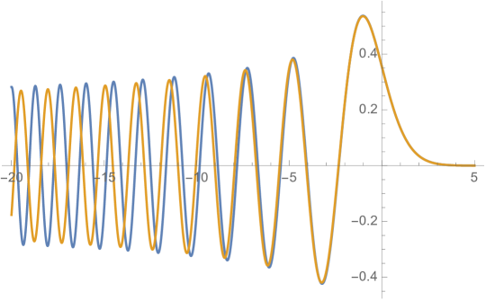
Figure 1. The Wigner function $W_{\hbar,E_{N}(\hbar)}$ of the eigenspace projection $\Pi_{\hbar,E_{N}(\hbar)}$ is always radial (see Proposition 5.1). Displayed above is the graph of the Airy function (orange) and of $W_{\hbar,E_{N}(\hbar)}$ with $N=500$ (blue) as a function of the rescaled radial variable $\rho$ in a $\hbar^{2/3}$ tube around the energy surface $H(x,\xi)=E_{N}(\hbar)=1/2.$ Theorem 5.3 predicts that, when properly scaled, $W_{\hbar,E_{N}(\hbar)}$ should converge to the Airy function (with the rate of convergence being slower farther from the energy surface, which is defined here by $\rho=0$).

5.1. Interface asymptotics for Wigner distributions of individual eigenspace projections

Our first main result gives the scaling asymptotics for the Wigner function $W_{\hbar,E_{N}(\hbar)}(x,\xi)$ of the projection onto the $E$-eigenspace of $\widehat{H}_{\hbar}$ when $(x,\xi)$ lies in an $\hbar^{2/3}$ neighborhood of the energy surface $\Sigma_{E}.$

Theorem 5.3.

Fix $E>0,d\geq 1$. Assume $E_{N}(\hbar)=E$ and let $\hbar=\hbar_{N}(E)$ (5). Suppose $(x,\xi)\in T^{*}\mathbb{R}^{d}$ satisfies

$$H(x,\xi)=E+u\left(\frac{\hbar}{2E}\right)^{2/3},\qquad u\in\mathbb{R},\,H(x,\xi)=\frac{\left\lVert x\right\rVert^{2}+\left\lVert\xi\right\rVert^{2}}{2}$$ (42)

with $\left\lvert u\right\rvert<\hbar^{-1/3}$. Then,

$$W_{\hbar,E_{N}(\hbar)}(x,\xi)=\begin{cases}\frac{2}{(2\pi\hbar)^{d}}\left(\frac{\hbar}{2E}\right)^{1/3}\left(\operatorname{Ai}(u/E)+O\left((1+\left\lvert u\right\rvert)^{1/4}u^{2}\hbar^{2/3}\right)\right),&\qquad u<0\\ \frac{2}{(2\pi\hbar)^{d}}\left(\frac{\hbar}{2E}\right)^{1/3}\operatorname{Ai}(u/E)\left(1+O\left((1+\left\lvert u\right\rvert)^{3/2}u\hbar^{2/3}\right)\right),&\qquad u>0\end{cases}$$ (43)

Here, $\operatorname{Ai}(x)$ is the Airy function. The Airy scaling of $W_{\hbar,E_{N}(\hbar)}$ is illustrated in Figure 2. The assumption (42) may be stated more invariantly that $(x,\xi)$ lies in the tube of radius $O(\hbar^{2/3})$ around $\Sigma_{E}$ defined by the gradient flow of $H$ with respect to the Euclidean metric on $T^{*}\mathbb{R}^{d}$. The asymptotics are illustrated in figure 1. Due to the behavior of the Airy function $\operatorname{Ai}(s)$, these formulae show that in the semi-classical limit $\hbar\to 0$, $E_{N}(\hbar)\to E$, $W_{\hbar,E_{N}(\hbar)}(x,\xi)$ concentrates on the energy surface surface $\Sigma_{E}$, is oscillatory inside the energy ball $\{H\leq E\}$ and is exponentially decaying outside the ball.

5.2. Interior Bessel asymptotics

In addition to the Airy asymptotics in an $\hbar^{2/3}$-tube around $\Sigma_{E}$, $W_{\hbar,E_{N}(\hbar)}$ exhibits Bessel asymptotics in the interior of $\Sigma_{E}$. There are two (or three, depending on taste) uniform asymptotic regimes for the Laguerre polynomial $L_{n}^{(\alpha)}(x)$: Bessel, Trigonometric, Airy.

For $t\in[0,1)$, define

$$A(t)=\frac{1}{2}[\sqrt{t-t^{2}}+\sin^{-1}\sqrt{t}],\;t\in[0,1].$$

For $t<0$ the $\sin^{-1}$ is replaced by $\sinh^{-1}$ and the $\frac{1}{2}$ by $i/2$ (see [FW, (2.7)]). Also, let $J_{d-1}$ be the Bessel function (of the first kind) of index $d-1$.

Theorem 5.4.

Fix $E>0$ and suppose $E_{N}(\hbar)=E.$ For each $(x,\xi)\in T^{*}\mathbb{R}^{d}$ write

$$H_{E}:=\frac{H(x,\xi)}{E}=\frac{\left\lVert x\right\rVert^{2}+\left\lVert\xi\right\rVert^{2}}{2E},\qquad\nu_{E}:=\frac{4E}{\hbar}.$$

Fix $0<a<1/2.$ Uniformly over $a\leq H_{E}\leq 1-a$, there is an asymptotic expansion,

$$W_{\hbar,E_{N}(\hbar)}(x,\xi)=\frac{2}{(2\pi\hbar)^{d}}\left[\frac{J_{d-1}(\nu_{E}A(H_{E}))}{A(H_{E})^{d-1}}\alpha_{0}(H_{E})+O\left(\nu_{E}^{-1}\left\lvert\frac{J_{d}(\nu_{E}A(H_{E}))}{A(H_{E})^{d}}\right\rvert\right)\right].$$

In particular, uniformly over $H_{E}$ in a compact subset of $(0,1),$ we find

$$W_{\hbar,E_{N}(\hbar)}(x,\xi)=(2\pi\hbar)^{-d+1/2}P_{H,E}\cos\left(\xi_{\hbar,E,H}\right)+O\left(\hbar^{-d+3/2}\right),$$ (44)

where we’ve set

$$\xi_{\hbar,E,H}=-\frac{\pi}{4}-\frac{2H}{\hbar}\left(H_{E}^{-1}-1\right)^{1/2}+\frac{2E}{\hbar}\cos^{-1}\left(H_{E}^{1/2}\right)$$

and

$$P_{E,H}:=\left(\pi E^{1/2}\left(H_{E}^{-1}-1\right)^{1/4}\left(H_{E}\right)^{d/2}\right)^{-1}.$$

5.3. Small ball integrals

The interior Bessel asymptotics do not encompass the behavior of $W_{\hbar,E_{N}(\hbar)}$ in shrinking balls around $\rho=0$. In that case, we have,

Proposition 5.5.

For $\epsilon>0$ sufficiently small and for any $a(x,\xi)\in C_{b}(T^{*}\mathbb{R}^{d})$,

$$\int_{T^{*}\mathbb{R}^{d}}a(x,\xi)W_{\hbar,E_{N}(\hbar)}(x,\xi)\psi_{\epsilon,\hbar}(x,\xi)dxd\xi=O(\hbar^{\frac{1-d}{2}-2d\epsilon}\left\lVert a\right\rVert_{L^{\infty}(B_{0}(\hbar^{1/2-\epsilon}))}).$$ (45)

where $\psi_{\epsilon,\hbar}$ is a smooth radial cut-off that is identically $1$ on the ball of radius $\hbar^{1/2-\epsilon}$ and is identically $0$ outside the ball of radius $2\hbar^{1/2-\epsilon}.$

5.4. Exterior asymptotics

If $E_{N}(\hbar)\to E$, then $W_{\hbar,E_{N}(\hbar)}(x,\xi)$ concentrates on $\Sigma_{E}$ and is exponentially decaying in the complement $H=H(x,\xi)>E$. The precise statement is,

Proposition 5.6.

Suppose that $H_{E}=H(x,\xi)/E>1$ and let $E_{N}(\hbar)=E$. Then, there exists $C_{1}>0$ so that

$$|W_{\hbar,E_{N}(\hbar)}(x,\xi)|\leq C_{1}\hbar^{-d+\frac{1}{2}}e^{-\frac{2E}{\hbar}[\sqrt{H_{E}^{2}-H_{E}}-\cosh^{-1}\sqrt{H_{E}}]}.$$

Moreover, as $H(x,\xi)\to\infty$, there exists $C_{2}>0$ so that

$$|W_{\hbar,E_{N}(\hbar)}(x,\xi)|\leq C_{2}\hbar^{-d+\frac{1}{2}}e^{-\frac{2H(x,\xi)}{\hbar}}.$$

5.5. Supremum at $\rho=0$

The reader may notice the ‘spike’ at the origin $\rho=0$; it is the point at which $W_{\hbar,E_{N}(\hbar)}$ has its global maximum (see Figure 2). The height is given by

$$\begin{array}[]{lll}W_{\hbar,E_{N}(\hbar)}(0,0)&=&\frac{(-1)^{N}}{(\pi\hbar)^{d}}L^{d-1}_{N}(0)=\frac{(-1)^{N}}{(\pi\hbar)^{d}}\frac{\Gamma(N+d)}{\Gamma(N+1)\Gamma(d)}\simeq\frac{(-1)^{N}}{\pi^{d}}C_{d}\hbar^{-d}N^{d-1}.\end{array}$$ (46)

The last statement follows from the explicit formula $L^{(d-1)}_{N}(0)=\frac{\Gamma(N+d)}{\Gamma(N+1)\Gamma(d)}=\frac{(N+d-1)!}{N!(d-1)!}$ (see e.g. [T, (1.1.39)]).

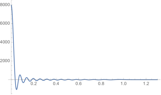
Figure 2. The Wigner function $W_{\hbar,E_{N}(\hbar)}$ of the eigenspace projection $\Pi_{\hbar,E_{N}(\hbar)}$ is always radial (see Proposition 5.1). Displayed above is the blow-up of the Wigner function at $(0,0)$.

On the complement of the ball $B(0,\hbar^{\frac{1}{2}-\epsilon})$, the Wigner distribution is much smaller than at its maximum. The following is proved by combining the estimates of Theorem 5.3 , Theorem 5.4 and Proposition 5.6.

Proposition 5.7.

For any $\epsilon>0$,

$$\sup_{(x,\xi):H(x,\xi)\geq\epsilon}|W_{\hbar,E_{N}(\hbar)}(x,\xi)|\leq C\hbar^{-d+\frac{1}{3}}.$$

The supremum in this region is achieved in $\{H\leq E\}$ at $(x,\xi)$ satisfying (42) where $u$ is the global maximum of $\rm{Ai}(x)$.

Why the spike at $\rho=0$? It is observed in [HZ19] that $W_{\hbar,E_{N}(\hbar)}$ is an eigenfunction of the (essentially isotropic) Schrödinger operator

$$\left(-\frac{\hbar^{2}}{8}(\Delta_{\xi}+\Delta_{x})+H(x,\xi)\right)W_{\hbar,E_{N}(\hbar)}=E_{N}(\hbar)W_{\hbar,E_{N}(\hbar)}.$$ (47)

on $T^{*}\mathbb{R}^{d}$. By [HZZ15, Lemma 10], the eigenspace spectral projections for the isotropic harmonic oscillator in dimension $d$ satisfies,

$$\Pi_{h,E}(x,x)=\left(2\pi h\right)^{-(d-1)}\left(2E-\left\lvert x\right\rvert^{2}\right)^{\frac{d}{2}-1}\omega_{d-1}\left(1+O(h)\right),$$

for a dimensional constant $\omega_{d}$. We apply this result to the eigenspace projections for (47) in dimension $2d$ and find that at the point $(0,0)$ its diagonal value is of order $\hbar^{-2d+1}$. We then express this eigenspace projection in terms of an orthonormal basis for the eigenspace. From the inner product formulae (16), it is seen that one of the orthonormal basis elements is $\frac{1}{\sqrt{\dim V_{\hbar,E_{N}(\hbar)}}}W_{\hbar,E_{N}(\hbar)}$. Note that ${\dim V_{\hbar,E_{N}(\hbar)}}\simeq\hbar^{-2d+1}$ in dimension $2d$. Due to the normalization and (46),

$$\frac{1}{\sqrt{\dim V_{\hbar,E_{N}(\hbar)}}}W_{\hbar,E_{N}(\hbar)}(0,0)\simeq\hbar^{-2d+1+d-\frac{1}{2}}=\hbar^{-d+\frac{1}{2}}.$$

There exists a simple spectral geometric explanation for the order of magnitude at the origin: All eigenfunctions of (47) with the exception of the radial eigenfunction $W_{\hbar,E_{N}(\hbar)}(0,0)$ vanish at the origin $(0,0)$ since they transform by non-trivial characters of $U(d)$ and $(0,0)$ is a fixed point of the action. Consequently, the value of the eigenspace projection on the diagonal at $(0,0)$ is the square of $W_{\hbar,E_{N}(\hbar)}(0,0)$ and that accounts precisely for the order of growth.

5.6. Sums of eigenspace projections

Let us begin by introducing the three types of spectral localization we are studying and the interfaces in each type.

• (i) $\hbar$-localized Weyl sums over eigenvalues in an $\hbar$-window $E_{N}(\hbar)\in[E-a\hbar,E+b\hbar]$ of width $O(\hbar)$. More generally we consider smoothed Weyl sums $W_{\hbar,E,f}$ with weights $f(\hbar^{-1}(E_{N}(\hbar)-E))$; see (49) for such $\hbar$-energy localization. This is the scale of individual spectral projections but is substantially more general than the results of [HZ19]. The scaling and asymptotics are in Theorem 5.9. For general Schrödinger operators, $\hbar$- localization around a single energy level leads to expansions in terms of periodic orbits. Since all orbits of the classical isotropic oscillator are periodic, the asymptotics may be stated without reference to them. The generalization to all Schrödinger operators will be studied in a future article.

• (ii) Airy-type $\hbar^{2/3}$-spectrally localized Weyl sums $W_{\hbar,f,2/3}(x,\xi)$ over eigenvalues in a window $[E-a\hbar^{2/3},E+a\hbar^{2/3}]$ of width $O(\hbar^{2/3})$. See Definition 5.10 for the precise definition. The levelset $\Sigma_{E}$ is viewed as the interface. The scaling asympotics of its Wigner distribution across the interface are given in Theorems 5.11 and 5.12. To our knowledge, this scaling has not previously been considered in spectral asymptotics.

• (iii) Bulk Weyl sums $\sum_{N:\hbar(N+\frac{d}{2})\in[E_{1},E_{2}]}W_{\hbar,E_{N}(\hbar)}(x,\xi)$ over energies in an $\hbar$-independent ‘window’ $[E_{1},E_{2}]$ of eigenvalues; this ‘bulk’ Weyl sum runs over $\simeq\hbar^{-1}$ distinct eigenvalues; See Definition 5.13. We are mainly interested in its scaling asymptotics around the interface $\Sigma_{E_{2}}$ (see Theorem 5.16). However, we also prove that the Wigner distribution approximates the indicator function of the shell $\{E_{1}\leq H\leq E_{2}\}\subset T^{*}\mathbb{R}^{d}$ (see Proposition 5.15). As far as we know, this is also a new result and many details are rather subtle because of oscillations inside the energy shell. Indeed, the results of [HZ19] show that the indvidual terms in the sum grow like $W_{\hbar,E_{N}(\hbar)}(x,\xi)\simeq\hbar^{-d+1/2}$ when $H(x,\xi)\in(E_{1},E_{2}).$ Proposition 5.15, in constrast, shows although the bulk Weyl sums have $\simeq\hbar^{-1}$ such terms, their sum has size $\hbar^{-d}$, implying significant cancellation.

We are particularly interested in ‘interface asymptotics’ of the Bulk Wigner-Weyl distributions $W_{\hbar,f,\delta(\hbar)}$ around the edge (i.e. boundary) of the spectral interval when $(x,\xi)$ is near the corresponding classical energy surface $\Sigma_{E}$. Such edges occur when $f$ is discontinuous, e.g. the indicator function of an interval. In other words, we integrate the empirical measures (48) below over an interval rather than against a Schwartz test function. At the interface, there is an abrupt change in the asymptotics with a conjecturally universal shape. Theorem 5.9 gives the shape of the interface for $\hbar$-localized sums, Theorem 5.11 gives the shape for $\hbar^{2/3}$ localized sums and Theorem 5.16 gives results on the bulk sums.

Our results concern asymptotics of integrals of various types of test functions against the weighted empirical measures,

$$d\mu_{\hbar}^{(x,\xi)}(\tau):=\sum_{N=0}^{\infty}W_{\hbar,E_{N}(\hbar)}(x,\xi)\delta_{E_{N}(\hbar)}(\tau),$$ (48)

and of recentered and rescaled versions of these measures (see (52) below). A key property of Wigner distributions of eigenspace projections (40) is that the measures (48) are signed, reflecting the fact that Wigner distributions take both positive and negative values, and are of infinite mass:

Proposition 5.8.

The signed measures (48) are of infinite mass (total variation norm). On the other hand, the mass of (48) is finite on any one-sided interval of the form, $[-\infty,\tau]$. Also, $\int_{\mathbb{R}}d\mu_{\hbar}^{(x,\xi)}=1$ for all $(x,\xi).$

Moreover, the $L^{2}$ norms of the terms $W_{\hbar,E_{N}(\hbar)}$ grows in $N$ like $N^{\frac{d-1}{2}}$. Hence, the measures (48) are highly oscillatory and the summands can be very large.

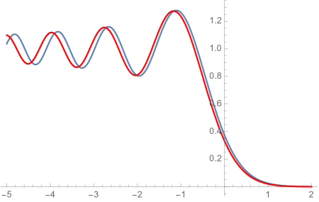
Figure 3. Plot with $\hbar\approx 0.02,\,E=1/2$ of scaled bulk Wigner-Weyl sum $(2\pi\hbar)^{d}W_{\hbar,[0,E]}(x,\xi)$ when $H(x,\xi)=E+u(\hbar/2E)^{2/3}$ as a function of $u$ (blue) against its integrated Airy limit $\int_{0}^{\infty}\mathrm{Ai}(\lambda+u/E)d\lambda$ (red) from Theorem 5.16.

5.7. Interior asymptotics for $\hbar$-localized Weyl sums

The first result we present pertains to the $\hbar$-spectrally localized Weyl sums of type (i), defined by

$$W_{\hbar,E,f}(x,\xi):=\sum_{N}f(\hbar^{-1}(E-E_{N}(\hbar)))W_{\hbar,E_{N}(\hbar)}(x,\xi),\qquad f\in\mathcal{S}(\mathbb{R}).$$ (49)

Theorem 5.9.

Fix $E>0$, and let $W_{\hbar,E,f}$ be the Wigner distribution as in (49) with $f$ an even Schwartz function. If $H(x,\xi)>E,$ then $W_{\hbar,E,f}(x,\xi)=O(\hbar^{\infty}).$ In contrast, when $0<H(x,\xi)<E$, set $H_{E}:=H(x,\xi)/E$ and define

$$t_{+,\pm,k} :=4\pi k\pm 2\cos^{-1}\left(H_{E}^{1/2}\right),\quad t_{-,\pm,k}:=4\pi\left(k+\frac{1}{2}\right)\pm 2\cos^{-1}\left(H_{E}^{1/2}\right),\qquad k\in\mathbb{Z}.$$

Fix any $\delta>0.$ Then

$$W_{\hbar,f,E}(x,\xi)=\frac{\hbar^{-d+1}\left(1+O_{\delta}(\hbar^{1-\delta})\right)}{(2E)^{1/2}(2\pi)^{d}H_{E}^{d/2}(H_{E}^{-1}-1)^{1/4}}~{}\sum_{\pm_{1},\pm_{2}\in\{+,-\}}\frac{e^{\pm_{2}i\left(\frac{\pi}{4}-\frac{4E}{\hbar}\right)}}{\left(\pm_{1}\right)^{d}}\sum_{k\in\mathbb{Z}}\widehat{f}(t_{\pm_{1},\pm_{2},k})e^{\frac{iE}{\hbar}t_{\pm_{1},\pm_{2},k}},$$

where the notation $O_{\delta}$ means the implicit constant depends on $\delta.$

Note that there are potentially an infinite number of ‘critical points’ in the support of $\hat{f}$.

5.8. Interface asymptotics for smooth $\hbar^{2/3}$-localized Weyl sums

We now consider spectrally localized Wigner distributions that are both spectrally localized and phase-space localized on the scale $\delta(\hbar)=\hbar^{2/3}$. They are mainly relevant when we study interface behavior around $\Sigma_{E}$ of Weyl sums.

Definition 5.10.

Let $H(x,\xi)=(\left\lVert x\right\rVert^{2}+\left\lVert\xi\right\rVert^{2})/2$, and assume that $(x,\xi)$ satisfiy

$$H(x,\xi)=E+u\left(\hbar/2E\right)^{2/3}.$$ (50)

Let $\delta(h)=\hbar^{2/3}$ and define the interface-localized Wigner distributions by

$$\begin{array}[]{lll}W_{\hbar,f,2/3}(x,\xi):&=&\sum_{N}f(h^{-2/3}(E-E_{N}(\hbar)))W_{\hbar,E_{N}}(x,\xi)\end{array}$$

Theorem 5.11.

Assume that $(x,\xi)$ satisfies (50) with $\left\lvert u\right\rvert<\hbar^{-2/3}.$ Fix a Schwartz function $f\in\mathcal{S}(\mathbb{R})$ with compactly supported Fourier transform. Then

$$W_{\hbar,f,2/3}(x,\xi)=(2\pi\hbar)^{-d}I_{0}(u;f,E)~{}+~{}O((1+\left\lvert u\right\rvert)\hbar^{-d+2/3}),$$

where

$$I_{0}(u;f,E)=\int_{\mathbb{R}}f(-\lambda/C_{E})\mathrm{Ai}\left(\lambda+\frac{u}{E}\right)d\lambda,\qquad C_{E}=(E/4)^{1/3}.$$

More generally, there is an asymptotic expansion

$$W_{\hbar,f,2/3}(x,\xi)~{}\simeq~{}(2\pi\hbar)^{d}\sum_{m\geq 0}\hbar^{2m/3}I_{m}\left(u;f,E\right)$$

in ascending powers of $\hbar^{2/3}$ where $I_{m}(u;f,E)$ are uniformly bounded when $u$ stays in a compact subset of $\mathbb{R}.$

The calculations show that the results are valid with far less stringent conditions on $f$ than $f\in\mathcal{S}(\mathbb{R})$ and $\widehat{f}\in C_{0}^{\infty}$. To obtain a finite expansion and remainder it is sufficient that $\int_{\mathbb{R}}|\widehat{f}(t)||t|^{k}dt<\infty$ for all $k.$ It is not necessary that $\hat{f}\in C^{k}$ for any $k>0$.

5.9. Sharp $\hbar^{2/3}$-localized Weyl sums

Next we consider the sums of Definition 5.10 when $f$ is the indicator function of a spectral interval,

$$f={\bf 1}_{[\lambda_{-},\lambda_{+}]}.$$

Equivalently, we fix integers $0<n_{{}_{\pm}}$ such that

$$\lambda_{\pm}=\hbar^{1/3}n_{\pm}~{}~{}\text{are bounded},$$

and consider the corresponding Wigner-Weyl sums $W_{\hbar,f,2/3}(x,\xi)$ of Definition 5.10:

$$W_{2/3,E,\lambda_{\pm}}(x,\xi):=\sum_{N:\,\lambda_{-}\hbar^{2/3}\leq E_{N}(\hbar)-E<\lambda_{+}\hbar^{2/3}}W_{\hbar,E_{N}(\hbar)}(x,\xi)=\sum_{N=N(E,\hbar)+n_{-}}^{N(E,\hbar)+n_{+}-1}W_{\hbar,E_{N}(\hbar)}(x,\xi),$$ (51)

where $N(E,\hbar)=E/\hbar-d/2$. Thus, the sums run over spectral intervals of size $\simeq\hbar^{2/3}$ centered at a fix $E>0$ and consist of sum of $\simeq\hbar^{-1/3}$ Wigner functions for spectral projections of individual eigenspaces. The following extends Theorem 5.11 to sharp Weyl sums at the cost of only giving a 1-term expansion plus remainder.

Theorem 5.12.

Assume that $(x,\xi)$ satisfies $\left(\left\lVert x\right\rVert^{2}+\left\lVert\xi\right\rVert^{2}\right)/2=E+u\left(\frac{\hbar}{2E}\right)^{2/3}$ with $\left\lvert u\right\rvert<\hbar^{-2/3}.$ Then,

$$W_{2/3,E,\lambda_{\pm}}(x,\xi)=(2\pi\hbar)^{-d}C_{E}\int_{-\lambda_{+}}^{-\lambda_{-}}\operatorname{Ai}\left(\frac{u}{E}+\lambda C_{E}\right)d\lambda+O\left(\hbar^{-d+1/3-\delta}+(1+\left\lvert u\right\rvert)\hbar^{-d+2/3-\delta}\right),$$

where $C_{E}=(E/4)^{1/3}.$

Theorem 5.12 can be rephrased in terms of weighted empirical measures

$$d\mu^{u,E,\frac{2}{3}}_{\hbar}:=\hbar^{d}\;\sum_{N}W_{\hbar,E_{N}(\hbar)}\left(E+u\left(\hbar/2E\right)^{2/3}\right)\delta_{[\hbar^{-2/3}(E-E_{N}(\hbar))]}.$$ (52)

obtained by centering and scaling the family (48). Thus, for $(x,\xi)$ satisfying $\left(\left\lVert x\right\rVert^{2}+\left\lVert\xi\right\rVert^{2}\right)/2=E+u\left(\frac{\hbar}{2E}\right)^{2/3},$ and for $f\in\mathcal{S}(\mathbb{R})$,

$$W_{\hbar,f,2/3}(x,\xi):=\hbar^{-d}\int_{\mathbb{R}}f(\tau)d\mu^{u,E,\frac{2}{3}}_{\hbar}(\tau),\;\;\;W_{2/3,E,\lambda_{\pm}}(x,\xi)=\hbar^{-d}\int_{\lambda_{-}}^{\lambda^{+}}d\mu^{u,E,\frac{2}{3}}_{\hbar}(\tau).$$

5.10. Bulk sums

We next consider Weyl sums of eigenspace projections corresponding to an energy shell (or window) $[E_{1},E_{2}]$. We consider both sharp and smoothed sums.

Definition 5.13.

Define the ‘bulk’ Wigner distributions for an $\hbar$-independent energy window $[E_{1},E_{2}]$ by

$$W_{\hbar,[E_{1},E_{2}]}(x,\xi):\sum_{N:E_{N}(\hbar)\in[E_{1},E_{2}]}W_{\hbar,E_{N}(\hbar)}(x,\xi).$$ (53)

More generally for $f\in C_{b}(\mathbb{R})$ define

$$W_{\hbar,f}(x,\xi):=\sum_{N=1}^{\infty}f(\hbar(N+d/2))\;W_{\hbar,E_{N}(\hbar)}(x,\xi).$$ (54)

Our first result about the bulk Weyl sums concerns the smoothed Weyl sums $W_{\hbar,f}.$

Proposition 5.14.

For $f\in\mathcal{S}(\mathbb{R})$ with $\hat{f}\in C_{0}^{\infty}$, $W_{\hbar,f}(x,\xi)$ admits a complete asymptotic expansion as $\hbar\to 0$ of the form,

$$\left\{\begin{array}[]{lll}W_{\hbar,f}(x,\xi)&\simeq&(\pi\hbar)^{-d}\sum_{j=0}^{\infty}c_{j,f,H}(x,\xi)\hbar^{j},\;\rm{with}\\ &&\\ c_{0,f,H}(x,\xi)&=&f(H(x,\xi))=\int_{\mathbb{R}}\hat{f}(t)e^{itH(x,\xi)}dt.\par\end{array}\right.$$

In general $c_{k,f,H}(x,\xi)$ is a distribution of finite order on $f$ supported at the point $(x,\xi)$.

The proof merely involves Taylor expansion of the phase.

5.11. Interior/exterior asymptotics for bulk Weyl sums of Definition 5.13

From Proposition 5.14, it is evident that the behavior of $W_{\hbar,[E_{1},E_{2}]}(x,\xi)$ depends on whether $H(x,\xi)\in(E_{1},E_{2})$ or $H(x,\xi)\notin[E_{1},E_{2}]$. Some of this dependence is captured in the following result.

Proposition 5.15.

We have,

$$W_{\hbar,[E_{1},E_{2}]}(x,\xi)=\left\{\begin{array}[]{ll}(i)\;(2\pi\hbar)^{-d}(1+O(\hbar^{1/2})),&H(x,\xi)\in(E_{1},E_{2}),\\ &\\ (ii)\;O(\hbar^{-d+1/2}),&H(x,\xi)<E_{1},\\ &\\ (iii)\;O(\hbar^{\infty}),&H(x,\xi)>E_{2}\end{array}\right.$$

The two ‘sides’ $0<H(x,\xi)<E_{1}$ and $H(x,\xi)>E_{2}$ also behave differently because the Wigner distributions have slowly decaying tails inside an energy ball but are exponentially decaying outside of it. If we write $W_{\hbar,[E_{1},E_{2}]}(x,\xi)=W_{\hbar,[0,E_{2}]}(x,\xi)-W_{\hbar,[0,E_{1}]}(x,\xi)$, we see that the two cases with $H(x,\xi)>E_{1}$ are covered by results for $W_{\hbar,[0,E]}$ with $E=E_{1}$ or $E=E_{2}$. When $H(x,\xi)<E_{1}$, then both terms of $W_{\hbar,[0,E_{2}]}(x,\xi)-W_{\hbar,[0,E_{1}]}(x,\xi)$ have the order of magnitude $\hbar^{-d}$ and the asymptotics reflect the cancellation between the terms. The boundary case where $H(x,\xi)=E_{1},$ or $H(x,\xi)=E_{2}$ is special and is given in Theorem 5.11.

5.12. Interface asymptotics for bulk Weyl sums of Definition 5.13

Our final result concerns the asymptotics of $W_{\hbar,[E_{1},E_{2}]}(x,\xi)$ in $\hbar^{\frac{2}{3}}$-tubes around the ‘interface’ $H(x,\xi)=E_{2}$. Again, it is suffcient to consider intervals $[0,E]$. It is at least intuitively clear that the interface asymptotics will depend only on the individual eigenspace projections with eigenvalues in an $\hbar^{2/3}$-interval around the energy level $E$, and since they add to $1$ away from the boundary point, one may expect the asymptotics to be similar to the interface asymptotics for individual eigenspace projections in [HZ19].

Theorem 5.16.

Assume that $(x,\xi)$ satisfies $\frac{\left\lvert x\right\rvert^{2}+\left\lvert\xi\right\rvert^{2}}{2}-E=u\left(\frac{\hbar}{2E}\right)^{2/3}$ with $\left\lvert u\right\rvert<\hbar^{-2/3}.$ Then, for any $\epsilon>0$

$$W_{\hbar,[0,E]}(x,\xi)=\left(2\pi\hbar\right)^{-d}\left[\int_{0}^{\infty}\operatorname{Ai}\left(\frac{u}{E}+\tau\right)d\tau+O(\hbar^{1/3-\epsilon}\left\lvert u\right\rvert^{1/2})+O(\left\lvert u\right\rvert^{5/2}\hbar^{2/3-\epsilon})\right],$$

where the implicit constant depends only on $d,\epsilon.$

The Airy scaling the Wigner function is illustrated in Figure 4.

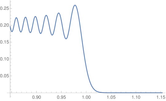
Figure 4. Scaling at energy surface of Wigner function of projection onto energy interval $[0,1/2]$.

5.13. Heuristics

Wigner distributions are normalized so that the Wigner distribution of an $L^{2}$ normalized eigenfunction has $L^{2}$ norm $1$ in $T^{*}\mathbb{R}^{d}$. Due to the multiplicity $N^{d-1}$ of eigenspaces (3), the $L^{2}$ norm of $W_{\hbar,E_{N}(\hbar)}$ is of order $N^{\frac{d-1}{2}}$.

In the main results, we sum over windows of eigenvalues, e.g. $\lambda_{-}\hbar^{2/3}\leq E-E_{N}(\hbar)<\lambda_{+}\hbar^{2/3}$ (51), resp. $E_{N}(\hbar)\in[0,E]$ in (5.13). Inevitably, the asymptotics are joint in $(\hbar,N)$. As $\hbar\downarrow 0$, the number of $N$ contributing to the sum grows at the rate $\hbar^{-\frac{1}{3}}$, resp. $\hbar^{-1}$. Due to the $N$-dependence of the $L^{2}$ norm, terms with higher $N$ have norms of higher weight in $N$ than those of small $N$ but the precise size of the contribution depends on the position of $(x,\xi)$ relative to the interface $\{H=E\}$ and of course the relation (2).

$W_{\hbar,E_{N}(\hbar)}(x,\xi)$ peaks when $H(x,\xi)=E_{N}(\hbar)$, exponentially decays in $\hbar$ when $H(x,\xi)>E_{N}(\hbar)$ and has slowly decaying tails inside the energy ball $\{H<E_{N}(\hbar)\}$, which fall into three regimes: (i) Bessel near $0$, (ii) oscillatory or trigonometric in the bulk, and (iii) Airy near $\{H=E\}.$ In terms of $N$, when (2) holds, and $H(x,\xi)<E_{N}(\hbar)$, then $W_{\hbar,E_{N}(\hbar)}(x,\xi)\simeq\hbar^{-d+1/2}\simeq N^{d-1/2}$. Near the peak point, when $H(x,\xi)-E_{N}(\hbar)\approx\hbar^{2/3}$, we have in contrast $W_{\hbar,E_{N}(\hbar)}(x,\xi)\simeq\hbar^{-d+1/3}\simeq_{E}N^{d-1/3}.$

It follows that the terms with a high value of $N$ and with $E_{N}(\hbar)\geq H(x,\xi)$ in (48) contribute high weights. There are an infinite number of such terms, and so (48) is a signed measure of infinite mass (as stated in Proposition 5.8.) This is why we mainly consider the restriction of the measures (48) to compact intervals.

5.14. Remark on nodal sets in phase space

In Section 4 we discussed nodal sets of random eigenfunctions of the isotropic Harmonic oscillator. It would also make sense to consider nodal sets in phase space $T^{*}\mathbb{R}^{d}$ for Wigner distributions $W_{\Phi_{\hbar,E}}$ of random eigenfunctions of the isotropic Harmonic oscillator. This is of interest because Wigner distributions are signed, i.e. not positive, and their nodal sets and domains signal the extent of this ‘defect’ in their interpretation as phase space densities. But so far, this has not been done. However, the covariance function is simply the Wigner distribution of the spectral projection kernels, so the analysis of Wigner distributions and of their interfaces across energy surfaces provides the necessary techniques.

In the next section we consider interfaces for partial Bergman kernels. The analogue in the complex domain of random nodal sets of isotropic oscillator eigenfunctions is zero sets of random homogeneous holomorphic polynomials of fixed degree in $\mathbb{C}^{d}$. This is essentially the same as studying such zero sets on complex projective space $\mathbb{CP}^{d-1}$, and to that extent the theory has already been developed. But interface phenomena for complex zero sets has not so far been studied.

6. Interfaces in phase space: partial Bergman kernels

In this section, we continue to study phase space distributions of orthogonal projections, but change from the Schrödinger quantization to the holomorphic quantization. The holomorphic setting consists of Berezin-Toeplitz operators acting on holomorphic sections of line bundles over Kähler manifolds, and is analytically simpler than the real Schrödinger setting. Hence we are able to present much more general results. Instead of fixing a model Schrödinger operator like the isotropic Harmonic Oscillator, we consider all possible Toeplitz Hamiltonians on holomorphic sections of Hermitian line bundles $(L,h)\to(M,\omega)$ over all possible projective Kähler manifolds. Here it is assumed that $i\partial\overline{\partial}\log h=\omega$, i.e. that $(L,h)$ is a positive, ample line bundle. For background on Bargmann-Fock space, and on line bundles over general Kähler manifolds, we refer to Section 10.

Motivation to study partial Bergman kernels comes from two sources. On the one hand, they arise in many problems of complex geometry (see [Ber1, HW17, HW18, PS, RS] besides the articles surveyed here). On the other hand, they arise in the IQHE (integer quantum Hall effect). The author’s interest was stimulated by conversations with A. Abanov, S. Klevtsov and P. Wiegmann during a Simons’ Center program on complex geometry and the IQHE. We refer to [W, Wieg, CFTW] for some physics articles where interfaces in the density of states of the IQHE are studied. It should be emphasized that there are many types of partial Bergman kernels, and the ones most interesting in physics are still out of reach of the rigorous techniques described here. What we study here are spectral partial Bergman kernels, i.e. orthogonal projection kernels onto spectral subspaces for Toeplitz Hamiltonians. By no means do all pBK’s (partial Bergman kernels) arise from spectral problems, but the spectral pBK’s are the only types for which there exist general results (or almost any results) and sometimes the pBK’s of interest in the IQHE are spectral pBK’s.

We do not review the basic definitions here (see Section 10) but head straight for the interface results. In place of the spectral projections of the previous sections, we consider partial Bergman kernels on “polarized” Kähler manifolds $(L,h)\to(M^{m},\omega,J)$, i.e. Kähler manifolds of (complex) dimension $m$ equipped with a Hermitian holomorphic line bundle whose curvature form $F_{\nabla}$ for the Chern connection $\nabla$ satisfies $\omega=iF_{\nabla}$. Partial Bergman kernels

$$\Pi_{k,\mathcal{S}_{k}}:L^{2}(M,L^{k})\to\mathcal{S}_{k}\subset H^{0}(M,L^{k})$$ (55)

are Schwarz kernels for orthogonal projections onto proper subspaces $\mathcal{S}_{k}$ of the holomorphic sections of $L^{k}$.

For general subspaces, there is little one can say about the asymptotics of the partial density of states $\Pi_{k,\mathcal{S}_{k}}(z)$, i.e. the contraction of the diagonal of the kernel. But for certain sequences $\mathcal{S}_{k}$ of subspaces, the partial density of states $\Pi_{k,\mathcal{S}_{k}}(z)$ has an asymptotic expansion as $k\to\infty$ which roughly gives the probability density that a quantum state from $\mathcal{S}_{k}$ is at the point $z$. More concretely, in terms of an orthonormal basis $\{s_{i}\}_{i=1}^{N_{k}}$ of $\mathcal{S}_{k}$, the partial Bergman densities defined by

$$\Pi_{k,\mathcal{S}_{k}}(z)=\sum_{i=1}^{N_{k}}\|s_{i}(z)\|^{2}_{h^{k}}.$$ (56)

When $\mathcal{S}_{k}=H^{0}(M,L^{k})$, $\Pi_{k,\mathcal{S}_{k}}=\Pi_{k}:L^{2}(M,L^{k})\to H^{0}(M,L^{k})$ is the orthogonal (Szegö or Bergman) projection. We also call the ratio $\frac{\Pi_{k,\mathcal{S}_{k}}(z)}{\Pi_{k}(z)}$ the partial density of states.

Corresponding to $\mathcal{S}_{k}$ there is an allowed region $\mathcal{A}$ where the relative partial density of states $\Pi_{k,\mathcal{S}_{k}}(z)/\Pi_{k}(z)$ is one, indicating that the states in $\mathcal{S}_{k}$ “fill up” $\mathcal{A}$, and a forbidden region $\mathcal{F}$ where the relative density of states is $O(k^{-\infty})$, indicating that the states in $\mathcal{S}_{k}$ are almost zero in $\mathcal{F}$. On the boundary $\mathcal{C}:=\partial\mathcal{A}$ between the two regions there is a shell of thickness $O(k^{-\frac{1}{2}})$ in which the density of states decays from $1$ to $0$. The $\sqrt{k}$-scaled relative partial density of states is asymptotically Gaussian along this interface, in a way reminiscent of the central limit theorem. This was proved in [RS] for certain Hamiltonian holomorphic $S^{1}$ actions, then in greater generality in [ZZ17]. In fact, it is a universal property of partial Bergman kernels defined by $C^{\infty}$ Hamiltonians.

To begin with, we define the subspaces $\mathcal{S}_{k}$. They are defined as spectral subspaces for the quantization of a smooth function $H:M\to\mathbb{R}$. By the standard (Kostant) method of geometric quantization, one can quantize $H$ as the self-adjoint zeroth order Toeplitz operator

$${H}_{k}:=\Pi_{k}(\frac{i}{k}\nabla_{\xi_{H}}+H)\Pi_{k}:H^{0}(M,L^{k})\to H^{0}(M,L^{k})$$ (57)

acting on the space $H^{0}(M,L^{k})$ of holomorphic sections. Here, $\xi_{H}$ is the Hamiltonian vector field of $H$, $\nabla_{\xi_{H}}$ is the Chern covariant deriative on sections, and $H$ acts by multiplication. We denote the eigenvalues (repeated with multiplicity) of $\hat{H}_{k}$ (57) by

$$\mu_{k,1}\leq\mu_{k,2}\leq\cdots\leq\mu_{k,N_{k}},$$ (58)

where $N_{k}=\dim H^{0}(M,L^{k})$, and the corresponding orthonormal eigensections in $H^{0}(M,L^{k})$ by $s_{k,j}$.

Let $E$ be a regular value of $H$. We denote the partial Bergman kernels for the corresponding spectral subspaces by

$$\Pi_{k,E}:H^{0}(M,L^{k})\to\mathcal{H}_{k,E},$$ (59)

where

$$\mathcal{S}_{k}:=\mathcal{H}_{k,E}:=\bigoplus_{\mu_{k,j}<E}V_{\mu_{k,j}},$$ (60)

$\mu_{k,j}$ being the eigenvalues of ${H}_{k}$ and

$$V_{\mu_{k,j}}:=\{s\in H^{0}(M,L^{k}):{H}_{k}s=\mu_{k,j}s\}.$$ (61)

We denote by $\Pi_{k,j}:H^{0}(M,L^{k})\to V_{\mu_{k,j}}$ the orthogonal projection to $V_{\mu_{k,j}}$. The associated allowed region $\mathcal{A}$ is the classical counterpart to (60), and the forbidden region $\mathcal{F}$ and the interface $\mathcal{C}$ are

$$\mathcal{A}:=\{z:H(z)<E\},\quad\mathcal{F}=\{z:H(z)>E\},\quad\mathcal{C}=\{z:H(z)=E\}.$$ (62)

More generally, for any spectral interval $I\subset\mathbb{R}$ we define the partial Bergman kernels to be the orthogonal projections,

$$\Pi_{k,I}:H^{0}(M,L^{k})\to\mathcal{H}_{k,I},$$ (63)

onto the spectral subspace,

$$\mathcal{H}_{k,I}:=\text{span}\{s_{k,j}:\mu_{k,j}\in I\}$$ (64)

Its (Schwartz) kernel is defined by

$$\Pi_{k,I}(z,w)=\sum_{\mu_{k,j}\in I}s_{k,j}(z)\overline{s_{k,j}(w)}.$$ (65)

and the metric contraction of (65) on the diagonal with respect to $h^{k}$ is the partial density of states,

$$\Pi_{k,I}(z)=\sum_{\mu_{k,j}\in I}\|s_{k,j,\alpha}(z)\|^{2}.$$

The classical allowed region $\mathcal{A}$ and forbidden region $\mathcal{F}$ are the open subsets

$$\mathcal{A}:=\text{Int}(H^{-1}(I)),\quad\mathcal{F}=\text{Int}(M\backslash\mathcal{A}),$$

and the interface as

$$\mathcal{C}=\partial\mathcal{A}=\partial\mathcal{F}.$$

In [ZZ17] it is proved that

$$\frac{\Pi_{k,I}(z)}{\Pi_{k}(z)}=\begin{cases}1&\text{if }z\in\mathcal{A}\\ 0&\text{if }z\in\mathcal{F}\end{cases}\mod O(k^{-\infty}),$$

We denote by $\Pi_{k}(z,w)$ and $\Pi_{k}(z)$ the (full) Bergman kernel and density function. Here and throughout, we use the notation $K(z)$ for the metric contraction of the diagonal values $K(z,z)$ of a kernel.

For each $z\in\mathcal{C}$, let $\nu_{z}$ be the unit normal vector to $\mathcal{C}$ pointing towards $\mathcal{A}$. And let $\gamma_{z}(t)$ be the geodesic curve with respect to the Riemannian metric $g(X,Y)=\omega(X,JY)$ defined by the Kähler form $\omega$, such that $\gamma_{z}(0)=z,\dot{\gamma}_{z}(0)=\nu_{z}$. For small enough $\delta>0$, the map

$$\Phi:\mathcal{C}\times(-\delta,\delta)\to M,\quad(z,t)\mapsto\gamma_{z}(t)$$ (66)

is a diffeomorphism onto its image.

Main Theorem.

Let $(L,h)\to(M,\omega,J)$ be a polarized Kähler manifold. Let $H:M\to\mathbb{R}$ be a smooth function and $E$ a regular value of $H$. Let $\mathcal{S}_{k}\subset H^{0}(X,L^{k})$ be defined as in (60). Then we have the following asymptotics on partial Bergman densities $\Pi_{k,\mathcal{S}_{k}}(z)$:

$$\left(\frac{\Pi_{k,\mathcal{S}_{k}}}{\Pi_{k}}\right)(z)=\begin{cases}1&\text{if }z\in\mathcal{A}\\ 0&\text{if }z\in\mathcal{F}\end{cases}\mod O(k^{-\infty}).$$

For small enough $\delta>0$, let $\Phi:\mathcal{C}\times(-\delta,\delta)\to M$ be given by (66). Then for any $z\in\mathcal{C}$ and $t\in\mathbb{R}$, we have

$$\left(\frac{\Pi_{k,\mathcal{S}_{k}}}{\Pi_{k}}\right)(\Phi(z,t/\sqrt{k}))=\operatorname{Erf}(2\sqrt{\pi}t)+O(k^{-1/2}),$$ (67)

where $\operatorname{Erf}(x)=\int_{-\infty}^{x}e^{-s^{2}/2}\frac{ds}{\sqrt{2\pi}}$ is the cumulative distribution function of the Gaussian, i.e., $\mathbb{P}_{X\sim N(0,1)}(X<x)$.

rem 6.1.

The analogous result for critical levels is proved in [ZZ18b]. We could also choose an interval $(E_{1},E_{2})$ with $E_{i}$ regular values of $H$, and define $\mathcal{S}_{k}$ as the span of eigensections with eigenvalue within $(E_{1},E_{2})$. However the interval case can be deduced from the half-ray case $(-\infty,E)$ by taking difference of the corresponding partial Bergman kernel, hence we only consider allowed region of the type in (62).

Example 6.2.

As a quick illustration, holomorphic sections of the trivial line bundle over $\mathbb{C}$ are holomorphic functions on $\mathbb{C}$. We equip the bundle with the Hermitian metric where $1$ has the norm-square $e^{-|z|^{2}}$. The $k$th power has metric $e^{-k|z|^{2}}$ Fix $\epsilon>0$ and define the subspaces $\mathcal{S}_{k}=\oplus_{j\leq\epsilon k}z^{j}$ of sections vanishing to order at most $\epsilon k$ at $0$, or sections with eigenvalues $\mu<\epsilon$ for operator $H_{k}=\frac{1}{ik}\partial_{\theta}$ quantizing $H=|z|^{2}$. The full and partial Bergman densities are

$$\Pi_{k}(z)=\frac{k}{2\pi},\quad\Pi_{k,\epsilon}(z)=\left(\frac{k}{2\pi}\right)\sum_{j\leq\epsilon k}\frac{k^{j}}{j!}|z^{j}|^{2}e^{-k|z|^{2}},$$

As $k\to\infty$, we have

$$\lim_{k\to\infty}k^{-1}\Pi_{k,\epsilon}(z)=\begin{cases}1&|z|^{2}<\epsilon\\ 0&|z|^{2}>\epsilon.\end{cases}$$

For the boundary behavior, one can consider sequence $z_{k}$, such that $|z_{k}|^{2}=\epsilon(1+k^{-1/2}u),$

$$\lim_{k\to\infty}k^{-1}\Pi_{k,\epsilon}(z_{k})=\operatorname{Erf}(u).$$

This example is often used to illustrate the notion of ‘filling domains’ in the IQH (integer Quantum Hall) effect. In IQH, one considers a free electron gas confined in plane $\mathbb{R}^{2}\simeq\mathbb{C}$, with a uniform magnetic field in the perpendicular direction. A one-particle electron state is said to be in the lowest Landau level (LLL) if it has the form $\Psi(z)=e^{-|z|^{2}/2}f(z)$, where $f(z)$ is holomorphic as in Example 6.2. The following image of the density profile is copied from [W], where the picture on the right illustrates how the states $\frac{(\sqrt{k}\;z)^{j}}{\sqrt{j!}}e^{-k|z|^{2}/2}$ with $j\leq\epsilon k$ fill the disc of radius $\sqrt{\epsilon}$, so that the density profile drops from $1$ to $0$.

Figure 5. “The density profile of the $\nu=1$ droplet, where the first $m$ levels (represented by the thick lines) are filled.” From Fig 7.11 in [W].

The example is $S^{1}$ symmetric and therefore the simpler results of [ZZ16] apply. For more general domains $D\subset\mathbb{C}$, it is not obvious how to fill $D$ with LLL states. The Main Theorem answers the question when $D=\{H\leq E\}$ for some $H$. For a physics discussion of Erf asymptotics and their (as yet unknown) generalization to the fractional QH effect, see [Wieg, CFTW].

6.1. Three families of measures at different scales

The rationale for viewing the Erf asymptotics of scaled partial Bergman kernels along the interface $\mathcal{C}$ is explained by considering three different scalings of the spectral problem.

$$\left\{\begin{array}[]{ll}(i)&d\mu_{k}^{z}(x)\;\;=\sum_{j}\Pi_{k,j}(z)\delta_{\mu_{k,j}}(x),\\ &\\ (ii)&d\mu^{z,\frac{1}{2}}_{k}(x)=\sum_{j}\Pi_{k,j}(z)\delta_{\sqrt{k}(\mu_{k,j}-H(z))}(x),\\ &\\ (iii)&d\mu^{z,1,\tau}_{k}(x)=\sum_{j}\Pi_{k,j}(z)\delta_{k(\mu_{k,j}-H(z))+\sqrt{k}\tau}(x),\end{array}\right.$$ (68)

where as usual, $\delta_{y}$ is the Dirac point mass at $y\in\mathbb{R}$. We use $\mu(x)=\int_{-\infty}^{x}d\mu(y)$ to denote the cumulative distribution function.

We view these scalings as analogous to three scalings of the convolution powers $\mu^{*k}$ of a probability measure $\mu$ supported on $[-1,1]$ (say). The third scaling (iii) corresponds to $\mu^{*k}$, which is supported on $[-k,k]$. The first scaling (i) corresponds to the Law of Large Numbers, which rescales $\mu^{*k}$ back to $[-1,1]$. The second scaling (ii) corresponds to the CLT (central limit theorem) which rescales the measure to $[-\sqrt{k},\sqrt{k}]$.

Our main results give asymptotic formulae for integrals of test functions and characteristic functions against these measures. To obtain the remainder estimate (67), we need to apply semi-classical Tauberian theorems to $\mu^{z,\frac{1}{2}}_{k}$ and that forces us to find asymptotics for $\mu^{z,1,\tau}_{k}$.

6.2. Unrescaled bulk results on $d\mu_{k}^{z}$

The first result is that the behavior of the partial density of states in the allowed region $\{z:H(z)<E\}$ is essentially the same as for the full density of states, while it is rapidly decaying outside this region.

We begin with a simple and general result about partial Bergman kernels for smooth metrics and Hamiltonians.

Theorem 1.

Let $\omega$ be a $C^{\infty}$ metric on $M$ and let $H\in C^{\infty}(M)$. Fix a regular value $E$ of $H$ and let $\mathcal{A},\mathcal{F},\mathcal{C}$ be given by (62). Then for any $f\in C^{\infty}(\mathbb{R})$, we have

$$\Pi_{k}(z)^{-1}\int_{-\infty}^{E}f(\lambda)d\mu_{k}^{z}(\lambda)\to\begin{cases}f(H(z))&\rm{if}z\in\mathcal{A}\\ 0&\rm{if}z\in\mathcal{F}.\\ \end{cases}$$ (69)

In particular, the density of states of the partial Bergman kernel is given by the asymptotic formula:

$$\Pi_{k}(z)^{-1}\Pi_{k,E}(z)\sim\begin{cases}1\mod O(k^{-\infty})&\rm{if}z\in\mathcal{A}\\ 0\mod O(k^{-\infty})&\rm{if}z\in\mathcal{F}.\\ \end{cases}$$ (70)

where the asymptotics are uniform on compact sets of $\mathcal{A}$ or $\mathcal{F}.$

In effect, the leading order asymptotics says that the normalized measure $\Pi_{k}(z)^{-1}d\mu_{k}^{z}\to\delta_{H(z)}$. This is a kind of Law of Large Numbers for the sequence $d\mu_{k}^{z}$. The theorem does not specify the behavior of $\mu_{k}^{z}(-\infty,E)$ when $H(z)=E$. The next result pertains to the edge behavior.

6.3. $\sqrt{k}$-scaling results on $d\mu^{z,1/2}_{k}$

The most interesting behavior occurs in $k^{-\frac{1}{2}}$-tubes around the interface $\mathcal{C}$ between the allowed region $\mathcal{A}$ and the forbidden region $\mathcal{F}$. For any $T>0$, the tube of ‘radius’ $Tk^{-\frac{1}{2}}$ around $\mathcal{C}=\{H=E\}$ is the flowout of $\mathcal{C}$ under the gradient flow of $H$

$$F^{t}:=\exp(t\nabla H):M\to M,$$

for $|t|<Tk^{-1/2}$. Thus it suffices to study the partial density of states $\Pi_{k,E}(z_{k})$ at points $z_{k}=F^{\beta/\sqrt{k}}(z_{0})$ with $z_{0}\in H^{-1}(E).$ The interface result for any smooth Hamiltonian is the same as if the Hamiltonian flow generate a holomorphic $S^{1}$-actions, and thus our result shows that it is a universal scaling asymptotics around $\mathcal{C}$.

Theorem 2.

Let $\omega$ be a $C^{\infty}$ metric on $M$ and let $H\in C^{\infty}(M)$. Fix a regular value $E$ of $H$ and let $\mathcal{A},\mathcal{F},\mathcal{C}$ be given by (62). Let $F^{t}:M\to M$ denote the gradient flow of $H$ by time $t$. We have the following results:

1. For any point $z\in\mathcal{C}$, any $\beta\in\mathbb{R}$, and any smooth function $f\in C^{\infty}(\mathbb{R})$, there exists a complete asymptotic expansion,

   $$\sum_{j}f(\sqrt{k}(\mu_{k,j}-E))\Pi_{k,j}(F^{\beta/\sqrt{k}}(z))\simeq\left(\frac{k}{2\pi}\right)^{m}(I_{0}+k^{-\frac{1}{2}}I_{1}+\cdots),$$ (71)

   in descending powers of $k^{\frac{1}{2}}$, with the leading coefficient as

   $$I_{0}(f,z,\beta)=\int_{-\infty}^{\infty}f(x)e^{-\left(\frac{x}{|\nabla H|(z)|}-\beta|\nabla H(z)|\right)^{2}}\frac{dx}{\sqrt{\pi}|\nabla H(z)|}.$$

2. For any point $z\in\mathcal{C}$, and any $\alpha\in\mathbb{R}$, the cumulative distribution function $\mu^{z,1/2}_{k}(\alpha)=\int_{-\infty}^{\alpha}d\mu^{z,1/2}_{k}$ is given by

   $$\mu^{z,1/2}_{k}(\alpha)=\sum_{\mu_{k,j}<E+\frac{\alpha}{\sqrt{k}}}\Pi_{k,j}(z)=\left(\frac{k}{2\pi}\right)^{m}\operatorname{Erf}\left(\frac{\sqrt{2}\alpha}{|\nabla H(z)|}\right)+O(k^{m-1/2}).$$ (72)

3. For any point $z\in\mathcal{C}$, and any $\beta\in\mathbb{R}$, the Bergman kernel density near the interface is given by

   $$\Pi_{k,E}(F^{\beta/\sqrt{k}}(z))=\sum_{\mu_{j,k}<E}\Pi_{k,j}(F^{\beta/\sqrt{k}}(z))=\left(\frac{k}{2\pi}\right)^{m}\operatorname{Erf}\left(-\sqrt{2}\beta|\nabla H(z)|\right)+O(k^{m-1/2}).$$ (73)

rem 6.3.

The leading power $\left(\frac{k}{2\pi}\right)^{m}$ is the same as in Theorem 1, despite the fact that we sum over a packet of eigenvalues of width (and cardinality) $k^{-\frac{1}{2}}$ times the width (and cardinality) in Theorem 1. This is because the summands $\Pi_{k,j}(z)$ already localize the sum to $\mu_{k,j}$ satisfying $|\mu_{k,j}-H(z)|<Ck^{-\frac{1}{2}}$.

6.4. Energy level localization and $d\mu^{z,1,\alpha}_{k}$

To obtain the remainder estimate for the $\sqrt{k}$ rescaled measure $d\mu^{z,1/2}_{k}$ in (72) and (73) , we apply the Tauberian theorem. Roughly speaking, one approximate $d\mu^{z,1/2}_{k}$ by convoluting the measure with a smooth function $W_{h}$ of width $h$, and the difference of the two is proportional to $h$. The smoothed measure $d\mu^{z,1/2}_{k}*W_{h}$ has a density function, the value of which can be estimated by an integral of the propagator $U_{k}(t,z,z)$ for $|t|\sim k^{-1}/(hk^{-1/2})$. Thus if we choose $h=k^{-1/2}$, and $W_{h}$ to have Fourier transform supported in $(-\epsilon,+\epsilon)/h$, we only need to evaluted $U_{k}(t,z,z)$ for $|t|<\epsilon$, where $\epsilon$ can be taken to be arbitrarily small.

Theorem 3.

Let $E$ be a regular value of $H$ and $z\in H^{-1}(E)$. If $\epsilon$ is small enough, such that the Hamiltonian flow trajectory starting at $z$ does not loop back to $z$ for time $|t|<2\pi\epsilon$, then for any Schwarz function $f\in\mathcal{S}(\mathbb{R})$ with $\hat{f}$ supported in $(-\epsilon,\epsilon)$ and $\hat{f}(0)=\int f(x)dx=1$, and for any $\alpha\in\mathbb{R}$ we have

$$\int_{\mathbb{R}}f(x)d\mu^{z,1,\alpha}_{k}(x)=\left(\frac{k}{2\pi}\right)^{m-1/2}e^{-\frac{\alpha^{2}}{\|\xi_{H}(z)\|^{2}}}\frac{\sqrt{2}}{2\pi\|\xi_{H}(z)\|}(1+O(k^{-1/2})).$$

6.5. Critical levels

In this section we consider interfaces at critical levels. Let $H:M\to\mathbb{R}$ be a smooth function with Morse critical points.Henceforth, to simplify notation, we use Kähler local coordinates $u$ centered at $z_{0}$ to write points in the $k^{-\epsilon}$ tube around $\mathcal{C}$ by

$$z=z_{0}+k^{-\epsilon}u:=\exp_{z_{0}}(k^{-\epsilon}u),\quad u\in T_{z_{0}}.\mathcal{C}$$

The abuse of notation in dropping the higher order terms of the normal exponential map is harmless since we are working so close to $\mathcal{C}$. At regular points $z_{0}$ we may use the exponential map along $N_{z_{0}}\mathcal{C}$ but we also want to consider critical points. More generally we write $z_{0}+u$ for the point with Kähler normal coordinate $u$. In these coordinates,

$$\omega(z_{0}+u)=i\sum_{j=1}^{m}du_{j}\wedge d\bar{u}_{j}+O(|u|).$$

We also choose a local frame $e_{L}$ of $L$ near $z$, such that the corresponding $\varphi=-\log h(e_{L},e_{L})$ is given by

$$\varphi(z_{0}+u)=|u|^{2}+O(|u|^{3}).$$

See [ZZ17] for more on such adapted frames and Heisenberg coordinates.

Clearly, the formula (71) breaks down at critical points and near such points on critical levels. Our main goal in this paper is to generalize the interface asymptotics to the case when the Hamiltonian is a Morse function and the interface $\mathcal{C}=\{H=E\}$ is a critical level, so that $\mathcal{C}$ contains a non-degenerate critical point $z_{c}$ of $H$. To allow for non-standard scaling asymptotics, we study the smoothed partial Bergman density near the critical value $E=H(z_{c})$,

$$\Pi_{k,E,f,\delta}(z):=\sum_{j}\|s_{k,j}(z)\|^{2}\cdot f(k^{\delta}(\mu_{k,j}-E))$$

where $f\in\mathcal{S}(\mathbb{R})$ with Fourier transform $\hat{f}\in C^{\infty}_{c}(\mathbb{R})$, and $0\leq\delta\leq 1$. This is the smooth analog of summing over eigenvalues within $[E-k^{-\delta},E+k^{-\delta}]$.

The behavior of the scaled density of states is encoded in the following measures,

$$\left\{\begin{array}[]{l}d\mu_{k}^{z}(x)=\sum_{j}\|s_{k,j}(z)\|^{2}\,\delta_{\mu_{k,j}}(x),\\ \\ d\mu_{k}^{z,\delta}(x)=\sum_{j}\|s_{k,j}(z)\|^{2}\,\delta_{k^{\delta}(\mu_{k,j}-H(z))}(x),\\ \\ d\mu_{k}^{(z,u,\epsilon),\delta}(x)=\sum_{j}\|s_{k,j}(z+k^{-\epsilon}u)\|^{2}\,\delta_{k^{\delta}(\mu_{k,j}-H(z))}(x).\end{array}\right.$$ (74)

For each measure $\mu$ we denote by $d\hat{\mu}$ the normalized probability measure

$$d\hat{\mu}(x)=\mu(\mathbb{R})^{-1}d\mu(x).$$

For all $z\in M$, we have the following weak limit, reminiscent of the law of large numbers;

$$\hat{\mu}_{k}^{z}(x)\rightharpoonup\delta_{H(z)}(x).$$

For $z\in M$ with $dH(z)\neq 0$, (71) shows that

$$\hat{\mu}_{k}^{z,1/2}(x)\rightharpoonup e^{-\frac{x^{2}}{|dH(z)|^{2}}}\frac{dx}{\sqrt{\pi}|dH(z)|}.$$

6.6. Interface asymptotics at critical levels

The next result generalizes the ERF scaling asymptotics to the critical point case. We use the following setup: Let $z_{c}$ be a non-degenerate Morse critical point of $H$, then for small enough $u\in\mathbb{C}^{m}$, we denote the Taylor expansion components by

$$H(z_{c}+u)=E+H_{2}(u)+O(|u|^{3}).$$

where

$$E=H(z_{c}),\quad H_{2}(u)=\frac{1}{2}{\operatorname{Hess}}_{z_{c}}H(u,u).$$

Theorem 6.4.

For any $f\in\mathcal{S}(\mathbb{R})$ with $\hat{f}\in C^{\infty}_{c}(\mathbb{R})$, we have

$$\Pi_{k,E,f,1/2}(z_{c}+k^{-1/4}u):=\sum_{j}\|s_{k,j}(z_{c}+k^{-1/4}u)\|^{2}\cdot f(k^{1/2}(\mu_{k,j}-E))=\left(\frac{k}{2\pi}\right)^{m}f(H_{2}(u))+O_{f}(k^{m-1/4}).$$

More over, the normalized rescaled pointwise spectral measure

$$d\hat{\mu}_{k}^{(z_{c},u,1/4),1/2}(x):=\frac{\sum_{j}\|s_{k,j}(z_{c}+k^{-1/4}u)\|^{2}\,\delta_{k^{1/2}(\mu_{k,j}-E)}(x)}{\sum_{j}\|s_{k,j}(z_{c}+k^{-1/4}u)\|^{2}}$$

converges weakly

$$\hat{\mu}_{k}^{(z_{c},u,1/4),1/2}(x)\rightharpoonup\delta_{H_{2}(u)}(x).$$

We notice that the scaling width has changed from $k^{-\frac{1}{2}}$ to $k^{-1/4}$ due to the critical point. The difference in scalings raises the question of what happens if we scale by $k^{-\frac{1}{2}}$ around a critical point. The result is stated in terms of the metaplectic representation on the osculating Bargmann-Fock space at $z_{c}$.

Theorem 6.5.

Let $1\gg T>0$ be small enough, such that there is no non-constant periodic orbit with periods less than $T$. Then for any $f\in\mathcal{S}(\mathbb{R})$ with $\hat{f}\in C^{\infty}_{c}((-T,T))$, we have

$$\Pi_{k,E,f,1}(z_{c}+k^{-1/2}u)=\left(\frac{k}{2\pi}\right)^{m}\int_{\mathbb{R}}\hat{f}(t)\mathcal{U}(t,u)\frac{dt}{2\pi}+O(k^{m-1/2})$$

where $\mathcal{U}(t,u)$ is the metaplectic quantization of the Hamiltonian flow of $H_{2}(u)$ defined as

$$\mathcal{U}(t,u)=(\det P)^{-1/2}\exp(\bar{u}(P^{-1}-1)u+u\bar{Q}P^{-1}u/2-\bar{u}P^{-1}Q\bar{u}/2).$$

Here $P=P(t),Q=Q(t)$ be complex $m\times m$ matrices such that if $u(t)=\exp(t\xi_{H_{2}})u$, then

$$\begin{pmatrix}u(t)\\ \bar{u}(t)\end{pmatrix}=\begin{pmatrix}P(t)&Q(t)\\ \bar{Q}(t)&\bar{P}(t)\end{pmatrix}\begin{pmatrix}u\\ \bar{u}\end{pmatrix}.$$

rem 6.6.

Unlike the universal $\operatorname{Erf}$ decay profile in the $1/\sqrt{k}$-tube around the smooth part of $\mathcal{C}$, we cannot give the decay profile of $\Pi_{k,I}(z)$ near the critical point $z_{c}$. The reason is that there are eigensections that highly peak near $z_{c}$ and with eigenvalues clustering around $H(z_{c})$. Hence it even matters whether we use $[E_{1},E_{2}]$ or $(E_{1},E_{2})$. See the following case where the Hamiltonian action is holomorphic, where the peak section at $z_{c}$ is an eigensection, and all other eigensections vanishes at $z_{c}$.

The next result pertains to Hamiltonians generating $\mathbb{R}$ actions, as studied in [RS, ZZ16]. The Hamiltonian flow always extends to a holomorphic $\mathbb{C}$ action.

Proposition 6.7.

Assume $H$ generate a holomorphic Hamiltonian $\mathbb{R}$ action. The pointwise spectral measure $d\mu_{k}^{z_{c}}(x)$ is always a delta-function

$$\mu_{k}^{z_{c}}=\delta_{H(z_{c})}(x),\quad\forall k=1,2\cdots$$

Equivalently, for any spectral interval $I$,

$$\lim_{k\to\infty}\Pi_{k,I}(z_{c})=\begin{cases}1&E\in I\\ 0&E\notin I\end{cases}.$$

The above result follows immediately from:

Proposition 6.8.

Let $z_{c}$ be a Morse critical point of $H$, $E=H(z_{c})$. Then

1. The $L^{2}$-normalized peak section $s_{k,z_{c}}(z)=C(z_{c})\Pi_{k}(z,z_{c})$ is an eigensection of $\hat{H}_{k}$ with eigenvalue $H(z_{c})$. And all other eigensections orthogonal to $s_{k,z_{c}}$ vanishes at $z_{c}$.

2. If $s_{k,j}\in H^{0}(M,L^{k})$ is an eigensection of $\hat{H}_{k}$ with eigenvalue $\mu_{k,j}<E$, then $s_{k,j}$ vanishes on $W^{+}(z_{c})$.

3. If $s_{k,j}\in H^{0}(M,L^{k})$ is an eigensection of $\hat{H}_{k}$ with eigenvalue $\mu_{k,j}>E$, then $s_{k,j}$ vanishes on $W^{-}(z_{c})$.

In particular, this shows the concentration of eigensection near $z_{c}$. Depending on whether the spectral inteval $I$ includes boundary point $H(z_{c})$ or not, the partial Bergman density will differ by a large Gaussian bump of height $\sim k^{m}$.

6.7. Sketch of Proof

As in [ZZ17, ZZ18] the proofs involve rescaling parametrices for the propagator

$$U_{k}(t)=\exp itk\hat{H}_{k}$$ (75)

of the Hamiltonian (57). The parametrix construction is reviewed in Section 3.4. We begin by observing that for all $z\in M$, the time-scaled propagator has pointwise scaling asymptotics with the $k^{-\frac{1}{2}}$ scaling:

Proposition 6.9 ([ZZ17] Proposition 5.3).

If $z\in M$, then for any $\tau\in\mathbb{R}$,

$$\hat{U}_{k}(t/\sqrt{k},\hat{z},\hat{z})=\left(\frac{k}{2\pi}\right)^{m}e^{it\sqrt{k}H(z)}e^{-t^{2}\frac{\|dH(z)\|^{2}}{4}}(1+O(|t|^{3}k^{-1/2})),$$

where the constant in the error term is uniform as $t$ varies over compact subset of $\mathbb{R}$.

The condition $dH(z)\neq 0$ in the original statement in [ZZ17] is never used in the proof, hence both statement and proof carry over to the critical point case. We therefore omit the proof of this Proposition.

We also give asymptotics for the trace of the scaled propagator $U_{k}(t/\sqrt{k})$. It is based on stationary phase asymptotics and therefore also reflects the structure of the critical points.

Theorem 6.10.

If $t\neq 0$, the trace of the scaled propagator $U_{k}(t/\sqrt{k})=e^{i\sqrt{k}t\hat{H}_{k}}$ admits the following aymptotic expansion

$$\begin{array}[]{lll}\int_{z\in M}U_{k}(t/\sqrt{k},z)d\operatorname{Vol}_{M}(z)&=&\left(\frac{k}{2\pi}\right)^{m}(\frac{t\sqrt{k}}{4\pi})^{-m}\sum_{z_{c}\in\text{crit}(H)}\frac{e^{it\sqrt{k}H(z_{c})}e^{(i\pi/4)\text{sgn}({\operatorname{Hess}}_{z_{c}}(H))}}{\sqrt{|\det({\operatorname{Hess}}_{z_{c}}(H))|}}\\ &&\\ &&\cdot(1+O(|t|^{3}k^{-1/2}))\end{array}$$

where $\text{sgn}({\operatorname{Hess}}_{z_{c}}(H))$ is the signature of the Hessian, i.e. the number of its positive eigenvalues minus the number of its negative eigenvalues.

7. Interfaces for the Bargmann-Fock isotropic Harmonic oscillator

We continue the discussion of Bargmann-Fock space from Section 3 by considering partial Bargmann-Fock Bergman kernels. In this section, we tie together the results on Wigner distributions of spectral projections for the isotropic Harmonic oscillator, and on density of states for partial Bergman kernels associated to the natural $S^{1}$ action on Bargmann-Fock space. This is the most direct analogue of the Schrödinger results.

The classical Bargmann-Fock isotropic Harmonic oscillator corresponds to the degree operator on $H^{0}(\mathbb{CP}^{m},\mathcal{O}(N))$. The total space of the associated line bundle is $\mathbb{C}^{m+1}$. The harmonic operator generates the standard diagonal $S^{1}$ action on $\mathbb{C}^{m+1}$,

$$e^{i\theta}\cdot(z_{1},\dots,z_{m+1})=(e^{in_{1}\theta}z_{1},\dots,e^{in_{m}\theta}z_{m+1}).$$

Its Hamiltonian is $H_{\vec{n}}(Z)=\sum_{j=1}^{m+1}n_{j}|z_{j}|^{2}.$ The critical point set of $H_{\vec{n}}$ is its minimum set.

The eigenspaces $\mathcal{H}_{k,m,N}$ consist of monomials $z^{\alpha}$ with $|\alpha|=N$. Given the Planck constant $k$, the eigenspace projection is given by

$$\Pi_{h_{BF}^{k},N}(Z,W)=\sum_{|\alpha|=N}\frac{(kZ)^{\alpha})(k\bar{W})^{\alpha}}{\alpha!},$$ (76)

as a kernel relative to the Bargmann-Fock Gaussian volume form. The partial Bergman kernels arising from spectral projections of the isotropic oscillator thus have the form,

$$\Pi_{h_{BF}^{k},E}=\sum_{N:\frac{N}{k}\geq E}\Pi_{h_{BF}^{k},N}(Z,W).$$

We claim that the eigenspace projector (76) satisfies,

$$\Pi_{h_{BF}^{k},N}(Z,Z)=C_{N,k,m}||Z||^{2N},$$ (77)

where

$$C_{N,k,m}=\frac{p(N,m+1)}{\omega_{m}}\frac{k^{N}}{\Gamma(N+m+1)}.$$

Here, $\omega_{m}=\rm{Vol}(S^{2m+1})$ is the surface are of the unit sphere in $\mathbb{C}^{m+1}$. Also, $\dim\mathcal{H}_{k,m,N}=p(m+1,N),$ the partition function which counts the number of ways to express $N$ as a sum of $m+1$ positive integers. To prove this, we first observe that the $U(m+1)$-invariance of the Harmonic oscillator Hamiltonian $H=||Z||^{2}$ implies that $U^{*}\Pi_{h_{BF}^{k},N}U=\Pi_{h_{BF}^{k},N}$ and therefore $\Pi_{h_{BF}^{k},N}(UZ,UZ)=\Pi_{h_{BF}^{k},N}(Z,Z).$ It follows that $\Pi_{h_{BF}^{k},N}(Z,Z)=F(||Z||^{2})$ is radial. It is also homogeneous of degree $2N$, hence is a constant multiple $C_{N,k,m}||Z||^{2N}$ as claimed in (77). The constant is calculated from the fact that

$$\begin{array}[]{lll}p(m,N)=\dim\mathcal{H}_{k,m,N}&=&\frac{k^{m+1}}{(m+1)!}\int_{\mathbb{C}^{m+1}}\Pi_{h_{BF}^{k},N}(Z,Z)e^{-k||Z||^{2}}dL(Z)\\ &&\\ &=&\omega_{m}C_{m}k^{m+1}\int_{0}^{\infty}e^{-k\rho^{2}}\rho^{2N}\rho^{2m+1}d\rho\\ &&\\ &=&\frac{1}{2}\omega_{m}C_{m}k^{m+1}\int_{0}^{\infty}e^{-k\rho}\rho^{N}\rho^{m}d\rho=\frac{1}{2}\frac{k^{m+1}}{(m+1)!}k^{-(N+m+1)}\omega_{m}C_{m,k,N}\Gamma(N+m+1).\end{array}$$

Solving for $C_{m,k,N}$ establishes the formula. It also follows that the density of states is given by,

$$\begin{array}[]{lll}\sum_{N\geq\epsilon k}\Pi_{h_{BF}^{k},N}(Z,Z)&=&\frac{k^{m+1}}{(m-1)!\omega_{m}}e^{-k||Z||^{2}}\sum_{N\geq\epsilon k}\frac{(k||Z||^{2})^{N}p(m,N)}{\Gamma(N+m+1)}\\ &&\\ &\simeq&\frac{k^{m+1}}{(m-1)!\omega_{m}}e^{-k||Z||^{2}}\sum_{N\geq\epsilon k}\frac{(k||Z||^{2})^{N}}{N!},\end{array}$$ (78)

since $p(m+1,N)\simeq\frac{1}{(m+1)!}N^{m}(1+O(N^{-1}))$ (4); also, $\Gamma(N+m+1)=(N+m)!\simeq(N+m)\cdots(N+1)N!\simeq N^{m}N!$.

8. Bargmann-Fock space of a line bundle and interface asymptotics

In this section, we introduce a new model, the Bargmann-Fock space of an ample line bundle $\pi:L\to M$ over a Kähler manifold, and generalize the results of the preceding section to density of states for partial Bergman kernels associated to the natural $S^{1}$ action on the total space $L^{*}$ of the dual line bundle. We let $X_{h}=\partial D_{h}^{*}\subset L^{*}$ be the unit $S^{1}$-bundle given by the boundary of the unit codisc bundle, $D_{h}^{*}=\{(z,\lambda)\in L^{*}:|\lambda|_{z}<1\}.$ We sketch the proof that ‘interfaces’ for the Hamiltonian generating the standard $S^{1}$ action on the Bargmann-Fock space of $L$ satisfy the central limit theorem or cumulative Gaussian Erf interfaces as in the compact case of [ZZ16]. The Hamiltonian is simply the norm-square function $N(z,\lambda):=|\lambda|_{h_{z}}^{2}$, so the energy balls are simply the co-disc bundles

$$D_{E}^{*}=\{(z,\lambda)\in L^{*}:|\lambda|_{h_{z}}\leq E^{2}\}.$$

As usual, we equivariantly lift sections $s_{k}\in H^{0}(M,L^{k})$ to $\hat{s}_{k}\in\mathcal{H}_{k}(L^{*})$, which are homogeneous of degree $k$ in the sense that

$$\hat{s}_{k}(rx)=r^{k}\hat{s}_{k}(x).$$

8.1. Volume forms

$X_{h}$ is a contact manifold with contact volume form $dV=\alpha\wedge(\pi^{*}\omega)^{m}$. This contact volume form induces a volume form $dVol_{L^{*}}$ on $L^{*}$, generalizing the Lebesgue volume form $dVol_{\mathbb{C}^{m}}$ in the standard Bargmann-Fock space. Namely, the Kähler metric $\omega_{h}$ of the Hermitian metric $h$ on $L$ lifts to the partial Kähler metric $\pi^{*}\omega_{h}$. Then,

$$\omega_{L^{*}}=\pi^{*}\omega_{h}+d\lambda\wedge d\bar{\lambda}$$

is a Kähler metric on $L^{*}$ with potential $|\lambda|^{2}e^{-\phi}$ where $\phi=\log|e_{L}|^{2}_{h_{z}}$ is the local Kähler potential on $M$. Since $L^{*}\simeq X_{h}\times\mathbb{R}_{+}$ we may use polar coordinates $(x,\rho)$ on $L^{*}$, which correspond to coordinates $(z,\lambda)\in M\times\mathbb{C}$ in a local trivialization by $\rho=|\lambda|_{h_{z}}$ and $x=(z,e^{i\theta})$. Since $\dim_{\mathbb{R}}X=2m+1$ when $\dim_{\mathbb{C}}M=m$, the volume form on $L^{*}$ is given by

$$dVol_{L^{*}}(x,\rho)=\rho^{2m+1}dV(x)d\rho.$$

We then endow $L^{*}$ with the (normalized) Gaussian measure analogous to (17),

$$d\Gamma_{m+1,\hbar}:=\frac{\hbar^{-(m+1)}}{\rm{Vol}(X_{h})\Gamma(m+1)}e^{-||Z||^{2}/\hbar}dVol_{L^{*}}(Z)$$ (79)

To check that the measure has mass $1$, we note that

$$\int_{L^{*}}e^{-||Z||^{2}/\hbar}dVol_{L^{*}}(Z)=\rm{Vol}(X_{h})\int_{0}^{\infty}e^{-\rho^{2}/\hbar}\rho^{2m+1}d\rho=\rm{Vol}(X_{h})\hbar^{m+1}\Gamma(m+1).$$

Here, we denote a general point of $L^{*}$ by $Z=\rho x$ with $\rho\in\mathbb{R}_{+},x\in X_{h}$. In the future we put

$$C_{m}(h)=\frac{1}{\rm{Vol}(X_{h})\Gamma(m+1)},$$

so that we do not have to keep track of this constant.

Definition 8.1.

The Bargmann-Fock space of $(L,h)$ is the Hilbert space

$$\mathcal{H}^{2}_{BF,\hbar}(L^{*}):=\bigoplus_{N=0}^{\infty}\mathcal{H}_{N}(L^{*})$$

of entire square integrable holomorphic functions on $L^{*}$ with respect to the inner product

$$||f||^{2}_{\hbar,BF}=:\frac{\hbar^{-(m+1)}}{\rm{Vol}(X_{h})\Gamma(m+1)}\int_{L^{*}}|f(Z)|^{2}e^{-||Z||^{2}/\hbar}dVol_{L^{*}}(Z).$$ (80)

8.2. Orthonormal basis

If $s\in H^{0}(M,L^{k})$ then

$$||\hat{s}_{k}||_{L^{2}(X_{h})}=\frac{1}{m!}\int_{X_{h}}|\hat{s}(x)|^{2}dV(x)=\int_{M}||s(z)||_{h^{k}}^{2}dV_{\omega},\;\;$$ (81)

where the right side is the inner product on $H^{0}(M,L^{k})$, where $dV_{\omega}=\omega^{m}/m!$. Let $N_{k}=\dim H^{0}(M,L^{k})$ and let $\{\hat{s}_{k,j}\}_{j=1}^{N_{k}}$ be any orthonormal basis of $\mathcal{H}_{k}(L^{*})$, corresponding to an orthonormal basis $\{s_{k,j}\}$ of $H^{0}(M,L^{k})$. We let $\hbar=k^{-1}$. We also change the notation for powers of a bundle $k\to N$ to agree with the notation for the real Harmonic oscillator but retain the notation $\hbar=k^{-1}$. Thus, in effect, there are two semi-classical parameters: $N$ and $k$, parallel to the parameters $N$ and $\hbar^{-1}$ for the Schrödinger representation of the harmonic oscillator. The lifts $\hat{s}_{N,j}$ of an orthonormal basis $s_{N,j}$ of $H^{0}(M,L^{N})$ are orthogonal but no longer normalized.

Lemma 8.2.

There exists a constant $c_{m}=(\rm{Vol}(X_{h})\Gamma(m+1))^{-\frac{1}{2}}$ so that $\{c_{m}\hbar^{-N/2}\frac{\hat{s}_{N,j}(Z)}{\sqrt{(N+m+1)!}}\}$ is an orthonormal basis of $\mathcal{H}^{2}_{BF}$.

Proof.

We have,

$$\begin{array}[]{lll}||\hat{s}_{N}||^{2}_{BF,\hbar}&=&\;||\hat{s}||_{L^{2}(X_{h})}^{2}C_{m}\hbar^{-(m+1)}\int_{0}^{\infty}e^{-\rho^{2}/\hbar}\rho^{2N+2m+1}d\rho,\\ &&\\ &&=C_{m}||\hat{s}||_{L^{2}(X_{h})}^{2}\hbar^{N}\Gamma(N+m+1)=C_{m}\hbar^{N}\;(N+m)!||\hat{s}||_{L^{2}(X_{h})}^{2},\end{array}$$

since $\hbar^{-(m+1)}\int_{0}^{\infty}e^{-\rho^{2}/\hbar}\rho^{2N+2m+1}d\rho=\hbar^{N}\Gamma(N+m+1)$. Putting $c_{m}=C_{m}^{-\frac{1}{2}}$ completes the proof.

∎

Corollary 8.3.

In the notation above, an orthonormal basis of $\mathcal{H}^{2}_{BF,\hbar}(L^{*})$ is given by $\{c_{m}\hbar^{-\frac{N}{2}}\frac{\hat{s}_{N,j}}{\sqrt{(N+m)!}}\}$.

8.3. Bargmann-Fock Bergman kernel of a line bundle

We now define the Bargmann-Fock Bergman kernel:

Definition 8.4.

The Bargmann-Fock Bergman kernel is the kernel of the orthogonal projection,

$$\hat{\Pi}_{BF,\hbar}:L^{2}(L^{*})\to\mathcal{H}_{BF}(L^{*}),$$

with respect to the Gaussian measure $\Gamma_{m+1,\hbar}$ of the inner product (80). The density of states is the positive measure,

$$\hat{\Pi}_{BF,\hbar}(Z,Z)d\Gamma_{m+1,\hbar}(Z)$$

Let $\Pi_{h^{N}}:L^{2}(M,L^{N})\to H^{0}(M,L^{N})$ be the orthogonal projection with respect to the inner product (81). It lifts to the orthogonal projection $\hat{\Pi}_{N}:L^{2}(X_{h})\to\mathcal{H}_{N}(X_{h})$ with respect to the inner product on $L^{2}(X_{h})$ defined by (81). Again by (80), $\hat{\Pi}_{N}$ is equal up to the constant $C_{N}$ to the orthogonal projection $\mathcal{H}^{2}_{BF}(L^{*})\to\mathcal{H}_{N}$. The next Lemma is an immediate consequence of Corollary 8.3.

Lemma 8.5.

The Bargmann-Fock Bergman kernel on $\mathcal{H}^{2}_{BF}(L^{*})$ is given for $Z=(z,\lambda),W=(w,\mu)\in L^{*}$ by

$$\begin{array}[]{lll}\hat{\Pi}_{BF,\hbar}(Z,W):=c_{m}\sum_{N=0}^{\infty}\frac{\hbar^{-N}}{(N+m)!}\hat{\Pi}_{N}(Z,W)=C_{m}\sum_{N=0}^{\infty}\hbar^{-N}\frac{(\lambda\overline{\mu})^{N}}{(N+m)!}\hat{\Pi}_{N}(z,1,w,1),\end{array}$$

where the equivariant kernel $\hat{\Pi}_{N}$ on $X_{h}$ is extended by homogeneity to $L^{*}$. The density of states is given by

$$\begin{array}[]{lll}\hat{\Pi}_{BF,\hbar}(Z,Z)e^{-||Z||^{2}/\hbar}:&=&c_{m}\hbar^{-(m+1)}e^{-||Z||^{2}/\hbar}\sum_{N=0}^{\infty}\frac{\hbar^{-N}}{(N+m)!}\hat{\Pi}_{N}(Z,Z)\\ &&\\ &=&c_{m}\hbar^{-(m+1)}e^{-||Z||^{2}/\hbar}\sum_{N=0}^{\infty}\hbar^{-N}\frac{|\lambda|^{2N}}{(N+m)!}\Pi_{h^{N}}(z),\end{array}$$

where $\Pi_{h^{N}}(z)$ is the metric contraction of $\Pi_{N}(z,z)$ on $M$.

The following is the main result of this section:

Proposition 8.6.

Let $\hbar=k^{-1}$. For $Z=(z,\lambda)$, the density of states equlas

$$\hat{\Pi}_{BF,k}(Z):=c_{m}k^{m+1}e^{-k||Z||^{2}}\sum_{N=0}^{\infty}\frac{|\lambda|^{2N}}{(N+m)!}k^{N}N^{m}[1+O(\frac{1}{N})]dVol_{L^{*}}(Z).$$

Proof.

We recall that the density of states admits an asymptotic expansion,

$$\Pi_{h^{N}}(z)\simeq\frac{N^{m}}{m!}[1+\frac{a_{1}(z)}{N}+\cdots],$$

so by Lemma 8.5, the density of states equals

$$\hat{\Pi}_{BF,\hbar}(Z,Z)d\Gamma_{m+1,\hbar}:=c_{m}\hbar^{-(m+1)}e^{-||Z||^{2}/\hbar}\sum_{N=1}^{\infty}\hbar^{-N}\frac{|\lambda|^{2N}}{(N+m)!}N^{m}[1+\frac{a_{1}(z)}{N}+\cdots]dVol_{L^{*}}(Z),$$

where $C_{m}$ is a dimensional constant. Substituting $\hbar=k^{-1}$ completes the proof. ∎

We note that $\frac{N^{m}}{(N+m)!}\simeq\frac{1}{N!}$, so that the asymptotics of Proposition 8.6 agree with the Bargmann-Fock case (78).

8.4. Interface asymptotics

The Hamiltonian is the norm square of the Hermitian metric itself, i.e.

$$H(z,\lambda)=|\lambda|^{2}_{h_{z}}.$$

The sublevel set $\{H\leq E\}$ is the disc bundle of radius $E^{2}$. We denote its boundary by $\Sigma_{E}$. The normal direction to $\Sigma_{E}$ is the gradient $\nabla H$ direction, is given by the radial vector on $L^{*}$ generated by the natural $\mathbb{R}_{+}$ action in the fibers dual to the $S^{1}$ action generated by $H$. Together, the $\mathbb{R}_{+}$ and $S^{1}$ actions define the standard $\mathbb{C}^{*}$ action on $L^{*}$ and $\nabla H=J\xi_{H}$ where $\xi_{H}=\frac{\partial}{\partial\theta}$ is the Hamilton vector field of $H$. Thus, the asymptotics of such partial Bergman kernels falls into the $\mathbb{C}^{*}$ equivariant setting of [ZZ16].

We fix $E$ and consider the partial Bargmann-Fock Bergman kernel of $L^{*}$ with the energy interval $[0,E]$. Then as in the standard case, the exterior interface asymptotics pertain to the sums,

$$\sum_{N\geq\epsilon k}\Pi_{h_{BF}^{k},N}(Z,Z)=\frac{k^{m+1}}{\omega_{m}m!}e^{-k||Z||^{2}}\sum_{N\geq\epsilon k}\frac{(k||Z||^{2})^{N}N^{m}}{(N+m)!}[1+\frac{a_{1}(z)}{N}+\cdots],$$ (82)

or to the complementary sums. Comparison with the standard Bargmann-Fock case of (78) shows that the agree to leading order, due to the Bergman kernel asymptotics of the summands $\Pi_{N}(z,1,z,1)$. The interface asymptotics are therefore the same as on Bargmann-Fock space for the Toeplitz isotropic Harmonic oscillator, and are also essentially the same as in Theorem Main Theorem, with $H(z,\lambda)=|\lambda|$ and $|\nabla H(z,\lambda)|=|\frac{\partial}{\partial\theta}|=\lambda$. We refer to orbits of the $\mathbb{R}_{+}$ action as radial orbits.

Theorem 8.7.

Let $\Pi_{h_{BF}^{k},(E,\infty]}(Z,Z)=\sum_{N\geq Ek}\Pi_{h_{BF}^{k},N}(Z,Z)$. Let $Z=(z,\lambda)\in L^{*}$ and let $Z_{E}=(z,\lambda_{E})\in\Sigma_{E}$ with $|\lambda_{E}|_{h_{z}}=E$. Let $Z_{k}=e^{\frac{\beta}{\sqrt{k}}}\cdot Z_{E}=(z,e^{\frac{\beta}{\sqrt{k}}}\lambda_{E})$ be sequence of points approaching $(z,\lambda_{E})$ along a radial $\mathbb{R}_{+}$ orbit, where $\beta\in\mathbb{R}$. Then, as $k\to\infty$,

$$\Pi_{h_{BF}^{k},(E,\infty]}(Z_{k})=k^{m}\operatorname{Erf}\left(\sqrt{k}\frac{E-e^{\frac{\beta}{\sqrt{k}}}E}{E}\right)(1+O(k^{-1/2}))=k^{m}\operatorname{Erf}\left(-\beta\right)(1+O(k^{-1/2})).$$ (83)

The proof of Theorem 8.7 is essentially the same as for Theorem Main Theorem, or better the same as in [ZZ16] for the $\mathbb{C}^{*}$ equivariant case. The only difference is that $L^{*}$ is of infinite volume, but this does not affect pointwise asymptotics. However, there is a more elementary proof in this case.

Let $x=|Z_{k}|^{2}=|\lambda|^{2}_{h_{z}}=e^{2\frac{\beta}{\sqrt{k}}}Z_{E}$ with $|Z_{E}|=E$. It is well known that, as $k\to\infty$,

$$e^{-kx}\sum_{N\leq kE^{2}}\frac{(kx)^{N}N^{m}}{(N+m)!}\;\;\;\sim\frac{1}{\sqrt{2\pi}x}\int_{-\infty}^{\sqrt{k}\frac{E^{2}-x}{\sqrt{x}}}e^{-\frac{t^{2}}{2x}}dt.$$

Indeed, Lemma 1 of [XX2] asserts that

$$e^{-kx}\sum_{N=1}^{xk+y\sqrt{k}}\frac{(kx)^{N}}{N!}\sim\frac{1}{\sqrt{2\pi}}\int_{-\infty}^{\frac{y}{\sqrt{x}}}e^{-\frac{t^{2}}{2}}dt+O(\frac{Ax\sqrt{3x+1}}{\sqrt{k}((\sqrt{x}+y)^{3}}).$$ (84)

We have,

$$\sqrt{x}=e^{\frac{\beta}{\sqrt{k}}}E\simeq E+\frac{\beta}{\sqrt{k}}\implies\frac{E^{2}-x}{\sqrt{x}}=\frac{E^{2}-e^{2\frac{\beta}{\sqrt{k}}}E^{2}}{e^{\frac{\beta}{\sqrt{k}}}E}=-2E\frac{\beta}{\sqrt{k}}(1+O(\frac{1}{\sqrt{k}})).$$

Then let $kx+y\sqrt{k}=kE^{2},$ i.e. $\;\frac{y}{\sqrt{k}}=E^{2}-x\simeq 2E\frac{\beta}{\sqrt{k}}$, thus $y=2\beta E$, and use $\frac{N^{m}}{(N+m)!}\simeq\frac{1}{N!}$ to obtain the desired asymptotic.

To see this asymptotic implies Theorem 8.7, we let $\sqrt{k}\frac{E-x}{\sqrt{x}}=\beta$ or $\frac{E-x}{\sqrt{x}}=\frac{\beta}{\sqrt{k}}.$ Then we get

$$\Pi_{h_{BF}^{k},(E,\infty]}(Z_{k})\simeq k^{m}e^{-ke^{\frac{\beta}{\sqrt{k}}}E}\sum_{N\leq kE^{2}}\frac{(ke^{\frac{\beta}{\sqrt{k}}}E)^{N}N^{m}}{(N+m)!}\;\;\;\sim k^{m}\frac{1}{\sqrt{2\pi}x}\int_{-\infty}^{\beta}e^{-\frac{t^{2}}{2E}}dt\;(1+O(\frac{1}{\sqrt{k}})$$

Remark 5.

In [Sz50], Szasz introduces the “Szasz operator”

$$P_{f}(u,x):=e^{-xu}\sum_{n=1}^{\infty}\frac{(ux)^{n}}{n!}f(\frac{n}{u}),$$

and shows that, for $f\in C_{b}(\mathbb{R})$, $\lim_{u\to\infty}P_{f}(u,x)=f(x).$ If we let $f(v)={\bf 1}_{[E,\infty]}(v)$, then $f(\frac{n}{u})={\bf 1}_{u\leq nE}$. Szasz’s asymptotic does not apply at the point of discontinuity. Later, Mirjakan introduced the “Szasz-Mirjakan operator” [Mir]

$$P_{f,N}(u,x):=e^{-xu}\sum_{n=1}^{N}\frac{(ux)^{n}}{n!}f(\frac{n}{u}),$$

and Omey [O] proved that if $N=N(n,x)$ with $\lim_{n\to\infty}\frac{N-nx}{\sqrt{n}}=C<\infty$ then $\lim_{n\to\infty}P_{f,N}(n,x)=\frac{f(x)}{\sqrt{2\pi}}\int_{-\infty}^{C}e^{-\frac{1}{2}u^{2}}du.$ [XX2, Lemma 1] is a refinement of this limit formula.

This asymptotic formula arises in the analysis of Bernstein polynomials of discontinuous functions with a jump, and we refer to [Ch, Lev, O, Sz50, XX2] for the analysis.

9. Further types of interface problems

9.1. Further types of interface problems

Here are some further types of interface asymptotics:

• Entanglement entropy: Sharp spectral cutoffs involve indicator functions ${\bf 1}_{E_{1},E_{2}}(\hat{H}_{\hbar})$ of a quantum Hamiltonian. On the other hand, one might quantize the indicator function ${\bf 1}_{E_{1},E_{2}}(H)$ of a classical Hamiltonian. This is obviously related but different, since the first is a projection and the second is not. Entanglement entropy is a measure of how the second fails to be a projection and has been studied by Charles-Estienne [ChE18] and by the author (unpublished).

• On a manifold $M$ with boundary $\partial M$ one may study the spectral projections kernel $E^{D}_{[0,\lambda]}(x,x)$ of the Laplacian with Dirichlet boundary conditions. Away from $\partial M$, $\lambda^{-n}E^{D}_{[0,\lambda]}(x,x)\simeq 1$ where $n=\dim M$. Yet $E^{D}_{[0,\lambda]}(x,x)=0$ on $\partial M$. What is the shape of the drop-off from $1$ to $0$ n a boundary zone of width $\lambda^{-1}$?

• For the hydrogen atom Hamiltonian $\hat{H}_{\hbar}$, there is a phase space interface $\Sigma_{0}\subset T^{*}\mathbb{R}^{d}$ separating the bound states from the scattering states. The Hamiltonian flow is periodic on one side of $\Sigma_{0}$ and unbounded on the other side and parabolic on $\Sigma_{0}$. The quantization of the bound state region is the discrete spectral projection $\Pi_{\rm{disc},\hbar}(x,y)$. How does its Wigner distribution behave along $\Sigma_{0}$?

• Interfaces arise in the quantum Hall effect, a point process defined by a weight $\phi$ and a Laughlin state which gives probabilities of $N$ electrons to occur in a given configuration. The Laughlin states concentrates as $N\to\infty$ inside a ‘droplet’. The interface asymptotics across the droplet in dimension one have been studied in [CFTW, Wieg] and others and from a mathematical point of view by Hedenmalm and Wennmann [HW17, HW18]. In the next section, we discuss higher dimensional droplets.

• Interfaces are studied for nonlinear equations such as the Allen-Cahn equation, and are related to phase transition problems; see e.g. [GG18] for references to the literature.

9.2. Droplets in phase space

Let us describe droplets in more detail. Droplets in phase space arise as coincidence sets in envelope problems for plurisubharmonic functions. The boundary of such coincidence sets is the interface. In special cases, it is the same interface that we have described for spectral interfaces. But in general, the interface is a free boundary that must be determined from the envelope, and even its regularity is a problem. We refer to [Ber1] for the origins of the theory of dimensions $>1$.

The definition involves the inner products ${\rm Hilb}_{N}(h,\nu)$ induced by the data $(h,\nu)$ on the spaces $H^{0}(M,L^{N})$ of holomorphic sections of powers $L^{N}\to M$ by

$$||s||^{2}_{{\rm Hilb}_{N}(h,\nu)}:=\int_{M}|s(z)|^{2}_{h^{N}}d\nu(z).$$ (85)

We let $h$ be a general $C^{2}$ Hermitian metric on $L$, and denote its positivity set by

$$M(0)=\{x\in M:\omega_{\phi}|_{T_{x}M}\;\rm{has\;only\;positive\;eigenvalues}\},$$ (86)

i.e. the set where $\omega_{\phi}$ is a positive $(1,1)$ form. For a compact set $K\subset M$, also define the equilibrium potential $\phi_{eq}=V^{*}_{h,K}$

$$V_{h,K}^{*}(z)=\phi_{eq}(z):=\sup\{u(z):u\in PSH(M,\omega_{0}),u\leq\phi\;\mbox{on}\;K\},$$ (87)

where $\omega_{0}$ is a reference Kähler metric on $M$ and $PSH(M,\omega_{0})$ are the psh functions $u$ relative to $\omega_{0}$,

$$PSH(M,\omega_{0})=\{u\in L^{1}(M,\mathbb{R}\cup\infty):dd^{c}u+\omega_{0}\geq 0,\;\;{\rm and}\;u\;{\rm is}\;\omega_{0}-u.s.c.\}.$$ (88)

Further define the coincidence set,

$$D:=\{z\in M:\phi(z)=\phi_{e}(z)\}.$$ (89)

The boundary $\partial D$ is the ‘interface’ and the problem is to determine its regularity and other properties. It carries an equilibrium measure defined by

$$d\mu_{\phi}=(dd^{c}\phi_{eq})^{m}/m!={\bf 1}_{D\cap M(0)}(dd^{c}\phi)^{m}/m!.$$ (90)

Here, $d^{c}=\frac{1}{i}(\partial-\dbar)$.

Some droplets are classically forbidden regions for spectrally defined subpaces. The extent to which one may construct a spectral problem with this property is unknown. Since the interface is usually only $C^{1,1}$, it cannot be the level set (even a critical level) for a smooth (Morse-Bott) Hamiltonian in general.

10. Appendix on Kähler analysis

In this Appendix, we give a quick review of the basic notations of Kähler analysis. First we introduce co-circle bundle $X\subset L^{*}$ for a positive Hermitian line bundle $(L,h)$, so that holomorphic sections of $L^{k}$ for different $k$ can all be represented in the same space of CR-holomorphic functions on $X$, $\mathcal{H}(X)=\oplus_{k}\mathcal{H}_{k}(X)$. The Hamiltonian flow $g^{t}$ generated by $\xi_{H}$ on $(M,\omega)$ lifts to a contact flow $\hat{g}^{t}$ generated by $\hat{\xi}_{H}$ on $X$.

10.1. Holomorphic sections in $L^{k}$ and CR-holomorphic functions on $X$

Let $(L,h)\to(M,\omega)$ be a positive Hermitian line bundle, $L^{*}$ the dual line bundle. Let

$$X:=\{p\in L^{*}\mid\|p\|_{h}=1\},\quad\pi:X\to M$$

be the unit circle bundle over $M$.

Let $e_{L}\in\Gamma(U,L)$ be a non-vanishing holomorphic section of $L$ over $U$, $\varphi=-\log\|e_{L}\|^{2}$ and $\omega=i\partial\dbar\varphi$. We also have the following trivialization of $X$:

$$U\times S^{1}\cong X|_{U},(z;\theta)\mapsto e^{i\theta}\frac{e_{L}^{*}|_{z}}{\|e_{L}^{*}|_{z}\|}.$$ (91)

$X$ has a structure of a contact manifold. Let $\rho$ be a smooth function in a neighborhood of $X$ in $L^{*}$, such that $\rho>0$ in the open unit disk bundle, $\rho|_{X}=0$ and $d\rho|_{X}\neq 0$. Then we have a contact one-form on $X$

$$\alpha=-\text{Re}(i\dbar\rho)|_{X},$$ (92)

well defined up to multiplication by a positive smooth function. We fix a choice of $\rho$ by

$$\rho(x)=-\log\|x\|_{h}^{2},\quad x\in L^{*},$$

then in local trivialization of $X$ (91), we have

$$\alpha=d\theta-\frac{1}{2}d^{c}\varphi(z).$$ (93)

$X$ is also a strictly pseudoconvex CR manifold. The CR structure on $X$ is defined as follows: The kernel of $\alpha$ defines a horizontal hyperplane bundle

$$HX:=\ker\alpha\subset TX,$$ (94)

invariant under $J$ since $\ker\alpha=\ker d\rho\cap\ker d^{c}\rho$. Thus we have a splitting

$$TX\otimes\mathbb{C}\cong H^{1,0}X\oplus H^{0,1}X\oplus\mathbb{C}R.$$

A function $f:X\to\mathbb{C}$ is CR-holomorphic, if $df|_{H^{0,1}X}=0$.

A holomorphic section $s_{k}$ of $L^{k}$ determines a CR-function $\hat{s}_{k}$ on $X$ by

$$\hat{s}_{k}(x):=\langle x^{\otimes k},s_{k}\rangle,\quad x\in X\subset L^{*}.$$

Furthermore $\hat{s}_{k}$ is of degree $k$ under the canonical $S^{1}$ action $r_{\theta}$ on $X$, $\hat{s}_{k}(r_{\theta}x)=e^{ik\theta}\hat{s}_{k}(x)$. The inner product on $L^{2}(M,L^{k})$ is given by

$$\langle s_{1},s_{2}\rangle:=\int_{M}h^{k}(s_{1}(z),s_{2}(z))d\operatorname{Vol}_{M}(z),\quad d\operatorname{Vol}_{M}=\frac{\omega^{m}}{m!},$$

and inner product on $L^{2}(X)$ is given by

$$\langle f_{1},f_{2}\rangle:=\int_{X}f_{1}(x)\overline{f_{2}(x)}d\operatorname{Vol}_{X}(x),\quad d\operatorname{Vol}_{X}=\frac{\alpha}{2\pi}\wedge\frac{(d\alpha)^{m}}{m!}.$$

Thus, sending $s_{k}\mapsto\hat{s}_{k}$ is an isometry.

10.2. Szegö kernel on $X$

On the circle bundle $X$ over $M$, we define the orthogonal projection from $L^{2}(X)$ to the CR-holomorphic subspace $\mathcal{H}(X)=\hat{\oplus}_{k\geq 0}\mathcal{H}_{k}(X)$, and degree-$k$ subspace $\mathcal{H}_{k}(X)$:

$$\hat{\Pi}:L^{2}(X)\to\mathcal{H}(X),\quad\hat{\Pi}_{k}:L^{2}(X)\to\mathcal{H}_{k}(X),\quad\hat{\Pi}=\sum_{k\geq 0}\hat{\Pi}_{k}.$$

The Schwarz kernels $\hat{\Pi}_{k}(x,y)$ of $\hat{\Pi}_{k}$ is called the degree-$k$ Szegö kernel, i.e.

$$(\hat{\Pi}_{k}F)(x)=\int_{X}\hat{\Pi}_{k}(x,y)F(y)d\operatorname{Vol}_{X}(y),\quad\forall F\in L^{2}(X).$$

If we have an orthonormal basis $\{\hat{s}_{k,j}\}_{j}$ of $\mathcal{H}_{k}(X)$, then

$$\hat{\Pi}_{k}(x,y)=\sum_{j}\hat{s}_{k,j}(x)\overline{\hat{s}_{k,j}(y)}.$$

The degree-$k$ kernel can be extracted as the Fourier coefficient of $\hat{\Pi}(x,y)$

$$\hat{\Pi}_{k}(x,y)=\frac{1}{2\pi}\int_{0}^{2\pi}\hat{\Pi}(r_{\theta}x,y)e^{-ik\theta}d\theta.$$ (95)

We refer to (95) as the semi-classical Bergman kernels.

10.3. Boutet de Monvel-Sjöstrand parametrix for the Szegö kernel

Near the diagonal in $X\times X$, there exists a parametrix due to Boutet de Monvel-Sjöstrand [BSj] for the Szegö kernel of the form,

$$\hat{\Pi}(x,y)=\int_{\mathbb{R}^{+}}e^{\sigma\hat{\psi}(x,y)}s(x,y,\sigma)d\sigma+\hat{R}(x,y).$$ (96)

where $\hat{\psi}(x,y)$ is the almost-CR-analytic extension of $\hat{\psi}(x,x)=-\rho(x)=\log\|x\|^{2}$, and $s(x,y,\sigma)=\sigma^{m}s_{m}(x,y)+\sigma^{m-1}s_{m-1}(x,y)+\cdots$ has a complete asymptotic expansion. In local trivialization (91),

$$\hat{\psi}(x,y)=i(\theta_{x}-\theta_{y})+\psi(z,w)-\frac{1}{2}\varphi(z)-\frac{1}{2}\varphi(w),$$

where $\psi(z,w)$ is the almost analytic extension of $\varphi(z)$.

10.4. Lifting the Hamiltonian flow to a contact flow on $X_{h}$.

In this seection we review the definition of the lifting of a Hamiltonian flow to a contact flow, following [ZZ17, Section 3.1]. Let $H:M\to\mathbb{R}$ be a Hamiltonian function on $(M,\omega)$. Let $\xi_{H}$ be the Hamiltonian vector field associated to $H$, such that $dH=\iota_{\xi_{H}}\omega$. The purpose of this section is to lift $\xi_{H}$ to a contact vector field $\hat{\xi}_{H}$ on $X$. Let $\alpha$ denote the contact 1-form (93) on $X$, and $R$ the corresponding Reeb vector field determined by $\langle\alpha,R\rangle=1$ and $\iota_{R}d\alpha=0$. One can check that $R=\partial_{\theta}$.

Definition 10.1.

(1) The horizontal lift of $\xi_{H}$ is a vector field on $X$ denoted by ${\xi}_{H}^{h}$. It is determined by

$$\pi_{*}{\xi}_{H}^{h}=\xi_{H},\quad\langle\alpha,\xi_{H}^{h}\rangle=0.$$

(2) The contact lift of $\xi_{H}$ is a vector field on $X$ denoted by $\hat{\xi}_{H}$. It is determined by

$$\pi_{*}\hat{\xi}_{H}=\xi_{H},\quad\mathcal{L}_{\hat{\xi}_{H}}\alpha=0.$$

Lemma 10.2.

The contact lift $\hat{\xi}_{H}$ is given by

$$\hat{\xi}_{H}={\xi}_{H}^{h}-HR.$$

The Hamiltonian flow on $M$ generated by $\xi_{H}$ is denoted by $g^{t}$

$$g^{t}:M\to M,\quad g^{t}=\exp(t\xi_{H}).$$

The contact flow on $X$ generated by $\hat{\xi}_{H}$ is denoted by $\hat{g}^{t}$

$$\hat{g}^{t}:X\to X,\quad\hat{g}^{t}=\exp(t\hat{\xi}_{H}).$$

Lemma 10.3.

In local trivialization (91), we have a useful formula for the flow, $\hat{g}^{t}$ has the form (see [ZZ17, Lemma 3.2]):

$$\hat{g}^{t}(z,\theta)=(g^{t}(z),\;\;\theta+\int_{0}^{t}\frac{1}{2}\langle d^{c}\varphi,\xi_{H}\rangle(g^{s}(z))ds-tH(z)).$$

Since $\hat{g}^{t}$ preserves $\alpha$ it preserves the horizontal distribution $H(X_{h})=\ker\alpha$, i.e.

$$D\hat{g}^{t}:H(X)_{x}\to H(X)_{\hat{g}^{t}(x)}.$$ (97)

It also preserves the vertical (fiber) direction and therefore preserves the splitting $V\oplus H$ of $TX$. Its action in the vertical direction is determined by Lemma 10.3. When $g^{t}$ is non-holomorphic, $\hat{g}^{t}$ is not CR holomorphic, i.e. does not preserve the horizontal complex structure $J$ or the splitting of $H(X)\otimes\mathbb{C}$ into its $\pm i$ eigenspaces.

11. Appendix

11.1. Appendix on the Airy function

The Airy function is defined by,

$$Ai(z)=\frac{1}{2\pi i}\int_{L}e^{v^{3}/3-zv}dv,$$

where $L$ is any contour that beings at a point at infinity in the sector $-\pi/2\leq\arg(v)\leq-\pi/6$ and ends at infinity in the sector $\pi/6\leq\arg(v)\leq\pi/2$. In the region $|\arg z|\leq(1-\delta)\pi$ in $\mathbb{C}-\{\mathbb{R}_{-}\}$ write $v=z^{\frac{1}{2}}+it^{\frac{1}{2}}$ on the upper half of L and $v=z^{\frac{1}{2}}-it^{\frac{1}{2}}$ in the lower half. Then

$$\operatorname{Ai}(z)=\Psi(z)e^{-\frac{2}{3}z^{3/2}},\;\mathrm{with}\;\Psi(z)\sim z^{-1/4}\sum_{j=0}^{\infty}a_{j}z^{-3j/2},\;\;a_{0}=\frac{1}{4}\pi^{-3/2}.$$ (98)

11.2. Appendix on Laguerre functions

The Laguerre polynomials $L_{k}^{\alpha}(x)$ of degree $k$ and of type $\alpha$ on $[0,\infty)$ are defined by

$$e^{-x}x^{\alpha}L_{k}^{\alpha}(x)=\frac{1}{k!}\frac{d^{k}}{dx^{k}}(e^{-x}x^{k+\alpha}).$$ (99)

They are solutions of the Laguerre equation(s),

$$xy^{\prime\prime}+(\alpha+1-x)y(x)^{\prime}+ky(x)=0.$$

For fixed $\alpha$ they are orthogonal polyomials of $L^{2}(\mathbb{R}_{+},e^{-x}x^{\alpha}dx)$. An othonormal basis is given by

$$\mathcal{L}_{k}^{\alpha}(x)=\left(\frac{\Gamma(k+1)}{\Gamma(k+\alpha+1)}\right)^{\frac{1}{2}}L_{k}^{\alpha}(x).$$

We will have occasion to use the following generating function:

$$\sum_{k=0}^{\infty}L_{k}^{\alpha}(x)w^{k}=(1-w)^{-\alpha-1}e^{-\frac{w}{1-w}x}$$

The most useful integral representation for the Laguerre functions is

$$e^{-x/2}L_{n}^{(\alpha)}(x)=\left(-1\right)^{n}\oint\frac{e^{-\frac{x}{2}\cdot\frac{1-z}{1+z}}}{z^{n}\left(1+z\right)^{\alpha+1}}\frac{dz}{2\pi iz},$$ (100)

where the contour encircles the origin once counterclockwise. Equivalently,

$$e^{-x/2}L_{n}^{(\alpha)}(x)=\frac{(-1)^{n}}{2^{\alpha}}\frac{1}{2\pi i}\int^{1+}e^{-xz/2}\left(\frac{1+z}{1-z}\right)^{\nu/4}(1-z^{2})^{\frac{\alpha-1}{2}}dz$$ (101)

where $\nu=4n+\alpha+2$ and the contour encircles $z=1$ in the positive direction and closes at $\text{Re}z=\infty,|\text{Im}z|=\mathrm{constant}$. In (5.9) of [FW] the Laguerre functions are represented as the oscillatory integrals,

$$e^{-\nu t/2}L_{n}^{\alpha}(\nu t)=\frac{(-1)^{n}}{2^{\alpha}}\frac{1}{2\pi i}\int_{\mathcal{L}}[1-z^{2}(u)]^{\frac{\alpha-1}{2}}\exp\{\nu\left(\frac{u^{3}}{3}-B^{2}(t)u\right)\}du,$$ (102)

where $\nu=4n+2\alpha+2$ and $B(t)$ is defined in (5.5) of [FW] and and $\mathcal{L}$ is a branch of the hyperbolic curve in the right half plane.

References

- [HZZ15] Boris Hanin, Steve Zelditch, Peng Zhou Nodal Sets of Random Eigenfunctions for the Isotropic Harmonic Oscillator, International Mathematics Research Notices, Vol. 2015, No. 13, pp. 4813- 4839, (2015) (arXiv:1310.4532)
- [HZZ16] Boris Hanin, Steve Zelditch and Peng Zhou, Scaling of harmonic oscillator eigenfunctions and their nodal sets around the caustic. Comm. Math. Phys. 350 (2017), no. 3, 1147-1183 (arXiv:1602.06848).
- [HZ19] B. Hanin and S. Zelditch, Interface Asymptotics of Eigenspace Wigner distributions for the Harmonic Oscillator, arXiv:1901.06438.
- [HZ19b] B. Hanin and S. Zelditch, Interface Asymptotics of Wigner-Weyl Distributions for the Harmonic Oscillator, arXiv:1903.12524.
- [ZZ16] S. Zelditch and P. Zhou, Interface asymptotics of partial Bergman kernels on -symmetric Kaehler manifolds, to appear in J. Symp. Geom. (arXiv:1604.06655).
- [ZZ17] S. Zelditch and P. Zhou, Central Limit theorem for spectral Partial Bergman kernels, to appear in Geom. Topl. arXiv:1708.09267.
- [ZZ18] S. Zelditch and P. Zhou, Interface asymptotics of Partial Bergman kernels around a critical level (arXiv:1805.01804).
- [ZZ18b] S. Zelditch and P. Zhou, Pointwise Weyl law for Partial Bergman kernels, Algebraic and Analytic Microlocal Analysis pp. 589- 634. M. Hitrik, D. Tamarkin, B. Tsygan, S. Zelditch (eds). Springer Proceedings in Mathematics and Statistics, Springer-Verlag (2018).

References

- [AT] R. J. Adler and J. E. Taylor, Random fields and geometry. Springer Monographs in Mathematics. Springer, New York, 2007.
- [Ag] S. Agmon, Lectures on exponential decay of solutions of second-order elliptic equations: bounds on eigenfunctions of N-body Schrödinger operators. Mathematical Notes, 29. Princeton University Press, Princeton, NJ; University of Tokyo Press, Tokyo, 1982.
- [A] N. Aronszajn, Theory of reproducing kernels. Trans. Amer. Math. Soc. 68, (1950). 337-404.
- [AW] J. M. Azais and M. Wsebor, Level Sets and Extrema of Gaussian Fields. Wiley and Sons, Inc., Hoboken, New Jersey. 2009.
- [BPD] N. L. Balazs, H. C. Pauli and O. B. Dabbousi, Tables of Weyl Fractional Integrals for the Airy Function, Mathematics of Computation Vol. 33, No. 145 (Jan., 1979), pp. 353-358+s1-s9.
- [Ber1] R. Berman, Bergman kernels and equilibrium measures for line bundles over projective manifolds. Amer. J. Math. 131 (2009), no. 5, 1485–1524.
- [Be] M.V. Berry, Semi-classical mechanics in phase space: a study of Wigner’s function. Philos. Trans. Roy. Soc. London Ser. A 287 (1977), no. 1343, 237-271.
- [BH] W.E. Bies and E. J. Heller, Nodal structure of chaotic eigenfunctions. J. Phys. A 35 (2002), no. 27, 5673-5685.
- [BSZ] P. Bleher, B. Shiffman, and S. Zelditch, Universality and scaling of correlations between zeros on complex manifolds. Invent. Math. 142 (2000), no. 2, 351-395.
- [BG81] L. Boutet de Monvel and V. Guillemin, The SpectralTheory of Toeplitz Operators, Ann. Math. Studies 99, Princeton Univ. Press, Princeton, 1981.
- [BSj] L. Boutet de Monvel and J. Sjöstrand, Sur la singularité des noyaux de Bergman et de Szegö, Asterisque 34–35 (1976), 123–164.
- [B] Bustamante, Jorge; García-Muñoz, Miguel A.; Quesada, José M. Bernstein polynomial and discontinuous functions. J. Math. Anal. Appl. 411 (2014), no. 2, 829–837.
- [CG69I] K.E. Cahill and R.J. Glauber, Ordered expansions in boson amplitude operators Phys. Rev. 177, 1857-1881 (1969).
- [CG69II] K.E. Cahill and R.J. Glauber, Density operators and quasiprobability distributions, Phys. Rev. 177 (5) (1969): 1882-1902
- [CFTW] T. Can, P. J. Forrester, G. Tellez and P. Wiegmann, Singular Behavior At The Edge of Laughlin States Phys. Rev. B 89, 235137 (2014) ( arXiv:1307.3334).
- [CH] Y. Canzani and B. Hanin, Scaling limit for the kernel of the spectral projector and remainder estimates in the pointwise Weyl law. Anal. PDE 8 (2015), no. 7, 1707-1731.
- [CT] Y. Canzani and J. A. Toth, Nodal sets of Schroedinger eigenfunctions in forbidden regions. Ann. Henri Poincare 17 (2016), no. 11, 3063-3087 (arXiv:1502.00732).
- [Ch03] L. Charles, Berezin-Toeplitz operators, a semi-classical approach. Comm. Math. Phys. 239 (2003), no. 1-2, 1-28.
- [ChE18] L. Charles and B. Estienne, Entanglement entropy and Berezin-Toeplitz operators arXiv:1803.03149.
- [Ch] J. Chazarain, Spectre d’un hamiltonien quantique et mécanique classique. Comm. Partial Differential Equations 5 (1980), no. 6, 595-644.
- [Ch] M.I. Chlodovsky, Sur la représentation des fonctions discontinues par les polynômes de M.S. Bernstein, Fund. Math. 13 (1929) 62–72.
- [Dau80] I. Daubechies, Coherent states and projective representation of the linear canonical transformations. J. Math. Phys. 21 (1980), no. 6, 1377-1389.
- [DSj] M. Dimassi and J. Sjöstrand, Spectral asymptotics in the semi-classical limit. London Mathematical Society Lecture Note Series, 268. Cambridge University Press, Cambridge, 1999.
- [DF] H. Donnelly and C. Fefferman, Nodal sets of eigenfunctions on Riemannian manifolds, Invent. Math. 93 (1988), 161-183.
- [F] G. B. Folland, Harmonic analysis in phase space. Annals of Mathematics Studies, 122. Princeton University Press, Princeton, NJ, 1989.
- [F] G. Folland, Harmonic Analysis in Phase Space, Ann. of Math. Stud., vol. 122, Princeton University Press, 1989.
- [FW] C.L. Frenzen and R. Wong, Uniform asymptotic expansions of Laguerre polynomials. SIAM J. Math. Anal. 19 (1988), no. 5, 1232–1248.
- [GG18] P. Gaspar and M. Guaraco, The Allen-Cahn equation on closed manifolds. Calc. Var. Partial Differential Equations 57 (2018), no. 4,
- [GrSj] A. Grigis and J. Sjöstrand, Microlocal analysis for differential operators. An introduction. London Mathematical Society Lecture Note Series, 196. Cambridge University Press, Cambridge, 1994.
- [GU12] V. Guillemin, A. Uribe, and Z. Wang, Band invariants for perturbations of the harmonic oscillator. J. Funct. Anal. 263 (2012), no. 5, 1435-1467.
- [GUW] V. Guillemin, A. Uribe, and Z. Wang, Canonical forms for perturbations of the harmonic oscillator. New York J. Math. 21 (2015), 163-180.
- [HZ20] B. Hanin and S. Zelditch, Universality of Schrodinger scaling asymptotics around the caustic (in preparation).
- [HW17] H. Hedenmalm and A. Wennman, Planar orthogonal polynomials and boundary universality in the random normal matrix model, arXiv 1710.06493.
- [HW18] H. Hedenmalm and A. Wennman, Off-spectral analysis of Bergman kernels, arXiv 1805.00854.
- [HH] F. Herzog, J.D. Hill, The Bernstein polynomials for discontinuous functions, Amer. J. Math. 68 (1946) 109–124.
- [HS] P.D. Hislop and I. M. Sigal, Introduction to spectral theory. With applications to Schrödinger operators. Applied Mathematical Sciences, 113. Springer-Verlag, New York, 1996.
- [HSj16] M. Hitrik and J. Sjoestrand, Two Minicourses on Analytic Microlocal Analysis, to appear in Algebraic and Analytic Microlocal Analysis, M Hitrik, D. Tamarkin, B. Tysgan and S. Zelditch (eds.).
- [Hor] Hörmander, Lars The analysis of linear partial differential operators. I. Distribution theory and Fourier analysis. Classics in Mathematics. Springer-Verlag, Berlin, 2003.
- [Hor] Hörmander, Lars The analysis of linear partial differential operators. III. Classics in Mathematics. Springer-Verlag, Berlin, 2003.
- [IRT] R. Imekraz, D. Robert and L. Thomann, On random Hermite series, Trans. Amer. Math. Soc. 368 (2016), no. 4, 2763-2792. (arXiv:1403.4913).
- [JZ] A. J. E. M. Janssen and S. Zelditch, Szegö limit theorems for the harmonic oscillator. Trans. Amer. Math. Soc. 280 (1983), no. 2, 563- 587.
- [Jin] L. Jin, Semiclassical Cauchy estimates and applications, to appear in Trans. AMS (arXiv:1302.5363).
- [KT] H. Koch and D. Tataru, Daniel Lp eigenfunction bounds for the Hermite operator. Duke Math. J. 128 (2005), no. 2, 369-392.
- [Lev] B. Levikson, On the behavior of a certain class of approximation operators for discontinuous functions. Acta Math. Acad. Sci. Hungar. 33 (1979), no. 3-4, 299–306.
- [Mir] Mirakyan, G. Approximation des fonctions continues au moyen de polynomes de la forme C. R. (Doklady) Acad. Sci. URSS (N.S.) 31, (1941). 201-205.
- [L] G.G. Lorentz, . Bernstein polynomials. Second edition. Chelsea Publishing Co., New York, 1986.
- [NS] F. Nazarov and M. Sodin, On the number of nodal domains of random spherical harmonics. Amer. J. Math. 131 (2009), no. 5, 1337-1357.
- [O] F. W. J. Olver, Asymptotics and special functions. Academic Press, New York.
- [O] Omey, E. Note on operators of Szasz-Mirakyan type. J. Approx. Theory 47 (1986), no. 3, 246-254.
- [PT97] M.A. Pinsky, M. Taylor, Pointwise Fourier inversion: A wave equation approach, J. Fourier Anal. Appl. 3 (6) (1997) 647-703. MR1481629
- [PS] F. Pokorny and M. Singer, Toric partial density functions and stability of toric varieties. Math. Ann. 358 (2014), no. 3-4, 879-923.
- [Res] S. I. Resnick, A probability path. Modern Birkhauser Classics. Birkauser/Springer, New York, 2014.
- [R87] D. Robert,Autour de l’approximation semi-classique. Progress in Mathematics, 68. Birkhäuser Boston, Inc., Boston, MA, 1987.
- [PS] F. Pokorny and M. Singer, Toric partial density functions and stability of toric varieties. Math. Ann. 358 (2014), no. 3-4, 879-923.
- [R87] D. Robert,Autour de l’approximation semi-classique. Progress in Mathematics, 68. Birkhäuser Boston, Inc., Boston, MA, 1987.
- [ShZ] B Shiffman and S. Zelditch, Random polynomials with prescribed Newton polytope. J. Am. Math. Soc. 17(1), 49-108.
- [ShZ02] Shiffman, Bernard; Zelditch, Steve Asymptotics of almost holomorphic sections of ample line bundles on symplectic manifolds. J. Reine Angew. Math. 544 (2002), 181-222.
- [RS] J.Ross and M. Singer, Asymptotics of Partial Density Functions for Divisors, J. Geom. Anal. (to appear) (arXiv:1312.1145).
- [RZ] Y. A. Rubinstein and S. Zelditch, The Cauchy problem for the homogeneous Monge-Ampère equation, I. Toeplitz quantization. J. Differential Geom. 90 (2012), no. 2, 303-327.
- [ShZ] B Shiffman and S. Zelditch, Random polynomials with prescribed Newton polytope. J. Am. Math. Soc. 17(1), 49-108.
- [Sz50] O. Szasz, Generalization of S. Bernstein’s polynomials to the infinite interval. J. Research Nat. Bur. Standards 45, (1950). 239-245.
- [T] S. Thangavelu, Lectures on Hermite and Laguerre expansions. With a preface by Robert S. Strichartz. Mathematical Notes, 42. Princeton University Press, Princeton, NJ, 1993.
- [T12] S. Thangavelu, Hermite and Laguerre semigroups: some recent developments. Orthogonal families and semigroups in analysis and probability, 251-284, Semin. Congr., 25, Soc. Math. France, Paris, 2012
- [TW94] C.A. Tracy and H. Widom, Level-spacing distributions and the Airy kernel. Comm. Math. Phys. 159 (1994), no. 1, 151-174.
- [W] X-G. Wen, Quantum Field Theory of Many-Body Systems, Oxford Grad Texts (2004).
- [Wieg] P. Wiegmann, Nonlinear hydrodynamics and fractionally quantized solitons at the fractional quantum Hall edge. Phys. Rev. Lett. 108, 206810 (2012)
- [W32] E.P. Wigner, ”On the quantum correction for thermodynamic equilibrium”, Phys. Rev. 40 (June 1932) 749-759.
- [XX2] Linsen Xie and Tingfan Xie, Approximation theorems for localized Szasz-Mirakjan operators. J. Approx. Theory 152 (2008), no. 2, 125-134.
- [Z97] S. Zelditch, Index and dynamics of quantized contact transformations, Ann. Inst. Fourier 47 (1997), 305–363, MR1437187, Zbl 0865.47018.
- [Ze] S. Zelditch, Bernstein polynomials, Bergman kernels and toric Kähler varieties. J. Symplectic Geom. 7, 1-26 (2009).
- [Zw] M. Zworski, Semiclassical analysis. Graduate Studies in Mathematics, 138. American Mathematical Society, Providence, RI (2012). MR2952218