Nonparametric prediction with spatial data
Abstract
We describe a (nonparametric) prediction algorithm for spatial data, based
on a canonical factorization of the spectral density function. We provide
theoretical results showing that the predictor has desirable asymptotic
properties. Finite sample performance is assessed in a Monte Carlo study
that also compares our algorithm to a rival nonparametric method based on
the infinite representation of the dynamics of the data. Finally, we
apply our methodology to predict house prices in Los Angeles.
Keywords: Lattice data, unilateral models, canonical factorization,
spectral density, nonparametric prediction.
1 Introduction
Random models for spatial or spatio-temporal data play an important role in many disciplines of economics, such as environmental, urban, development or agricultural economics as well as economic geography, among others. When data is collected over time such models are termed ‘noncausal’ and have drawn interest in economics, see for instance Breidt et al. (2001) among others for some early examples. Other studies may be found in the special volume by Baltagi et al. (2007) or Cressie (1993). Classic treatments include the work by Mercer and Hall (1911) on wheat crop yield data (see also Gao et al. (2006)) or Batchelor and Reed (1918) which was employed as an example and analysed in the celebrated paper by Whittle (1954). Other illustrations are given in Cressie and Huang (1999), see also Fernandez-Casal et al. (2003). With a view towards applications in environmental and agricultural economics, Mitchell et al. (2005) employed a model of the type studied in this paper to analyse the effect of carbon dioxide on crops, whereas Genton and Koul (2008) examine the yield of barley in UK. The latter manuscripts shed light on how these models can be useful when there is evidence of spatial movement, such as that of pollutants, due to winds or ocean currents.
Doubtless one of the main aims when analysing data is to provide predicted values of realizations of the process. More specifically, assume that we have a realization at locations of a process , where is a subset of . We wish then to predict the value of at some unobserved location , say . For instance in a time series context, we wish to predict the value at the unobserved location (future time) given a stretch of data . It is often the case that the predictor of is based on a weighted average of the data , that is
| (1.1) |
where the weights are chosen to minimize the -risk function
with respect to . With spatial data, the solution in is referred as the Kriging predictor, see Stein (1999), which is also the best linear predictor for . Notice that under Gaussianity or our Condition below, the best linear predictor is also the best predictor. It is important to bear in mind that with spatial data prediction is also associated with both interpolation as well as extrapolation.
The optimal weights in depend on the covariogram (or variogram) structure of , see among others Stein (1999) or Cressie (1993). That is, denoting the covariogram by and assuming stationarity, so that , we have that the best linear predictor becomes
| (1.2) |
where
When the data is regularly observed, the unknown covariogram function is replaced by its sample analogue
where and denotes the cardinality of the set . When the data is not regularly spaced some modifications of have been suggested, see Cressie for details. One problem with the above estimator is that it can only be employed for lags which are found in the data, and hence the Kriging predictor cannot be computed if for any such that is not an empty set. To avoid this problem a typical solution is to assume some specific parametric function , so that one computes with replacing therein, where is some estimator of .
In this paper, we shall consider the situation when the spatial data is collected regularly, that is on a lattice. This may occur as a consequence of some planned experiment or due to a systematic sampling scheme, or when we can regard the (possibly non-gridded) observations as the result of aggregation over a set of covering regions rather than values at a particular site, see e.g. Conley (1999), Conley and Molinari (2007), Bester et al. (2011), Wang et al. (2013), Nychka et al. (2015), Bester et al. (2016). As a result of this ability to map locations to a regular grid, lattice data are frequently studied in the econometrics literature, see e.g. Roknossadati and Zarepour (2010), Robinson (2011) and Jenish (2016). Nonsystematic patterns may occur, although these might arise as a consequence of missing observations, see Jenish and Prucha (2012) for a study that covers irregular spatial data.
However contrary to the solution given in , our aim is to provide an estimator of without assuming any particular parameterization of the dynamic or covariogram structure of the data a priori, for instance without assuming any particular functional form for the covariogram . The latter might be of interest as we avoid the risk that misspecification might induce on the predictor. In this sense, this paper may be seen as a spatial analog of contributions in a standard time series context such as Bhansali (1974) and Hidalgo and Yajima (2002).
The remainder of the paper is organized as follows. In the next section, we describe the multilateral and unilateral representation of the data and their links with a Wold-type decomposition. We also describe the canonical factorization of the spectral density function, which plays an important role in our prediction methodology described in Section 3, wherein we examine its statistical properties. Section 4 describes a small Monte-Carlo experiment to gain some information regarding the finite sample properties of the algorithm, and compares our frequency domain predictor to a potential ‘space-domain’ competitor. Because land value and real-estate prices comprise classical applications of spatial methods, see e.g. Iversen Jr (2001), Banerjee et al. (2004), Majumdar et al. (2006), we apply the procedures to prediction of house prices in Los Angeles in Section 5. Finally, Section 6 gives a summary of the paper whereas the proofs are confined to the mathematical appendix.
2 Multilateral and unilateral representations
Before we describe how to predict the value of the process at unobserved locations, for , it is worth discussing what do we understand by multilateral and unilateral representations of the process and, more importantly, the link with the Wold-type decomposition. Recall that in the prediction theory of stationary time series, i.e. when , the Wold decomposition plays a key role. For that purpose, and using the notation that for any , , so that stands for , we shall assume that the (spatial) process admits a representation given by
| (2.1) |
where the are independent and identically distributed random variables with zero mean, unit variance and finite fourth moments. The model in denotes the dynamics of and it is known as the multilateral representation of . It is worth pointing that a consequence of the latter representation is that the sequence loses its interpretation as being the “prediction” error of the model, and thus they can no longer be regarded as innovations, as was first noticed by Whittle (1954). When , this multilateral representation gives rise to so-called noncausal models or, in Whittle’s terminology, linear transect models. These models can be regarded as forward looking and have gained some consideration in economics, see for instance Lanne and Saikonnen (2011), Davis et al. (2013), Lanne and Saikkonen (2013) or Cavaliere et al. (2020).
It is worth remarking that, contrary to , it is not sufficient for the coefficients in to be for any as our next example illustrates. Indeed, suppose that . However it is known that the sequence is not summable. That is, see for instance Limaye and Zeltser (2009),
| (2.2) |
One classical parameterization of is the field model
where and are finite subsets of and henceforth with the convention that . As an example, we have the field
| (2.3) |
As mentioned above, the Wold decomposition, and hence the concept of past and future, plays a key role in the theory of prediction when . However, contrary to the situation when , an intrinsic problem with spatial or lattice data is that we cannot assign a unique meaning to the concept of “past” and/or “future”. One immediate consequence is then that different definitions of what might be considered as past (or future) will yield different Wold-type decompositions. More specifically, denote a “half-plane” of according to the lexicographical (dictionary) ordering “” defined as
| (2.4) |
where herewith we shall consider the case when , often encountered with real data. The half-plane defined by “” is illustrated in Figure 1. Following earlier work by Helson and Lowdenslager (1958, 1961), there exists then a Wold-type representation of the (spatial) process given by
| (2.5) |
where is a zero mean white noise sequence with finite second moments . It is worth recalling that once again has the interpretation of being the “one-step” prediction error. Often is called a unilateral representation of as opposed to the multilateral representation in . See also Whittle (1954) for some earlier work on multilateral versus unilateral representations. As an example, becomes a unilateral or causal model when . might be regarded as a particular way to model the dependence of induced by the lexicographic ordering in . Of course, the choice of the “half-plane” of according to the associated chosen lexicographic ordering is not the only possible one. That is, a different choice of “half-plane” of , induced by the lexicographic ordering, will yield a “similar” but different representation of to that given in . As it will become clear in the next section, the choice of a specific lexicographic ordering, or its associated half-plane, will depend very much on practical purposes. For instance, the choice of will depend on the location where we wish to predict . Last but not least it is worth, and important, mentioning that the sequences and are not the same. Recall that a similar phenomenon occurs when and the practitioner allows for noncausal/bilateral representations of the sequence . When this is the case, the “bilateral or noncausal” representation has errors which are independent and identically distributed, whereas for its “unilateral or causal”representation, the corresponding errors are only a white noise sequence.
It is clear from the introduction that to provide accurate and valid (linear) predictions (or interpolations), a key component is to obtain the covariogram function of the sequence , that is , which is related to the spectral density function via the expression
where . Henceforth the notation “” means the inner product of the vectors and . It is worth observing that we can factorize as
where and , and
The latter displayed expressions indicate that either or summarize the covariogram structure of .
When and the sequence is purely nondeterministic we know, see Whittle or Brillinger , that the spectral density admits a representation
where by definition . The latter expression is referred to as the canonical factorization of the spectral density function and is also known as Bloomfield’s model. One important consequence of the canonical factorization is that the sequence can be written as
where is a zero mean white noise sequence with finite second moments and are the Fourier coefficients of , that is
with , i.e. the one-step prediction error. However, more importantly, denoting
we have that its Fourier coefficients equal the coefficients in .
Whittle (1954), Section 6, signalled that a similar argument can be used when . However a formal and theoretical justification for a canonical factorization of when was discussed in Korezlioglu and Loubaton (1986), see also Solo (1986). More specifically, they show that the spectral density function of might be characterized using the representation
| (2.6) |
where
| (2.7) |
which is sometimes known as the Cepstrum model by Solo (1986), who notes that if then the representation of the spectral density in or in exists, see also McElroy and Holan (2014). Note that the coefficients in are the Fourier coefficients of , that is
| (2.8) |
where , that is if and .
As it is the case when , there is a relationship between the representation in and , i.e. between the coefficients and . So, it will be convenient to discuss the relationship between the representations of the sequence in the “frequency” and “space” domains. The link among these coefficients turns out to play a crucial role in our prediction algorithm. For that purpose, consider the lexicographic ordering given in . Then, denoting the Fourier coefficients of by
| (2.9) |
and , the sequence has a unilateral representation given by
| (2.10) |
where is the sequence given in . But also we have that the coefficients in are the Fourier coefficients of . That is,
see Section 1.2 of Korezlioglu and Loubaton (1986). The latter might be considered as an extension of the canonical factorization given in Brillinger (1981) to the case . However, one key aspect is that there is a direct link between and the coefficients of the Wold-type decomposition of its autoregressive representation, that is and . This observation will be important for our prediction methodology in the next section.
3 Prediction algorithm
The purpose of the section is to present and examine a prediction algorithm, extending the methodology in Bhansali (1974) or Hidalgo and Yajima (2002), to the case when . Similar to the aforementioned work, a key component of the methodology will be based on the canonical factorization of the spectral density in . Due to the rather unusual notation in this paper, we have decided to collate it at this stage for convenience. Given two vectors and , means that for all . Denote
where are the Fourier frequencies and . Finally, we denote
| (3.1) | |||||
Similarly, we denote
| (3.2) | |||||
where we are using the convention that for any , we write as
Observe that , and likewise .
Before we describe our prediction algorithm, we shall introduce our set of regularity conditions.
- Condition C1
-
in is a zero mean white noise sequence of random variables with variance and finite moments, with denoting the fourth cumulant of .
The unilateral Moving Average representation of in can be written (or it has a representation) as a unilateral Autoregressive model
(3.3) The coefficients in in satisfy
- Condition C2
-
satisfies that where “” means that for some finite positive constant .
We now comment on Conditions and . First, Condition can be generalized to allow for different rates of convergence to zero of , . However, for notational simplicity, we prefer to keep it as it stands. Condition could have been written in terms of the multilateral representation in . However since the prediction employs the representation in or , we have opted to write as it stands. Part of Condition seems to be a minimal condition for our results below to hold true. Sufficient regularity conditions required for the validity of the expansion in is be nonzero for any , . The latter condition guarantees that for all . Part entails that the spectral density is times continuously differentiable. This is needed if one wants to achieve a similar rate of approximation of sums by their integrals when and the function is twice continuously differentiable. Indeed whereas when , we have that
with two continuous derivatives for , to have a “similar” result when one needs to be times continuously differentiable. See Lemma 6 in the appendix for some extra insight.
We now discuss the methodology to predict the value of at an unobserved location without imposing any specific parametric model for . In addition, as a by-product, we provide a simple estimator of the coefficients or . First, and expression suggest that to compute an estimator of the coefficients and/or , it suffices to obtain an estimator of . To that end, for a generic sequence , we shall define the discrete Fourier transform, , as
and the periodogram as
where, in what follows, we use the notation that for any ,
| (3.4) |
In real applications, in order to make use of the fast Fourier transform, the periodogram will be evaluated at the Fourier frequencies .
However as noted by Guyon (1982), due to non-negligible end effects (the edge effect), the bias of the periodogram does not converge to zero fast enough when . We therefore proceed as in Dahlhaus and Künsch (1987), and employ the tapered periodogram defined as
| (3.5) |
where denotes the taper discrete Fourier transform, . One common taper is the cosine-bell (or Hanning) function, which is defined as
| (3.6) |
see Brillinger (1981). It is worth observing the cosine-bell taper DFT is related to by the equality
| (3.7) |
In this paper we shall explicitly consider the cosine-bell, although the same results follow employing other taper functions such as Parzen or Kolmogorov tapers (Brillinger, 1981). This is formalized in the next condition.
- Condition C3
-
is the cosine-bell taper function in .
Using notation in , we shall estimate by the average tapered periodogram
| (3.8) |
where , for . Next, we denote , for and , where
Bearing in mind , denoting and abbreviating by for a generic function , we estimate the coefficients , , as
| (3.9) |
| (3.10) |
It is also worth defining the quantities and when is replaced by , that is
That is,
| (3.11) | |||||
and also we denote
| (3.12) | |||||
We shall now begin describing how we can predict a value at the location such that and . For instance, we wish to predict the unobserved value
Now, the location of suggests that a convenient unilateral representation of appears to be
| (3.13) |
which comes from the lexicographic ordering in . Since we need to estimate the coefficients , the prediction will then become
| (3.14) |
where . However, it may be very plausible that the value of is such that we may not observe the process at some of the locations employed to compute . That is, consider the situation where we want to predict
In this case we observe that to compute , we first need to obtain a predictor of values of when say and , since is not observed at those locations, which in its computation needs predictors of the relevant values themselves. See for more exact details. However, in this case one can avoid this extra computational burden. Indeed, this is so as the relative location suggests that the practitioner might have employed the Wold-type representation
| (3.15) |
which can be regarded as induced by the lexicographic ordering
| (3.16) |
Note that the lexicographic ordering is as that in but swapping for . From here, we proceed as with but with the “coordinates” and changing their roles.
Finally, consider the case where location we wish to predict is . That is,
Now, the location of suggests that the more convenient representation of appears to be that in which comes from the lexicographic ordering in , and hence our prediction is given in . That is, since we need to estimate the coefficients , the prediction will then become
| (3.17) |
However to compute the prediction we also need to replace the unobserved by its prediction. As with “standard” time series when we wish to predict beyond period ahead, this is done by recursion, that is we make use of formula starting say from the value . Once we have “predicted” the value for this observation, we then predict and so on. For instance, for any and ,
where we take the convention that if the location were observed and when or . Finally, if we were interested to predict at the unobserved location , then it suggests to employ the lexicographic ordering in and hence the representation given in , and then we would proceed as above but again with the “coordinates” and changing their roles.
Before we examine the statistical properties of in or , we shall look at those of or . For that purpose, denote
| (3.19) | |||||
| (3.22) |
Also, denote the Fourier coefficients of given by
| (3.23) | |||||
Notice that Condition implies that is twice continuous differentiable, so that is summable.
We introduce one extra condition relating the rate of increase of with respect of .
- Condition C4
-
, for , such that
Theorem 1.
Under , for any finite integer , we have that
where is a diagonal matrix whose -th element is .
- Remark
-
Because , we have that is a consistent estimator of . Indeed, by standard delta methods, the proof follows using Theorem 1 and that Lemma 6 implies that .
Theorem 2.
Under , for any finite integer , we have that
where is given in and denotes a complex normal random variable with the -th element of given by
We shall now denote if .
Theorem 3.
Under , for any finite integer , we have that
where a typical element of , with , is .
Once we have obtained the asymptotic properties of the estimators of , for and , we are in a position to examine the asymptotic properties of the predictor in or . To that end, denote by a new independent replicate sequence with the same statistical properties of the original sequence not used in the estimation of the spectral density function. Then let be as in but with replaced by there, that is
or but with being replaced by there, that is
Theorem 4.
Under , we have that
where denotes the “Asymptotic Expectation”.
4 Monte Carlo experiment
We examine the finite-sample behaviour of our algorithm in a set of Monte Carlo simulations. As in Robinson and Vidal Sanz (2006) and Robinson (2007) we used the model
| (4.1) |
similar to one considered in Haining (1978). Then
| (4.2) |
with . Robinson and Vidal Sanz (2006) show that a sufficient condition for invertibility of (4.1) is
| (4.3) |
We first generated a lattice using (4.1), with and the drawn independently from three different distributions for each : , and . The aim of this section is to examine the performance of both prediction algorithms in predicting the -th element of this lattice. We did this by assuming a situation in which the practitioner has available data sets of various sizes, generated from (4.1). To permit a clear like-for-like comparison of improvement in performance as sample size increases, we construct the prediction coefficients using the samples generated in each replication and then use these to construct predictions for the 20,20-th element of the lattice.
We took and , for some positive integer , implying , and generated iid from each of the three distributions mentioned in the previous paragraph. In each of the 1000 replications we experimented with and and . The choices of satisfy (4.3).
Given the different sample sizes in each dimension, we can experiment with more values of and as increases. We make the following choices:
The flexible exponential approach requires a nonparametric estimate of . Two such estimates are available to use: the first one based on the tapered periodogram described in (3.8), which we denote , and the second based on the autoregressive approach in Gupta (2018). The latter also provides a rival prediction methodology based on a nonparametric algorithm using AR model fitting, extending well established results for , see Bhansali (1978) and Lewis and Reinsel (1985). The idea is first to obtain a least squares predictor based on a truncated autoregression of order , for non-negative integers , , with the truncation allowed to diverge as . That is, we approximate the infinite unilateral representation in (2.10) by one of increasing order.
In view of the half-plane representation we can a priori set, say, when considering . If we could observe the AR prediction coefficients , say, a prediction of based on could be constructed as
| (4.4) |
where is the intersection of the set with the prediction half-plane. This is the spatial version of one-step prediction and again we follow the convention that if is observed. However (4.4) is not feasible and needs to be replaced by an approximate version, as described below.
Writing , we assume throughout that for , and denote , , i.e. the cardinality of . Suppose that the data are observed on . Define a least squares predictor of order by
| (4.5) |
where runs over . We denote the elements of by , , and the minimum value by . A feasible half-plane prediction based on a fitted autoregression of order is given by
| (4.6) |
The autoregressive nonparametric spectrum estimate is defined as
| (4.7) |
A predictor of based on using (respectively ) is denoted (respectively ), while a predictor based on (4.6) is denoted as mentioned above.
Let be a generic predictor of in replication , . We report a statistic called the root mean squared error (RMSE) of prediction, defined as
| (4.8) |
The results are reported in Tables 1-4. We observe an improvement in prediction performance as increases, and also as the bandwidths ( and ) increase as function of . This is as expected in the theory. Nevertheless, even for rather small sample sizes the RMSE is acceptable. For example, for and with , we can obtain predictions with RMSE that are not radically different from the case, even though this change in entails a sample that is nearly four times larger (231 against 66). In comparison the RMSE with the smaller sample size can be quite close to those obtained with more data in some cases, cf. for any error distribution.
For the smallest sample size can outperform and , but with increasing the latter two clearly begin to dominate. An inspection of Tables 1-4 reveals that the use of the flexible exponential algorithm proposed in this paper together with either the tapered periodogram or the AR spectral estimator of Gupta (2018) outperforms autoregressive prediction in moderate to large sample sizes. There is little to choose from between the two best performing algorithms, and a practitioner might choose to use either one. However the AR prediction is clearly dominated by our algorithm.
| 0.05 | 0.075 | 0.10 | 0.05 | 0.075 | 0.10 | 0.05 | 0.075 | 0.10 | ||
| (1,1) | 1 | 0.5273 | 0.5252 | 0.5269 | 0.5143 | 0.5123 | 0.5144 | 0.4279 | 0.4575 | 0.4813 |
| (1,1) | 2 | 0.5141 | 0.5123 | 0.5144 | 0.4806 | 0.5051 | 0.5261 | |||
| 0.05 | 0.075 | 0.10 | 0.05 | 0.075 | 0.10 | 0.05 | 0.075 | 0.10 | ||
| (1,1) | 1 | 1.2916 | 1.1360 | 1.1072 | 1.2713 | 1.1120 | 1.0810 | 1.0487 | 1.0226 | 0.9874 |
| (1,1) | 2 | 1.2712 | 1.1120 | 1.0811 | 1.0829 | 1.0589 | 1.0313 | |||
| 0.05 | 0.075 | 0.10 | 0.05 | 0.075 | 0.10 | 0.05 | 0.075 | 0.10 | ||
| (1,1) | 1 | 2.0651 | 1.9869 | 1.8656 | 2.0199 | 1.9435 | 1.8238 | 2.2475 | 2.1666 | 2.0835 |
| (1,1) | 2 | 2.0197 | 1.9435 | 1.8239 | 2.5720 | 2.5355 | 2.4353 | |||
| 0.05 | 0.075 | 0.10 | 0.05 | 0.075 | 0.10 | 0.05 | 0.075 | 0.10 | ||
| (1,1) | 1 | 0.4212 | 0.4200 | 0.4158 | 0.3999 | 0.3989 | 0.3946 | 0.4250 | 0.4554 | 0.4808 |
| (2,2) | 2 | 0.5288 | 0.5308 | 0.5336 | 0.5161 | 0.5184 | 0.5217 | 0.4325 | 0.4626 | 0.4896 |
| (1,2) | 3 | 0.3859 | 0.3806 | 0.3776 | 0.3849 | 0.3792 | 0.3757 | 0.4390 | 0.4630 | 0.4894 |
| 0.05 | 0.075 | 0.10 | 0.05 | 0.075 | 0.10 | 0.05 | 0.075 | 0.10 | ||
| (1,1) | 1 | 1.2711 | 1.3066 | 1.2479 | 1.2487 | 1.2862 | 1.2283 | 1.0517 | 1.0152 | 0.9788 |
| (2,2) | 2 | 1.1526 | 1.1248 | 1.0953 | 1.1318 | 1.1016 | 1.0700 | 1.0575 | 1.0252 | 0.9912 |
| (1,2) | 3 | 1.2689 | 1.2123 | 1.1755 | 1.2433 | 1.1868 | 1.1501 | 1.0700 | 1.0376 | 1.0006 |
| 0.05 | 0.075 | 0.10 | 0.05 | 0.075 | 0.10 | 0.05 | 0.075 | 0.10 | ||
| (1,1) | 1 | 0.9720 | 0.8856 | 0.8149 | 0.9805 | 0.8932 | 0.8217 | 2.0183 | 1.9234 | 1.8353 |
| (2,2) | 2 | 2.0694 | 1.9571 | 1.8487 | 2.0256 | 1.9150 | 1.8080 | 2.0018 | 1.8313 | 1.6798 |
| (1,2) | 3 | 1.3581 | 1.2594 | 1.1650 | 1.5024 | 1.4011 | 1.3045 | 2.1316 | 1.9801 | 1.8485 |
| 0.05 | 0.075 | 0.10 | 0.05 | 0.075 | 0.10 | 0.05 | 0.075 | 0.10 | ||
|---|---|---|---|---|---|---|---|---|---|---|
| (1,1) | 1 | 0.2946 | 0.2865 | 0.2806 | 0.2989 | 0.2905 | 0.2843 | 0.4245 | 0.4549 | 0.4806 |
| (1,2) | 2 | 0.3917 | 0.3861 | 0.3817 | 0.3942 | 0.3881 | 0.3832 | 0.4263 | 0.4587 | 0.4867 |
| (1,3) | 2 | 0.4526 | 0.4427 | 0.4335 | 0.4448 | 0.4350 | 0.4258 | |||
| (2,3) | 2 | 0.4273 | 0.4170 | 0.4084 | 0.4136 | 0.4036 | 0.3953 | |||
| (2,4) | 2 | 0.3792 | 0.3763 | 0.3732 | 0.3783 | 0.3749 | 0.3713 | |||
| (3,4) | 4 | 0.4274 | 0.4238 | 0.4216 | 0.4246 | 0.4203 | 0.4174 | 0.4326 | 0.4617 | 0.4889 |
| (3,5) | 3 | 0.4270 | 0.4238 | 0.4216 | 0.4243 | 0.4203 | 0.4173 | 0.4271 | 0.4593 | 0.4871 |
| 0.05 | 0.075 | 0.10 | 0.05 | 0.075 | 0.10 | 0.05 | 0.075 | 0.10 | ||
| (1,1) | 1 | 1.1985 | 1.2252 | 1.1586 | 1.2006 | 1.2274 | 1.1612 | 1.0515 | 1.0146 | 0.9783 |
| (1,2) | 2 | 1.2035 | 0.9851 | 0.9384 | 1.1964 | 0.9775 | 0.9311 | 1.0532 | 1.0145 | 0.9800 |
| (1,3) | 2 | 1.0145 | 0.8611 | 0.8164 | 1.0234 | 0.8709 | 0.8262 | |||
| (2,3) | 2 | 0.9794 | 0.9397 | 0.8998 | 0.9850 | 0.9457 | 0.9061 | |||
| (2,4) | 2 | 1.2033 | 1.1699 | 1.1390 | 1.1771 | 1.1439 | 1.1132 | |||
| (3,4) | 4 | 1.1636 | 1.1374 | 1.1112 | 1.1456 | 1.1187 | 1.0919 | 1.0572 | 1.0161 | 0.9786 |
| (3,5) | 3 | 1.1634 | 1.1371 | 1.1110 | 1.1454 | 1.1185 | 1.0917 | 1.0594 | 1.0170 | 0.9795 |
| 0.05 | 0.075 | 0.10 | 0.05 | 0.075 | 0.10 | 0.05 | 0.075 | 0.10 | ||
| (1,1) | 1 | 1.0012 | 0.5964 | 0.5140 | 1.0421 | 0.6479 | 0.5613 | 1.9713 | 1.8688 | 1.7806 |
| (1,2) | 2 | 0.6229 | 0.5203 | 0.4430 | 0.7138 | 0.6053 | 0.5215 | 1.9134 | 1.7618 | 1.5989 |
| (1,3) | 2 | 0.9546 | 0.8202 | 0.6878 | 1.0768 | 0.9393 | 0.8037 | |||
| (2,3) | 2 | 0.9984 | 0.8924 | 0.7884 | 1.1088 | 0.9986 | 0.8906 | |||
| (2,4) | 2 | 1.3377 | 1.2419 | 1.1488 | 1.4835 | 1.3859 | 1.2906 | |||
| (3,4) | 4 | 1.7939 | 1.6942 | 1.5952 | 1.7852 | 1.6818 | 1.5790 | 1.9971 | 1.8303 | 1.6848 |
| (3,5) | 3 | 1.7913 | 1.6904 | 1.5911 | 1.7825 | 1.6780 | 1.5749 | 1.9484 | 1.7935 | 1.6429 |
| 0.05 | 0.075 | 0.10 | 0.05 | 0.075 | 0.10 | 0.05 | 0.075 | 0.10 | ||
|---|---|---|---|---|---|---|---|---|---|---|
| (1,1) | 1 | 0.2034 | 0.2049 | 0.2066 | 0.2138 | 0.2151 | 0.2165 | 0.4228 | 0.4541 | 0.4800 |
| (2,2) | 2 | 0.2880 | 0.2821 | 0.2763 | 0.2924 | 0.2862 | 0.2801 | 0.4234 | 0.4561 | 0.4844 |
| (3,3) | 3 | 0.3229 | 0.3133 | 0.3039 | 0.3100 | 0.3008 | 0.2917 | 0.4234 | 0.4560 | 0.4843 |
| (4,4) | 4 | 0.3987 | 0.3946 | 0.3907 | 0.3768 | 0.3728 | 0.3691 | 0.4243 | 0.4567 | 0.4848 |
| (5,5) | 5 | 0.3766 | 0.3712 | 0.3656 | 0.3734 | 0.3678 | 0.3619 | 0.4253 | 0.4575 | 0.4852 |
| 0.05 | 0.075 | 0.10 | 0.05 | 0.075 | 0.10 | 0.05 | 0.075 | 0.10 | ||
| (1,1) | 1 | 1.0378 | 1.0174 | 0.9847 | 1.0430 | 1.0226 | 0.9897 | 1.0516 | 1.0145 | 0.9782 |
| (2,2) | 2 | 1.0132 | 0.9739 | 0.9349 | 1.0156 | 0.9765 | 0.9379 | 1.0512 | 1.0155 | 0.9809 |
| (3,3) | 3 | 1.0971 | 1.0582 | 1.0201 | 1.0716 | 1.0331 | 0.9954 | 1.0508 | 1.0134 | 0.9755 |
| (4,4) | 4 | 1.1024 | 1.0610 | 1.0191 | 1.0782 | 1.0377 | 0.9967 | 1.0511 | 1.0136 | 0.9758 |
| (5,5) | 5 | 1.0987 | 1.0490 | 0.9989 | 1.0538 | 1.0054 | 0.9566 | 1.0517 | 1.0141 | 0.9760 |
| 0.05 | 0.075 | 0.10 | 0.05 | 0.075 | 0.10 | 0.05 | 0.075 | 0.10 | ||
| (1,1) | 1 | 1.0228 | 0.9107 | 0.7998 | 1.0813 | 0.9668 | 0.8535 | 1.9533 | 1.8618 | 1.7730 |
| (2,2) | 2 | 0.5742 | 0.4864 | 0.4025 | 0.6323 | 0.5412 | 0.4533 | 1.8933 | 1.7385 | 1.5718 |
| (3,3) | 3 | 0.7560 | 0.6947 | 0.6335 | 0.8305 | 0.7655 | 0.7007 | 1.9050 | 1.7582 | 1.6037 |
| (4,4) | 4 | 0.8226 | 0.7490 | 0.6752 | 0.8315 | 0.7571 | 0.6825 | 1.9156 | 1.7701 | 1.6184 |
| (5,5) | 5 | 0.8275 | 0.7496 | 0.6720 | 0.9196 | 0.8378 | 0.7563 | 1.9327 | 1.7883 | 1.6380 |
5 An application to house price prediction in Los Angeles
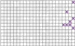
In this section we show how the techniques established in the paper can be used to predict house prices. This can be of interest in real estate and urban economics, as well as for property developers. Indeed, spatial methods are frequently used in these fields, as studied for instance by Iversen Jr (2001), Banerjee et al. (2004) and Majumdar et al. (2006). We use median house price data for census blocks in California from the 1990 census from Pace and Barry (1997), available at www.spatial-statistics.com. We confine our analysis to the city of Los Angeles. The data is gridded as follows: a grid of square cells is superimposed on Los Angeles, from N to N and W to W. The grid covers a total of 5259 observations. The average of the median house values for each cell is calculated and the 322 such observations form our sample. The gridding is shown in Figure 2, in which the 8 empty cells are filled and marked with a cross. We wish to predict the house price for these cells. House price data is not a zero mean process, so we subtract the sample mean using the whole sample from each cell.
We proceed in the following way: to obtain the coefficients , and in and (4.6) we use the sublattice formed of the first 19 columns of cells. This sublattice contains no missing observations. Once the coefficients are obtained we construct predictions using the remaining sublattice, in a step-by-step manner. The shaded-and-crossed cell (8,20) is predicted first, followed by (8,21) and (8,22). We then predict (4,21), followed by (7,22), (9,23), (6,23) and (1,23).
The predicted values are tabulated for various values of and in Tables 5 and 6. The predicted values are quite stable across the choices using either the periodogram or AR spectral estimate. They most closely match those obtained when in (4.6). In the latter case we compare in Table 7 the order selection criteria proposed by Gupta (2018), which include the usual FPE and BIC (denoted with a ) as well as corrected version that account for the spatial case (denoted with and ). The FPE tends to favour longer lag lengths no matter which version is used, as do and . However the latter as well as are not monotonically decreasing in lag length, unlike , and . Thus the latter three are likely to overfit and seem undesirable. If we impose a selection rule that picks the desirable lag order as the first instance when the selection criteria shows an increase with lag length, then we get using and . indicates a choice of , on the other hand. All considered, it seems that is a reasonable choice.
| (8,20) | (8,21) | (8,22) | (4,21) | (7,22) | (9,23) | (6,23) | (1,23) | |||
|---|---|---|---|---|---|---|---|---|---|---|
| (1,1) | 0.5645 | 0.5540 | 0.5384 | 0.6976 | 0.6671 | 0.1962 | 0.9337 | 0.4518 | ||
| 0.5244 | 0.5529 | 0.5523 | 0.6643 | 0.6256 | 0.1969 | 0.8770 | 0.4348 | |||
| (1,2) | 0.8054 | 0.5312 | 0.8791 | 1.2740 | 0.8797 | 1.0049 | 1.2029 | 0.6338 | ||
| 0.7043 | 0.4290 | 0.7684 | 1.1141 | 0.7693 | 0.8788 | 1.0520 | 0.5543 | |||
| (2,1) | 1.0691 | 0.8761 | 0.3926 | 1.4462 | 1.9503 | 0.7717 | 0.8519 | 1.0789 | ||
| 0.9828 | 0.8133 | 0.4722 | 1.3612 | 1.7429 | 0.6726 | 0.8448 | 1.0044 | |||
| (2,2) | 2.0717 | 1.7439 | 1.4680 | 3.0421 | 2.4033 | 2.3360 | 2.3242 | 2.0935 | ||
| 1.8934 | 1.4566 | 1.1207 | 2.7803 | 2.1965 | 2.1349 | 2.1242 | 1.9134 | |||
| (2,3) | 1.9970 | 1.6205 | 1.3149 | 2.9325 | 2.3167 | 2.2518 | 2.2404 | 2.0181 | ||
| 1.7926 | 1.3057 | 0.9511 | 2.6323 | 2.0796 | 2.0213 | 2.0111 | 1.8115 | |||
| (1,3) | 0.8150 | 0.5414 | 0.8899 | 1.2892 | 0.8902 | 1.0169 | 1.2173 | 0.6414 | ||
| 0.7218 | 0.4460 | 0.7874 | 1.1419 | 0.7885 | 0.9007 | 1.0782 | 0.5681 |
| (8,20) | (8,21) | (8,22) | (4,21) | (7,22) | (9,23) | (6,23) | (1,23) | |||
|---|---|---|---|---|---|---|---|---|---|---|
| (1,1) | 1.6525 | 1.2876 | 1.0325 | 2.4728 | 1.6663 | 2.1204 | 1.6825 | 1.7266 | ||
| (1,2) | 1.5373 | 1.2516 | 0.8473 | 2.3741 | 1.7944 | 1.8452 | 1.7626 | 1.5659 | ||
| (2,1) | 1.8138 | 1.6433 | 1.1237 | 2.4881 | 1.8545 | 2.3404 | 1.7547 | 2.3233 | ||
| (2,2) | 1.8703 | 1.9858 | 1.4089 | 2.6079 | 2.4100 | 2.4992 | 2.0862 | 2.2252 | ||
| (3,2) | 1.7925 | 1.9298 | 1.4400 | 2.4489 | 2.6472 | 2.5962 | 2.4021 | 1.9518 | ||
| (4,3) | 2.4465 | 2.2325 | 1.9075 | 2.0319 | 3.1207 | 3.5439 | 2.8234 | 2.0841 |
| (1,1) | 0.5979 | 0.6001 | 0.5990 | 0.5472 | 0.5639 | 0.5555 | ||||
| (1,2) | 0.5973 | 0.5979 | 0.5976 | 0.5144 | 0.5183 | 0.5164 | ||||
| (2,1) | 0.5953 | 0.6042 | 0.5997 | 0.4766 | 0.5377 | 0.5062 | ||||
| (2,2) | 0.5946 | 0.6008 | 0.5977 | 0.4351 | 0.4728 | 0.4535 | ||||
| (3,2) | 0.5943 | 0.6105 | 0.6024 | 0.4022 | 0.5018 | 0.4489 | ||||
| (4,3) | 0.5824 | 0.6081 | 0.5953 | 0.2129 | 0.3058 | 0.2543 |
6 Conclusion
In this paper we have dealt with the problem of prediction when the data is collected on a lattice. To do so, we considered unilateral representations of and in particular the canonical factorization of the spectral density function, the latter being possible as observed by Whittle (1954). Our approach does not need any parameterization of the model (i.e. the covariogram structure of the data), so we avoid the consequences that a wrong parameterization can have in the predictor. We have also compared our methodology to one based on the space domain by using a finite approximation of the unilateral autoregressive model in .
However, it might be interesting to examine how our proposed methodology compares with one based on the conditional autoregressive () representation of Besag (1974). That is, let be given by
| (6.1) | |||||
Note that our definition in implies that is, among other characteristics, homogeneous. The representation of given in suggests to predict a value at a location , and , by
| (6.2) |
where and are respectively the least squares estimator of and , and with the convention that if it were not observed. This is in the same spirit as we did with our predictor in . On the other hand, if we were interesting to predict a value at a location , we might then use
| (6.3) |
However to compute the prediction we would also need to replace the unobserved by its prediction as in . The latter might be done in an iterative fashion similar to what we did in .
.
Mathematical Appendix
Appendix A Proofs of Theorems
For the sake of notational simplicity, we shall assume that and also that , so that and say. Also to simplify the notation we shall write instead of given in . That is,
| (A.1) |
A.1 Proof of Theorem 1
We shall examine part , since part follows by Lemma 2 and standard arguments. By the Cramér-Wold device, it suffices to show that for a finite set of constants , ,
| (A.2) |
First, by definition of and , we have that
| (A.3) |
Because standard inequalities and then Lemma 3 yield that
| (A.4) |
the left side of is, by Lemma 3,
| (A.5) | |||||
after using Taylor series expansion of around and Condition . Now, the absolute value of the second term on the right of the last displayed expression is bounded by
| (A.6) |
by Lemmas 2 and 3. So, we conclude that
where is a step function defined as
when and , . Now, using Lemma 1, we have that for all ,
So, we conclude that the left side of is
after we observe that Condition implies that
Recall that . From here the conclusion is standard proceeding as in the proof of Theorems 1 and 2 of Hidalgo (2009), see also Robinson and Vidal-Sanz , and so it is omitted.
A.2 Proof of Theorem 2
Define , and . We begin with part . First by definition,
| (A.7) |
which by Taylor expansion of , in Lemma 2 and Condition , it is
Now using the inequality
| (A.8) |
we have that
Thus using that , the right side of is
where in the second equality we have used and and then Condition and for the third equality that
and then that since , given in , is twice continuously differentiable so that . From here we conclude the proof of part by standard algebra.
Next, we show part . By Cramér-Wold device, it suffices to examine that for any set of finite constants , the behaviour of
First, by definitions of and , we have that
proceeding as in the proof of Theorem 1, where and were defined there. So, because for , denoting , we conclude that
proceeding as in the proof of Theorem 1, where and
by Lemma 4. From here the conclusion of the theorem follows by standard delta arguments.
A.3 Proof of Theorem 3
We begin with part . To that end, it suffices to show that
| (A.11) |
By definition of and Taylor expansion of , a typical component on the left of is
| (A.12) |
Now implies that
by Theorem of Serfling (1980), p. 14 because Condition implies that is uniformly integrable and Theorem 2 and the continuous mapping theorem implies that . So, using we conclude that is
where in the first equality we use and in the second equality that Lemma 6 implies that
because and is a summable sequence.
So, we conclude that the left side of is
where .
We now conclude because using that , , a typical component of is times
where we have taken . From here the conclusion is standard since is summable.
Part follows by similar arguments to those in and Lemma 2, so it is omitted.
A.4 Proof of Theorem 4
We begin with part. For that purpose, denote
where . Then,
| (A.14) |
The second moment of is clearly since for any and for any and that . Next, the second moment of the last term on the right of is bounded by
by Lemma 7 and that the covariance of is summable. Thus, it remains to examine the behaviour of on the right of , which is
| (A.15) | |||
Now Theorem 3 part and summability of the covariance of yields that the second moment of the second term of is . So, to complete the proof of part , we need to look at the first term, which is
because using expression , . Finally
by triangle and Cauchy-Schwarz inequalities and then Condition . Similarly we have that , which concludes the proof of part .
We now show part , that is when . For that purpose, it is convenient to recall our representation in . The reason is because the prediction error can be written as
where is similar to but where
and as defined in . Now, it is obvious that we have the same type of (statistical) results for as those obtained for , and hence proceeding as in part , we conclude that
and that
This concludes the proof of the theorem.
Appendix B Technical Lemmas
To simplify the notation, we abbreviate by in what follows.
Lemma 1.
Under Conditions we have that
where is a triangular array sequence of r.v.’s such that .
Proof.
The proof follows easily from Lemma 4 of Hidalgo (2009), and so it is omitted.
Lemma 2.
Assuming , and .
Proof.
We begin with part . By definition of and then Taylor series expansion of , we have that
So, it suffices to examine the behaviour of . By definition and ,
| (B.1) | |||||
because is a four times differentiable function and if is an odd integer. From here the conclusion follows by standard arguments, because is a continuous differentiable function, so that the Riemman sums converge to their integral counterpart.
Part follows using Lemma 6.
Lemma 3.
Assuming, , for all
Proof.
Because , the left side of the last displayed equality is, up to multiplicative constants, bounded by
The first term of the last displayed expression is by Lemma 1, whereas the second term follows by standard arguments, as is an sequence of r.v.’s with finite fourth moments.
Lemma 4.
Proof.
First,
where for notational simplicity, we assume that .
Next, because , we have then that is
| (B.3) | |||||
Let’s examine a typical term on the right of , say
By definition, the last displayed expression is
Because , it easy to see that the first term is , whereas the second term is
so is the third term by symmetry. Finally the fourth term is different than zero if , in which case becomes
Then, proceeding similarly with the other three terms in , we can conclude, except negligible terms, that it is
From here we conclude by Lemma 4 of Hidalgo and Yajima (2002).
Lemma 5.
Under Condition , we have that
Proof.
The proof is standard because four times continuous differentiability of implies that for .
The next lemma is regarding the approximation of integrals by sums. Taking for simplicity that and recalling our notation, we have then that . Also, use the standard notation, , , and for a function
Lemma 6.
Assume that is a function times continuously differentiable in . Then,
| (B.4) |
where is a sequence such that and , ,…, are finite constants.
Proof.
The left side of is
by Taylor’s expansion and where denotes a point between and . Now, the right side of is
| (B.6) |
Denoting and , , and proceeding as with , we conclude that , and hence the left side of , is
after observing that , , are respectively continuous differentiable functions.
Lemma 7.
Under Condition , for all ,
where is a summable sequence.
Proof.
By definition, is
| (B.7) |
where . Because is four times continuous differentiable, the third term of is
| (B.8) |
by Lemma 6. This is the case after we notice that there is given by
which is clearly summable since , and because and for every implies that
Next, the second term of is bounded in absolute value by
| (B.9) | |||||
by Lemma 5 and that , where denotes the summation in
Finally, by definition of and , the first term of is
| (B.10) |
where using the inequality in , we have that is
| (B.11) | |||||
by Lemma 6 and where now , . Next, because is four times continuously differentiable, it implies that and thus by standard arguments, the right side of is
From here and using Taylor expansion of , we obtain that is
| (B.12) | |||||
where , , are the Fourier coefficients of , which are summable because is times differentiable function. The conclusion of the lemma now follows by gathering terms , and .
References
- Baltagi et al. (2007) Baltagi, B. H., H. H. Kelejian, and I. R. Prucha (2007). Analysis of spatially dependent data. Journal of Econometrics: Annals Issue.
- Banerjee et al. (2004) Banerjee, S., A. E. Gelfand, J. R. Knight, and C. F. Sirmans (2004). Spatial modeling of house prices using normalized distance-weighted sums of stationary processes. Journal of Business & Economic Statistics 22, 206–213.
- Batchelor and Reed (1918) Batchelor, L. and H. Reed (1918). Relation of the variability of yields of fruit trees to the accuracy of field trials. Journal of Agricultural Research XII, 245–283.
- Besag (1974) Besag, J. (1974). Spatial interaction and the statistical analysis of lattice systems. Journal of the Royal Statistical Society Series B 36, 192–236.
- Bester et al. (2011) Bester, C. A., T. G. Conley, and C. B. Hansen (2011). Inference with dependent data using cluster covariance estimators. Journal of Econometrics 165, 137–151.
- Bester et al. (2016) Bester, C. A., T. G. Conley, C. B. Hansen, and T. J. Vogelsang (2016). Fixed-b asymptotics for spatially dependent robust nonparametric covariance matrix estimators. Econometric Theory 32, 154–186.
- Bhansali (1974) Bhansali, R. J. (1974). Asymptotic properties of the Wiener-Kolmogorov predictor. I. Journal of the Royal Statistical Society. Series B 36, 61–73.
- Bhansali (1978) Bhansali, R. J. (1978). Linear prediction by autoregressive model fitting in the time domain. Annals of Statistics 60, 224–231.
- Breidt et al. (2001) Breidt, F. J., R. A. Davis, and A. A. Trindade (2001). Least absolute deviation estimation for all-pass time series models. Annals of Statistics 29, 919–946.
- Brillinger (1981) Brillinger, D. R. (1981). Time Series: Data Analysis and Theory. Holden Day, San Francisco.
- Cavaliere et al. (2020) Cavaliere, G., H. B. Nielsen, and A. Rahbek (2020). Bootstrapping noncausal autoregressions: with applications to explosive bubble modeling. Journal of Business & Economic Statistics 38, 55–67.
- Conley (1999) Conley, T. G. . (1999). GMM estimation with cross sectional dependence. Journal of Econometrics 92, 1–45.
- Conley and Molinari (2007) Conley, T. G. and F. Molinari (2007). Spatial correlation robust inference with imperfect distance information. Journal of Econometrics 140, 76–96.
- Cressie and Huang (1999) Cressie, N. and H. Huang (1999). Classes of nonseparable, spatio-temporal stationary covariance functions. Journal of the American Statistical Association 94, 1330–1340.
- Cressie (1993) Cressie, N. A. (1993). Statistics for Spatial Data. Wiley Series in Probability and Mathematical Statistics: Applied Probability and Statistics. John Wiley & Sons.
- Dahlhaus and Künsch (1987) Dahlhaus, R. and H. Künsch (1987). Edge effects and efficient parameter estimation for stationary random fields. Biometrika 74, 877–882.
- Davis et al. (2013) Davis, R. A., C. Klüppelberg, and C. Steinkohl (2013). Statistical inference for max-stable processes in space and time. Journal of the Royal Statistical Society Series B 75, 791–819.
- Fernandez-Casal et al. (2003) Fernandez-Casal, R., W. Gonzalez-Manteiga, and M. Febrero-Bande (2003). Flexible spatio-temporal stationary variogram models. Statistics and Computing 13, 127–136.
- Gao et al. (2006) Gao, J., Z. Lu, and D. Tjøstheim (2006). Estimation in semiparametric spatial regression. The Annals of Statistics 34, 1395–1435.
- Genton and Koul (2008) Genton, M. G. and H. L. Koul (2008). Minimum distance inference in unilateral autoregressive lattice processes. Statistica Sinica 18, 617–631.
- Gupta (2018) Gupta, A. (2018). Autoregressive spatial spectral estimates. Journal of Econometrics 203, 80–95.
- Guyon (1982) Guyon, X. (1982). Parameter estimation for a stationary process on a -dimensional lattice. Biometrika 69, 95–105.
- Haining (1978) Haining, R. P. (1978). The moving average model for spatial interaction. Transactions of the Institute of British Geographers 3, 202–225.
- Helson and Lowdenslager (1958) Helson, H. and D. Lowdenslager (1958). Prediction theory and Fourier series in several variables. Acta Mathematica 99, 165–202.
- Helson and Lowdenslager (1961) Helson, H. and D. Lowdenslager (1961). Prediction theory and Fourier series in several variables. II. Acta Mathematica 106, 175–213.
- Hidalgo (2009) Hidalgo, J. (2009). Goodness of fit for lattice processes. Journal of Econometrics 151, 113–128.
- Hidalgo and Yajima (2002) Hidalgo, J. and Y. Yajima (2002). Prediction and signal extraction of strongly dependent processes in the frequency domain. Econometric Theory 18, 584–624.
- Iversen Jr (2001) Iversen Jr, E. (2001). Spatially disaggregated real estate indices. Journal of Business & Economic Statistics 19, 341–357.
- Jenish (2016) Jenish, N. (2016). Spatial semiparametric model with endogenous regressors. Econometric Theory 32, 714–739.
- Jenish and Prucha (2012) Jenish, N. and I. R. Prucha (2012). On spatial processes and asymptotic inference under near-epoch dependence. Journal of Econometrics 170, 178 – 190.
- Korezlioglu and Loubaton (1986) Korezlioglu, H. and P. Loubaton (1986). Spectral factorization of wide sense stationary processes on . Journal of Multivariate Analysis 19, 24–47.
- Lanne and Saikkonen (2013) Lanne, M. and P. Saikkonen (2013). Noncausal vector autoregression. Econometric Theory 29, 447–481.
- Lanne and Saikonnen (2011) Lanne, M. and P. Saikonnen (2011). Noncausal autoregressions for economic time series. Journal of Time Series Econometrics 3, 1–30.
- Lewis and Reinsel (1985) Lewis, R. and G. C. Reinsel (1985). Prediction of multivariate time series by autoregressive model fitting. Journal of Multivariate Analysis 16, 393–411.
- Limaye and Zeltser (2009) Limaye, B. V. and M. Zeltser (2009). On the Pringsheim convergence of double series. Proceedings of the Estonian Academy of Sciences 58, 108.
- Majumdar et al. (2006) Majumdar, A., H. J. Munneke, A. E. Gelfand, S. Banerjee, and C. F. Sirmans (2006). Gradients in spatial response surfaces with application to urban land values. Journal of Business & Economic Statistics 24, 77–90.
- McElroy and Holan (2014) McElroy, T. S. and S. H. Holan (2014). Asymptotic theory of cepstral random fields. The Annals of Statistics 42, 64–86.
- Mercer and Hall (1911) Mercer, W. B. and A. D. Hall (1911). The experimental errors of field trials. Journal of Agricultural Science IV, 107–132.
- Mitchell et al. (2005) Mitchell, M. W., M. G. Genton, and M. L. Gumpertz (2005). Testing for separability of space-time covariances. Environmetrics 16, 819–831.
- Nychka et al. (2015) Nychka, D., S. Bandyopadhyay, D. Hammerling, F. Lindgren, and S. Sain (2015). A multiresolution Gaussian process model for the analysis of large spatial datasets. Journal of Computational and Graphical Statistics 24, 579–599.
- Pace and Barry (1997) Pace, R. K. and R. Barry (1997). Sparse spatial autoregressions. Statistics & Probability Letters 33, 291 – 297.
- Robinson (2007) Robinson, P. M. (2007). Nonparametric spectrum estimation for spatial data. Journal of Statistical Planning and Inference 137, 1024–1034.
- Robinson (2011) Robinson, P. M. (2011). Asymptotic theory for nonparametric regression with spatial data. Journal of Econometrics 165, 5–19.
- Robinson and Vidal Sanz (2006) Robinson, P. M. and J. Vidal Sanz (2006). Modified Whittle estimation of multilateral models on a lattice. Journal of Multivariate Analysis 97, 1090–1120.
- Roknossadati and Zarepour (2010) Roknossadati, S. M. and M. Zarepour (2010). -estimation for a spatial unilateral autoregressive model with infinite variance innovations. Econometric Theory 26, 1663–1682.
- Serfling (1980) Serfling, R. (1980). Approximation Theorems of Mathematical Statistics. John Wiley & Sons.
- Solo (1986) Solo, V. (1986). Modeling of two-dimensional random fields by parametric Cepstrum. IEEE, Transactions on Information Theory 42, 743–750.
- Stein (1999) Stein, M. (1999). Interpolation of Spatial Data: Some Theory for Kriging. Spinger-Verlag, New York.
- Wang et al. (2013) Wang, H., E. M. Iglesias, and J. M. Wooldridge (2013). Partial maximum likelihood estimation of spatial probit models. Journal of Econometrics 172, 77–89.
- Whittle (1954) Whittle, P. (1954). On stationary processes in the plane. Biometrika 41, 434–449.