Using Multiple Imputation to Classify Potential Outcomes Subgroups

Abstract

With medical tests becoming increasingly available, concerns about over-testing, over-treatment and health care cost dramatically increase. Hence, it is important to understand the influence of testing on treatment selection in general practice. Most statistical methods focus on average effects of testing on treatment decisions. However, this may be ill-advised, particularly for patient subgroups that tend not to benefit from such tests. Furthermore, missing data are common, representing large and often unaddressed threats to the validity of most statistical methods. Finally, it is often desirable to conduct analyses that can be interpreted causally. Using the Rubin Causal Model framework, we propose to classify patients into four potential outcomes subgroups, defined by whether or not a patient’s treatment selection is changed by the test result and by the direction of how the test result changes treatment selection. This subgroup classification naturally captures the differential influence of medical testing on treatment selections for different patients, which can suggest targets to improve the utilization of medical tests. We can then examine patient characteristics associated with patient potential outcomes subgroup memberships. We used multiple imputation methods to simultaneously impute the missing potential outcomes as well as regular missing values. This approach can also provide estimates of many traditional causal quantities of interest. We find that explicitly incorporating causal inference assumptions into the multiple imputation process can improve the precision for some causal estimates of interest. We also find that bias can occur when the potential outcomes conditional independence assumption is violated; sensitivity analyses are proposed to assess the impact of this violation. We applied the proposed methods to examine the influence of 21-gene assay, the most commonly used genomic test in the United States, on chemotherapy selection among breast cancer patients.

1 Introduction

Newly diagnosed cancer patients and their physicians frequently face the challenges of deciding which tests and subsequent treatments to use. The testing itself can be both invasive and expensive, and the cost of medical tests reaches 70 billion dollars annually Brill . Furthermore, test results do not predictably inform treatment decisions, either because guidelines are not always available or they are not followed in practice. Thus, describing how testing impacts the choice of treatment in general practice is of fundamental importance. We will view this problem in a causal framework, in which taking the test is the exposure of interest, and the treatment received is the outcome of interest.

An example is the use of the 21-gene recurrence score (RS) assay in breast cancer care, the most commonly used genomic assay in the United States. The test is used to inform recommendations about the use of chemotherapy. Women who get a high score on the test are recommended to take chemotherapy to reduce their risk of recurrence, whereas women with a low score are not because they have a good prognosis and are expected to receive little additional benefit from chemotherapy. Prior studies have demonstrated that RS tests can provide more precise estimation of the risk of cancer recurrence and the need for chemotherapy than do traditional histopathologic features (e.g., tumor grade and size) Albain ; Schnipper ; Paik1 ; Habel ; Paik2 ; Dowsett ; Goldstein . Even though the current clinical guidelines only endorse the use of RS assay in selected patients with certain clinical characteristics Harris ; NCCN , more and more patients who do not meet these criteria are being selected for RS testing. Also, chemotherapy is highly morbid, and many believe it is being over-prescribed Sparano ; Manj . Thus, there is a pressing need to measure the influence of the RS assay on chemotherapy decisions to evaluate whether the test is being used in an efficient manner and acted upon appropriately in general practice.

Determining the influence of testing on treatment selection in a community practice setting is not well studied and is challenging to quantify using standard methods. First, selection bias may occur because testing is not offered randomly. Both clinical factors as well as patient and physician preferences influence whether testing is offered, and this confounds the effect of testing on treatment selection Bosco ; Salas . Second, while causal inference methods such as propensity-score based methods can address selection bias and give effect estimates with desirable causal interpretations, they are limited to estimating an overall effect of testing on treatment selection, not how testing changes treatment plans within patient subgroups. The overall effect can obscure the degree to which treatment plans are changed by testing. For example, the overall effect can be zero, if testing encourages and discourages treatment for an equal number of patients, even though testing did change treatment plans. Third, missing data are common, especially when multiple data sources are combined as in many studies. Missing data are often-unaddressed threats to the validity of statistical methods.

In this paper, we propose to use a potential outcomes framework (i.e., a causal inference framework) Holland to measure the influence of testing by comparing treatment use when everyone is tested with when no one is tested. This minimizes selection bias affecting test use that is attributable to observed confounders. Specifically, we propose to classify patients into four potential outcomes subgroups defined by their expected treatment decisions with a given test versus without the test: 1) Never-Treated: those who would not have been treated with or without the test; 2) Treatment-Encouraged: those who would have been treated with the test but would not have been treated without the test; 3) Treatment-Discouraged: those who would not have been treated with the test but would have been treated without the test; 4) Always-Treated: those who would have been treated with or without the test. These four subgroups (listed in Table 1) are called potential outcomes subgroups Holland . A patient’s membership in these subgroups may be driven by patient characteristics or by systemic factors (e.g., treating physician). Such classification can also suggest ways to improve the utilization of medical tests in treatment decisions. The classification recognizes that a medical test can have different influences on treatment decisions for different patients; i.e., there may be effect heterogeneity of testing on treatment. With the classification, we will be able to measure how many patients’ treatment selections are changed (or unchanged) by test results for overall and key clinical subgroups, and also quantify how much test results encourage (or discourage) treatment selections. The potential outcomes subgroups bear some resemblance to principal stratification Frangakis , which has been extensively used by us and others to study the causal effect of intermediate variables (e.g., degree of compliance, surrogate markers) Huang ; Li ; Roy . However, unlike principal strata, which are defined by the joint distribution of intermediate variables under different exposure status, here we focus on the joint distribution of the outcome of interest (here treatment received) under different exposure status (here test received). We believe this framework provides important conceptual and practical advances in studying the influence of medical testing in treatment selection. We will also demonstrate its advantages of providing unique and highly relevant causal quantities of interest over alternative causal inference methods.

We will classify patients into these potential outcomes subgroups by exploring the close connection between missing data analysis and causal inference. Since two potential outcomes of the same patients are not simultaneously observed, we will use multiple imputation methods to impute the unobserved potential outcomes to enable us to make causal inferences. Multiple imputation methods have been used to impute missing potential outcomes in solving different problems in causal inference literature Rubin ; Taylor ; Gutman ; Bondarenko ; Westreich ; Miao ; Zhou . These methods have the advantage of simultaneously handling standard missing data in observable variables (e.g. due to non-response) and missing potential outcomes. However, since missing data analysis and causal inference have different objectives and data structures, there are important distinctions between them. First, causal inference focuses on comparing the potential outcomes of the same patient under different exposure levels; while missing data analyses do not. Second, the causal assumptions (e.g., ignorability of treatment assignment or potential outcomes conditional independence) are not usually made in standard missing data analyses. Third, causal inference distinguishes pre-exposure variables from post-exposure variables and usually does not use a post-exposure variable, while missing data analyses do not differentiate them and often utilize a post-exposure variable in the imputation models if it is predictive of other variables with missing values. Fourth, the missing potential outcomes problem is highly structured such that only one of two potential outcomes is observed for any patient when the exposure variable is binary. In this situation, the missing data indicator is identical to the binary exposure variable. Fifth, since no two potential outcomes of the same patient can be observed simultaneously, there is no information about the correlation between two potential outcomes of the same patient. This distinct data structure is similar to the missing data structure in the literature on ”statistical matching” Kim ; Conti . More detailed discussions about missing data analyses and causal inference can be found by Ding and Li (2018) and Westreich et al (2015) Ding ; Westreich . In this paper, we will study the performance of our proposed methods. We will also examine the efficiency gain of our causal estimates when we incorporate the knowledge of our data structure and causal inference assumptions into the multiple imputation process. We will propose sensitivity analyses to investigate the violation of one of the key causal inference assumptions on causal estimates (i.e., potential outcomes conditional independence). Additionally, we will explore the impact of incorporating a post-exposure variable in the multiple imputation process on the causal estimates. Furthermore, we will demonstrate that this approach is more robust towards certain types of model mis-specification than other causal methods (e.g., propensity-score based methods).

Table 1: Potential outcomes subgroups defined by the effect of testing on treatment selection.

	Treatment Selection with Test ($Y_{1}$)
Treatment Selection
without Test ($Y_{0}$)	Yes	No
Yes	Always Treated	Treatment Discouraged
No	Treatment Encouraged	Never Treated

To illustrate our methods, we will examine the impact of the RS assay on the decision to undergo chemotherapy for breast cancer patients. The analyses will use combined data sets from the Surveillance, Epidemiology, and End Results databases (SEER) registry, genomic testing laboratories, and patient/physician surveys, recently collected from the ICanCare Study Friese ; LiY . The data linkage was a unique survey-registry-industry collaboration and the ICanCare study was part of the only program project funded by National Cancer Institute that focused on cancer treatment decision making.

2 Notation, the Causal Framework and Quantities of Interest

Let $Y$ represent the treatment receipt (i.e., the outcome of interest, 0/1 for no/yes), $Z$ the status of being tested (i.e., the exposure of interest, 0/1 for no/yes), $X$ a set of covariates and $R$ the test result. Naturally, $R$ only exists for testers and is a post-exposure variable. We assume some observations are missing in $Y$, $R$ and in some variables of $X$. Let $M$ be the associated missing-data indicator matrix for these observable variables. The observed and missing parts of $Y$ are denoted by $Y^{obs}$ and $Y^{mis}$ respectively, and the same for $X$.

For each patient, we assume there are two potential outcomes, $Y_{1}$ and $Y_{0}$, corresponding to being tested or not ($Z=1,0$). Let $Y_{1}$ indicate a patient’s treatment status that would be observed if the patient is tested and $Y_{0}$ otherwise. If we know both $Y_{1}$ and $Y_{0}$ for every patient, we can infer whether a test causes a change in treatment selection by comparing $Y_{1}$ to $Y_{0}$, and calculate many causal quantities that are free of selection bias. In this manuscript, we choose several representative causal quantities including: (1) average testing effect (ATE), E($Y_{1}-Y_{0}$), for the overall population and patient subgroups; (2) marginal odds ratio (MOR), $[P_{1}(1-P_{0})]/[P_{0}(1-P_{1})]$ where $P_{0}=P(Y_{0}=1)$ and $P_{1}=P(Y_{1}=1)$; and (3) the fractions of patients in each of the four potential outcome subgroups: ($Y_{0}=0$, $Y_{1}=0$) for the never-treated, ($Y_{0}=0$, $Y_{1}=1$) for the treatment-encouraged, ($Y_{0}=1$, $Y_{1}=0$) for the treatment-discouraged, and ($Y_{0}=1$, $Y_{1}=1$) for the always-treated group, which are denoted by $P(00)$, $P(01)$, $P(10)$ and $P(11)$ respectively. The MOR defined in (2) compares the odds of treatment use if everyone were tested to the odds if no one were tested. Odds ratios in observational studies are usually association measures and lack causal interpretations because of confounding. In contrast, MORs do have causal interpretations. Based on the fractions defined in (3), we can calculate many quantities that are functions of them. For example, we can calculate the proportion of patients whose treatment plans are changed by the use of testing (i.e., the proportion of patients who were either treatment encouraged or discouraged), $P(01)+P(10)$, and the proportion of patients whose treatment plans are not changed (i.e., the proportion of patients who were either never-treated or always-treated), $P(00)+P(11)$. In fact, ATE is also a function of these fractions, which is equal to the difference in the proportions in the “treatment encouraged” and “treatment discouraged” subgroups, i.e., $P(01)-P(10)$. We are also interested in estimating the associations between patient characteristics and patient membership in these potential outcomes subgroups.

3 Estimating the Distributions of Potential Treatment Selection

To measure the causal influence of a test, ideally, we wish to know the treatment plan for each patient when she is tested and when she is not. That is, we wish to know both $Y_{0}$ and $Y_{1}$. However, the treatment plan is observable for a given patient in only one of these two scenarios because she may not get tested and; even if she does, her pre-test treatment plan is not usually documented. Formally, this is a missing data problem. We use sequential regression multiple imputation (or sometimes called the fully conditional specification method) Raghu ; Van to impute the unobserved (counterfactual) treatment plan for each patient, which we term the potential outcomes multiple imputation method (POMI). That is, for patients who received the test, we impute what would have been their treatment plans had they not received the test. And for patients who did not receive the test, we impute what would have been their treatment plans had they received the test from the predictive distribution of $Y$ given $X$ and/or $R$. Once we have complete information for $Y_{0}$ and $Y_{1}$ after imputation, we can calculate the causal quantities of interest. Since we have incomplete information in observable variables $Y$, $X$ and $R$, we can simultaneously impute missing potential outcomes and missing values in these observable variables during the multiple imputation process using the same imputation methods.

Although we can view causal inference as a missing data problem, there are distinct features of causal inference different from standard missing data problems. As stated in the Introduction section, the objectives of causal inference are to obtain the causal effect of an exposure on the outcome, while missing data analyses are to handle missing values in variables, utilize incomplete information and reduce bias due to non-response. Hence, some assumptions are closely related but others are different. Below we list four assumptions used in missing data and/or causal inference literature:

1. Missing at random Little , $f(M|Z,Y,X,R)=f(M|Z,Y^{obs},X^{obs},R^{obs})$. That is, missingness can be explained by the observed data. This is a standard assumption in the missing data literature. Note that $f()$ denotes a probability density or mass function for the distribution of either a continuous or discrete variable in this manuscript.

2. Stable unit treatment value assumption (SUTVA) Rubin ; Rubin1 . The potential outcomes of one patient are unaffected by the potential outcomes or testing status of other patients. This is a standard assumption in the causal inference literature. This assumption is not usually explicitly made, but it is implied in the missing data literature.

3. Ignorability of exposure Rubin2 , $(Y_{0},Y_{1})\bot Z|X$. This assumption means that the receipt of test is “randomized” for subjects with the same set of covariates $X$, that is, there are no unmeasured confounders between $Z$ and $Y$ after adjustment for $X$. It is a standard assumption in the causal inference literature, and a special case of the missing-at-random assumption (see Assumption 1).

4. Potential outcomes conditional independence, $(Y_{0}\bot Y_{1})|X$. This assumption states that two potential outcomes are conditionally independent. However, since the two potential outcomes are never observed together, we have no information about the correlation, independence or joint distribution of $Y_{0}$ and $Y_{1}$ from the observed data. This assumption is frequently made in the causal inference literature Zhang ; Efron ; Daniels . It is also made in the missing data and survey methodology literature when applying the less-known statistical matching technique to conduct a joint analysis on variables that are never jointly observed Kim ; Conti . We will explore robustness of our methods to this conditional independence assumption using sensitivity analyses.

These assumptions will be essential to facilitating identification and estimation of causal quantities of interest.

We propose to impute the missing values in $X$ and $R$ as well as the missing potential outcomes ($Y_{0}$ and $Y_{1}$) iteratively variable-by-variable using a sequence of conditional regression models until convergence: $f(X_{j}|X_{(-j)},Z,Y_{0},Y_{1},R)$, $f(R|X,Z,Y_{0},Y_{1})$, $f(Y_{0}|Y_{1},Z,X,R)$, $f(Y_{1}|Y_{0},Z,X,R)$ for any $j$ Kenn ; Van ; Raghu . Note that $X=(X_{1},\cdots,X_{k})$ and $X_{(-j)}=(X_{1},\cdots,X_{(j-1)},X_{(j+1)},\cdots,X_{k})$ denoting the collection of the $k-1$ variables in $X$ except $X_{j}$. This method is the sequential regression multiple imputation method and has its advantages in handling non-normal data Raghu . We can evaluate how well the missing variables are imputed as in regular missing data imputation problems.

We impute the missing values $D$ times to give a range for each imputed value to reflect prediction uncertainty. We then obtain the estimates of the quantities of interest for each of the $D$ imputed data sets before combining these estimates and their variances across $D$ imputed data sets using Rubin’s formula Rubin2 . Let $\Delta$ represent any quantity of interest, $\widehat{\Delta}_{d}$ the point estimate and $W_{d}$ the within-imputation variance estimate of $\widehat{\Delta}_{d}$ for the $d$th imputed data set. The POMI estimate of $\Delta$ is obtained by averaging across $D$ imputed data sets, such that $\overline{\Delta}=\frac{1}{D}\sum_{d=1}^{D}\widehat{\Delta}_{d}$ where $d=1,\cdots,D$. The MI estimate of the variance of $\overline{\Delta}$ is $V=\overline{W}+(1+\frac{1}{D})B$, where $\overline{W}=\sum_{d=1}^{D}W_{d}/D$, $B=\sum_{d=1}^{D}(\widehat{\Delta}_{d}-\overline{\Delta})^{2}/(D-1)$. Note that $\overline{W}$ represents the average within-imputation variance and $B$ represents the between-imputation variance. The estimated $\Delta$ follows a $t$ distribution, with the degree of freedom $(D-1)[1+\frac{D}{D+1}(\overline{W}/B)^{2}]$ Schenker .

Specifically, the within-imputation variance for the estimated causal quantity of interest, ATE, for each imputed data set is calculated as follows: $\frac{1}{N-1}\left\{\left[\widehat{P}_{0}(1-\widehat{P}_{0})\right]+\left[\widehat{P}_{1}(1-\widehat{P}_{1})\right]-2(\widehat{P}_{11}-\widehat{P}_{0}\widehat{P}_{1})\right\}$, where $P_{11}=P(Y_{0}=1,Y_{1}=1)$ and $N$ is the sample size. The calculation of the within-imputation variance of the MOR estimate is more complicated than ATE because it is a non-linear function of $P_{0}$ and $P_{1}$. Since MOR is skewed and positive, we calculate the variance for the MOR estimate on a log scale. Specifically, for each imputed data set, we calculate the variance of $log(\widehat{MOR})$ using the delta method as follows: $\left[\widehat{P}_{0}+\widehat{P}_{1}-(\widehat{P}_{0}-\widehat{P}_{1})^{2}-2\widehat{P}_{11}\right]/\left[N\widehat{P}_{0}\widehat{P}_{1}(1-\widehat{P}_{0})(1-\widehat{P}_{1})\right]$. From the variance of $log(\widehat{MOR})$, we can then calculate the variance of the estimated MOR using the delta method again. The details for the variance calculation of estimated MOR are provided in the appendix. The within-imputation variances for estimated $P(00)$, $P(01)$, $P(11)$ and $P(10)$ are straightforward to calculate as multinomial proportions.

What we described so far are standard multiple imputation procedures. We will explore several features of causal inference that are distinct from standard missing data problems and see how the incorporation of them in the multiple imputation process impacts the causal estimates. These features will be incorporated through the four different POMI methods investigated in the following Simulation section. First, we will explicitly incorporate the causal inference assumptions (listed above as Assumptions 2, 3 and 4) and distinct data structures into the multiple imputations of missing potential outcomes. Under Assumption 2 and 3, we can simplify our imputation models for $Y_{0}$ and $Y_{1}$ such that $f(Y_{0}|Y_{1},Z,X,R)=f(Y_{0}|Y_{1},X,R)$ and $f(Y_{1}|Y_{0},Z,X,R)=f(Y_{1}|Y_{0},X,R)$. Under Assumptions 2, 3 and 4, we can further simplify our imputation models for $Y_{0}$ and $Y_{1}$ such that $f(Y_{0}|Y_{1},Z,X,R)=f(Y_{0}|X,R)$ and $f(Y_{1}|Y_{0},Z,X,R)=f(Y_{1}|X,R)$. Considering $R$ only exists for testers, we can further simplify the models such that $f(Y_{0}|Y_{1},Z,X,R)=f(Y_{0}|X)$. Second, we will explore the use of $Z$ in the multiple imputation process. $Z$ is a missing data indicator for $Y_{0}$ and $Y_{1}$. With an MAR assumption, multiple imputation does not need to include the missing data indicator Van . However, here $Z$ also serves the dual role as the exposure of interest. Third, we will investigate the use of test results $R$, a correlate of $Y$ and a post-exposure variable. In causal inference, post-exposure variables are not usually utilized because they may be in the causal pathway, and adjusting for them can bias results Robins . However, in standard missing data problems, post-exposure variables are usually included in the imputation models to increase the predictibility of variables with missing values, when post-exposure variables are correlated with the variables with missing values and hence contain additional information about them.

4 Simulations

We conduct simulations to examine: 1) the impact of $Z$, $R$ and causal inference assumptions on estimating the quantities of interest through comparisons of four POMI methods, which differ by whether the imputation models include $Z$, and/or $R$ or make certain causal inference assumptions; 2) the properties of causal estimates of ATE and MOR estimated by these four POMI methods and the inverse probability weighting method (IPW); 3) the properties of the unique causal estimates that are obtainable from the four POMI methods; 4) the robustness of the POMI methods towards model misspecification in comparisons with IPW; 5) sensitivity analyses towards the potential outcomes conditional independence assumption (Assumption 4); 6) the properties of the estimated association between patient characteristics and potential outcomes subgroup memberships through the POMI methods.

4.1 Simulation Design

We assume that $X$ includes two variables, $X_{1}$ and $X_{2}$. The distributions of $X_{1}$, $X_{2}$ and test results $R$ follow a multivariate normal distribution of

$$\left(\begin{array}[]{c}X_{1}\\ X_{2}\\ R^{*}\end{array}\right)\sim MVN\left(\left(\begin{array}[]{c}0\\ 1\\ -1\end{array}\right),\left(\begin{array}[]{ccc}1&0.3&0.3\\ 0.3&1&0.3\\ 0.3&0.3&1\end{array}\right)\right).$$ (10)

We further categorize $R^{*}$ into three groups to mimic the distribution of RS assay results in our data example. We let $R=1$ if $R^{*}<=-0.747$, $R=2$ if $-0.747<R^{*}<=0.282$ and $R=3$ if $R^{*}>0.282$. The distributions of $Z$, $Y_{0}$ and $Y_{1}$ are specified as follows: $\textit{logit}[P(Z=1)]=-1.5-X_{1}+0.5X_{2}+\alpha X_{1}X_{2}$, $\textit{logit}[P(Y_{0}=1)]=0.5X_{1}+X_{2}+\beta_{1}U$ and $\textit{logit}[P(Y_{1}=1)]=0.5X_{1}+X_{2}-1.5I(R_{1}=1)-0.5I(R_{1}=2)+I(R_{1}=3)+\beta_{2}U$. Note that $U$ is an unmeasured predictor of $Y$, which is used to induce a non-zero correlation between $Y_{0}$ and $Y_{1}$ after adjusting for $X$ and hence a violation of the potential outcomes conditional independence assumption. We assume $U\sim$ Normal(0,1). The default model parameter specifications in our simulations are: $\alpha=0$ (i.e., no interaction between $X_{1}$ and $X_{2}$), and $\beta_{1}=\beta_{2}=0$ (i.e., conditional independence between potential outcomes). However, we will let $\alpha\neq 0$ when conducting analyses to test the robustness of our methods towards model misspecifications. We will also allow $\beta_{1}$ and $\beta_{2}$ to be non-zero when conducting sensitivity analyses on the potential outcomes conditional independence assumption (Assumption 4).

Each simulated data set consists of $X_{1}$, $X_{2}$, $Z$, $R$ and $Y$. To be consistent with reality, the data set used in the data example does not have information on $U$, or on $R$ when $Z=0$. Further, we allow $X_{2}$ and $Y$ be partially missing. Let $M_{x}$ and $M_{y}$ be $0$ or $1$, indicating $X_{2}$ and $Y$ being available or missing, respectively. The models for the probability of missing $X_{2}$ and $Y$ are specified as follows: $\textrm{logit}[P(M_{x}=1)]=-1+0.2X_{1}$ and $\textrm{logit}[P(M_{y}=1)]=-2.5+X_{1}$. We assume $X_{1}$ is completely measured. For each parameter specification, we simulate $500$ data sets, each of which has $N=1,000$ subjects. Unless specified otherwise, the default scenarios in our data simulations satisfy Assumptions 1-4. Additional simulations with $N=500$ and $250$ subjects are also conducted to assess the impact of different sample sizes and summarized in Appendix.

We investigate the performance of four POMI methods. These imputation methods differ by whether the imputation models include $Z$, $R$ or explicitly make causal assumptions of ignorabilty of exposure and potential outcomes independence (Assumptions 3 and 4). We will investigate the impact of these choices on estimates of the causal quantities of interest. These choices are reflected by different conditional regression models as described below. All four methods make the MAR and SUTVA assumptions (Assumptions 1 and 2), and are carried out by the IVEWARE software Raghu .

1. Potential outcome imputation method 1 (POMI-Z): this is the default imputation procedure carried out by IVEWARE which consists of the following sequence of conditional regression models until convergence: $f(X_{2}|X_{1},Y_{0},Y_{1},R)$, $f(R|X_{1},X_{2},Y_{0},Y_{1})$, $f(Y_{0}|X_{1},X_{2},Y_{1},R)$, and $f(Y_{1}|X_{1},X_{2},Y_{0},R)$. Note that this imputation method does not make Assumptions 3 and 4, or utilize $Z$ (the exposure variable and the missing indicator for $Y_{0}$ and $Y_{1}$), but it utilizes the post-exposure variable $R$.

2. Potential outcome imputation method 2 (POMI): different from POMI-Z, we now include $Z$ in the imputation of missing $X_{2}$, using the following sequential regression models: $f(X_{2}|X_{1},Y_{0},Y_{1},R,Z)$, $f(R|X_{1},X_{2},Y_{0},Y_{1})$, $f(Y_{0}|X_{1},X_{2},Y_{1},R)$, and $f(Y_{1}|X_{1},X_{2},Y_{0},R)$. The rationale of using the test status $Z$ in imputing missing $X_{2}$ is that, the probability of receiving the test $Z$ is associated with $X_{2}$; hence, $Z$ contains information about $X_{2}$. Similar to POMI-Z, this method does not make Assumptions 3 and 4, but it utilizes $R$.

3. Potential outcome imputation method 3 (POMI+IND): different from POMI, we now incorporate Assumptions 3 and 4, and consider the fact that test results $R$ are only available among testers. The sequential regression models are simplified as follows: $f(X_{2}|X_{1},Y_{0},Y_{1},R,Z)$, $f(R|X_{1},Y_{1},X_{2})$, $f(Y_{0}|X_{1},X_{2})$, and $f(Y_{1}|X_{1},X_{2},R)$. This is also consistent with the default setup in our simulations.

4. Potential outcome imputation method 4 (POMI+IND-R): different from POMI+IND, we now exclude the post-exposure variable $R$, using the following sequential regression models: $f(X_{2}|X_{1},Y_{0},Y_{1},Z)$, $f(Y_{0}|X_{1},X_{2})$, and $f(Y_{1}|X_{1},X_{2})$.

Note that $f(X_{2}|.)$ represents a conditional probability density function modelled by a linear regression for $X_{2}$, $f(R|.)$ represents a conditional probability mass function modelled by a multinomial regression for $R$, $f(Y_{0}|.)$ and $f(Y_{1}|.)$ represent conditional probability mass functions modelled by logistic regression for $Y_{0}$ and $Y_{1}$ respectively. We iteratively impute the missing values in $X_{2}$, $R$, $Y_{0}$ and $Y_{1}$, with the sequential conditional regression models until convergence. To evaluate how well the missing variables are imputed, we compare the distributions of observed and imputed values conditional on the estimated propensity of being observed Bond . We repeat the imputation process 5 times to have 5 imputed data sets. We then conduct statistical inference on these 5 imputed data sets.

We compared these four methods with the inverse probability weighting method (IPW) Horvitz which is a propensity-score based method and commonly used to obtain causal inference. Before using IPW, we need to address the issue of missing data first. We use the same sequential regression multiple imputation method to impute missing values in the observable variables $X_{2}$ and $Y$ 5 times with the following sequence of conditional regression models: $f(X_{2}|X_{1},Y,Z)$, $f(Y|X_{1},X_{2},Z)$. For each of the 5 imputed data sets, we calculate the propensity score (denoted by $\pi_{i}=P(Z_{i}=1)$) from a logistic regression of $Z$ as a function of $X_{1}$ and $X_{2}$. We then estimate $P(Y_{1}=1)$ and $P(Y_{0}=1)$ as $\widehat{P}_{1,ipw}=\widehat{P}_{ipw}(Y_{1}=1)=\left(\sum_{i}^{N}{\frac{Z_{i}Y_{i}}{\widehat{\pi}_{i}}}\right)/N$ and $\widehat{P}_{0,ipw}=\widehat{P}_{ipw}(Y_{0}=1)=\left[\sum_{i}^{N}{\frac{(1-Z_{i})Y_{i}}{1-\widehat{\pi}_{i}}}\right]/N$, respectively. Hence, the estimated ATE is $\widehat{ATE}_{IPW}=\widehat{P}_{1,ipw}-\widehat{P}_{0,ipw}$. The marginal odds ratio is estimated as $\widehat{MOR}_{IPW}=\left[\widehat{P}_{1,ipw}(1-\widehat{P}_{0,ipw})\right]/\left[\widehat{P}_{0,ipw}(1-\widehat{P}_{1,ipw})\right]$. The variance calculations of the estimated ATE and MOR use the delta method. For MOR, the log transformation is used to obtain the variance of $log(\widehat{MOR})$ first before obtaining the variance of $\widehat{MOR}$, similar to what has been described in the Appendix. Finally, Rubin’s formulae are used to combine the estimates and their variances across 5 imputed data sets.

The true values for the causal quantities of interest cannot be obtained analytically but can be closely approximated by simulating $10$ million patients with complete information on both $Y_{0}$ and $Y_{1}$, based on which the true causal quantities can be obtained. This approach has often been used in causal inference research. For each set of parameter specifications, we simulate $500$ data sets. For each quantity of interest, we estimate the mean of each estimate, bias (the difference between the estimate and the true value), coverage probability (CR) of the $95\%$ confidence interval, standard error (SE), empirical standard deviation (ESD) and mean squared error (MSE) across $500$ data sets.

4.2 Simulation Results

First, we evaluate the properties of estimates for ATE and MOR from these five different methods (Table 2). These quantities of interest are obtainable from all methods. Based on the evaluation, POMI-Z has larger bias and lower coverage rates while all other methods give negligible bias and close to nominal $95\%$ coverage rates. The IPW method tends to give slightly bigger variance estimates; while all the POMI methods give similar variance estimates. Additional simulations with $N=500$ and $250$ show that the bias of the estimates becomes larger as the sample size decreases in most scenarios; however, they demonstrate similar patterns across different methods as N=1000 (See Tables 8-11 in Appendix).

Table 2: Comparison of five methods in estimating average testing effect (ATE), and marginal odds ratios (MOR). ESD: empirical standard deviation; SE: average standard error; CR: coverage rate of 95$\%$ confidence interval. Here we assume potential outcomes conditional independence and no interaction between $X_{1}$ and $X_{2}$ (i.e., $\alpha=\beta_{1}=\beta_{2}=0$).

Quantities	Methods	True	100 $\times$ Bias	ESD	SE	100 $\times$ CR
ATE	POMI-Z	-0.186	1.8	0.032	0.033	90.6
	POMI	-0.186	0.2	0.033	0.033	94.6
	POMI+IND	-0.186	0.0	0.032	0.033	94.8
	POMI+IND-R	-0.186	-0.0	0.032	0.033	95.2
	IPW	-0.186	0.9	0.035	0.039	96.6
MOR	POMI-Z	0.458	4.1	0.070	0.071	90.8
	POMI	0.458	0.7	0.067	0.068	94.0
	POMI+IND	0.458	0.3	0.065	0.067	94.4
	POMI+IND-R	0.458	0.3	0.066	0.067	94.6
	IPW	0.458	0.0	0.066	0.074	95.8

Second, we evaluate the properties of the estimated proportions of patients in each potential outcome subgroup by these five methods (Table 3). We estimate the fraction of patients that are either never-treated $P(00)$, treatment-encouraged $P(01)$, treatment-discouraged $P(10)$, or always-treated $P(11)$. Note that IPW cannot provide estimates of these proportions; hence, no estimates from IPW are provided. The simulation results indicate that POMI+IND and POMI+IND-R give estimates with smaller bias, smaller ESD and SE than POMI-Z and POMI. The coverage rates from POMI+IND and POMI+IND-R are also closer to the nominal $95\%$ coverage rates. Note that the conservative coverage rates from POMI-Z and POMI result from the variance being severely overestimated, which overwhelms the bias in these methods. Hence, the results demonstrate the benefit of taking advantage of the causal assumptions of ignorability and potential outcomes conditional independence when we estimate the proportions of potential outcome subgroups. The performances of POMI+IND and POMI+IND-R are very similar to each other, indicating that there is a minimal advantage in utilizing the information from the post-exposure variable $R$ to estimate these quantities in our simulations. Additional simulations with $N=500$ and $250$ show that the bias of the estimates becomes larger as the sample size decreases in most scenarios; however, they demonstrate similar patterns across different methods as N=1000 (See Tables 8-11 in Appendix).

Table 3: Comparison of five methods in estimating the proportion of patients in each potential outcome subgroup. ESD: empirical standard deviation; SE: standard error; CR: coverage rate of 95$\%$ confidence interval. Here we assume potential outcomes conditional independence and no interaction between $X_{1}$ and $X_{2}$ (i.e., $\alpha=\beta_{1}=\beta_{2}=0$).

Quantities	Methods	True	100 $\times$ Bias	ESD	SE	100 $\times$ CR
P(00)	POMI-Z	0.21	0.15	2.781	4.911	98.6
	POMI	0.21	0.40	2.947	4.819	97.6
	POMI+IND	0.21	-0.02	1.881	2.057	94.6
	POMI+IND-R	0.21	-0.05	1.891	2.058	96.0
	IPW	–	–	–	–	–
P(01)	POMI-Z	0.10	1.01	2.449	4.667	98.4
	POMI	0.10	0.71	2.454	4.615	98.2
	POMI+IND	0.10	0.11	1.386	10..688	95.8
	POMI+IND-R	0.10	0.16	1.400	1.695	95.6
	IPW	–	–	–	–	–
P(10)	POMI-Z	0.29	-0.85	2.980	5.046	98.6
	POMI	0.29	0.45	3.171	4.968	97.0
	POMI+IND	0.29	0.08	2.182	2.365	95.2
	POMI+IND-R	0.29	0.16	2.174	2.395	95.6
	IPW	–	–	–	–	–
P(11)	POMI-Z	0.39	-0.28	2.988	4.971	98.8
	POMI	0.39	-0.69	2.908	4.934	98.0
	POMI+IND	0.39	-0.17	2.153	2.263	94.4
	POMI+IND-R	0.39	-0.26	2.189	2.324	94.8
	IPW	–	–	–	–	–

Third, we evaluate the performance of a generalized logit model for potential outcomes subgroup membership using POMI+IND (Table 4). The model is specified as $log[{\frac{P(ij)}{P(00)}}]=\gamma_{0ij}+\gamma_{1ij}X_{2}+\gamma_{2ij}X_{1}$, where $ij=01$, $10$, or $11$ and $\gamma_{0ij},\gamma_{1ij},\gamma_{2ij}$ are the corresponding coefficients. Since POMI+IND demonstrates advantages over POMI-Z and POMI and similarity as POMI+IND-R in performance based on prior simulations (Tables 2 and 3), we focus on the performance of POMI+IND in estimating the coefficients of the generalized logit model for the potential outcomes subgroup membership. Our simulations demonstrate that the POMI+IND method performs well in estimating the model coefficients with very little bias and their confidence intervals close to nominal $95\%$ coverage rates.

Table 4: Properties of model coefficients from generalized logit model for potential outcomes subgroup membership using the POMI+IND method. ESD: empirical standard deviation; SE: standard error; CR: coverage rate of 95$\%$ confidence interval. Here we assume potential outcomes conditional independence and no interaction between $X_{1}$ and $X_{2}$ (i.e., $\alpha=\beta_{1}=\beta_{2}=0$).

Model	Parameter	True	100 $\times$ Bias	ESD	SE	100 $\times$ CR
log[P(01)/P(00)]	$\gamma_{001}$	-1.052	-0.15	0.233	0.278	95.4
	$\gamma_{101}$	0.589	-0.74	0.144	0.207	99.4
	$\gamma_{201}$	1.038	0.08	0.177	0.253	98.6
log[P(10)/P(00)]	$\gamma_{010}$	0.002	-0.15	0.176	0.208	96.8
	$\gamma_{110}$	0.498	-2.31	0.174	0.197	96.0
	$\gamma_{210}$	0.996	-1.70	0.200	0.244	95.6
log[P(11)/P(00)]	$\gamma_{011}$	-1.059	-0.08	0.295	0.289	93.0
	$\gamma_{111}$	1.091	-2.79	0.209	0.217	95.4
	$\gamma_{211}$	2.044	-0.99	0.260	0.288	93.8

Fourth, we continue to focus on the POMI+IND method and examine the impact of an unmeasured predictor $U$ of $Y$ on the quantities of interest (Figure 1). The presence of $U$ introduces a correlation between $Y_{0}$ and $Y_{1}$ and subsequently a violation of Assumption 4 (e.g. potential outcome conditional independence). We let $\beta_{1}=\beta_{2}$ and vary their sizes to be 0, 0.9, 1.06, 1.2, 1.38 and 1.49, which correspond to the proportions of variation of $Y$ explained by $U$ being $0\%,5\%,10\%,15\%,20\%$ and $25\%$, respectively. As the correlations between $Y_{0}$ and $Y_{1}$ increase, the violation of Assumption 4 becomes more severe. Our simulations show that $U$ has little impact on the bias of ATE and MOR. However, as $U$ explains more of the variance in $Y$, $Y_{0}$ and $Y_{1}$ become increasingly more correlated; subsequently, the treatment-encouraged and treatment-discouraged subgroups become more rare and the bias of the estimated proportion in each potential outcome subgroup becomes more severe.

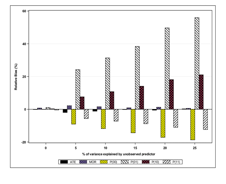
Figure 1: Relative bias of estimated average testing effect (ATE), marginal odds ratio (MOR), and proportion of patients in each potential outcomes subgroup, as the variance of $Y$ explained by an unmeasured predictor of $Y$, $U$, increases and subsequently violation of potential outcomes conditional independence increases (i.e., $\beta_{1}\neq 0$ and $\beta_{2}\neq 0$). Here we assume no interaction between $X_{1}$ and $X_{2}$ (i.e., $\alpha=0$). The true values for ATE is -0.186, MOR is 0.458 and the proportions of patients in four potential outcomes subgroups, $P(00)$, $P(01)$, $P(10)$ and $P(11)$, are 0.212, 0.104, 0.290, and 0.394, respectively.

Lastly, we examine the robustness of the POMI+IND method towards model misspecification. We compare the method with the IPW method. For IPW to work properly, the model for the test assignment $Z$ needs to be correctly specified. Here, we specify the true model for $Z$ as $\textit{logit}[P(Z=1)]=-1.5-X_{1}+0.5X_{2}+2X_{1}\times X_{2}$. However, in data analyses, neither IPW nor POMI+IND methods include the interaction term $X_{1}\times X_{2}$. The simulation results are summarized in Table 5. It shows that IPW gives biased estimates of ATE and MOR and much below $95\%$ coverage rates for their confidence intervals; however, the model misspecification for $Z$ has little impact on estimates from the POMI+IND method. This highlights the need for IPW to specify correct models for $Z$; however, this is not required for the imputation method.

Table 5: Comparing the robustness of POMI+IND and IPW towards model mis-specifications in estimating average testing effect (ATE) and marginal odds ratio (MOR). ESD: empirical standard deviation; SE: standard error; CR: coverage rate of 95$\%$ confidence interval. Here we assume potential outcomes conditional independence (i.e., $\beta_{1}=\beta_{2}=0$) and there is an interaction between $X_{1}$ and $X_{2}$ (i.e., $\alpha\neq 0$).

Quantities	True	Methods	100 $\times$ Bias	ESD	SE	100 $\times$ CR
ATE	-0.186	IPW	-5.98	0.032	0.036	63.6
	-0.186	POMI+IND	0.12	0.032	0.033	95.0
MOR	0.459	IPW	-9.18	0.057	0.052	66.0
	0.459	POMI+IND	0.65	0.065	0.063	94.0

5 Application: the Impact of the RS Assay on Breast Cancer Chemotherapy Selection

The analysis data set includes 2,931 incident breast cancer patients in Georgia and Los Angeles who were diagnosed between 2013-2014 with favorable prognosis (estrogen positive, human epidermal growth factor receptor 2 negative and invasive tumor behavior) Friese ; Li . These patients were chosen because the RS assay has the potential to make a difference in their chemotherapy treatment decisions. The data set comes from three data sources: 1) SEER databases for clinical features; 2) patient survey data from the ICanCare study; 3) the RS assay use and its testing results from the laboratory, Genomic Health, Inc. The outcome of interest is the receipt of chemotherapy (yes/no). The exposure of interest is the receipt of the RS assay (yes/no). The covariates include age (year), tumor grade (1, 2, or 3), tumor size ($\leq$1 cm, $1-2$ cm or $\geq$2 cm), node status (positive or negative), the number of major co-morbidities, menopausal status, and the risk of genetic mutation (low or high), education level (high school or less, some college, graduate degree), race (White, Black, Latino, Asian, other), insurance type (medicaid, medicare, private, other) and family income.

Overall, 35$\%$ of the patients received the RS assay and 27$\%$ received chemotherapy. Among these RS assay testers, the test results showed that $65\%$, $27\%$, and $8\%$ of patients received low-, intermediate- and high-risk scores respectively. We first fit a logistic regression with above covariates without addressing missing data. We find that the factors that are significantly associated with the use of chemotherapy include: the receipt of the RS assay (odds ratio (OR) = 0.42 with 95$\%$ confidence interval (CI): 0.32–0.55), age (OR=0.93, CI: 0.92–0.95), node status (positive vs. negative; OR=7.70, CI: 5.49 – 10.80), tumor grade (2 vs. 1; OR=2.16, CI: 1.60 – 2.93; 3 vs. 1; OR=14.42, CI: 9.82 – 21.17), tumor size (1-2 vs. $\leq$ 1 cm; OR=2.41, CI: 1.72 – 3.36; $\geq$ 2 vs. $\leq$ 1 cm; OR=4.48, CI: 3.09 – 6.48) and the risk of genetic mutation (high vs. low; OR=0.73, CI: 0.54 – 0.99). The C-index from the logistic regression is 0.86. The model was conducted on 2,022 $(69\%)$ patients with complete data. (See Table 12 in Appendix).

We then apply the POMI+IND method to obtain causal estimates. We estimate that the average causal effect of the RS assay testing on chemotherapy (i.e., ATE) is $-10\%$ with its $95\%$ CI of $(-14\%,-7\%)$ and the MOR is 0.59 with its $95\%$ CI of $(0.49,0.70)$. Table 6 presents the proportion of patients in each of the four potential outcome subgroups by overall and by covariates. Overall, it is estimated that the receipt of the RS assay encouraged a change of treatment plan in $9\%(8\%,11\%)$ of patients from no chemotherapy to chemotherapy, and $20\%(17\%,22\%)$ of patients from chemotherapy to no chemotherapy. Hence, the receipt of RS assay has reduced the overall chemotherapy use by $10\%$ and changed the treatment plan for a total of $30\%$ of patients. Regardless of whether they were tested or not, 59$\%$ of patients would never receive chemotherapy and 12$\%$ would always receive chemotherapy.

In addition, we find that, independent of the use of the RS assay, older patients ($\geq$65 years old) are more likely to reject chemotherapy than younger patients ($73\%$ vs. 49$\%$ estimated to be in the “never-treatment” subgroup). We also find that, with the use of the RS assay, patients were more likely to be discouraged from chemotherapy if they had a larger tumor ($36\%$ vs. $19\%$, $8\%$ in the “treatment-discouraged” subgroup for patients with tumor size of $\geq$ 2cm vs. $\leq$ 1cm, 1-2cm) or if they had positive nodes ($40\%$ vs. $15\%$ for patients with positive vs. negative nodes). It is particularly noteworthy that even though the guidelines did not make any recommendations about the use of the RS assay for node-positive patients, $14\%$ of them were offered the RS assay in practice. And in fact these patients were more likely to change their chemotherapy plans after testing with the RS assay than node-negative patients ($46\%$ vs. $25\%$ changed for patients with positive vs. negative nodes).

It is also evident that the RS assay played an influential role in chemotherapy decisions based on how much the results of the assay changed the treatment selections: for patients received a low-risk score, $2\%$ were encouraged to receive chemotherapy vs. $22\%$ discouraged from chemotherapy; for patients received a high-risk score, $34\%$ were encouraged vs. $5\%$ discouraged. In contrast, for patients received an intermediate-risk score, $19\%$ were encouraged vs. $17\%$ discouraged.

Table 6: Estimated proportion of patients in each of the four potential outcomes subgroups defined by the impact of the RS assay on chemotherapy according to patient characteristics, test results and insurance status.

		Estimated Proportion in Each
		Potential Outcomes Subgroup${}_{(95\%\textup{CI})}$
Variables	Categories	Never	Treatment	Treatment	Always
		Treated	Encouraged	Discouraged	Treated
Overall		59(56,61)	9(8,11)	20(17,22)	12(11,14)
Age	$<65$ years old	49(46,51)	9(8,11)	25(23,28)	17(15,19)
	$\geq$65	73(70,76)	10(8,12)	12(10,14)	6(4,7)
node	Negative	69(66,71)	10(9,12)	15(13,16)	7(6,8)
	Positive	20(16,23)	6(4,8)	40(34,46)	35(29,41)
Grade	1	79(76,82)	6(4,8)	13(10,15)	2(1,3)
	2	56(53,59)	10(8,12)	24(21,26)	10(8,12)
	3	15(11,20)	15(11,19)	24(19,29)	46(40,51)
Size	$<1$ cm	79(76,83)	10(8,12)	8(6,9)	3(2,5)
	1-2 cm	59(56,62)	10(8,12)	19(17,22)	12(10,14)
	$\geq$2 cm	31(27,34)	8(6,10)	36 (31,42)	25(21,30)
21-gene score	Low-Risk Score	72(70,75)	2(1,3)	22(20,25)	3(2,5)
	Intermediate-Risk Score	42(37,47)	19(16,23)	17(13,21)	21(17,26)
	High-Risk Score	5(1,10)	34(25,43)	5 (1,9)	56(47,66)
Insurance	Private	57(35,79)	6(0,18)	26(5,46)	11(0,28)
	Medicaid	48(42,54)	10(6,14)	23(18,28)	19(14,25)
	Medicare	75(71,78)	10(7,12)	11(8,13)	5(4,7)

We also fit a multivariable multinomial logistic regression to examine the relationship between several key patient clinical predictors and the potential outcomes subgroup membership. These clinical predictors include tumor node status, tumor grade, tumor size, and age. They are the most important predictors for our study population and have been endorsed by the American Joint Committee on Cancer Kattan . Table 7 listed the estimated probability of patients’ potential outcome subgroup membership as a function of these clinical factors. We estimate that, for patients with negative node, tumor grade $1$, tumor size $\leq$ 1cm, and age$<$65 years old, there was a 7$\%$ chance to be encouraged to receive chemotherapy and 5$\%$ chance to be discouraged from chemotherapy by using the RS assay, an 88$\%$ chance of staying with the decision of no chemotherapy and a 1$\%$ of chance of staying with chemotherapy decision regardless of the use of the RS assay. We also estimate that, for patients with negative node, tumor grade of 3, tumor size of 1-2cm and age $<$ 65 years old, the chances of changing to chemotherapy from no chemotherapy, from no chemotherapy to chemotherapy or staying with chemotherapy or no chemotherapy after the use of the RS assay are 12$\%$, 28$\%$, $52\%$ and $8\%$ respectively. We also found that, generally, patients with a mix of low-risk factors (e.g., smaller tumor size, lower tumor grade, negative node) and high-risk factors (e.g., larger tumor size, higher tumor grade, positive node) for recurrence are more likely to be affected by using the RS assay than patients with either all low-risk or high-risk factors. For example, node-positive patients with small and low-grade tumors are most likely to be discouraged from chemotherapy by using the RS assay. Similarly, node-negative patients with small but high-grade tumor are most likely to be encouraged to take chemotherapy by using the RS assay. In contrast, patients with consistently low (high) risk clinical factors are more likely to remain in the “never treated” (“always treated”) subgroup.

Table 7: Estimated probabilities of potential outcomes subgroup memberships according to patient clinical characteristics based on multinomial logistic regression

			Estimated Probability in Each Subgroup(95%CI)
Tumor	Tumor	Age	Never	Treatment	Treatment	Always
Grade	Size	(yrs)	Treated	Encouraged	Discouraged	Treated
	(cm)
Node Status: Negative
1	$\leq$ 1	$\leq 65$	0.88(0.84,0.92)	0.07(0.04,0.10)	0.05(0.02,0.07)	0.01(0.00,0.01)
1	$\leq$ 1	$\geq 65$	0.93(0.90,0.96)	0.06(0.03,0.09)	0.01(0.00,0.02)	0.00(0.00,0.00)
1	1-2	$\leq 65$	0.75(0.70,0.80)	0.06(0.03,0.09)	0.17(0.13,0.22)	0.02(0.00,0.03)
1	1-2	$\geq 65$	0.92(0.88,0.95)	0.05(0.03,0.08)	0.03(0.01,0.05)	0.00(0.00,0.00)
1	$\geq$ 2	$\leq 65$	0.54(0.43,0.65)	0.04(0.00,0.07)	0.37(0.26,0.47)	0.06(0.01,0.10)
1	$\geq$ 2	$\geq 65$	0.87(0.80,0.94)	0.05(0.00,0.10)	0.07(0.02,0.12)	0.01(0.00,0.02)
2	$\leq$ 1	$\leq 65$	0.75(0.69,0.80)	0.16(0.11,0.20)	0.08(0.04,0.11)	0.02(0.00,0.04)
2	$\leq$ 1	$\geq 65$	0.87(0.82,0.91)	0.10(0.06,0.14)	0.03(0.01,0.05)	0.00(0.00,0.01)
2	1-2	$\leq 65$	0.54(0.49,0.60)	0.13(0.09,0.17)	0.25(0.20,0.30)	0.08(0.05,0.10)
2	1-2	$\geq 65$	0.83(0.79,0.87)	0.09(0.06,0.12)	0.07(0.04,0.10)	0.01(0.00,0.01)
2	$\geq$ 2	$\leq 65$	0.30(0.23,0.37)	0.10(0.05,0.14)	0.46(0.38,0.53)	0.15(0.09,0.20)
2	$\geq$ 2	$\geq 65$	0.69(0.61,0.76)	0.12(0.07,0.17)	0.17(0.11,0.22)	0.03(0.01,0.05)
3	$\leq$ 1	$\leq 65$	0.29(0.15,0.43)	0.30(0.15,0.45)	0.20(0.07,0.32)	0.21(0.08,0.35)
3	$\leq$ 1	$\geq 65$	0.56(0.41,0.71)	0.30(0.16,0.44)	0.08(0.02,0.16)	0.05(0.00,0.11)
3	1-2	$\leq 65$	0.08(0.03,0.12)	0.12(0.07,0.18)	0.28(0.20,0.36)	0.52(0.44,0.61)
3	1-2	$\geq 65$	0.38(0.27,0.50)	0.26(0.16,0.36)	0.17(0.09,0.25)	0.18(0.10,0.27)
3	$\geq$ 2	$\leq 65$	0.04(0.01,0.08)	0.07(0.02,0.12)	0.38(0.27,0.48)	0.51(0.40,0.62)
3	$\geq$ 2	$\geq 65$	0.25(0.12,0.38)	0.21(0.10,0.33)	0.25(0.13,0.36)	0.29(0.16,0.42)
Node Status: Positive
1	$\leq$ 1	$\leq 65$	0.40(0.24,0.55)	0.09(0.01,0.17)	0.39(0.23,0.55)	0.13(0.02,0.24)
1	$\leq$ 1	$\geq 65$	0.65(0.48,0.82)	0.11(0.01,0.21)	0.20(0.07,0.33)	0.04(0.00,0.10)
1	1-2	$\leq 65$	0.20(0.11,0.29)	0.06(0.01,0.11)	0.61(0.49,0.73)	0.13(0.04,0.21)
1	1-2	$\geq 65$	0.56(0.42,0.71)	0.10(0.02,0.18)	0.29(0.16,0.43)	0.04(0.00,0.09)
1	$\geq$ 2	$\leq 65$	0.11(0.04,0.18)	0.03(0.00,0.06)	0.63(0.49,0.77)	0.24(0.11,0.37)
1	$\geq$ 2	$\geq 65$	0.44(0.24,0.63)	0.07(0.00,0.15)	0.37(0.19,0.55)	0.12(0.01,0.26)
2	$\leq$ 1	$\leq 65$	0.23(0.10,0.35)	0.09(0.01,0.17)	0.39(0.23,0.55)	0.30(0.13,0.46)
2	$\leq$ 1	$\geq 65$	0.47(0.29,0.64)	0.09(0.00,0.17)	0.34(0.17,0.50)	0.11(0.01,0.22)
2	1-2	$\leq 65$	0.09(0.05,0.14)	0.05(0.02,0.08)	0.51(0.42,0.60)	0.35(0.26,0.43)
2	1-2	$\geq 65$	0.34(0.23,0.45)	0.07(0.02,0.13)	0.45(0.34,0.57)	0.13(0.05,0.20)
2	$\geq$ 2	$\leq 65$	0.05(0.02,0.07)	0.03(0.00,0.05)	0.52(0.43,0.61)	0.40(0.31,0.50)
2	$\geq$ 2	$\geq 65$	0.21(0.12,0.30)	0.07(0.02,0.12)	0.49(0.37,0.60)	0.24(0.14,0.33)
3	$\leq$ 1	$\leq 65$	0.03(0.00,0.09)	0.11(0.00,0.25)	0.17(0.01,0.35)	0.69(0.43,0.94)
3	$\leq$ 1	$\geq 65$	0.13(0.00,0.31)	0.18(0.00,0.40)	0.18(0.01,0.38)	0.50(0.19,0.82)
3	1-2	$\leq 65$	0.01(0.00,0.02)	0.05(0.00,0.10)	0.16(0.06,0.26)	0.79(0.67,0.90)
3	1-2	$\geq 65$	0.06(0.00,0.14)	0.13(0.01,0.25)	0.19(0.06,0.32)	0.61(0.43,0.80)
3	$\geq$ 2	$\leq 65$	0.01(0.00,0.02)	0.04(0.00,0.07)	0.19(0.10,0.28)	0.77(0.67,0.86)
3	$\geq$ 2	$\geq 65$	0.04(0.00,0.09)	0.10(0.01,0.19)	0.18(0.07,0.28)	0.68(0.53,0.83)

We further examine how robust our analysis results are towards the violation of the potential outcomes conditional independence assumption (Assumption 4). Since $Y_{0}$ and $Y_{1}$ are not observed simultaneously in our data, we cannot evaluate this conditional independence assumption nor estimate the correlation between $Y_{0}$ and $Y_{1}$ based on our data. We artificially induce a correlation by simulating an additional predictor U of Y that is not in the data set, and examine how sensitive our analyses are towards the correlation between $Y_{0}$ and $Y_{1}$. Since $U$ is a predictor of $Y$, $U$ is a common predictor of both $Y_{0}$ and $Y_{1}$. Since U is not observed or adjusted for, this induces the correlation between $Y_{0}$ and $Y_{1}$. The more correlated $Y_{0}$ and $Y_{1}$ are, the more severe the violation of the conditional independence assumption is. We let $U=(-0.267+Y)*b_{1}+e$, where $Y$ is the observed receipt of chemotherapy and $e\sim$ Normal$(0,\sigma^{2})$. Since $26.7\%$ of patients were observed to receive chemotherapy, we choose -0.267 in this equation to ensure that the mean of $U$ equals $0$. We vary $b_{1}$ to change the association between $U$ and $Y$ and examine how it affects the causal estimates. For each $b_{1}$ value, we re-impute the missing values conditional on the same set of covariates listed previously and the simulated predictor $U$, and then re-estimate the causal quantities of interest using the POMI+IND method. Figure 2 plots the estimates according to a wide range of the extent of variation in $Y$ explained by $U$, which is estimated by a non-linear mixed effect model with $U$ as a random effect Browne . As the extent of variation in $Y$ explained by $U$ increases, the proportions of patients in the “never treated” and “always treated” subgroups increase, and the proportions in other two subgroups decrease. Subsequently, the overall influence of 21-gene assay on chemotherapy receipts decreases. We also observe that MOR and ATE only increase slightly. Overall, these causal estimates are not very sensitive towards $U$.

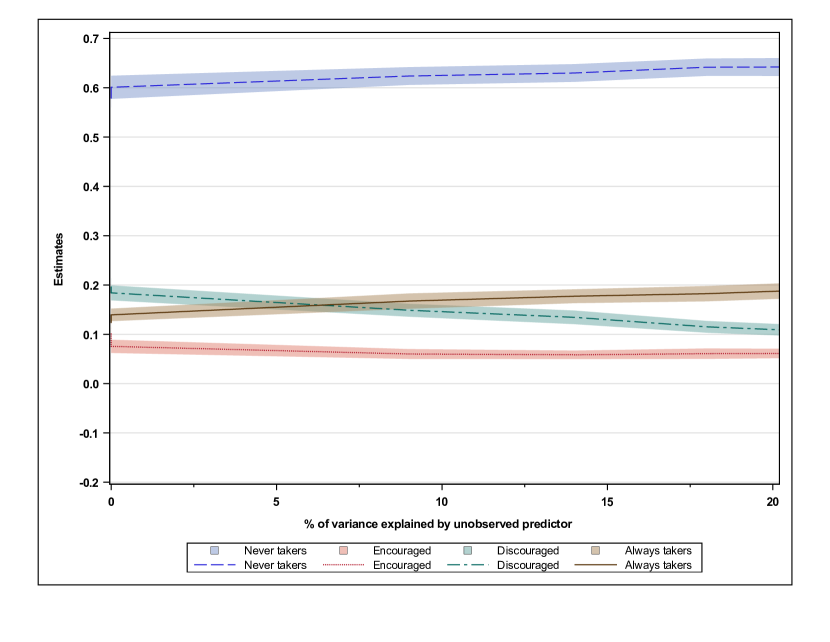
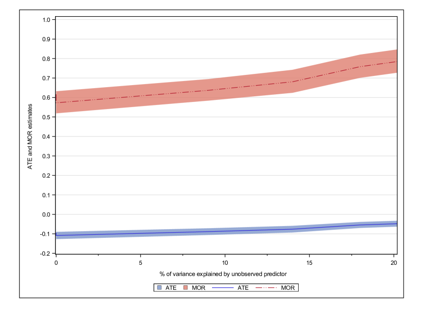
Figure 2: Estimated proportion of patients in each potential outcomes subgroup, ATE and MOR, as the variance of $Y$ explained by an unmeasured predictor of $Y$, $U$, increases and the subsequent violation of the potential outcomes conditional independence assumption increases.

6 Discussion

We proposed a potential outcomes framework to measure the influence of medical testing on treatment selection, stratifying patients into four potential outcomes subgroups based on whether the test has any impact on treatments election (either undergoing the treatment or not), and whether the test encourages or discourages treatment selection. This framework captures well the differential causal effect of testing on treatment selection for different patient subgroups, and allows us to examine the distribution of these subgroups and characteristics associated with these subgroup memberships. The classification suggests targets for more efficient utilization of medical tests. With advanced tests designed to support precision medicine becoming increasingly available and increasing concern for over-testing Schnipper , the causal estimates produced from this framework become more relevant. The framework also allows us to estimate many traditional causal quantities of interest (e.g., average causal effects, marginal odds ratios) on which existing causal inference methods more often focus. By taking advantage of the connection between missing data and causal inference, we can simultaneously implement the causal framework as well as handle missing data in the observable variables (i.e., due to non-response). We also explore the advantages of incorporating unique features of causal inference assumptions in the data imputation process. These assumptions are often made in causal inference literature, but cannot be estimated or verified from the data. Simulation studies suggested that the proposed methods provide reasonably accurate inference. Additionally, the explicit incorporation of the causal assumptions in the data imputation process can improve precision for some causal estimates. We also find that bias can occur for some causal estimates when the potential outcomes conditional independence assumption is violated, which can be assessed through sensitivity analyses. The proposed framework was then used to examine how the most commonly used genomic test in the United States, 21-gene assay, impacts the use of chemotherapy among breast cancer patients.

Existing research has often focused on estimating the overall relationship between medical testing and treatment options in a population. For example, breast magnetic resonance imaging has been found to be associated with receiving a mastectomy instead of breast conserving surgery (adjusted odds ratio = 1.21) Killelea . In another example, it is found that $55\%$ of women with invasive breast cancer and positive HER2 genetic testing results received trastuzumab treatment Goddard . Although this information is of interest, the average effect of testing on treatment choice may not apply equally across subgroups of patients who may not benefit from (or, may be harmed by) testing. Hence, it is important to recognize that a medical test can have different influences on treatment decisions for different patients; i.e., there may be effect heterogeneity of testing on treatment. We proposed the use of potential outcomes subgroups to classify patients by the presence (vs. absence) and direction of the effect of testing on treatment decisions. Patients are classified into one of the four groups: 1) never treated; 2) treatment encouraged; 3) treatment discouraged; 4) always treated. These subgroups naturally capture the effect heterogeneity of medical testing on treatment decisions. Additionally, we investigated how patients’ membership in these subgroups may be driven by patient characteristics or systemic factors. Such classification would suggest targets for improving the utilization of medical tests and the allocation of limited resources. For example, in the data analyses, we found that patients with positive nodes were more influenced by the testing and more of these patients were discouraged from receiving chemotherapy than patients with negative nodes, even though guidelines make no recommendations for how to use the 21-gene assay in node-positive patients. We also find that patients with a mix of low and high risk factors were more likely to be influenced by the use of 21-gene assay, and the tests were more likely to either encourage or discourage these patients for chemotherapy use. Given that the test was recommended to aid decision-making in people with intermediate risk of recurrence, our results show that efforts to ensure that the patients with a mix of low and high risk factors are offered testing are likely to produce substantial changes in plans and maximize the utility of the test.

Our methods differ from traditional latent class models, which usually deal with multiple or longitudinal outcomes and do not classify patients by potential outcomes. Subgroup analysis or adding interaction terms can also investigate effect heterogeneity; however, these approaches require us to pre-specify variables that modify effect and suffer from false discovery rate Fink . In summary, standard analyses cannot provide the classification targeted by our methods. Our methods of analyzing heterogeneous testing effect using the potential outcomes subgroups approach are at the individual level. For each patient, the testing effect on treatment is obtained by comparing her underlying tendency of receiving treatment with vs. without a given test. Our approach may be complementary to the standard analyses based on known effect modifiers. Further discussions of individual heterogeneous treatment effects are discussed by others Zhang ; Poulson ; Egleston .

We proposed the use of multiple imputation methods to impute the missing potential outcomes for each patient ($Y_{0}$ or $Y_{1}$) since we do not observe two potential outcomes of the same patient simultaneously. Subsequently, we can classify patients into four potential outcomes subgroups according to individual heterogeneous treatment effects. We chose the sequential regression multiple imputation method. It has the advantages of accommodating many different data types and structure compared with other missing data methods Ambler . The main uncertainty in theoretical justification for this method is the likely incompatibility between the assumed conditional models and the true conditional models derived from the joint conditional distributions Raghu . However, many simulation studies have demonstrated the robustness of this method towards possible misspecifications of the assumed conditional models Ambler .

Our methods have the advantage of imputing missing potential outcomes and regular missing values in the observable variables simultaneously during the data imputation process. This is more convenient and faster than most of other causal inference methods in the presence of missing data, which will likely need to handle the missing data problem first using multiple imputation methods before applying causal inference methods and combining analysis results across multiple imputed data sets.

The use of multiple imputation methods utilizes the close connection between causal inference and missing data framework, since the causal inference problems here are essentially a missing data problem. However, there are some unique features of causal inference that are different from the regular missing data problems in our context. First, causal assumptions are unique. Even though there is no information from the data to test the validity of the assumptions regarding ignorability or potential outcomes conditional independence, we demonstrate that the explicit incorporation of these causal assumptions into the data imputation process can increase the precision of some of our causal estimates such as the proportion of patients in each of the potential outcomes subgroups. Second, we find that the violation of the potential outcomes conditional independence assumption does not have much impact on traditional causal quantities such as the average causal effect or marginal odds ratio. However, it does impact the causal quantities regarding the potential outcomes subgroups, which concern the joint distribution of the potential outcomes. As the correlation between two potential outcomes increases, patients in the treatment-encouraged and treatment-discouraged subgroups become fewer. Since there is no information from the empirical data about the validity of this assumption, we proposed a method to conduct sensitivity analyses to relax this assumption and evaluate the impact of violation of this assumption. Our proposed sensitivity analyses are closely related to the random effect models proposed by Zhang et al. Zhang , which use random effects to induce the correlation between $Y_{0}$ and $Y_{1}$. Here we used an unmeasured predictor of $Y$ to induce the correlation. Third, $Z$ is the missing data indicator for $Y_{0}$ and $Y_{1}$. With an MAR assumption, multiple imputation does not usually need to include the missing indicator Van . However, $Z$ is also the exposure of interest. And it is a function of the covariate $X_{2}$, which is partially missing. Hence, for multiple imputation of $X_{2}$ to work properly, the imputation model for $X_{2}$ needs to include $Z$ to satisfy the MAR assumption. This explains why POMI-Z performs more poorly in our simulations compared with methods including $Z$ in the imputation models. Fourth, a post-exposure variable (e.g., testing results) that is correlated with the outcome is not usually utilized in the causal inference methods because it can be in the causal pathway between the exposure and outcome. However, it is usually used in the multiple imputation process and not treated differently from other variables. Our study finds that the incorporation of a post-exposure variable in the multiple imputation process still generates valid causal estimates. In fact, it did not make much difference whether or not we included the post-exposure variable in our simulations. However, we believe that if the post-exposure variable is correlated with variables that have more missingness, the utilization of the post-exposure variable will increase precision. In our simulations, there is only $10\%$ missingness in the variable $Y$, a correlate of the post-exposure variable $R$; hence, the incorporation of $R$ in the imputation process did not provide noticeable efficiency gain. Lastly, we find that our POMI methods do not require the need to correctly specify the model for the exposure to obtain valid causal estimates; however, a propensity-score based causal method usually does. This feature occurs because the POMI methods do not require one to model the exposure but only to provide a correct predictive model for the outcome. Our methods can be implemented through IVEware in SAS, or through the MICE (Multivariate Imputation by Chained Equations) package in R. We have provided code examples in GitHub at https://github.com/yunliyunli/POMI.

In summary, we proposed a potential outcomes framework to classify patients according to the differential causal effect of medical testing on treatment selection for different individual patients. It has the potential to be very useful in examining effect heterogeneity of medical testing on treatment selection and in proposing targets for the optimal use of medical tests. Future research includes conducting more sensitivity analyses on the causal assumptions and improving the efficiency for these causal quantities of interest.

The authors declared no potential conflicts of interest with respect to the research, authorship, and/or publication of this article.

This work was supported by the National Cancer Institute through grants P01CA163233, CA46592, CA129102 and U057141.

Yun Li and Irina Bondarenko contribute equally.

7 Appendix

8 Additional Simulation Results with Different Sample Sizes

Additional simulations were conducted using a sample size of 250 to evaluate the impact of sample size. Results are summarized in Tables 8-9.

Table 8: Additional simulations: comparison of five methods in estimating average testing effect (ATE), and marginal odds ratios (MOR) when N=250. ESD: empirical standard deviation; SE: average standard error; CR: coverage rate of 95$\%$ confidence interval. Here we assume potential outcomes conditional independence and no interaction between $X_{1}$ and $X_{2}$ (i.e., $\alpha=\beta_{1}=\beta_{2}=0$).

Quantities	Methods	True	100 $\times$ Bias	ESD	SE	100 $\times$ CR
ATE	POMI-Z	-0.186	2.9	0.071	0.076	93.2
	POMI	-0.186	1.6	0.070	0.082	94
	POMI+IND	-0.186	0.8	0.068	0.066	91.4
	POMI+IND-R	-0.186	0.6	0.066	0.066	92.4
	IPW	-0.186	-0.5	0.074	0.077	93.8
MOR	POMI-Z	0.458	7.7	0.169	0.187	91.8
	POMI	0.458	4.7	0.161	0.192	95.6
	POMI+IND	0.458	3.1	0.147	0.141	90.6
	POMI+IND-R	0.458	2.4	0.143	0.141	92.8
	IPW	0.458	2.1	0.146	0.156	93.6

Table 9: Additional simulation: comparison of five methods in estimating the proportion of patients in each potential outcome subgroup when N=250. ESD: empirical standard deviation; SE: standard error; CR: coverage rate of 95$\%$ confidence interval. Here we assume potential outcomes conditional independence and no interaction between $X_{1}$ and $X_{2}$ (i.e., $\alpha=\beta_{1}=\beta_{2}=0$).

Quantities	Methods	True	100 $\times$ Bias	ESD	SE	100 $\times$ CR
P(00)	POMI-Z	0.21	0.49	5.527	7.529	94.4
	POMI	0.21	0.44	4.703	7.934	98.2
	POMI+IND	0.21	-0.27	3.576	4.046	95.4
	POMI+IND-R	0.21	-0.27	3.654	4.063	95.2
	IPW	–	–	–	–	–
P(01)	POMI-Z	0.10	3.08	4.737	6.978	91.6
	POMI	0.10	2.82	3.965	7.391	98
	POMI+IND	0.10	0.60	2.933	3.368	95
	POMI+IND-R	0.10	0.51	2.839	3.383	95.8
	IPW	–	–	–	–	–
P(10)	POMI-Z	0.29	-1.11	6.328	8.268	94
	POMI	0.29	-0.45	5.724	8.988	98.4
	POMI+IND	0.29	-0.24	4.511	4.700	93.2
	POMI+IND-R	0.29	-0.04	4.438	4.712	94.2
	IPW	–	–	–	–	–
P(11)	POMI-Z	0.39	-0.43	6.261	8.080	95.4
	POMI	0.39	-0.39	5.211	8.865	99.4
	POMI+IND	0.39	-0.08	4.073	4.689	96.8
	POMI+IND-R	0.39	-0.20	4.001	4.670	96.2
	IPW	–	–	–	–	–

Additional simulations were conducted using a sample size of 500 to evaluate the impact of sample size. Results are summarized in Tables 10-11.

Table 10: Additional simulation: comparison of five methods in estimating average testing effect (ATE), and marginal odds ratios (MOR) when N=500. ESD: empirical standard deviation; SE: average standard error; CR: coverage rate of 95$\%$ confidence interval. Here we assume potential outcomes conditional independence and no interaction between $X_{1}$ and $X_{2}$ (i.e., $\alpha=\beta_{1}=\beta_{2}=0$).

Quantities	Methods	True	100 $\times$ Bias	ESD	SE	100 $\times$ CR
ATE	POMI-Z	-0.186	2.0	0.048	0.047	90.6
	POMI	-0.186	0.4	0.047	0.050	93.8
	POMI+IND	-0.186	0.1	0.048	0.047	91.6
	POMI+IND-R	-0.186	0.1	0.049	0.047	92
	IPW	-0.186	-0.9	0.052	0.054	96
MOR	POMI-Z	0.458	4.8	0.110	0.105	90.2
	POMI	0.458	1.6	0.099	0.104	94.2
	POMI+IND	0.458	0.9	0.101	0.096	91.6
	POMI+IND-R	0.458	0.8	0.100	0.096	92.6
	IPW	0.458	0.4	0.101	0.106	95.2

Table 11: Additional simulation: comparison of five methods in estimating the proportion of patients in each potential outcome subgroup when N=500. ESD: empirical standard deviation; SE: standard error; CR: coverage rate of 95$\%$ confidence interval. Here we assume potential outcomes conditional independence and no interaction between $X_{1}$ and $X_{2}$ (i.e., $\alpha=\beta_{1}=\beta_{2}=0$).

Quantities	Methods	True	100 $\times$ Bias	ESD	SE	100 $\times$ CR
P(00)	POMI-Z	0.21	0.34	4.315	5.948	96
	POMI	0.21	0.03	3.737	6.154	97.4
	POMI+IND	0.21	-0.07	2.734	2.863	93.8
	POMI+IND-R	0.21	-0.07	2.777	2.925	93.2
	IPW	–	–	–	–	–
P(01)	POMI-Z	0.10	1.50	1.501	0.954	95.4
	POMI	0.10	0.96	0.963	0.976	97.6
	POMI+IND	0.10	0.23	0.228	0.954	95.4
	POMI+IND-R	0.10	0.29	0.291	0.962	96.2
	IPW	–	–	–	–	–
P(10)	POMI-Z	0.29	-0.84	4.522	6.278	95.2
	POMI	0.29	0.11	4.167	6.523	98.6
	POMI+IND	0.29	0.14	3.289	3.357	93.2
	POMI+IND-R	0.29	0.23	3.303	3.387	93.4
	IPW	–	–	–	–	–
P(11)	POMI-Z	0.39	-0.47	4.231	6.325	98
	POMI	0.39	-0.59	3.934	6.312	99
	POMI+IND	0.39	-0.30	2.928	3.296	95.6
	POMI+IND-R	0.39	-0.45	2.911	3.302	96
	IPW	–	–	–	–	–

9 Logistic regression Results for Chemotherapy Use

The results from the logistic regression model are presented in Table 12.

Table 12: Logistic Regression Results for Chemotherapy Use Based on Observed Variables. RS Assay: 21-Gene Assay

Variable	Categories	OR	$95\%$ CI
Receipt of RS Assay	Yes vs. No	0.42	0.32	0.55
Tumor grade	2	2.16	1.60	2.93
(Ref: 1)	3	14.42	9.82	21.17
Age (year)		0.93	0.92	0.95
Tumor size (cm)	$1-2$	2.41	1.72	3.36
(Ref: $\leq$1)	$\geq$ 2	4.48	3.09	6.48
Positive Node Status	Yes vs. No	7.70	5.49	10.80
High Risk of Genetic Mutation	Yes vs. No	0.73	0.54	0.99
Number of Comorbidities		1.04	0.84	1.28
Race	Black	1.05	0.73	1.51
(Ref: White)	Latino	0.73	0.50	1.07
	Asian	0.77	0.47	1.24
	Other	1.12	0.35	3.58
Education	Some college	0.87	0.60	1.26
(Ref: High school or less)	Graduate	0.90	0.61	1.32
Family Income		1.02	0.94	1.11
Insurance	None	0.78	0.19	3.25
(Ref: Private)	Medicaid	1.39	0.87	2.23
	Medicare	0.92	0.62	1.36
	Other	1.56	0.44	5.51

10 Variance Estimates of Marginal Odds Ratio

The MOR is defined as MOR= $[P_{1}/(1-P_{1})]/[P_{0}/(1-P_{0})]$. Since MOR is skewed and bounded to be positive, we use log transformation to make it more symmetric so that we can use the delta method to obtain the variance estimate of $log(\widehat{MOR})$ first. Let $log(\widehat{MOR})_{d}$ be the point estimate of log(MOR) in the $d$th imputed data set where $d=1,\ldots\,D$. The combined multiple imputation estimate of log(MOR) across D imputed data sets is

$$\overline{log(\widehat{MOR})}=\frac{1}{D}\sum_{d=1}^{D}log(\widehat{MOR})_{d}.$$

For the variance of $log(\widehat{MOR})$ in the dth imputed data set denoted by $W_{d}$, we calculate it using the delta method as below:

$$\begin{bmatrix}\frac{\partial log(\widehat{MOR})}{\partial p_{1}}&\frac{\partial log(\widehat{MOR})}{\partial p_{0}}\end{bmatrix}\times Var(\widehat{p}_{1},\widehat{p}_{0})\times\begin{bmatrix}\frac{\partial log(\widehat{MOR})}{\partial p_{1}}\\ \frac{\partial log(\widehat{MOR})}{\partial p_{0}}\end{bmatrix}$$

$$=\frac{1}{N}\begin{bmatrix}\frac{1}{\widehat{p}_{1}(1-\widehat{p}_{1})}&\frac{-1}{\widehat{p}_{0}(1-\widehat{p}_{0})}\end{bmatrix}\times\begin{bmatrix}\widehat{p}_{1}(1-\widehat{p}_{1})&\widehat{p}_{11}-\widehat{p}_{0}\widehat{p}_{1}\\ \widehat{p}_{11}-\widehat{p}_{0}\widehat{p}_{1}&\widehat{p}_{0}(1-\widehat{p}_{0})\end{bmatrix}\times\begin{bmatrix}\frac{1}{\widehat{p}_{1}(1-\widehat{p}_{1})}\\ \frac{-1}{\widehat{p}_{0}(1-\widehat{p}_{0})}\end{bmatrix}$$

$$=\frac{\widehat{p}_{0}+\widehat{p}_{1}-(\widehat{p}_{0}-\widehat{p}_{1})^{2}-2\widehat{p}_{11}}{N\widehat{p}_{0}\widehat{p}_{1}(1-\widehat{p}_{0})(1-\widehat{p}_{1})}$$ (11)

Averaging over multiple imputed data sets, we calculate the average within-imputation variance as $\overline{W}=\sum_{d=1}^{D}W_{d}/D$. For between-imputation variance denoted by $B$, we have $B=\sum_{d=1}^{D}\left[log(\widehat{MOR})_{d}-\overline{log(\widehat{MOR})}\right]^{2}/(D-1)$. The multiple imputation estimate of the variance of $\overline{log(\widehat{MOR})}$ is $V=\overline{W}+(1+\frac{1}{D})B$.

After we obtain the variance of the estimated log(MOR), we can then use the delta method to obtain the variance of estimated MOR such that $Var(\widehat{MOR})=\exp\left\{2\left[log(\widehat{MOR})\right]\right\}\times Var\left[log(\widehat{MOR})\right]$.

References

- (1) Brill S. Bitter Pill -– The Absurd Costs of American Health Care. Time Magazine. 2013.
- (2) Albain KS, Barlow WE, Shak S, Hortobagyi GN, Livingston RB, Yeh IT, Ravdin P, Bugarini R, Baehner FL, Davidson NE, Sledge GW, Winer EP, Hudis C, Ingle JN, Perez EA, Pritchard Kl, Shepherd L, Gralow JR, Yoshizawa C, Allred DC, Osborne CK, Hayes DF. Prognostic and predicfive value of the 21-gene recurrence score assay in postmenopausal women with node-positive, oestrogen-receptor-positive breast cancer on chemotherapy: A retrospective analysis of a randomised trial. Lancet Oncol. 2010; 11(1):55-65: PMID 20005174.
- (3) Schnipper LE, Lyman GH, Blayney DW, et al: American Society of Clinical Oncology 2013 top five list in oncology. J Clin Oncol. 2013; 31:4362-70.
- (4) Paik S, Shak S, Tang G, Kim C, Baker J, Cronin M, Baehner FL, Walker MG, Watson D, Park T, Hiller W, Fisher ER, Wickerham DL, Bryant J, Wolmark N. A multigene assay to predict recurrence of tamoxifentreated, node-negative breast cancer. N Engl J Med. 2004;351(27):2817-26: PMID 15591335.
- (5) Habel LA, Shak S, Jacobs MK, Capra A, Alexander C, Pho M, Baker J, Walker M, Watson D, Hackett J, Blick NT, Greenberg D, Fehrenbacher L, Langholz B, Quesenberry CP. A population-based study of tumor gene expression and risk of breast cancer death among lymph node-negative patients. Breast Cancer Res. 2006;8(3):R25: PMID 16737553.
- (6) Paik S, Tang G, Shak S, Kim C, Baker J, Kim W, Cronin M, Baehner FL, Watson D, Bryant J, Costanfino JP, Geyer CE, Jr., Wickerham DL, Wolmark N. Gene expression and benefit of chemotherapy in women with node-negative, estrogen receptor-posifive breast cancer. J Clin Oncol. 2006; 24(23):3726-34: PMID 16720680.
- (7) Dowsett M, Cuzick J, Wale C, Forbes J, Mallon EA, Salter J, Quinn E, Dunbier A, Baum M, Buzdar A, Howell A, Bugarini R, Baehner FL, Shak S. Prediction of risk of distant recurrence using the 21-gene recurrence score in node-negafive and node-positive postmenopausal pafients with breast cancer treated with anastrozole or tamoxifen: a TransATAC study. J Clin Oncol. 2010;28(11): 1829-34: PMID 202122
- (8) Goldstein LJ, Gray R, Badve S, Childs BH, Yoshizawa C, Rowley S, Shak S, Baehner FL, Ravdin PM, Davidson NE, Sledge GW, Jr., Perez EA, Shulman LN, Martino S, Sparano JA. Prognostic ufility of the 21-gene assay in hormone receptor-positive operable breast cancer compared with classical clinicopathologic features. J Clin Oncol 2008;26(25):4063-71: PMID 18678838.
- (9) Harris L, Fritsche H, Mennel R, Norton L, Ravdin P, Taube S, Somerfield MR, Hayes DF, Bast RC, Jr.American Society of Clinical Oncology 2007 update of recommendafions for the use of tumor markers in breast cancer. J Clin Oncol. 2007;25(33):5287-312: PMID 17954709.
- (10) National Comprehensive Cancer Network, http://www.nccn.org/professionals.
- (11) Sparano, J. A., Gray, R. J., Makower, D. F., Pritchard, K. I., Albain, K. S., Hayes, D. F., … Sledge, G. W. (2018). Adjuvant chemotherapy guided by a 21-gene expression assay in breast cancer. New England Journal of Medicine, 379(2), 111-121. https://doi.org/10.1056/NEJMoa1804710
- (12) Manjelievskaia J, Brown D, McGlynn KA, Anderson W, Shriver CD, Zhu K. Chemotherapy Use and Survival Among Young and Middle-Aged Patients With Colon Cancer. JAMA Surg. 2017;152(5):452–459. doi:https://doi.org/10.1001/jamasurg.2016.5050
- (13) Bosco JL, Silliman RA, Thwin SS, Geiger AM, Buist DS, Prout MN, Yood MU, Haque R, Wei F, Lash TL. A most stubborn bias: no adjustment method fully resolves confounding by indication in observational studies. Journal of Clinical Epidemiology. 2010;63(1):64–74.
- (14) Salas M, Hofman A, Stricker BH. Confounding by indication: an example of variation in the use of epidemiologic terminology. American Journal of Epidemiology. 1999;149(11):981–983.
- (15) HOLLAND, P. Statistics and causal inference (with discussion). J. Amer. Statist. Assoc.. (1986); 81:945–970.
- (16) Frangakis, C. E. and Rubin, D. B. Principal stratification in casual inference. Biometrics. 2002; 58, 21–29.
- (17) Huang Y, Gilbert PB, Wolfson J. Design and estimation for evaluating principal surrogate markers in vaccine trials. Biometrics. 2013; 69(2):301-309.
- (18) Li Y, Taylor JM, Elliott MR. A bayesian approach to surrogacy assessment using principal stratification in clinical trials. Biometrics. Jun 2010;66(2):523-531.
- (19) Roy J, Hogan JW, Marcus BH. Principal stratification with predictors of compliance for randomized trials with 2 active treatments. Biostatistics. 2008;9(2):277-289.
- (20) Jae-kwang Kim, Emily Berg, Taesung Park. Statistical Matching using Fractional Imputation. arXiv:1510.03782 [stat.ME]
- (21) Pier Luigi Conti, Daniela Marella, Mauro Scanu. How far from identifiability? A systematic overview of the statistical matching problem in a non parametric framework. Communications in Statistics - Theory and Methods. 2017; 46:2, 967-994, DOI: 10.1080/03610926.2015.1010005
- (22) Rubin DB. Inference and missing data. Biometrika. 1976;63(3):581–592
- (23) Taylor, L., Zhou, X. (2009). Multiple Imputation Methods for Treatment Noncompliance and Nonresponse in Randomized Clinical Trials. Biometrics, 65(1), 88-95.
- (24) Gutman R, Rubin DB. Estimation of causal effects of binary treatments in unconfounded studies. Stat Med. 2015;34(26):3381–3398.
- (25) Bondarenko I and Raghunathan T: Multiple Imputation for Causal Inference. 2010. In JSM Proceedings, Survey Research Methods Section. Alexandria, VA: American Statistical Association. 3934-3944.
- (26) Westreich D, Edwards JK, Cole SR, Platt RW, Mumford SL, Schisterman EF. Imputation approaches for potential outcomes in causal inference. Int J Epidemiol. 2015;44(5):1731–1737.
- (27) , T., Elliott, M.R., Little, R.J.A. Penalized Spline of Propensity Methods for Treatment Comparison. Journal of the American Statistical Association (with discussion). 2019; 114, 1-38.
- (28) Miao X., Li X., Gilbert P.B., Chan I.S.F. (2013) A Multiple Imputation Approach for the Evaluation of Surrogate Markers in the Principal Stratification Causal Inference Framework. In: Lee ML., Gail M., Pfeiffer R., Satten G., Cai T., Gandy A. (eds) Risk Assessment and Evaluation of Predictions. Lecture Notes in Statistics, vol 215. Springer, New York, NY
- (29) Ding, P, and Li, F. Causal inference: a missing data perspective. Statistical Science. 2018; 33(2), 214-237. [DOI — arXiv]
- (30) Westreich D, Edwards JK, Cole SR, Platt RW, Mumford SL, Schisterman EF. Imputation approaches for potential outcomes in causal inference. Int J Epidemiol. 2015;44(5):1731–1737. doi:10.1093/ije/dyv135
- (31) Friese CR, Li Y, Bondarenko I, Hofer T; Ward KC, Hamilton AS, Deapen D, Kurian AW, Katz SJ. Chemotherapy Decisions and Patient Experience with the Recurrence Score Assay for Early-Stage Breast Cancer. Cancer. (2017); 123(1):43-51.
- (32) Li Y, Kurian AW, Bondarenko I, Taylor J, Ward KC, Hamilton AS, Katz SJ, Hofer TP. The influence of 21-gene recurrence score assay on chemotherapy use in a population-based sample of breast cancer patients. Breast Cancer Res Treat. (2017); 161(3):587-595.
- (33) Holland, P. W. (1986). Statisticsand causal inference. Journal of the American statistical Association, 81(396), 945-960.
- (34) Raghunathan T, Lepkowski J, VanHoewyk J, Solenberger P. A multivariate technique for multiply imputing missing values using a sequence of regression models. Survey Methodology. 2001;27(1):85-96.
- (35) van Buuren S. Multiple imputation of discrete and continuous data by fully conditional specification. Statistical Methods in Medical Research. Jun 2007;16(3):219-242.
- (36) Statistical Analysis With Missing Data. Roderick J. A. Little and Donald B. Rubin. New York: John Wiley & Sons, 2019.
- (37) Rubin, D.B. (1980). Randomization analysis of experimental-data - the Fisher randomziation test - comment. Journal of American Statistical Association 75, 591–593.
- (38) Rubin, D.B. (1978). Bayesian-inference for causal effects - role of randomization. The Annals of Statistics 6, 34–58.
- (39) Zhang, Z, Wang, C, Nie, L Assessing the heterogeneity of treatment effects via potential outcomes of individual patients. J R Stati Soc C 2013; 62: 687–704.
- (40) Efron B, Feldman D. Compliance as an explanatory variable in clinical trials. Journal of the American Statistical Association 1991; 86(413):9–17.
- (41) Daniels, M. J., Roy, J. A., Kim, C. , Hogan, J. W. and Perri, M. G. (2012), Bayesian Inference for the Causal Effect of Mediation. Biometrics, 68: 1028-1036.
- (42) Rubin, D. B. and Schenker, N. (1986). Multiple imputation for interval estimation from simple random samples with ignorable nonresponse. Journal of the American Statistical Association, 81, 366–374
- (43) Kennickell AB (1991). “Imputation of the 1989 survey of consumer finances: Stochastic relaxation and multiple imputation.” ASA 1991 Proceedings of the Section on Survey ResearchMethods, pp. 1–10.
- (44) Robins, J. (1989) The control of confounding by intermediate variables. Statist. Med., 8, 679–701. Bond
- (45) Bondarenko, I., and Raghunathan, T. ( 2016) Graphical and numerical diagnostic tools to assess suitability of multiple imputations and imputation models. Statist. Med., 35: 3007– 3020. doi: 10.1002/sim.6926.
- (46) Horvitz, D. G.; Thompson, D. J. (1952) A generalization of sampling without replacement from a finite universe, Journal of the American Statistical Association, 47, 663–685
- (47) Kattan MW, Hess KR, Amin MB, Lu Y, Moons KGKattan , Gershenwald JE, et al. American Joint Committee on Cancer acceptance criteria for inclusion of risk models for individualized prognosis in the practice of precision medicine. CA Cancer J Clin. 2016;66(5):370–4.
- (48) W. J. Browne, S. V. Subramanian, K. Jones, H. Goldstein, 2005. Variance partitioning in multilevel logistic models that exhibit overdispersion. Journal of the Royal Statistical Society Series A, Royal Statistical Society, vol. 168(3), pages 599-613, July.
- (49) Killelea BK, Long JB, Chagpar AB, et al. Trends and clinical implications of preoperative breast MRI in Medicare beneficiaries with breast cancer. Breast Cancer Research and Treatment. Aug 2013;141(1):155-163.
- (50) Goddard KA, Bowles EJ, Feigelson HS, et al. Utilization of HER2 genetic testing in a multi-institutional observational study. The American Journal of Managed Care. Nov 2012;18(11):704-712.
- (51) Fink G, McConnell M, Vollmer S. Testing for heterogeneous treatment effects in experimental data: false discovery risks and correction procedures. Journal of Development Effectiveness. 2014/01/02 2014;6(1):44-57.
- (52) Poulson RS, Gadbury GL, Allison DB. Treatment heterogeneity and individual qualitative interaction. Am Statistn. 2012; 66:16–24.
- (53) Egleston, B.L., Uzzo, R.G., Wong, Y.N. Latent class survival models linked by principal stratification to investigate heterogeneous survival subgroups among individuals with early stage kidney cancer. Journal of the American Statistical Association; 2017 in press. doi: 10.1080/01621459.2016.1240078
- (54) Ambler G, Omar RZ, Royston P. . A comparison of imputation techniques for handling missing data predictor values in a risk model with a binary outcome. Statist. Meth. Med. Res. 2007. 16:277–298