Threshold pion electro- and photoproduction off nucleons in covariant chiral perturbation theory

Abstract

Pion electro- and photoproduction off the nucleon close to threshold is studied in covariant baryon chiral perturbation theory at O($p^{3}$) in the extended-on-mass-shell scheme, with the explicit inclusion of the $\Delta(1232)$ resonance. The relevant low energy constants are fixed by fitting the available experimental data with the theoretical model. The inclusion of the $\Delta$ resonance as an explicit degree of freedom substantially improves the agreement with data and the convergence of the model.

I Introduction

Since the first experiments in the early fifties Steinberger et al. (1950), little after pion discovery, electromagnetic pion production on nucleons has been a very important source of information about the nucleon-pion interaction, being also crucial in our knowledge of several baryonic resonances. Here, we focus on this process near the threshold region, where there is a well founded theoretical framework to analyse it, namely, chiral perturbation theory (ChPT), the low energy effective field theory based on the approximate chiral symmetry of quantum chromodynamics. Early theoretical efforts described electromagnetic pion production by means of some low-energy-theorems (LET) Kroll and Ruderman (1954) that were later extended using the partial conservation of the axial current (PCAC) and current algebra techniques De Baenst (1970); Vainshtein and Zakharov (1972). While the LET results agreed well with the early charged pion photoproduction data Walker et al. (1963); Rossi et al. (1973); Salomon et al. (1984), they couldn’t explain the neutral pion photoproduction on protons close to threshold. In particular, there was a clear disagreement for the $s$-wave electric dipole amplitude $E_{0+}$ Mazzucato et al. (1986); Beck et al. (1990); Drechsel and Tiator (1992). These discrepancies were first solved in the framework of ChPT Bernard et al. (1991). At the lowest order, ChPT simply reproduces the LET results. However, higher order contributions from chiral pion loops were found to lead to sizeable corrections and to an improvement of the agreement with the available data.

Nevertheless, ChPT with baryons, such as it was used in Ref. Bernard et al. (1991), was known to lack a systematic power-counting Gasser et al. (1988). This consistency problem was resolved by the heavy-baryon ChPT (HBChPT) approach introduced in Refs. Jenkins and Manohar (1991a, b) although at the expense of losing Lorentz covariance. Later, a proper power-counting was also obtained in relativistic formulations of ChPT with the development of novel schemes, like the infrared regularization (IR) Becher and Leutwyler (1999) and the extended on-mass-shell (EOMS) formulation Fuchs et al. (2003).

Subsequently, there has been extensive work using the HBChPT framework. All the charge channels for pion electro- and photoproduction have been studied Bernard et al. (1992a, b, c); Bernard et al. (1994, 1995); Bernard et al. (1996a, b, c, d); Fearing et al. (2000); Bernard et al. (2001) obtaining an overall good agreement with data and supporting the findings of Ref. Bernard et al. (1991). However, the continuous improvement of the quality and quantity of the experimental data unveiled some new problems. For instance, data for electroproduction at low $Q^{2}$ Distler et al. (1998); Merkel et al. (2002, 2011) were difficult to reproduce in HBChPT Merkel et al. (2011); Bernard (2008); Weis et al. (2008). An $O(q^{4})$ EOMS calculation Hilt et al. (2013a) reached a good global agreement and fared better describing these low $Q^{2}$ data.

Other serious difficulties arose from the $\pi^{0}$ photoproduction cross-section and polarized photon beam-asymmetry measurements of the MAMI A2/CB-TAPS experiment Hornidge et al. (2013). For this channel, both the covariant EOMS Hilt et al. (2013b) as well as the HBChPT Fernandez-Ramirez and Bernstein (2013) approaches failed to reproduce the strong energy dependence of data even at $O(q^{4})$. They obtained a reasonable agreement with experiment only up to a mere $20~{}\text{MeV}$ above threshold. However, the chiral convergence and the concordance with data of covariant ChPT improved significantly with the incorporation, as an explicit degree of freedom, of the lowest lying resonance $\Delta(1232)$ Hiller Blin et al. (2015a); Hiller Blin et al. (2016). Indeed, it was well known phenomenologically that $\Delta(1232)$ mechanisms were dominant in the $\pi^{0}$ photoproduction cross section, (see, e.g., Ref. Ericson and Weise (1988)). Actually, the explicit inclusion of $\Delta(1232)$ leads to a better agreement, and for a wider range of energies, at $O(q^{3})$ than other calculations, even at $O(q^{4})$, with only nucleon and pion degrees of freedom .

Later, the same approach of Refs. Hiller Blin et al. (2015a); Hiller Blin et al. (2016), EOMS at $O(q^{3})$ and with explicit $\Delta$, was applied to investigate charged pion photoproduction in Ref Guerrero Navarro et al. (2019). It achieved results consistent with data up to $E_{\gamma}=215\;\text{MeV}$, about 70 MeV above threshold, for all observables. Furthermore, many other processes have been investigated in this same framework. For instance, this approach obtained a good overall reproduction of data and a fast convergence of the chiral series for Compton Lensky and Pascalutsa (2010); Hiller Blin et al. (2015b); Thürmann et al. (2020) and $\pi N$ scattering Alarcon et al. (2013); Yao et al. (2016), weak pion production Yao et al. (2018, 2019), axial charges and form factors Ledwig et al. (2014); Yao et al. (2017), electromagnetic form factors Geng et al. (2009); Hiller Blin (2017) or baryon masses Ren et al. (2013).

Our aim in this work is to make a comprehensive analysis within the aforementioned framework of the electromagnetic pion production off nucleons. This study represents an extension of Ref. Guerrero Navarro et al. (2019) that considered only the photoproduction case. The inclusion of electroproduction allows for the exploration of the interaction of nucleons with virtual photons, and therefore to investigate some additional pieces of the chiral Lagrangian. This examination of the vector couplings of the nucleons might reduce the large uncertainties that currently hinder our efforts to provide a theoretically well founded prediction of the neutrino induced pion production Yao et al. (2018, 2019), a very important process in many of the neutrino experiments.

Furthermore, we will incorporate some recent data for photoproduction of neutral Schumann et al. (2015) and charged pions Briscoe et al. (2020), and will consider explicit isospin breaking in the loop calculations. This latter point considerably improves the agreement with data at low energies.

II Formalism and theoretical model

We present here the basic formalism, our conventions and the studied observables for the pion electroproduction process depicted in Fig. 1. Other definitions useful for the analysis of the photoproduction channel can be found in Ref. Guerrero Navarro et al. (2019).

Figure 1: Pion electroproduction on nucleons.

II.1 Kinematics

The scattering amplitude $\mathcal{T}$ for the electroproduction of pions on nucleons, $e^{-}(k_{i})+N(p)\rightarrow e^{-}(k_{f})+N^{\prime}(p^{\prime})+\pi(q)$, can be written in the one-photon exchange approximation as

$$\mathcal{T}=\frac{e}{k^{2}}\bar{u}(s_{f},k_{f})\gamma^{\mu}u(k_{i},s_{i})\mathcal{M}_{\mu},$$ (1)

where

$$\mathcal{M}_{\mu}=-ie\left\langle N^{\prime},\pi|J_{\mu}|N\right\rangle$$ (2)

is the electromagnetic matrix element between the hadronic states, which includes all the strong interaction dependence. Here, $k_{i,f}=\left(\mathcal{E}_{i,f},\vec{k}_{i,f}\right)$ are the incoming and outgoing electron momenta, $s_{i}$ and $s_{f}$ are their spins, $k=k_{i}-k_{f}$ and $p$ are the incoming virtual-photon and nucleon momenta, while $q$ and $p^{\prime}$ are the outgoing pion and nucleon momenta, respectively.

We also use the Mandelstam variables, defined as the invariants $s=(p+k)^{2}=(p^{\prime}+q)^{2}$, $u=(p-q)^{2}=(p^{\prime}-k)^{2}$, and $t=(p-p^{\prime})^{2}=(q-k)^{2}$. They satisfy the equation $s+t+u=2m_{N}^{2}+M_{\pi}^{2}-Q^{2}$, where $m_{N}$ and $M_{\pi}$ are the nucleon and pion physical masses respectively and $Q^{2}=-k^{2}$. Moreover, we use the angle between the outgoing pion and the incoming virtual-photon, $\theta_{\pi}=\cos^{-1}(\hat{q}\cdot\hat{k})$, and $\phi_{\pi}$ defined as the angle between the scattering and the reaction planes given by $\hat{k}_{i}\times\hat{k}_{f}$ and $\hat{k}\times\hat{q}$ respectively.

For practical purposes, it is convenient to work in the final $\pi-N$ center of mass frame. There, we have $\vec{p}^{*}=-\vec{k}^{*}$ for the initial nucleon and the virtual photon and $\vec{p^{\prime}}^{*}=-\vec{q}^{*}$ for final nucleon and pion. Also,

$$\begin{split}E_{\gamma}^{*}=&\frac{1}{2\sqrt{s}}\left(s-m_{N}^{2}-Q^{2}\right),\\ E_{\pi}^{*}=&\frac{1}{2\sqrt{s}}\left(s+M_{\pi}^{2}-m_{N}^{2}\right),\\ E_{p}^{*}=&\frac{1}{2\sqrt{s}}\left(s+m_{N}^{2}+Q^{2}\right),\\ E_{p^{\prime}}^{*}=&\frac{1}{2\sqrt{s}}\left(s+m_{N}^{2}-M_{\pi}^{2}\right),\\ |\vec{k}^{*}|=&\sqrt{{E_{\gamma}^{*}}^{2}+Q^{2}},\\ |\vec{q}^{*}|=&\sqrt{{E_{\pi}^{*}}^{2}-M_{\pi}^{2}},\\ |\vec{p}^{*}|=&\sqrt{{E_{p}^{*}}^{2}-m_{N}^{2}},\\ |\vec{p^{\prime}}^{*}|=&\sqrt{{E_{p^{\prime}}^{*}}^{2}-m_{N}^{2}}.\\ \end{split}$$ (3)

From here on, except when explicitly otherwise indicated, all the four-vector components appearing in the formulas will correspond to the $\pi-N$ center of mass frame, though omitting the asterisk symbol.

The scattering amplitude, $\mathcal{T}$, can be written in terms of the Chew-Goldberger-Low-Nambu (CGLN) basis, $\mathcal{F}_{i}$ Chew et al. (1957); Dennery (1961),

$$\mathcal{T}=\epsilon^{\mu}\mathcal{M}_{\mu}=4\pi\dfrac{W}{m_{N}}\chi_{f}^{\dagger}\mathcal{F}\chi_{i}\;,$$ (4)

where $\epsilon^{\mu}=e/k^{2}\bar{u}(p_{f},s_{f})\gamma^{\mu}u(p_{i},s_{i})$ is the virtual photon polarization vector, $\chi_{i}$ and $\chi_{f}$ denote the initial and final Pauli spinors, $W=\sqrt{s}$ is the invariant energy and the matrix $\mathcal{F}$ is written as

$$\begin{split}\mathcal{F}=&i\vec{\tau}\cdot\vec{a}_{\perp}\mathcal{F}_{1}+\frac{\vec{\tau}\cdot\vec{q}\vec{\tau}\cdot\vec{k}\times\vec{a}_{\perp}}{|\vec{q}||\vec{k}|}\mathcal{F}_{2}+\frac{i\vec{\tau}\cdot\vec{k}\vec{q}\cdot\vec{a}_{\perp}}{|\vec{q}||\vec{k}|}\mathcal{F}_{3}\\ &+\frac{i\vec{\tau}\cdot\vec{q}\vec{q}\cdot\vec{a}_{\perp}}{|\vec{q}|^{2}}\mathcal{F}_{4}+\frac{i\vec{\tau}\cdot\vec{k}\vec{k}\cdot\vec{a}_{\parallel}}{|\vec{k}|^{2}}\mathcal{F}_{5}+\frac{i\vec{\tau}\cdot\vec{q}\vec{k}\cdot\vec{a}_{\parallel}}{|\vec{q}||\vec{k}|}\mathcal{F}_{6}.\end{split}$$ (5)

Here, $\vec{\tau}=(\tau^{1},\tau^{2},\tau^{3})$ are the Pauli matrices. The different contributions, transverse or parallel to the transferred momentum $\vec{k}$, are split with the help of the $\vec{a}_{\perp}$ and $\vec{a}_{\parallel}$ vector components. The four-vector $a^{\mu}$ is defined such that its time component is zero, by Amaldi et al. (1979)

$$a^{\mu}=\epsilon^{\mu}-k^{\mu}\frac{\epsilon_{0}}{E_{\gamma}}=\epsilon^{\mu}-k^{\mu}\frac{\vec{k}\cdot\vec{\epsilon}}{E_{\gamma}^{2}},$$ (6)

where the Lorentz condition, $k_{\mu}\epsilon^{\mu}=0$, has been used and

$$\vec{a}= \vec{a}_{\parallel}+\vec{a}_{\perp},$$ (7)

$$\vec{a}_{\parallel}= \vec{a}\cdot\hat{k}\hat{k}=\frac{k^{2}}{E_{\gamma}^{2}}\vec{\epsilon}\cdot\hat{k}\hat{k},$$ (8)

$$\vec{a}_{\perp}= \vec{a}-\vec{a}_{\parallel}=\vec{\epsilon}-\vec{\epsilon}\cdot\hat{k}\hat{k}=\vec{\epsilon}_{\perp}.$$ (9)

II.2 Observables

For an electroproduction experiment, the differential cross section can be written as Drechsel and Tiator (1992)

$$\frac{d\sigma}{d\Omega_{f}d\mathcal{E}_{f}d\Omega_{\pi}}=\Gamma\frac{d\sigma_{v}}{d\Omega_{\pi}},$$ (10)

where the flux of the virtual photon field is

$$\Gamma=\frac{\alpha}{2\pi^{2}}\frac{\mathcal{E}_{f}}{\mathcal{E}_{i}}\frac{k_{\gamma}^{lab}}{Q^{2}}\frac{1}{1-\varepsilon},$$ (11)

$k_{\gamma}^{lab}=(W^{2}-m^{2}_{N})/2m_{N}$ is the equivalent photon energy in the laboratory frame, $\alpha=e^{2}/4\pi\sim 1/137$,

$$\varepsilon=\left(1+\frac{2|\vec{k}|^{2}}{Q^{2}}\tan^{2}\frac{\Theta_{e}}{2}\right)^{-1}$$ (12)

is the transverse polarization of the virtual photon Hilt (2011); Knochlein et al. (1995) with $\Theta_{e}$ the electron scattering angle. The parameter $\varepsilon$ is an invariant under collinear transformations, i.e., $\vec{k}$ and $\Theta_{e}$ may be both expressed in the lab. or in the c.m. frame. The virtual photon differential cross section, $d\sigma_{v}/d\Omega_{\pi}$, for an unpolarized target and without recoil polarization can be cast in the form Drechsel and Tiator (1992); Hilt et al. (2013a)

$$\begin{split}\frac{d\sigma_{v}}{d\Omega_{\pi}}=&\frac{d\sigma_{T}}{d\Omega_{\pi}}+\varepsilon\frac{d\sigma_{L}}{d\Omega_{\pi}}+\sqrt{2\varepsilon(1+\varepsilon)}\frac{d\sigma_{LT}}{d\Omega_{\pi}}\cos\phi_{\pi}+\varepsilon\frac{d\sigma_{TT}}{d\Omega_{\pi}}\cos 2\phi_{\pi}\\ &+h\sqrt{2\varepsilon(1-\varepsilon)}\frac{d\sigma_{LT^{\prime}}}{d\Omega_{\pi}}\sin\phi_{\pi}\;,\end{split}$$ (13)

where $h$ indicates the electron helicity, the subscripts refer to the transverse, $T$, and longitudinal, $L$, components. The two first terms are independent of the azimuthal angle $\phi_{\pi}$. The $\phi_{\pi}$ dependence is explicit and is decomposed in the $LT$ and $LT^{\prime}$ pieces, related to the transverse-longitudinal interference, and the transverse-transverse term, $TT$, which is proportional to $\sin 2\phi_{\pi}$. The different components of Eq. (13), can be given in terms of the diverse longitudinal and transverse response functions Hilt et al. (2013a),

$$\begin{split}\frac{d\sigma_{T}}{d\Omega_{\pi}}=&\rho_{0}R_{T},\\ \frac{d\sigma_{L}}{d\Omega_{\pi}}=&\rho_{0}\dfrac{Q^{2}}{E_{\gamma}^{2}}R_{L},\\ \frac{d\sigma_{LT}}{d\Omega_{\pi}}=&\rho_{0}\dfrac{Q}{|E_{\gamma}|}R_{LT},\\ \frac{d\sigma_{TT}}{d\Omega_{\pi}}=&\rho_{0}R_{TT},\\ \frac{d\sigma_{LT^{\prime}}}{d\Omega_{\pi}}=&\rho_{0}\dfrac{Q}{|E_{\gamma}|}R_{LT^{\prime}}.\end{split}$$ (14)

Here, the phase space factor $\rho_{0}=|\vec{q}|/k_{\gamma}^{cm}$ with $k_{\gamma}^{cm}=k_{\gamma}^{lab}m_{N}/W$. Finally, the response functions, in terms of the CGLN basis, are given by Knochlein et al. (1995)

$$\begin{split}R_{T}=&|\mathcal{F}_{1}|^{2}+|\mathcal{F}_{2}|^{2}+\frac{\sin^{2}\theta_{\pi}}{2}\left(|\mathcal{F}_{3}|^{2}+|\mathcal{F}_{4}|^{2}\right)\\ &+\mathfrak{R}e\left\{\sin^{2}\theta_{\pi}\left(\mathcal{F}_{2}^{*}\mathcal{F}_{3}+\mathcal{F}_{1}^{*}\mathcal{F}_{4}+\cos\theta_{\pi}\mathcal{F}_{3}^{*}\mathcal{F}_{4}\right)\right.\\ &\left.-2\cos\theta_{\pi}\mathcal{F}_{1}^{*}\mathcal{F}_{2}\right\},\\ R_{L}=&\mathfrak{R}e\left\{|\mathcal{F}_{5}|^{5}+|\mathcal{F}_{6}|^{2}+2\cos\theta_{\pi}\mathcal{F}_{5}^{*}\mathcal{F}_{6}\right\},\\ R_{LT}=&\sin\theta_{\pi}\mathfrak{R}e\left\{-\mathcal{F}_{2}^{*}\mathcal{F}_{5}-\mathcal{F}_{3}^{*}\mathcal{F}_{5}-\mathcal{F}_{1}^{*}\mathcal{F}_{6}-\mathcal{F}_{4}^{*}\mathcal{F}_{6}\right.\\ &\left.-\cos\theta_{\pi}\left(\mathcal{F}_{4}^{*}\mathcal{F}_{5}+\mathcal{F}_{3}^{*}\mathcal{F}_{6}\right)\right\},\\ R_{TT}=&\frac{1}{2}\sin^{2}\theta_{\pi}\left\{|\mathcal{F}_{3}|^{2}+|\mathcal{F}_{4}|^{2}\right\}\\ &+\sin^{2}\theta_{\pi}\mathfrak{R}e\left\{\mathcal{F}^{*}_{2}\mathcal{F}_{3}+\mathcal{F}^{*}_{1}\mathcal{F}_{4}+\cos\theta_{\pi}\mathcal{F}^{*}_{3}\mathcal{F}_{4}\right\},\\ R_{LT^{\prime}}=&-\sin\theta_{\pi}\mathfrak{I}m\left\{\mathcal{F}^{*}_{2}\mathcal{F}_{5}+\mathcal{F}^{*}_{3}\mathcal{F}_{5}+\mathcal{F}^{*}_{1}\mathcal{F}_{6}+\mathcal{F}^{*}_{4}\mathcal{F}_{6}\right.\\ &\left.+\cos\theta_{\pi}\left(\mathcal{F}^{*}_{4}\mathcal{F}_{5}+\mathcal{F}^{*}_{3}\mathcal{F}_{6}\right)\right\}.\end{split}$$ (15)

Most of the experimental data correspond to some of the terms appearing in Eq. (13). Additionally, an observable proportional to $d\sigma_{LT^{\prime}}/d\Omega_{\pi}$ has been measured Weis et al. (2008),

$$A_{LT^{\prime}}=\frac{\sigma^{+}-\sigma^{-}}{\sigma^{+}+\sigma^{-}}=\frac{\sqrt{2\varepsilon(1-\varepsilon)}d\sigma_{LT^{\prime}}}{d\sigma_{T}+\varepsilon d\sigma_{L}-\varepsilon d\sigma_{TT}},$$ (16)

where $\sigma^{+}$ and $\sigma^{-}$ are the differential cross sections for $\phi_{\pi}=90^{\circ}$ with beam polarization parallel and antiparallel to the beam direction, respectively.

II.3 Theoretical model for electroproduction

We analyse the electromagnetic pion production process close to threshold using ChPT up through order $\mathcal{O}(p^{3})$. Here, $p$ is a small parameter controlling the chiral expansion such as the pion mass, $M$, or $q(k)$ the pion(photon) momentum. In particular, we consider the low order chiral Lagrangian terms for nucleon, $\Delta(1232)$, pions and photons. For our calculation the following set of Lagrangian pieces is required

$$\mathcal{L}_{\text{eff}}=\sum_{i=1}^{2}\mathcal{L}_{\pi\pi}^{(2i)}+\sum_{j=1}^{3}\mathcal{L}_{N}^{(j)}+\mathcal{L}_{\Delta N\pi}^{(1)}+\mathcal{L}_{\Delta N\gamma}^{(2)}\,.$$ (17)

The superscripts indicate the chiral order. In the evaluation of the hadron electromagnetic current for the process $\gamma^{*}N\rightarrow\pi N^{\prime}$, $\mathcal{M}^{\mu}$, the chiral order for a Feynman diagram with $L$ loops, $V^{(k)}$ vertices of order $k$, $n_{\pi}$ internal pions, $n_{N}$ nucleon and $n_{\Delta}$ $\Delta(1232)$ propagators, is given by

$$D=4L\sum_{k=1}^{\infty}kV^{k}-2n_{\pi}-n_{N}-\frac{1}{2}n_{\Delta}.$$ (18)

Here, keeping consistency with our previous work on photoproduction Guerrero Navarro et al. (2019), we use the $\delta$ power counting rule Pascalutsa and Phillips (2003) for which a $\Delta$-propagator contributes at $\mathcal{O}(p^{1/2})$ in the chiral expansions .

II.3.1 Nucleon and pion degrees of freedom

The relevant Lagrangian terms in the mesonic sector are Gasser et al. (1988)

$$\mathcal{L}_{\pi\pi}^{(2)} =\frac{F^{2}}{4}\text{Tr}\left[\nabla^{\mu}U\left(\nabla_{\mu}U\right)^{\dagger}+\chi U^{\dagger}+U\chi^{\dagger}\right],$$ (19)

$$\mathcal{L}_{\pi\pi}^{GSS(4)} =\frac{l_{3}+l_{4}}{16}\text{Tr}\left[\chi U^{\dagger}+U\chi^{\dagger}\right]^{2}+\frac{l_{4}}{8}\text{Tr}\left[\nabla_{\mu}U\left[\nabla^{\mu}U\right]^{\dagger}\right]\text{Tr}\left[\chi U^{\dagger}+U\chi^{\dagger}\right]$$

$$+i\frac{l_{6}}{2}\text{Tr}\left[F_{R\mu\nu}\nabla^{\mu}U\left(\nabla^{\nu}U\right)^{\dagger}+F_{L\mu\nu}\left(\nabla^{\mu}U\right)^{\dagger}\nabla^{\nu}U\right]+\cdots\,,$$ (20)

where the ellipsis indicates terms that are not needed in the calculation. Pions are represented by the matrix function

$$U=\exp\left[i\frac{\vec{\tau}\cdot\vec{\pi}}{F}\right],\hskip 14.22636pt\vec{\tau}\cdot\vec{\pi}=\begin{pmatrix}\pi^{0}&\sqrt{2}\pi^{+}\\ \sqrt{2}\pi^{-}&-\pi^{0}\end{pmatrix},$$ (21)

with $\pi_{i}$ the cartesian pion fields, $F$ is the chiral limit of the pion decay constant $F_{\pi}$, Tr$[...]$ indicates the trace of the resulting matrix in the isospin space, $\nabla_{\mu}U=\partial_{\mu}U-ir_{\mu}U+iUl_{\mu}$ is the covariant derivative for the pion, $l_{\mu}$ and $r_{\mu}$ are left- and right-handed external fields. For the electromagnetic case $r_{\mu}=l_{\mu}=eQA_{\mu}$ with $e$ the electron charge, $Q=\frac{1}{2}(\tau_{3}+{\mathbf{1}}_{2\times 2})$ the charge matrix and $A_{\mu}$ the photon field. Moreover, the matrix $\chi=M^{2}\mathbf{1}_{2\times 2}$ accounts for the explicit chiral symmetry breaking that leads to the pion mass. Finally,

$$F^{\pm}_{\mu\nu} =u^{\dagger}F_{R\mu\nu}u\pm uF_{L\mu\nu}u^{\dagger},$$ (22)

$$F_{\mu\nu} =eQ(\partial_{\mu}A_{\nu}-\partial_{\nu}A_{\mu}),$$ (23)

$$F_{R\mu\nu} =F_{L\mu\nu}=F_{\mu\nu}.$$ (24)

For the nucleonic sector, the contributing Lagrangian terms are given by Fettes et al. (2000)

$$\mathcal{L}_{N}^{(1)} =\bar{N}\left(i\not{D}-m+\frac{g}{2}\not{u}\gamma_{5}\right)N,$$ (25)

$$\mathcal{L}_{N}^{(2)} =\bar{N}\left(c_{1}\text{Tr}\left[\chi_{+}\right]+\frac{c_{6}}{8m_{N}}F_{\mu\nu}^{+}\sigma^{\mu\nu}+\frac{c_{7}}{8m_{N}}\text{Tr}\left[F_{\mu\nu}^{+}\right]\sigma^{\mu\nu}\right)N+\cdots,$$ (26)

$$\mathcal{L}_{N}^{(3)} =d_{6}\bar{N}\left(\frac{1}{2m_{N}}i[D^{\mu},\widetilde{F}_{\mu\nu}^{+}]D^{\nu}+{\rm H.c.}\right)N+d_{7}\bar{N}\left(\frac{1}{2m_{N}}i[D^{\mu},\text{Tr}\left[F_{\mu\nu}^{+}\right]]D^{\nu}+{\rm H.c.}\right)N$$

$$+d_{8}\bar{N}\left(\frac{1}{2m_{N}}i\epsilon^{\mu\nu\alpha\beta}\text{Tr}\left[\widetilde{F}_{\mu\nu}^{+}u_{\alpha}\right]D_{\beta}+{\rm H.c.}\right)N+d_{9}\bar{N}\left(\frac{1}{2m_{N}}i\epsilon^{\mu\nu\alpha\beta}\text{Tr}\left[F_{\mu\nu}^{+}\right]u_{\alpha}D_{\beta}+{\rm H.c.}\right)N$$

$$+d_{16}\bar{N}\left(\frac{1}{2}\gamma^{\mu}\gamma_{5}\text{Tr}\left[\chi_{+}\right]u_{\mu}\right)N+d_{18}\bar{N}\left(\frac{1}{2}\,i\gamma^{\mu}\gamma_{5}[D_{\mu},\chi_{-}]\right)N$$

$$+d_{20}\bar{N}\left(-\frac{1}{8m_{N}^{2}}i\gamma^{\mu}\gamma_{5}[\widetilde{F}_{\mu\nu}^{+},u_{\lambda}]D^{\lambda\nu}+{\rm H.c.}\right)N$$

$$+d_{21}\bar{N}\left(\frac{1}{2}i\gamma^{\mu}\gamma_{5}[\widetilde{F}_{\mu\nu}^{+},u^{\nu}]\right)N+d_{22}\bar{N}\left(\frac{1}{2}\,\gamma^{\mu}\gamma_{5}[D^{\nu},F_{\mu\nu}^{-}]\right)N+\cdots\,,$$ (27)

where $N=\left(p,n\right)^{\text{T}}$ is the nucleon isospin doublet with mass $m$ and axial charge $g$, both in the chiral limit. The covariant derivative operator for the nucleon field is given by $D_{\mu}=\partial_{\mu}+\Gamma_{\mu}$ with $\Gamma_{\mu}=\frac{1}{2}[u^{\dagger},\partial_{\mu}u]-\frac{i}{2}u^{\dagger}r_{\mu}u-\frac{i}{2}ul_{\mu}u^{\dagger}$. Moreover,

$$u_{\mu} =iu^{\dagger}\nabla_{\mu}Uu^{\dagger},$$ (28)

$$u =U^{1/2},$$ (29)

$$\chi_{\pm} =M^{2}\left(U^{\dagger}\pm U\right),$$ (30)

$$\sigma^{\mu\nu} =\frac{i}{2}\left[\gamma^{\mu},\gamma^{\nu}\right],$$ (31)

$$\widetilde{F}_{\mu\nu}^{+} ={F}_{\mu\nu}^{+}-\frac{1}{2}\text{Tr}\left[{F}_{\mu\nu}^{+}\right],$$ (32)

$$D_{\mu\nu} =\left\{D_{\mu},D_{\nu}\right\}.$$ (33)

Considering the hitherto presented terms, with only nucleon, pion and photon degrees of freedom, we generate the tree level contributions for the $\gamma^{*}N\rightarrow\pi N^{\prime}$ reaction represented by the Feynman diagrams in Fig. 2. The explicit expressions for the associated amplitudes are given in the Appendix, Sec. V.2.

Figure 2: Tree level diagrams for the pion electroproduction process: (a) contact term, (b)-(d) including propagators in the chiral limit and (e)-(g) including a mass correction in the propagator. Numbers inside the circles indicate the chiral order of the vertex and crossed circles stand for vertices with an incoming photon.

There are many one-loop diagrams contributing at $\mathcal{O}(p^{3})$ . The generating topologies are depicted in Fig. 3. The amplitudes have been computed with the help of Mathematica and the FeynCalc package Mertig et al. (1991); Shtabovenko et al. (2016). The explicit expressions can be obtained from the authors upon request. The UV divergences from the one-loop amplitudes, are subtracted in the modified minimal subtraction scheme ($\overline{\text{MS}}$-1 or $\widetilde{\text{MS}}$). We take the renormalization scale $\mu=m_{N}$, the nucleon mass.

As mentioned before, loop diagrams with internal nucleon propagators can give rise to analytical terms of orders below the nominal one, Eq. (18). We follow the EOMS procedure to restore the power counting. Namely, the power counting breaking terms (PCBT) are proportional to lower order tree-level amplitudes and in consequence can be subtracted by finite shifts of the appropriate LECs, in our case those at $\mathcal{O}(p^{1})$ and $\mathcal{O}(p^{2})$. Thus, after the UV renormalization, we apply the following substitution

$$X=\widetilde{X}+\frac{m\widetilde{\beta}_{X}}{16\pi^{2}F^{2}}\,,$$ (34)

where $X\in\left\{m,g,c_{1},c_{6},c_{7}\right\}$ are the shifted LECs, $\widetilde{X}$ the corresponding EOMS parameters, and $\widetilde{\beta}_{X}$ are the proportionality constants needed to generate the terms that cancel the PCBT. Their values are shown in the Appendix, Sec. V.3.

Figure 3: One loop topologies for pion electroproduction from which Feynman diagrams are generated. Solid lines are nucleons, dashed lines are pions. Crossed circles indicate where a virtual photon can be inserted. The topologies that lead to loop corrections in the external pion and nucleon legs are not shown because they are taken into account by the wave function renormalization.

Additionally, there are diagrams with loop insertions in the external legs that are not shown in Fig. 3. Their contribution is considered systematically via the Lehmann-Symanzik-Zimmermann reduction formula Lehmann et al. (1955),

$$\mathcal{M}^{\mu}=\sqrt{\mathcal{Z}_{\pi}}\mathcal{Z}_{N}\hat{\mathcal{M}}^{\mu},$$ (35)

where $\hat{\mathcal{M}}^{\mu}$ is the so-called amputated amplitude as obtained from Figs. 2-3, and the missing pieces are encoded in the wave function renormalization for the nucleons $\mathcal{Z}_{N}$ and pion $\mathcal{Z}_{\pi}$. Their explicit expressions are given in the Appendix, Sec. V.4.

II.3.2 Contribution of the $\Delta(1232)$ resonance

The only mechanisms involving the $\Delta$ resonance and contributing to $\gamma^{*}N\rightarrow\pi N^{\prime}$ up to $\mathcal{O}(p^{3})$ are shown in Fig. 4. Loop diagrams with a $\Delta$ propagator start at $\mathcal{O}(p^{7/2})$, beyond our current scope.

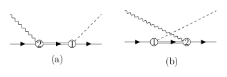
Figure 4: Feynman diagrams including the contribution of the $\Delta$ resonance to pion electroproduction. Numbers indicate the chiral order of the vertex.

The relevant Lagrangian terms are Hiller Blin et al. (2016); Pascalutsa (2008)

$$\mathcal{L}_{\Delta N\pi}^{(1)}=\frac{ih_{A}}{2Fm_{\Delta}}\bar{N}T^{a}\gamma^{\mu\nu\lambda}(\partial_{\mu}\Delta_{\nu})\partial_{\lambda}\pi^{a}+\text{h.c.},$$ (36)

$$\mathcal{L}_{\Delta N\gamma}^{(2)}=\frac{3ieg_{M}}{2m(m+m_{\Delta})}\bar{N}T^{3}(\partial_{\mu}\Delta_{\nu})\widetilde{f}^{\mu\nu}+\text{h.c.},$$ (37)

with $h_{A}$ that can be fixed from the strong $\Delta\rightarrow\pi N$ decay, and $g_{M}$ from the electromagnetic one, $\Delta\rightarrow\gamma N$. Also, $\gamma^{\mu\nu\lambda}=\frac{1}{4}\left\{\left[\gamma^{\mu},\gamma^{\nu}\right],\gamma^{\lambda}\right\}$ and $\widetilde{f}^{\mu\nu}=\frac{1}{2}\epsilon^{\mu\nu\alpha\beta}(\partial_{\alpha}A_{\beta}-\partial_{\beta}A_{\alpha})$. The $\Delta(1232)$ isospin multiplet is given by $\Delta_{\nu}=(\Delta^{++}_{\nu},\Delta^{+}_{\nu},\Delta^{0}_{\nu},\Delta^{-}_{\nu})^{T}$ and the isospin transition matrices $T^{a}$ can be found in Ref. Pascalutsa et al. (2007).

II.3.3 Isospin symmetry treatment

As it is obvious from our choice of the Lagrangian, the vertices are calculated in the isospin symmetric limit ($m_{u}=m_{d}$). However, the physical masses of pions and nucleons are used in the evaluation of the loops. Formally, in our $\mathcal{O}(p^{3})$ calculation, this amounts to a higher order correction. Nonetheless, it allows to properly reproduce the cusp, due to the different thresholds for the two charge channels, clearly visible in the $E_{0+}$ multipole for the $\gamma p\rightarrow\pi^{0}p$ reaction Bernard et al. (1994). In general, it should lead to some visible changes very close to threshold, where the isospin mass splittings could be relevant, while producing only small numerical changes at higher energies.

II.4 Low-energy-constants and fitting procedure

Table 1: Values of the LECs determined from other processes.

	LEC	Value	Source
$\mathcal{L}_{N}^{(2)}$	$\widetilde{c}_{6}$	$5.07\pm 0.15$	$\mu_{p}$ and $\mu_{n}$ Bauer et al. (2012); Yao et al. (2018); Tanabashi et al. (2018)
	$\widetilde{c}_{7}$	$-2.68\pm 0.08$	$\mu_{p}$ and $\mu_{n}$ Bauer et al. (2012); Yao et al. (2019); Tanabashi et al. (2018)
$\mathcal{L}_{N}^{(3)}$	$d_{6}$	$-0.70\;\text{GeV}^{-2}$	$N$ EM Form factor Fuchs et al. (2004)
	$d_{7}$	$-0.49\;\text{GeV}^{-2}$	$N$ EM Form factorFuchs et al. (2004)
	$d_{18}$	$-0.02\pm 0.08\;\text{GeV}^{-2}$	$\pi N$ scattering Alarcon et al. (2013)
$\mathcal{L}_{\pi\pi}^{(4)}$	$l_{6}$	$(-1.34\pm 0.12)\times 10^{-2}$	$\langle r^{2}\rangle_{\pi}$ Yao et al. (2018)
$\mathcal{L}_{\Delta N\pi}^{(1)}$	$h_{A}$	$2.87\pm 0.03$	$\Gamma_{\Delta}^{\rm strong}$ Bernard et al. (2013)
$\mathcal{L}_{\Delta N\gamma}^{(2)}$	$g_{M}$	$3.16\pm 0.16$	$\Gamma_{\Delta}^{\rm EM}$ Hiller Blin et al. (2015b)

Many of the LECs appearing in the Lagrangian have been obtained from the study of other processes or physical quantities. In the lowest order Lagrangian, $\mathcal{L}_{N}^{(1)}$, the chiral quantities $\widetilde{g}$, $F$, $\widetilde{m}$ and $M$ are expressed in terms of their corresponding physical values, see Appendix, Sec. V.5. For the leading order Lagrangian and the rest of physical quantities we take $F_{\pi}=92.42$ MeV, $g_{A}=1.27$, $m_{\Delta}=1232$ MeV and $e^{2}=4\pi/137$.

In this work, we compare our model with the experimental database and minimize the $\chi^{2}$, taking as fitting parameters the remaining free LECs. In particular, the combination $\{d_{8}+d_{9}\}$ that appears exclusively in the $\pi^{0}p$ channel, and the set $\{d_{9},d_{20},d_{21},d_{22}\}$ contributing to the charged pion channels, as shown in Appendix, Sec. V.2. In Ref. Guerrero Navarro et al. (2019), $d_{22}$, related to the nucleon axial radius, was fixed from a fit to lattice data at unphysical pion masses Yao et al. (2017). However, the quoted error bars might be underestimated  and we prefer to fix it independently. Furthermore, in the previous studies of pion photoproduction, its value could not be well assessed because, at $Q^{2}=0$, its contribution is fully correlated to that of $d_{21}$. Thus, the inclusion of electroproduction in the current analysis could lead to a more reliable determination of this parameter.

II.5 Estimation of the observable uncertainties

We consider two error sources in our calculation of the observables. One comes from the statistical error in the LECs due to the error bars in the experimental data. We propagate the error bars in the fitting LECs to an associated error, $\delta\mathcal{O}_{\text{LECs}}$, for any observable $\mathcal{O}$ through the relation,

$$\delta\mathcal{O}_{\text{LECs}}= \left(\sum_{i,j}\left[\text{Corr}(x_{i},x_{j})\right]\frac{\partial\mathcal{O}(\bar{x}_{i})}{\partial x_{i}}\delta x_{i}\frac{\partial\mathcal{O}(\bar{x}_{j})}{\partial x_{j}}\delta x_{j}\right)^{1/2},$$ (38)

where Corr$(x_{i},x_{j})$ indicates the $(i,j)$-th element of the correlation matrix, giving the estimated correlation among the $x_{i}$ and $x_{j}$ LECs. Moreover $\bar{x}_{i}$, $\delta{x}_{i}$ refers to the mean and the error values obtained from the fit for any LEC $x_{i}$.

In addition, another source of error is the systematical error of the theory due to the truncation of the chiral series expansion at a given $\mathcal{O}(p^{n})$. We use the method of Refs. Epelbaum et al. (2015); Siemens et al. (2016), namely, for an order $n$ calculation, $\mathcal{O}_{\text{Th}}^{(n)}$, we estimate this systematical error as

$$\delta\mathcal{O}_{\text{Th}}^{(n)}= \text{max}\left(\left|\mathcal{O}^{(n_{LO})}\right|B^{n-n_{LO}+1},\left\{\left|\mathcal{O}^{(k)}-\mathcal{O}^{(l)}\right|B^{n-l}\right\}\right),\hskip 28.45274ptn_{LO}\leq l\leq k\leq n.$$ (39)

We take $B=m_{\pi}/\Lambda_{b}$ and $\Lambda_{b}$ the breakdown scale of the chiral expansion, $\Lambda_{b}=4\pi F_{\pi}\sim 1$ GeV as in Ref. Yao et al. (2017). In the present work we have $n_{LO}=1$ as the lowest order and the upper order is $n=3$.

II.6 Experimental database

We compare our model to the available experimental data with some kinematical limits to ensure small external momenta while staying well below the $\Delta(1232)$ resonance peak. Thus, we have taken the invariant energy of the $\pi N$ system ranging from threshold up to $1130$ MeV. Furthermore, from the study of the nucleon electromagnetic form factors  Kubis and Meissner (2001); Bauer et al. (2012) it is known that a good description beyond $Q^{2}\sim 0.2$ GeV² requires the inclusion of vector mesons in the model. Therefore, we have selected data with transfer momentum, $Q^{2}<0.15$ GeV². In particular, the case for $Q^{2}=0$ corresponds to pion photoproduction. We expect the $\mathcal{O}(p^{3})$ ChPT calculation with explicit $\Delta$’s to be well suited for the description of the phenomenology in this kinematical region.

II.6.1 Electroproduction

The largest amount of data corresponds to the $\gamma^{*}p\rightarrow\pi^{0}p$ channel. Specifically, from the late nineties, we include data for the virtual angular cross section $d\sigma_{v}/d\Omega_{\pi}$ at $Q^{2}=0.1\;\text{GeV}^{2}$, obtained by the Amsterdam Pulse Stretcher facility van den Brink et al. (1997), and data from MAMI Distler et al. (1998) for the observables $d\sigma_{TT}/d\Omega_{\pi}$, $d\sigma_{TL}/d\Omega_{\pi}$ and the combination $\left(d\sigma_{T}/d\Omega_{\pi}+\varepsilon d\sigma_{L}/d\Omega_{\pi}\right)$. Later, very precise energy dependence data has been obtained at $Q^{2}=0.05\;\text{GeV}^{2}$ in Mainz Weis et al. (2008) for the observables $d\sigma_{TT}/d\Omega_{\pi}$, $d\sigma_{TL}/d\Omega_{\pi}$, $\left(d\sigma_{T}/d\Omega_{\pi}+\varepsilon d\sigma_{L}/d\Omega_{\pi}\right)$ and the asymmetry $A_{TLP^{\prime}}$. More recently, data for $d\sigma_{TL}/d\Omega_{\pi}$ and $\left(d\sigma_{T}/d\Omega_{\pi}+\varepsilon d\sigma_{L}/d\Omega_{\pi}\right)$ were published for additional $Q^{2}$ values Merkel et al. (2011).

There are far less data for the pion charged channel $\gamma^{*}p\rightarrow\pi^{+}n$. Nonetheless, they are crucial to determine LECs like $d_{20}$ and $d_{21}$. We consider data on $d\sigma_{T}/d\Omega_{\pi}$, $\sigma_{L}/d\Omega_{\pi}$, $d\sigma_{TL}/d\Omega_{\pi}$ and the total $d\sigma_{v}/d\Omega_{\pi}$ at a fixed $Q^{2}=0.117$ GeV² measured at Mainz Blomqvist et al. (1996). Later, the experiment was extended to other $Q^{2}$ values for $d\sigma_{T}/d\Omega_{\pi}$, $\sigma_{L}/d\Omega_{\pi}$ and $d\sigma_{v}/d\Omega_{\pi}$ Liesenfeld et al. (1999); Baumann (2005), and more recently to lower energies Friščić et al. (2017).

II.6.2 Photoproduction

We extend the database used in Ref. Guerrero Navarro et al. (2019) with the inclusion of some recent data. For the $\gamma p\rightarrow\pi^{0}p$ channel, we have added the measurements on transverse polarized protons from Ref. Schumann et al. (2015). They correspond to the observable $Td\sigma/d\Omega_{\pi}$ Schumann et al. (2015), where $T$ is the target asymmetry and $d\sigma/d\Omega_{\pi}$ the differential cross section Guerrero Navarro et al. (2019). We have also included the total cross section results for the threshold photoproduction on the neutron from Ref. Briscoe et al. (2020).

III Results and discussion

III.1 Low-Energy-Constants

The theoretical model has been compared with the full photoproduction and electroproduction database previously introduced, minimizing the $\chi$-squared function by varying the values of the free LECs. In the calculation, we have fixed the LECs from Table 1 to their central values, except for $g_{M}$. We have let the $\gamma\Delta N$ coupling, $g_{M}$, which proved of paramount significance in the description of $\pi^{0}$ photoproduction Hiller Blin et al. (2015a), to fluctuate around the central value obtained from the electromagnetic $\Delta$ width.

Table 2: Fit results for the LECs. The coupling $g_{M}$ is dimensionless and $d_{i}$ in units of GeV^-2.

	$d_{8}+d_{9}$	$d_{8}-d_{9}$	$d_{20}$	$d_{21}$	$d_{22}$	$g_{M}$	$\chi^{2}$	$\chi^{2}_{\gamma}$	$\chi^{2}_{e}$
Full model	$1.12\pm 0.01$	$0.63\pm 0.15$	$-0.29\pm 0.09$	$1.64\pm 0.06$	$0.95\pm 0.13$	$2.90\pm 0.01$	2.7	1.7	5.1
$\Delta$-less	$3.44\pm 0.01$	$4.75\pm 0.18$	$-3.01\pm 0.09$	$4.50\pm 0.06$	$0.45\pm 0.12$	-	13.2	16.8	4.4

We have chosen to fit the combinations $\{d_{8}+d_{9}\}$ and $\{d_{8}-d_{9}\}$, instead of the individual constants, because of the important correlation among $d_{8}$ and $d_{9}$. Actually, they appear in the amplitudes for $\pi^{0}$ production just in the combination $\{d_{8}+d_{9}\}$, while the charged $\pi^{\pm}$ channels depend only on $d_{9}$. Given that the $\pi^{0}$ processes represent, so far, the most precise and largest amount of data, the $\{d_{8}+d_{9}\}$ combination can be determined with a higher accuracy. Evidently, better data for the $\pi^{\pm}$ channels, would be essential to obtain more precise results for $d_{9}$ or, similarly, for $\{d_{8}-d_{9}\}$.

The parameters $\{d_{20},d_{21},d_{22}\}$ are only relevant for the charged channels $\gamma(^{*})p\rightarrow\pi^{+}n$ and $\gamma(^{*})n\rightarrow\pi^{-}p$. The relatively low precision of the data and their scarcity limits the precision of their determination. Furthermore, these channels are already rather well described by the lower order predictions and in consequence the $\mathcal{O}(p^{3})$ LECs play a small role. It is worth mentioning that in photoproduction, $d_{21}$ and $d_{22}$ appear only in the combination $\{2d_{21}-d_{22}\}$ while for electroproduction that is not anymore the case (see App. Sec. V.2). Therefore, the full correlation is broken once electroproduction is considered in the fit.

Clearly, pion electroproduction reactions probe the $Q^{2}$ dependence of the scattering amplitude. Thus, it allows for the exploration of LECs like $\{d_{6},d_{7},l_{6}\}$, which are relevant for the description of the nucleon EM form factors and the pion charge radius and which appear in the electroproduction case.

The LECs values obtained by the fit are presented in Table 2, together with the full $\chi^{2}$ per degree of freedom and the partial contributions of photo-($\chi^{2}_{\gamma}$) and electroproduction ($\chi^{2}_{e}$). All the fitted $d_{i}$’s are of natural size and, thus, the contribution of the associated mechanisms is relatively small at low energies. While the global result is acceptable, as it will be better shown in the detailed comparison with various observables, it is clear that the model reproduces to a greater degree the photoproduction data.

The results for $g_{M}$ and $\{d_{8}+d_{9}\}$ agree well with those obtained in the analysis of Ref. Guerrero Navarro et al. (2019), which studied photoproduction within the same framework but imposed full isospin symmetry on the loop calculation. Our change, using physical masses in the loops, has led to a substantially lower $\chi^{2}_{\gamma}$ value and to some small changes in $\{d_{8}-d_{9}\}$ and $d_{20}$. A larger variation can be observed in $d_{21}$ and $d_{22}$ but this could be deceptive. The photoproduction amplitude only depends on the combination $\{2d_{21}-d_{22}\}$, which it has changed little. The separation of the two constants made in Ref. Guerrero Navarro et al. (2019) was based on the use of $d_{22}=5.20\;\text{GeV}^{-2}$, taken from Ref. Yao et al. (2017). This value, obtained from lattice and already discussed, is clearly disfavoured by the electroproduction data. However, our result is close to an alternative fit of Ref. Yao et al. (2017) that restricted lattice data to low $Q^{2}$ values.

All the fitted $d_{i}$’s appear in the evaluation of neutrino induced pion production off nucleons and could be used to improve the corresponding predictions. This is specially important in the current precision era of neutrino physics, where an adequate modelling of cross sections and backgrounds is necessary for the investigation of neutrino masses, mixing angles and other properties Alvarez-Ruso et al. (2014). Our results give support to the first ChPT calculations of these weak production processes Yao et al. (2018, 2019), which assumed a natural size for these parameters to estimate the uncertainties of the theoretical predictions.

III.2 Electroproduction observables

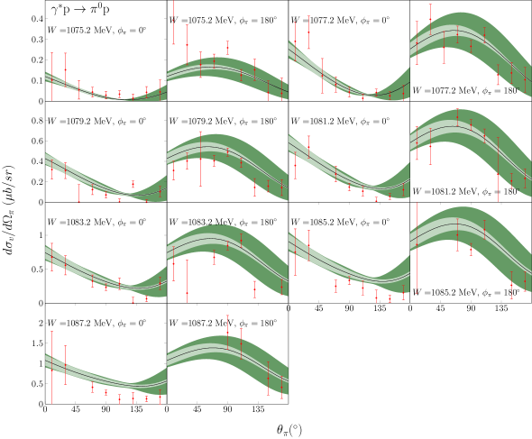
Figure 5: Angular distribution of the virtual cross section $d\sigma_{v}/d\Omega_{\pi}$ at different angles and energies, transfer momentum $Q^{2}=0.10\;\text{GeV}^{2}$ and virtual-photon polarization $\varepsilon=0.670$. Solid line shows the theoretical results, the inner band depicts the statistical error from the LECs variation within 1-$\sigma$ as in Table 2. The outer band represents the total error including the systematical error from chiral truncation, Eq. (39), added to the statistical one in quadrature. Data from Ref. van den Brink et al. (1997).

Figure 6: $d\sigma_{TT}/d\Omega_{\pi}$ and $d\sigma_{TL}/d\Omega_{\pi}$ as function of the c.m. pion angle $\theta_{\pi}$ for the channel $\gamma^{*}p\rightarrow\pi^{0}p$ at $Q^{2}=0.1\;\text{GeV}^{2}$ and with polarization $\varepsilon=0.713$. Data from Ref. Distler et al. (1998). Description as in Fig. 5.

III.2.1 $\gamma^{*}p\rightarrow\pi^{0}p$ channel

In this section, we show our results for the $\pi$ electroproduction process compared to the experimental data. We start with the $\gamma^{*}p\rightarrow\pi^{0}p$ channel, that represents the largest amount of data, in Figs. 5-8. We should remark that, among the third order fitted LECs, this channel’s amplitude depends only on the $\{d_{8}+d_{9}\}$ combination, that is much constrained by neutral pion photoproduction. Actually, the current fit results for that LEC are fully consistent with the previous determination based just on photoproduction Guerrero Navarro et al. (2019). Overall, the agreement with data is good for all the observables considered here.

In Fig. 5, we show the virtual photon cross section, $d\sigma_{v}/d\Omega_{\pi}$, at several energy bins close to threshold, $Q^{2}=0.10\;\text{GeV}^{2}$ and for $\varepsilon=0.67$, compared to the NIKHEF data from Ref. van den Brink et al. (1997). The angular dependence, on both $\theta_{\pi}$ and $\phi_{\pi}$, and the energy dependence are well reproduced.

The various pieces, related to the longitudinal and transverse responses and their interference, which contribute to the total cross section of Eq. (13), are explored next. In Fig. 6, we compare the model with the angular dependence of $\sigma_{TT}$ and $\sigma_{TL}$ measured by MAMI Distler et al. (1998) at several energies very close to threshold. The two observables are very small. Both the size and the energy dependence are well accounted for by our calculation. Much larger is the observable $d\sigma_{T}/d\Omega_{\pi}+\varepsilon d\sigma_{L}/d\Omega_{\pi}$ from a much more recent MAMI experiment Merkel et al. (2011) and depicted in Fig. 7. These latter results show the $Q^{2}$ dependence, that at the low energies involved and for the relatively small $Q^{2}$ values is well described by the model.

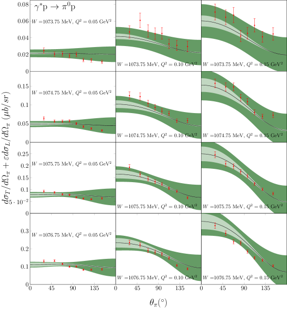
Figure 7: Angular distribution for $d\sigma_{T}+\varepsilon d\sigma_{L}$ at different c.m. energy values, $W$. The transfer momenta at $Q^{2}=0.05\;\text{GeV}^{2}$ corresponds to polarization values of $\varepsilon=0.932$, $Q^{2}=0.10\;\text{GeV}^{2}$ to $\varepsilon=0.882$ and $Q^{2}=0.15\;\text{GeV}^{2}$ to $\varepsilon=0.829$. Data from Merkel et al. (2011) and description as in Fig.5.

The $Q^{2}$ dependence is also explored for $d\sigma_{TL}$ in Fig. 8, which also shows a good agreement for the angular distribution at several $Q^{2}$ values. We should remark that for neutral pions, apart from the fixed LECs, this dependence is only sensitive to $\{d_{8}+d_{9}\}$ and $g_{M}$, which are strongly constrained by the photoproduction ($Q^{2}=0$) data.

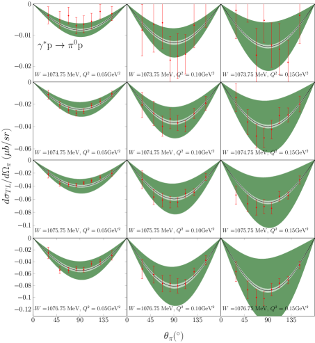
Figure 8: Angular distribution for $d\sigma_{TL}/d\Omega_{\pi}$ for different c.m. energy values, W. The transfer momenta at $Q^{2}=0.05\;\text{GeV}^{2}$ corresponds to polarization values of $\varepsilon=0.932$, $Q^{2}=0.10\;\text{GeV}^{2}$ to $\varepsilon=0.882$ and $Q^{2}=0.15\;\text{GeV}^{2}$ to $\varepsilon=0.829$. Data from Merkel et al. (2011) and description as in Fig. 5.

Finally, in Fig. 9, we compare our calculation with the very copious and precise data of Ref. Weis et al. (2008), where the energy dependence of $d\sigma_{T}$, $d\sigma_{TT}$, $d\sigma_{TL}$ and $A_{LT^{\prime}}$ has been investigated at $Q^{2}=0.05\;\text{GeV}^{2}$ and photon transverse polarization $\varepsilon=0.933$. For $d\sigma_{T}/d\Omega_{\pi}+\varepsilon d\sigma_{L}/d\Omega_{\pi}$ and $d\sigma_{TT}/d\Omega_{\pi}$, the calculation agrees well up to a few MeV above threshold, what is consistent with the results shown in Fig. 7. However, we overestimate the absolute value of the observable at higher energies. In fact, our fit curve behaves as the HBChPT result of Ref. Bernard et al. (1996d) discussed in Weis et al. (2008). The agreement with $\sigma_{TT}$ is good and with $\sigma_{TL}$ excellent, in both cases improving the HBChPT prediction. In these three cases, the quality of the agreement of our $\mathcal{O}(p^{3})$ model is very similar to that of the $\mathcal{O}(p^{4})$ $\Delta$-less covariant ChPT calculation of Ref. Hilt et al. (2013a).

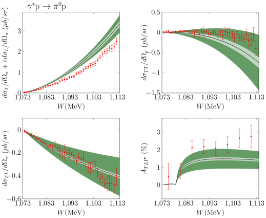
Figure 9: Energy dependence for $d\sigma_{T}+\varepsilon d\sigma_{L}$, $d\sigma_{TT}$, $d\sigma_{TL}$ and $A_{LT^{\prime}}$ at $Q^{2}=0.05\;\text{GeV}^{2}$, $\varepsilon=0.933$, $\theta_{\pi}=90^{\circ}$. Data from Weis et al. (2008).

Also well reproduced is the beam helicity asymmetry, $A_{LT^{\prime}}$, a quite small effect, which shows the cusp related to the $n\pi^{+}$ threshold. The use of the physical masses in the loops, and the corresponding isospin symmetry breaking is essential for a proper reproduction of this shape.

Summarizing, the theoretical results for the $\pi^{0}$ channel are in accordance with data, describing properly the angular dependence and the $Q^{2}$ evolution. In regard to the energy, we obtain the best results very close to threshold. Nonetheless, the model starts to overestimate data for the observable $d\sigma_{T}+\varepsilon d\sigma_{L}$ at higher energies, see Fig. 9. Actually, this observable contributes strongly to the total $\chi^{2}$. On the other hand, it is very sensitive to $c_{6}+c_{7}$, $2d_{7}+d_{6}$ and $g_{M}$, which were restricted to the values allowed by the study of other processes. In our calculation, the only totally free parameter relevant for this channel has been the combination $\{d_{8}+d_{9}\}$, strongly constrained by the abundant photoproduction data.

III.2.2 $\gamma^{*}p\rightarrow\pi^{+}n$ channel

The channel $\gamma^{*}p\rightarrow\pi^{+}n$ depends on the $\mathcal{O}(p^{3})$ LECs $d_{9}$, $d_{20}$, $d_{21}$ and $d_{22}$, as well as the $\mathcal{O}(p^{4})$ one $l_{6}$. Thus, there are more fitting LECs than for the neutral pion channel. Furthermore, the data are scarce. For these reasons, there are less constrains on the relevant LECs and the statistical error is considerably wider.

We find that the few and scattered virtual photon cross section data Blomqvist et al. (1996); Liesenfeld et al. (1999) agree well, within errors, with the theoretical model, and that the $\pi^{+}$ channel is more sensitive to the lower orders than to the $\mathcal{O}(p^{3})$ contributions. In Fig. 10, we present $d\sigma_{T}$, $d\sigma_{L}$ and $d\sigma_{TL}$ as a function of $Q^{2}$ at various pion angles and from several experiments that are also well reproduced.

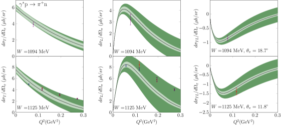
Figure 10: $d\sigma_{T}$, $d\sigma_{L}$ and $d\sigma_{TL}$ as functions of $Q^{2}$ for the $\gamma^{*}p\rightarrow\pi^{+}n$ process. For $d\sigma_{T}$ and $d\sigma_{L}$, the pion angle is $\theta_{\pi}=0^{\circ}$. Magenta circles: data from Friščić et al. (2017). Red squares: data from Blomqvist et al. (1996); Liesenfeld et al. (1999). Blue dots: data from Baumann (2005).

III.3 Photoproduction

The use of physical masses in the loop propagators and, therefore, the breaking of the isospin symmetry is the main difference of this calculation with Refs. Hiller Blin et al. (2016); Guerrero Navarro et al. (2019). It leads to a better description of the low energy region, where the effects of the different masses and thresholds are more relevant. Furthermore, in Refs. Hiller Blin et al. (2016); Guerrero Navarro et al. (2019), there was a systematic overestimation of the cross section at backward angles for the $\pi^{0}p$ channel at all energies. The breaking of the isospin symmetry in the loops has now much improved the agreement with that cross section. As a consequence, the partial $\chi^{2}$, considering only photoproduction, has been reduced from 3.2 to 1.5. Also, without isospin breaking, the fit prefers values of $d_{18}$ large and positive, which are inconsistent with $\pi N$ scattering. Now, the tension is much reduced and the $\chi^{2}$ depends less strongly on that parameter. In the following, we present our results putting emphasis on the comparison with the new data, added to the database after Ref. Guerrero Navarro et al. (2019), and in the low energy region, that had not been included in the previous fit.

The $\gamma p\rightarrow\pi^{0}p$ channel is the most richly represented in the database, both in the amount and the precision of data. Thus, the relevant LECs, in particular the $d_{8}+d_{9}$ combination, are strongly constrained and get a relatively small uncertainty in the fit.

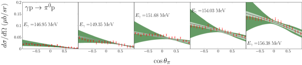
Figure 11: Angular cross section for the channel $\gamma p\rightarrow\pi^{0}p$. Data from Ref. Hornidge et al. (2013).

In Fig. 11, we show the near threshold region for the angular distribution and in Fig. 12 the integrated total cross section $\sigma$ as function of the energy.

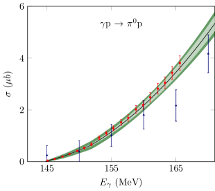
Figure 12: Cross section close to threshold for $\gamma p\rightarrow\pi^{0}p$. Red circles: data from Ref. Schmidt et al. (2001), blue triangles: data from Ref. Schumann et al. (2010), not included in the fit.

Both are well reproduced. Our calculation still preserves the excellent results for the energy dependence of the total cross section and for the beam asymmetry as in the previous work Guerrero Navarro et al. (2019).

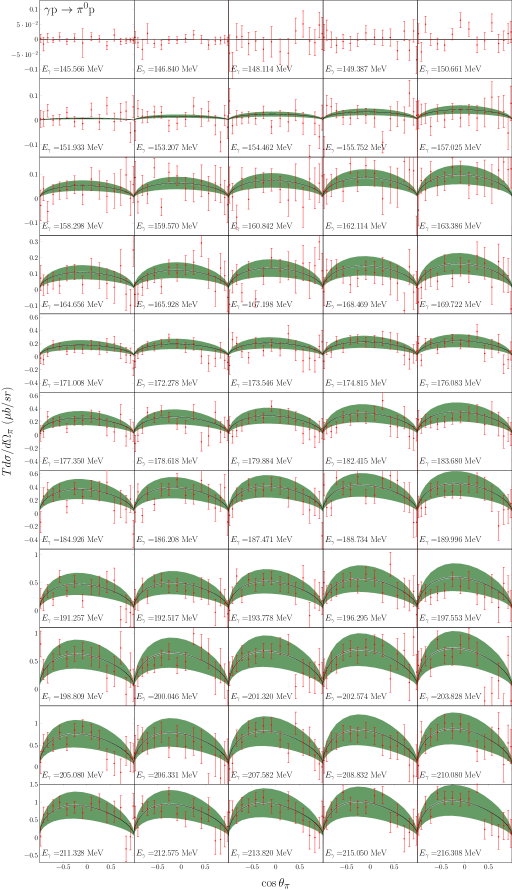
Figure 13: Angular distribution of $Td\sigma/d\Omega_{\pi}$ for the $\gamma p\rightarrow\pi^{0}p$ channel. Data from Schumann et al. (2015).

In addition, for the $\pi^{0}p$ channel, we have analyzed the data from Ref. Schumann et al. (2015) studying the process occurring on transversely polarized protons. The observable $Td\sigma/d\Omega_{\pi}$ is sensitive to the cusp effects due to the $n\pi^{+}$ threshold. The results are shown in Fig. 13, with $T$ and present a good agreement for the full range of energies.

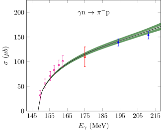
Figure 14: Cross section for the $\gamma n\rightarrow\pi^{-}p$ process. Data from Briscoe et al. (2020) in magenta circles; red squares, data from White et al. (1960) and blue dots, data from Wang (1992) (not included in the fit).

The quality of the agreement with the channels with charged pions has also improved upon Ref. Guerrero Navarro et al. (2019), as can be seen comparing the partial $\chi^{2}$’s. We would like to emphasize the recent results, shown in Fig. 14, for the $\gamma n\rightarrow\pi^{-}p$ process Briscoe et al. (2020) very close to threshold. They have considerably enriched the database for this channel and therefore lead to a better determination of the LECs relevant for this channel, $d_{9}$, $d_{20}$ and the combination $2d_{21}-d_{22}$.

III.4 $\Delta$ contribution

To explore the importance of the inclusion of the explicit $\Delta(1232)$ in the model, we repeated the fit without the corresponding mechanisms. The results for the LECs and $\chi^{2}$ are shown in the second row of Table 2. It is remarkable that the $\Delta$ contribution, which depends only on well constrained parameters, ($h_{A}$ and $g_{M}$), improves substantially the global agreement with data. It is also noteworthy that most of the fitted $d_{i}$ LECs are much larger in the $\Delta$-less case, indicating the need of a more important third order and a slower chiral convergence. Comparing with the full model, we see that, with the current data set, the $\chi^{2}$ for photoproduction is considerably worsened, whereas for electroproduction $\chi^{2}$ is little modified, even showing a little improvement. In particular, we have found that $\Delta$ inclusion worsens the overestimation for $d\sigma_{T}/d\Omega_{\pi}$ in Fig. 9. However, it improves the agreement with the other observables of the same figure. This point is relevant, because that observable has the largest, may be excessive, weight in the $\chi^{2}$ calculation among the full electroproduction data set, followed by $d\sigma_{TT}/d\Omega_{\pi}$ from the same experiment Weis et al. (2008). This is due to the large number of points and their precision.

In contrast, the $\Delta$ role in photoproduction is of the uttermost importance to reproduce the energy dependence of data. The $\Delta$-less model is unable to describe the energy evolution of the cross sections, mostly in the $\pi^{0}$ channel, even with the inclusion of the $\mathcal{O}(p^{3})$ one-loop amplitudes. This failure can be appreciated in Fig. 15. There, we show the $\chi^{2}$ per degree of freedom as a function of the maximum invariant energy, $W$ considered in the fitting procedure. The quality of the agreement remains stable for the full model whereas without explicit $\Delta$ the $\chi^{2}$ function grows fast as a function of the energy and it is impossible to describe data at this chiral order.

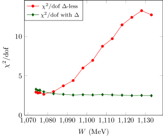
Figure 15: $\chi^{2}/$dof as function of the maximum $W$ considered in the fitting procedure. Full model at $\mathcal{O}(p^{3})$ with $\Delta$ (green diamonds) and without $\Delta$ (red circles).

IV Summary

In this work, we have studied pion production off the nucleon induced by virtual and real photons at low energies. We have made a full $\mathcal{O}(p^{3})$ calculation, in the $\delta$ counting, in covariant ChPT including explicitly the $\Delta(1232)$ resonance and employing the EOMS renormalization scheme. The free LECs of the theoretical model have been fixed by fitting it to the available pion electro- and photoproduction data. We have considered a restricted kinematical region with $\sqrt{s}<1.13$ GeV and $Q^{2}<0.15$ GeV², where we expect our model to be reliable and still well below the $\Delta(1232)$ peak.

We have confirmed the importance of the loop terms. The imaginary parts of the scattering amplitude and the cusp effects, coming from the opening of the various charge channels, are crucial in the description of some low energy observables. To properly account for these effects we have used the physical masses of mesons and baryons in the evaluation of the loops, therefore breaking isospin symmetry.

The model describes well all data for total cross section, angular distributions and numerous polarization observables. In particular, the agreement is excellent for photoproduction data. In fact, it is better than for other higher order chiral calculations Fernandez-Ramirez and Bernstein (2013); Hilt et al. (2013a) that do not include the $\Delta$ resonance. Without $\Delta$, our model is only able to reproduce data a few MeV above threshold. Neutral pion photoproduction is the most sensitive channel to this resonance due to the smallness of the lower order contributions.

The comprehensive investigation of all electro- and photoproduction channels, including all the available observables, has allowed to disentangle all the relevant third order LECs involved, $\{d_{8},d_{9},d_{20},d_{21},d_{22}\}$. The values obtained for the fitted LECs are all of natural size, what is satisfactory from the point of view of chiral convergence. Furthermore, this gives support to the uncertainty estimations of recent chiral calculations of neutrino induced pion production. Our results will allow for more precise predictions of the low energy neutrino nucleon cross sections of relevance to achieve the precision goals of modern neutrino experiments.

V Appendix

V.1 Amplitude parametrizations

The electromagnetic matrix element between the hadronic states, $\mathcal{M}^{\mu}$, can be written in terms of the Ball amplitudes Ball (1961),

$$\mathcal{M}^{\mu}=\bar{u}(p^{\prime},s^{\prime})\left(\sum_{i=1}^{8}b_{i}V_{i}^{\mu}\right)u(p,s)$$ (40)

with the Ball vector basis, see e.g. Hilt et al. (2013a),

$$\begin{split}V_{1}^{\mu}=\gamma^{\mu}\gamma^{5},\;\;&V_{2}^{\mu}=P^{\mu}\gamma^{5},\\ V_{3}^{\mu}=q^{\mu}\gamma^{5},\;\;&V_{4}^{\mu}=k^{\mu}\gamma^{5},\\ V_{5}^{\mu}=\gamma^{\mu}\not{k}\gamma^{5},\;\;&V_{6}^{\mu}=P^{\mu}\not{k}\gamma^{5},\\ V_{7}^{\mu}=q^{\mu}\not{k}\gamma^{5},\;\;&V_{8}^{\mu}=k^{\mu}\not{k}\gamma^{5},\end{split}$$ (41)

where $P^{\mu}=(p+p^{\prime})^{\mu}/2$. As the current $J^{\mu}$, from Eq. 2, obeys the continuity equation, we also have $k_{\mu}\mathcal{M}^{\mu}=0$, leading us to the following relations,

$$\begin{split}b_{1}=&-b_{6}(k\cdot P)-b_{7}(k\cdot q)+b_{8}Q^{2},\\ b_{2}=&\frac{1}{k\cdot P}\left(Q^{2}(b_{4}+b_{5})-b_{3}(k\cdot q)\right).\end{split}$$ (42)

These relations are sufficient to impose the gauge invariance in the scattering amplitude. They also reduce from eight to six the independent elements of the basis $\{V_{i}\}$. Another common parametrization, in terms of the covariant basis elements $M_{i}^{\mu}$, is Drechsel and Tiator (1992)

$$\sum_{i=3}^{8}b_{i}V_{i}^{\mu}=\sum_{j=1}^{6}A_{j}M_{j}^{\mu}\,,$$ (43)

where

$$\begin{split}M_{1}^{\mu}=&-\frac{i}{2}\gamma^{5}\left(\gamma^{\mu}\not{k}-\not{k}\gamma^{\mu}\right),\\ M_{2}^{\mu}=&2i\gamma^{5}\left(P^{\mu}k\cdot\left(q-\frac{1}{2}k\right)-\left(q-\frac{1}{2}k\right)^{\mu}k\cdot P\right),\\ M_{3}^{\mu}=&-i\gamma^{5}\left(\gamma^{\mu}(k\cdot q)-q^{\mu}\not{k}\right),\\ M_{4}^{\mu}=&im_{N}\gamma^{5}(\gamma^{\mu}\not{k}-\not{k}\gamma^{\mu})-2i\gamma^{5}(\gamma^{\mu}k\cdot P-P^{\mu}\not{k}),\\ M_{5}^{\mu}=&i\gamma^{5}\left(k^{\mu}(k\cdot q)+Q^{2}q^{\mu}\right),\\ M_{6}^{\mu}=&-i\gamma^{5}\left(k^{\mu}\not{k}+Q^{2}\gamma^{\mu}\right)\,.\end{split}$$ (44)

In the case of photoproduction, $Q^{2}=0$, and then $\epsilon_{\mu}M_{j}^{\mu}=0$ for $j=5,6$.

The relations among the above mentioned parametrizations are given by

$$\begin{split}A_{1}=&i(b_{5}+b_{6}m_{N}),\\ A_{2}=&-\frac{i\left(-b_{3}(k\cdot q)+(b_{4}+b_{5})Q^{2}\right)}{(k\cdot P)(2k\cdot q+Q^{2})},\\ A_{3}=&ib_{7},\\ A_{4}=&\frac{ib_{6}}{2},\\ A_{5}=&-\frac{i(b_{3}+2(b_{4}+b_{5}))}{2k\cdot q+Q^{2}},\\ A_{6}=&-ib_{8}\,.\end{split}$$ (45)

Using the CGLN basis, as in Chew et al. (1957); Dennery (1961), we can write

$$\epsilon_{\mu}\mathcal{M}^{\mu}=\epsilon_{\mu}\bar{u}(p_{f})\left(\sum_{i=1}^{6}A_{i}M_{i}^{\mu}\right)u(p_{i})=4\pi\dfrac{W}{m_{N}}\chi_{f}^{\dagger}\mathcal{F}\chi_{i}\,.$$ (46)

Then, we find, expressed in the CM frame, the relations between the coefficients of both parametrizations as

$$\mathcal{F}_{1} = \frac{W-m_{N}}{8\pi W}\sqrt{E_{p}+m_{N}}\sqrt{E_{p^{\prime}}+m_{N}}\left(A_{1}+(W-m_{N})A_{4}-\frac{2m_{N}\nu_{B}}{W-m_{N}}(A_{3}-A_{4})+\frac{Q^{2}}{W-m_{N}}A_{6}\right),$$ (47)

$$\mathcal{F}_{2} = \frac{W+m_{N}}{8\pi W}|\vec{q}|\sqrt{\frac{E_{p}-m_{N}}{E_{p^{\prime}}+m_{N}}}\left(-A_{1}+(W+m_{N})A_{4}-\frac{2m_{N}\nu_{B}}{W+m_{N}}(A_{3}-A_{4})+\frac{Q^{2}}{W+m_{N}}A_{6}\right),$$ (48)

$$\mathcal{F}_{3} = \frac{W+m_{N}}{8\pi W}|\vec{q}|\sqrt{E_{p}-m_{N}}\sqrt{E_{p^{\prime}}+m_{N}}\left(\frac{2W^{2}-2m_{N}^{2}+Q^{2}}{2(W+m_{N})}A_{2}+A_{3}-A_{4}-\frac{Q^{2}}{W+m_{N}}A_{5}\right),$$ (49)

$$\mathcal{F}_{4} = \frac{W-m_{N}}{8\pi W}|\vec{q}|^{2}\sqrt{\frac{E_{p}+m_{N}}{E_{p^{\prime}}+m_{N}}}\left(-\frac{2W^{2}-2m_{N}^{2}+Q^{2}}{2(W-m_{N})}A_{2}+A_{3}-A_{4}+\frac{Q^{2}}{W-m_{N}}A_{5}\right),$$ (50)

$$\mathcal{F}_{5} = \frac{E_{\gamma}}{8\pi W}\sqrt{\frac{E_{p^{\prime}}+m_{N}}{E_{p}+m_{N}}}\mbox{\Huge{ $\{$ }}[E_{p}+m_{N}]A_{1}$$ (51)

$$+\left[4m_{N}\nu_{B}\left(W-\frac{3}{4}E_{\gamma}\right)-|\vec{p}_{\gamma}|^{2}W+E_{\pi}\left(W^{2}-m_{N}^{2}+\frac{1}{2}Q^{2}\right)\right]A_{2}$$

$$+[E_{\pi}(W+m_{N})+2m_{N}\nu_{B}]A_{3}$$

$$+[(E_{p}+m_{N})(W-m_{N})-E_{\pi}(W+m_{N})-2m_{N}\nu_{B}]A_{4}$$

$$+\left[2m_{N}\nu_{B}E_{\gamma}-E_{\pi}Q^{2}\right]A_{5}-[(E_{p}+m_{N})(W-m_{N})]A_{6}\mbox{\Huge{ $\}$ }},$$

$$\mathcal{F}_{6} = \frac{E_{\gamma}}{8\pi W}\frac{|\vec{q}|}{\sqrt{(E_{p^{\prime}}+m_{N})(E_{p}-m_{N})}}\mbox{\Huge{ $\{$ }}-[Ep-m_{N}]A_{1}$$ (52)

$$+\left[|\vec{p}_{\gamma}|^{2}W-4m_{N}\nu_{B}\left(W-\frac{3}{4}E_{\gamma}\right)-E_{\pi}\left(W^{2}-m_{N}^{2}+\frac{1}{2}Q^{2}\right)\right]A_{2}$$

$$+\left[E_{\pi}(W-m_{N})+2m_{N}\nu_{B}\right]A_{3}$$

$$+\left[(E_{p}-m_{N})(W+m_{N})-E_{\pi}(W-m_{N})-2m_{N}\nu_{B}\right]A_{4}$$

$$+\left[E_{\pi}Q^{2}-2m_{N}\nu_{B}E_{\gamma}\right]A_{5}-[(E_{p}-m_{N})(W+m_{N})]A_{6}\mbox{\Huge{ $\}$ }},$$

where $\nu_{B}=-\dfrac{k\cdot q}{2m_{N}}=-\dfrac{s+u-2m_{N}^{2}}{4m_{N}}$. Some care is needed here because different conventions for these functions can be found in the literature.

V.2 Amplitude pieces

V.2.1 $\mathcal{O}(q^{1})$ order

$$\mathcal{M}^{\mu\;(1)}_{(a)} =C_{I}^{(1)}\frac{eg}{F}V_{1}^{\mu},$$ (53)

$$\mathcal{M}^{\mu\;(1)}_{(b)} =C_{II}^{(1)}\frac{eg}{F}\left(\frac{\left(m_{N}^{2}-s\right)V_{1}^{\mu}}{s-m_{2}^{2}}-\frac{\left(m_{N}+m_{2}\right)\left(2V_{2}^{\mu}+V_{3}^{\mu}+V_{4}^{\mu}-V_{5}^{\mu}\right)}{m_{2}^{2}-s}\right),$$ (54)

$$\mathcal{M}^{\mu\;(1)}_{(c)} =C_{III}^{(1)}\frac{eg}{F}\left(\frac{\left(u-m_{N}^{2}\right)V_{1}^{\mu}}{u-m_{2}^{2}}-\frac{\left(m_{N}+m_{2}\right)\left(2V_{2}^{\mu}-V_{3}^{\mu}+V_{4}^{\mu}-V_{5}^{\mu}\right)}{m_{2}^{2}-u}\right),$$ (55)

$$\mathcal{M}^{\mu\;(1)}_{(d)} =C_{IV}^{(1)}\frac{\sqrt{2}em_{N}g\left(2V_{3}^{\mu}-V_{4}^{\mu}\right)}{F\left(-2m_{N}^{2}+Q^{2}+s+u\right)}.$$ (56)

The constants $C_{I}^{(1)},\dots,C_{IV}^{(1)}$ are given in Table 3 for each reaction channel. The amplitudes $\mathcal{M}^{\mu\;(1)}_{(b)}$ and $\mathcal{M}^{\mu\;(1)}_{(c)}$ are actually a combination of $\mathcal{O}(q^{1})$ and $\mathcal{O}(q^{2})$ orders due to the insertion of the nucleon mass at $\mathcal{O}(q^{2})$, $m_{2}$, in the $N$-propagator. This automatically generates the above diagrams at $\mathcal{O}(q^{1})$ with the chiral nucleon mass, $m$, in the propagator and the diagrams at $\mathcal{O}(q^{2})$ with the insertion of a vertex proportional to $c_{1}$ in the $N$-propagator, plus higher order small terms. As always, for the external legs we use physical masses.

Channel	$C_{I}^{(1)}$	$C_{II}^{(1)}$	$C_{III}^{(1)}$	$C_{IV}^{(1)}$
$\gamma^{*}p\rightarrow p\pi^{0}$	$0$	$\frac{1}{2}$	$\frac{1}{2}$	$0$
$\gamma^{*}p\rightarrow n\pi^{+}$	$\frac{1}{\sqrt{2}}$	$\frac{1}{\sqrt{2}}$	$0$	$-1$
$\gamma^{*}n\rightarrow p\pi^{-}$	$-\frac{1}{\sqrt{2}}$	$0$	$\frac{1}{\sqrt{2}}$	$1$
$\gamma^{*}n\rightarrow n\pi^{0}$	$0$	$0$	$0$	$0$

Table 3: Tree level amplitude constants for each channel at $\mathcal{O}(q^{1})$.

V.2.2 $\mathcal{O}(q^{2})$ order

$$\mathcal{M}^{\mu\;(2)}_{(b)} =C_{II}^{(2)}\frac{eg_{A}}{F_{\pi}}\left(-\frac{2V_{6}^{\mu}+V_{7}^{\mu}}{m_{N}^{2}-s}-\frac{\left(3m_{N}^{2}+s\right)\left(V_{4}^{\mu}-V_{5}^{\mu}\right)}{2m_{N}(m_{N}^{2}-s)}-V_{1}^{\mu}\right),$$ (57)

$$\mathcal{M}^{\mu\;(2)}_{(c)} =C_{III}^{(2)}\frac{eg_{A}}{F_{\pi}}\left(\frac{V_{7}^{\mu}-2V_{6}^{\mu}}{m_{N}^{2}-u}-\frac{\left(3m_{N}^{2}+u\right)(V_{4}^{\mu}-V_{5}^{\mu})}{2m_{N}(m_{N}^{2}-u)}+V_{1}^{\mu}\right).$$ (58)

The constants $C_{II}^{(2)}$ and $C_{III}^{(2)}$ are given in Table 4.

Channel	$C_{I}^{(2)}$	$C_{II}^{(2)}$	$C_{III}^{(2)}$	$C_{IV}^{(2)}$
$\gamma p\rightarrow p\pi^{0}$	$0$	$\frac{1}{2}(c_{6}+c_{7})$	$\frac{1}{2}(c_{6}+c_{7})$	$0$
$\gamma p\rightarrow n\pi^{+}$	$0$	$\frac{1}{\sqrt{2}}(c_{6}+c_{7})$	$\frac{1}{\sqrt{2}}c_{7}$	$0$
$\gamma n\rightarrow p\pi^{-}$	$0$	$\frac{1}{\sqrt{2}}c_{7}$	$\frac{1}{\sqrt{2}}(c_{6}+c_{7})$	$0$
$\gamma n\rightarrow n\pi^{0}$	$0$	$-\frac{1}{2}c_{7}$	$-\frac{1}{2}c_{7}$	$0$

Table 4: Tree level amplitude constants for each channel at $\mathcal{O}(q^{2})$.

V.2.3 $\mathcal{O}(q^{5/2})$ order

$$\begin{split}\mathcal{M}^{\mu\;(5/2)}_{(b)}=D_{II}&\frac{eh_{A}g_{M}}{24F_{\pi}m_{N}m_{\Delta}\left(m_{\Delta}+m_{N}\right)\left(m_{\Delta}^{2}-s-i\Gamma_{\Delta}m_{\Delta}\right)}\Biggl{[}\\ &\left\{m_{N}\left(m_{N}^{4}+m_{N}^{2}\left(-M_{\pi}^{2}+Q^{2}+2s\right)+M_{\pi}^{2}\left(s-Q^{2}\right)+s\left(-Q^{2}+3s-6u\right)\right)\right.\\ &\left.-m_{\Delta}\left(3m_{N}^{4}+m_{N}^{2}\left(M_{\pi}^{2}-Q^{2}-10s\right)+M_{\pi}^{2}\left(5Q^{2}-s\right)+s\left(Q^{2}+s+6u\right)\right)\right\}V_{1}^{\mu}\\ +&\left\{2Q^{2}\left(m_{N}^{2}-4m_{N}m_{\Delta}-M_{\pi}^{2}-5s\right)+6\left(m_{N}m_{\Delta}+s\right)\left(2m_{N}^{2}-s-u\right)\right\}V_{2}^{\mu}\\ +&\left\{Q^{2}\left(m_{N}^{2}-10m_{N}m_{\Delta}-M_{\pi}^{2}+s\right)+3(s-u)\left(m_{N}m_{\Delta}+s\right)\right\}V_{3}^{\mu}\\ +&\left\{Q^{2}\left(m_{N}^{2}-4m_{N}m_{\Delta}-M_{\pi}^{2}-5s\right)+m_{N}m_{\Delta}\left(2m_{N}^{2}+4M_{\pi}^{2}-3(5s+u)\right)\right.\\ &\left.-s\left(6m_{N}^{2}-4M_{\pi}^{2}+7s+3u\right)\right\}V_{4}^{\mu}\\ +&\left\{-m_{N}^{4}+m_{\Delta}\left(8m_{N}^{3}-4m_{N}M_{\pi}^{2}+8m_{N}s\right)+Q^{2}\left(-m_{N}^{2}+4m_{N}m_{\Delta}+M_{\pi}^{2}+5s\right)\right.\\ &\left.+m_{N}^{2}\left(M_{\pi}^{2}+6s\right)+s\left(-5M_{\pi}^{2}+5s+6u\right)\right\}V_{5}^{\mu}\\ +&\left\{2m_{N}\left(m_{N}^{2}-M_{\pi}^{2}-9s\right)-2m_{\Delta}\left(9m_{N}^{2}+M_{\pi}^{2}+2s-3u\right)\right\}V_{6}^{\mu}\\ +&\left\{-m_{\Delta}\left(3m_{N}^{2}+M_{\pi}^{2}-4s-3u\right)+m_{N}\left(m_{N}^{2}-M_{\pi}^{2}+3s\right)+6Q^{2}m_{\Delta}\right\}V_{7}^{\mu}\\ +&\left\{m_{\Delta}\left(-5m_{N}^{2}-5M_{\pi}^{2}+2s+3u\right)+m_{N}\left(m_{N}^{2}-M_{\pi}^{2}-s\right)\right\}V_{8}^{\mu}\Biggr{]},\end{split}$$ (59)

$$\begin{split}\mathcal{M}^{\mu\;(5/2)}_{(c)}=D_{III}&\frac{eh_{A}g_{M}}{24F_{\pi}m_{N}m_{\Delta}\left(m_{\Delta}+m_{N}\right)\left(m_{\Delta}^{2}-u\right)}\Biggl{[}\\ &\left\{m_{N}\left(u\left(2m_{N}^{2}+M_{\pi}^{2}-Q^{2}-6s\right)+(m_{N}-M_{\pi})(m_{N}+M_{\pi})\left(m_{N}^{2}+Q^{2}\right)+3u^{2}\right)\right.\\ &\left.-m_{\Delta}\left(3m_{N}^{4}+m_{N}^{2}\left(M_{\pi}^{2}-Q^{2}-10u\right)+M_{\pi}^{2}\left(5Q^{2}-u\right)+u\left(Q^{2}+6s+u\right)\right)\right\}V_{1}^{\mu}\\ +&\left\{2Q^{2}\left(-m_{N}^{2}+4m_{N}m_{\Delta}+M_{\pi}^{2}+5u\right)-6\left(2m_{N}^{2}-s-u\right)\left(m_{N}m_{\Delta}+u\right)\right\}V_{2}^{\mu}\\ +&\left\{Q^{2}\left(m_{N}^{2}-10m_{N}m_{\Delta}-M_{\pi}^{2}+u\right)-3(s-u)\left(m_{N}m_{\Delta}+u\right)\right\}V_{3}^{\mu}\\ +&\left\{-2m_{N}^{4}+Q^{2}\left(-m_{N}^{2}+4m_{N}m_{\Delta}+M_{\pi}^{2}+5u\right)\right.\\ &\left.+m_{N}m_{\Delta}\left(18m_{N}^{2}-4M_{\pi}^{2}-3s+u\right)+2m_{N}^{2}\left(M_{\pi}^{2}+3u\right)+3u\left(-2M_{\pi}^{2}+3s+u\right)\right\}V_{4}^{\mu}\\ +&\left\{m_{N}^{4}+Q^{2}\left(m_{N}^{2}-4m_{N}m_{\Delta}-M_{\pi}^{2}-5u\right)+4m_{N}m_{\Delta}\left(-2m_{N}^{2}+M_{\pi}^{2}-2u\right)\right.\\ &\left.-m_{N}^{2}\left(M_{\pi}^{2}+6u\right)+u\left(5M_{\pi}^{2}-6s-5u\right)\right\}V_{5}^{\mu}\\ +&\left\{2m_{\Delta}\left(9m_{N}^{2}+M_{\pi}^{2}-3s+2u\right)+2m_{N}\left(-m_{N}^{2}+M_{\pi}^{2}+9u\right)\right\}V_{6}^{\mu}\\ +&\left\{-m_{\Delta}\left(3m_{N}^{2}+M_{\pi}^{2}-3s-4u\right)+m_{N}\left(m_{N}^{2}-M_{\pi}^{2}+3u\right)+6Q^{2}m_{\Delta}\right\}V_{7}^{\mu}\\ +&\left\{m_{\Delta}\left(-5m_{N}^{2}-5M_{\pi}^{2}+3s+2u\right)+m_{N}\left(m_{N}^{2}-M_{\pi}^{2}-u\right)\right\}V_{8}^{\mu}\Biggr{]},\end{split}$$ (60)

where $\Gamma_{\Delta}(s)$ is the energy-dependent width given by Gegelia et al. (2016)

$$\Gamma_{\Delta}(s)=\frac{(h_{A}/2)^{2}\Lambda^{3/2}(s,M_{\pi}^{2},m_{N}^{2})}{192\pi F_{\pi}s^{3}}\left((s-M_{\pi}^{2}+m_{N}^{2})m_{\Delta}+2sm_{N}\right)\theta\left(s-(m_{N}+M_{\pi})^{2}\right),$$ (61)

with $\Lambda(x,y,z)=(x-y-z)^{2}-4yz$ the Källén function and $\theta(x)$ the unit step function. The constants $D_{II}$ and $D_{III}$ are presented in Table 5.

Channel	$D_{II}$	$D_{III}$
$\gamma^{*}p\rightarrow p\pi^{0}$	$1$	$-1$
$\gamma^{*}p\rightarrow n\pi^{+}$	$-\frac{1}{\sqrt{2}}$	$-\frac{1}{\sqrt{2}}$
$\gamma^{*}n\rightarrow p\pi^{-}$	$\frac{1}{\sqrt{2}}$	$\frac{1}{\sqrt{2}}$
$\gamma^{*}n\rightarrow n\pi^{0}$	$1$	$-1$

Table 5: Tree level amplitude constants for each channel at $\mathcal{O}(q^{5/2})$.

V.2.4 $\mathcal{O}(q^{3})$ order

$$\mathcal{M}^{\mu\;(3)}_{(a)}= C_{Ia}^{(3)}\frac{e}{F_{\pi}m_{N}}\mbox{\Huge$($}V_{4}^{\mu}\left(-4m_{N}^{2}+2M_{\pi}^{2}-2Q^{2}-3s-u\right)+2V_{5}^{\mu}\left(2m_{N}^{2}-M_{\pi}^{2}+Q^{2}+s+u\right)$$

$$+V_{2}^{\mu}\left(4m_{N}^{2}-2\left(2Q^{2}+s+u\right)\right)+2m_{N}(s-u)V_{1}^{\mu}-8m_{N}V_{6}^{\mu}+(s-u)V_{3}^{\mu}\mbox{\Huge$)$}$$

$$+ C_{Ib}^{(3)}\left[\frac{\sqrt{2}\left(d_{18}-2d_{16}\right)eM_{\pi}^{2}}{F_{\pi}}V_{1}^{\mu}\right.$$

$$+\frac{d_{20}e}{\sqrt{2}F_{\pi}m_{N}^{2}}\left(\frac{1}{4}(V_{7}^{\mu}-V_{8}^{\mu})\left(2m_{N}^{2}+2M_{\pi}^{2}-s-u\right)+\frac{1}{2}(s-u)V_{6}^{\mu}\right.$$

$$\left.+\frac{1}{4}V_{1}^{\mu}\left(2m_{N}^{4}+Q^{2}\left(-2m_{N}^{2}-2M_{\pi}^{2}+s+u\right)+2m_{N}^{2}\left(M_{\pi}^{2}-s-u\right)-M_{\pi}^{2}(s+u)+2su\right)\right)$$

$$\left.+\frac{d_{21}e}{F_{\pi}}\left(\frac{\left(2m_{N}^{2}-s-u\right)}{\sqrt{2}}V_{1}^{\mu}+\sqrt{2}V_{7}^{\mu}\right)+\frac{d_{22}e}{F_{\pi}}\left(\frac{V_{1}^{\mu}\left(-2m_{N}^{2}+2Q^{2}+s+u\right)}{2\sqrt{2}}+\frac{V_{8}^{\mu}-V_{7}^{\mu}}{\sqrt{2}}\right)\right],$$ (62)

$$\mathcal{M}^{\mu\;(3)}_{(b.\gamma 1\pi 3)}= C_{IIa}^{(3)}\frac{\left(d_{18}-2d_{16}\right)eM_{\pi}^{2}}{F_{\pi}}\left(V_{1}^{\mu}+\frac{2m_{N}\left(2V_{2}^{\mu}+V_{3}^{\mu}+V_{4}^{\mu}-V_{5}^{\mu}\right)}{m_{N}^{2}-s}\right),$$ (63)

$$\mathcal{M}^{\mu\;(3)}_{(b.\gamma 3\pi 1)}= C_{IIb}^{(3)}\frac{eg_{A}}{4F_{\pi}}\left(Q^{2}\left(\frac{2\left(2V_{6}^{\mu}+V_{7}^{\mu}\right)}{m_{N}^{2}-s}-\frac{\left(3m_{N}^{2}+s\right)\left(2V_{2}^{\mu}+V_{3}^{\mu}\right)}{m_{N}(m_{N}^{2}-s)}\right)+\left(\frac{s}{m_{N}}+3m_{N}\right)V_{4}^{\mu}-2V_{8}^{\mu}\right),$$ (64)

$$\mathcal{M}^{\mu\;(3)}_{(c.\gamma 1\pi 3)}= C_{IIIa}^{(3)}\frac{\left(d_{18}-2d_{16}\right)eM_{\pi}^{2}}{F_{\pi}}\left(-V_{1}^{\mu}+\frac{2m_{N}\left(2V_{2}^{\mu}-V_{3}^{\mu}+V_{4}^{\mu}-V_{5}^{\mu}\right)}{m_{N}^{2}-u}\right),$$ (65)

$$\mathcal{M}^{\mu\;(3)}_{(c.\gamma 3\pi 1)}= C_{IIIb}^{(3)}\frac{eg_{A}}{4F_{\pi}}\left(Q^{2}\left(\frac{2(2V_{6}^{\mu}-V_{7}^{\mu})}{m_{N}^{2}-u}-\frac{\left(3m_{N}^{2}+u\right)\left(2V_{2}^{\mu}-V_{3}^{\mu}\right)}{m_{N}(m_{N}^{2}-u)}\right)-\left(\frac{u}{m_{N}}+3m_{N}\right)V_{4}^{\mu}+2V_{8}^{\mu}\right),$$ (66)

$$\mathcal{M}^{\mu\;(3)}_{(d:N3\pi 2)}= C_{IV}^{(3)}\frac{2\sqrt{2}\left(d_{18}-2d_{16}\right)em_{N}M_{\pi}^{2}\left(2V_{3}^{\mu}-V_{4}^{\mu}\right)}{F_{\pi}\left(-2m_{N}^{2}+Q^{2}+s+u\right)},$$ (67)

$$\mathcal{M}^{\mu\;(3)}_{(d:N1\pi 4)}= C_{IV}^{(3)}\frac{eg_{A}}{F_{\pi}^{3}}\left(-\frac{2\sqrt{2}l_{4}m_{N}M_{\pi}^{2}\left(2V_{3}^{\mu}-V_{4}^{\mu}\right)}{-2m_{N}^{2}+Q^{2}+s+u}-\frac{\sqrt{2}l_{6}m_{N}\left(V_{4}^{\mu}\left(-2m_{N}^{2}+s+u\right)+2Q^{2}V_{3}^{\mu}\right)}{-2m_{N}^{2}+Q^{2}+s+u}\right),$$ (68)

$$\mathcal{M}^{\mu\;(3)}_{(g)}= C_{IV}^{(1)}\frac{\sqrt{2}em_{N}g_{A}\left(2V_{3}^{\mu}-V_{4}^{\mu}\right)}{F_{\pi}\left(-2m_{N}^{2}+Q^{2}+s+u\right)}\xi,$$ (69)

where

$$\begin{split}\xi=&\frac{2M_{\pi}^{2}}{F_{\pi}}\left(\frac{M_{\pi}^{2}}{2m_{N}^{2}-Q^{2}-s-u}l_{3}-l_{4}\right),\end{split}$$ (70)

and the corresponding constants $C_{Ia}^{(3)},\dots,C_{IV}^{(3)}$ are defined in Table 6.

Channel	$C_{Ia}^{(3)}$	$C_{Ib}^{(3)}$	$C_{IIa}^{(3)}$	$C_{IIb}^{(3)}$	$C_{IIIa}^{(3)}$	$C_{IIIb}^{(3)}$	$C_{IV}^{(3)}$
$\gamma^{*}p\rightarrow p\pi^{0}$	$d_{8}+d_{9}$	$0$	$1$	$2d_{7}+d_{6}$	$1$	$2d_{7}+d_{6}$	$0$
$\gamma^{*}p\rightarrow n\pi^{+}$	$\sqrt{2}d_{9}$	$-1$	$\sqrt{2}$	$\sqrt{2}(2d_{7}+d_{6})$	$0$	$\sqrt{2}(2d_{7}-d_{6})$	$1$
$\gamma^{*}n\rightarrow p\pi^{-}$	$\sqrt{2}d_{9}$	$1$	$0$	$\sqrt{2}(2d_{7}-d_{6})$	$\sqrt{2}$	$\sqrt{2}(2d_{7}+d_{6})$	$-1$
$\gamma^{*}n\rightarrow n\pi^{0}$	$d_{8}-d_{9}$	$0$	$0$	$-(2d_{7}-d_{6})$	$0$	$-(2d_{7}-d_{6})$	$0$

Table 6: Tree level amplitude constants for each channel at $\mathcal{O}(q^{3})$.

V.3 EOMS $\beta$ functions

For the parameters $m$ and $g$, from $\mathcal{L}_{\pi N}^{(1)}$, we get

$$\widetilde{\beta}_{m}=-\frac{3}{2}g^{2}\overline{A}_{0}\left[m^{2}\right],\qquad\widetilde{\beta}_{g}=g^{3}m+\frac{\left(2-g^{2}\right)g}{m}\overline{A}_{0}\left[m^{2}\right],$$ (71)

where

$$\overline{A}_{0}[m^{2}]=-m^{2}\log\frac{m^{2}}{\mu^{2}},$$ (72)

is the ${\widetilde{\rm MS}}$-renormalized scalar 1-point Passarino-Veltman function with $\mu$ the renormalization scale introduced in the dimensional regularization. For the second order LECs in $\mathcal{L}_{N}^{(2)}$ we have Fuchs et al. (2004)

$$\widetilde{\beta}_{c_{1}}=\frac{3}{8}g^{2}+\frac{3g^{2}}{8m^{2}}\overline{A}_{0}[m^{2}],\qquad\widetilde{\beta}_{c_{6}}=-5g^{2}m,\qquad\widetilde{\beta}_{c_{7}}=4g^{2}m.$$ (73)

In this case, as we are using in practice the $\mathcal{O}(p^{2})$ nucleon mass, $m_{2}=m-4c_{1}M_{\pi}^{2}$, it’s easy to see that the corresponding EOMS shift results in

$$m_{2}=\widetilde{m}_{2}+\frac{m\left(\widetilde{\beta}_{m}-4M_{\pi}^{2}\widetilde{\beta}_{c_{1}}\right)}{16\pi^{2}F^{2}}.$$ (74)

V.4 Wave function renormalization

The wave function renormalization of the external legs, in the EOMS scheme, is written as

$$\mathcal{Z}_{N}= 1+\delta^{(2)}_{\mathcal{Z}_{N}}+\mathcal{O}(p^{3}),\qquad\mathcal{Z}^{(2)}_{\pi}=1+\delta^{(2)}_{\mathcal{Z}_{\pi}}+\mathcal{O}(p^{3}),$$ (75)

where

$$\delta^{(2)}_{\mathcal{Z}_{N}}= -\frac{3g_{A}^{2}}{64\pi^{2}F_{\pi}^{2}\left(M_{\pi}^{2}-4m_{N}^{2}\right)}\Bigg{\{}4M_{\pi}^{2}\left(A_{0}\left[m_{N}^{2}\right]+\left(M_{\pi}^{2}-3m_{N}^{2}\right)B_{0}\left[m_{N}^{2},M_{\pi}^{2},m_{N}^{2}\right]-m_{N}^{2}\right)$$

$$+\left(12m_{N}^{2}-5M_{\pi}^{2}\right)A_{0}\left[M_{\pi}^{2}\right]\Bigg{\}},$$ (76)

$$\delta^{(2)}_{\mathcal{Z}_{\pi}}= -\frac{2}{3F_{\pi}^{2}}\left\{3l_{4}M_{\pi}^{2}+\frac{A_{0}\left[M_{\pi}^{2}\right]}{16\pi^{2}}\right\}.$$ (77)

V.5 Chiral expansions for physical quantities in the EOMS scheme

For the nucleon mass, $m_{N}$, we have

$$m_{N}= \widetilde{m}-4\widetilde{c}_{1}M_{\pi}^{2}+\widetilde{\delta}^{(3)}_{m}+\mathcal{O}\left(p^{4}\right),$$ (78)

$$\widetilde{m}_{2}= \widetilde{m}-4\widetilde{c}_{1}M_{\pi}^{2}=m_{N}-\widetilde{\delta}^{(3)}_{m}+\mathcal{O}\left(p^{4}\right),$$ (79)

with

$$\widetilde{\delta}^{(3)}_{m}= \frac{3g_{A}^{2}m_{N}\,M_{\pi}^{2}}{32\pi^{2}F_{\pi}^{2}}\left\{\overline{B}_{0}\left[m_{N}^{2},M_{\pi}^{2},m_{N}^{2}\right]-\left(1+\frac{\overline{A}_{0}\left[m_{N}^{2}\right]}{m_{N}^{2}}\right)\right\}.$$ (80)

For the pion mass we have

$$M_{\pi}^{2}= M^{2}\left(1+\delta^{(2)}_{M_{\pi}}\right)+\mathcal{O}\left(p^{6}\right),$$ (81)

where

$$\delta^{(2)}_{M_{\pi}}= \frac{2l_{3}^{r}M_{\pi}^{2}}{F_{\pi}^{2}}-\frac{\overline{A}_{0}[M_{\pi}^{2}]}{32\pi^{2}F_{\pi}^{2}}.$$ (82)

For the axial coupling constant, we have

$$g_{A}= \widetilde{g}\left(1+\frac{4d^{r}_{16}M_{\pi}^{2}}{\widetilde{g}}+\widetilde{\delta}^{(2)}_{g_{A}}+\mathcal{O}(p^{3})\right)$$ (83)

where

$$\widetilde{\delta}^{(2)}_{g_{A}}= \frac{1}{16\pi^{2}F_{\pi}^{2}\left(4m_{N}^{2}-M_{\pi}^{2}\right)}\Bigg{\{}4g_{A}^{2}M_{\pi}^{2}\overline{A}_{0}\left[m_{N}^{2}\right]+\left(\left(8g_{A}^{2}+4\right)m_{N}^{2}-\left(4g_{A}^{2}+1\right)M_{\pi}^{2}\right)\overline{A}_{0}\left[M_{\pi}^{2}\right]$$

$$+M_{\pi}^{2}\left(\left(\left(3g_{A}^{2}+2\right)M_{\pi}^{2}-8\left(g_{A}^{2}+1\right)m_{N}^{2}\right)\overline{B}_{0}\left[m_{N}^{2},M_{\pi}^{2},m_{N}^{2}\right]-4g_{A}^{2}m_{N}^{2}\right)\Bigg{\}},$$ (84)

For the pion decay constant

$$F_{\pi}= F\left(1+\delta^{(2)}_{F_{\pi}}+\mathcal{O}(p^{3})\right),$$ (85)

where

$$\delta^{(2)}_{F_{\pi}}= \frac{l_{4}^{r}M_{\pi}^{2}}{F_{\pi}^{2}}+\frac{\overline{A}_{0}\left[M_{\pi}^{2}\right]}{16\pi^{2}F_{\pi}^{2}}.$$ (86)

Note here that $l_{4}^{r}$ and $d_{16}^{r}$ are $\widetilde{\rm MS}$-renormalized LECs.

References

- Steinberger et al. (1950) J. Steinberger, W. Panofsky, and J. Steller, Phys. Rev. 78, 802 (1950).
- Kroll and Ruderman (1954) N. M. Kroll and M. A. Ruderman, Phys. Rev. 93, 233 (1954), URL https://link.aps.org/doi/10.1103/PhysRev.93.233.
- De Baenst (1970) P. De Baenst, Nucl. Phys. B24, 633 (1970).
- Vainshtein and Zakharov (1972) A. I. Vainshtein and V. I. Zakharov, Nucl. Phys. B36, 589 (1972).
- Walker et al. (1963) R. J. Walker, T. R. Palfrey, R. O. Haxby, and B. M. K. Nefkens, Phys. Rev. 132, 2656 (1963).
- Rossi et al. (1973) V. Rossi et al., Nuovo Cim. A13, 59 (1973).
- Salomon et al. (1984) M. Salomon, D. F. Measday, J. M. Poutissou, and B. C. Robertson, Nucl. Phys. A414, 493 (1984).
- Mazzucato et al. (1986) E. Mazzucato et al., Phys. Rev. Lett. 57, 3144 (1986).
- Beck et al. (1990) R. Beck, F. Kalleicher, B. Schoch, J. Vogt, G. Koch, H. Stroher, V. Metag, J. C. McGeorge, J. D. Kellie, and S. J. Hall, Phys. Rev. Lett. 65, 1841 (1990).
- Drechsel and Tiator (1992) D. Drechsel and L. Tiator, J. Phys. G18, 449 (1992).
- Bernard et al. (1991) V. Bernard, N. Kaiser, J. Gasser, and U.-G. Meissner, Phys. Lett. B268, 291 (1991).
- Gasser et al. (1988) J. Gasser, M. E. Sainio, and A. Svarc, Nucl. Phys. B307, 779 (1988).
- Jenkins and Manohar (1991a) E. E. Jenkins and A. V. Manohar, Phys. Lett. B255, 558 (1991a).
- Jenkins and Manohar (1991b) E. E. Jenkins and A. V. Manohar, Phys. Lett. B259, 353 (1991b).
- Becher and Leutwyler (1999) T. Becher and H. Leutwyler, Eur. Phys. J. C9, 643 (1999), eprint hep-ph/9901384.
- Fuchs et al. (2003) T. Fuchs, J. Gegelia, G. Japaridze, and S. Scherer, Phys. Rev. D68, 056005 (2003), eprint hep-ph/0302117.
- Bernard et al. (1992a) V. Bernard, N. Kaiser, J. Kambor, and U.-G. Meißner, Nucl. Phys. B388, 315 (1992a).
- Bernard et al. (1992b) V. Bernard, N. Kaiser, and U.-G. Meissner, Nucl. Phys. B383, 442 (1992b).
- Bernard et al. (1992c) V. Bernard, N. Kaiser, and U.-G. Meissner, Phys. Rev. Lett. 69, 1877 (1992c).
- Bernard et al. (1994) V. Bernard, N. Kaiser, T. Lee, and U.-G. Meissner, Phys. Rept. 246, 315 (1994), eprint hep-ph/9310329.
- Bernard et al. (1995) V. Bernard, N. Kaiser, and U.-G. Meissner, Phys. Rev. Lett. 74, 3752 (1995), eprint hep-ph/9412282.
- Bernard et al. (1996a) V. Bernard, N. Kaiser, and U.-G. Meissner, Z. Phys. C 70, 483 (1996a), eprint hep-ph/9411287.
- Bernard et al. (1996b) V. Bernard, N. Kaiser, and U.-G. Meissner, Phys. Lett. B 378, 337 (1996b), eprint hep-ph/9512234.
- Bernard et al. (1996c) V. Bernard, N. Kaiser, and U.-G. Meissner, Phys. Lett. B 383, 116 (1996c), eprint hep-ph/9603278.
- Bernard et al. (1996d) V. Bernard, N. Kaiser, and U.-G. Meissner, Nucl. Phys. A 607, 379 (1996d), [Erratum: Nucl.Phys.A 633, 695–697 (1998)], eprint hep-ph/9601267.
- Fearing et al. (2000) H. W. Fearing, T. R. Hemmert, R. Lewis, and C. Unkmeir, Phys. Rev. C 62, 054006 (2000), eprint hep-ph/0005213.
- Bernard et al. (2001) V. Bernard, N. Kaiser, and U.-G. Meissner, Eur. Phys. J. A11, 209 (2001), eprint hep-ph/0102066.
- Distler et al. (1998) M. O. Distler et al., Phys. Rev. Lett. 80, 2294 (1998).
- Merkel et al. (2002) H. Merkel et al., Phys. Rev. Lett. 88, 012301 (2002), eprint nucl-ex/0108020.
- Merkel et al. (2011) H. Merkel et al. (2011), eprint 1109.5075.
- Bernard (2008) V. Bernard, Prog. Part. Nucl. Phys. 60, 82 (2008), eprint 0706.0312.
- Weis et al. (2008) M. Weis et al. (A1), Eur. Phys. J. A38, 27 (2008), eprint 0705.3816.
- Hilt et al. (2013a) M. Hilt, B. C. Lehnhart, S. Scherer, and L. Tiator, Phys. Rev. C88, 055207 (2013a), eprint 1309.3385.
- Hornidge et al. (2013) D. Hornidge et al. (A2, CB-TAPS), Phys. Rev. Lett. 111, 062004 (2013), eprint 1211.5495.
- Hilt et al. (2013b) M. Hilt, S. Scherer, and L. Tiator, Phys. Rev. C87, 045204 (2013b), eprint 1301.5576.
- Fernandez-Ramirez and Bernstein (2013) C. Fernandez-Ramirez and A. M. Bernstein, Phys. Lett. B724, 253 (2013), eprint 1212.3237.
- Hiller Blin et al. (2015a) A. N. Hiller Blin, T. Ledwig, and M. J. Vicente Vacas, Phys. Lett. B747, 217 (2015a), eprint 1412.4083.
- Hiller Blin et al. (2016) A. N. Hiller Blin, T. Ledwig, and M. J. Vicente Vacas, Phys. Rev. D93, 094018 (2016), eprint 1602.08967.
- Hemmert et al. (1997) T. R. Hemmert, B. R. Holstein, and J. Kambor, Phys. Lett. B395, 89 (1997), eprint hep-ph/9606456.
- Cawthorne and McGovern (2016) L. W. Cawthorne and J. A. McGovern, PoS CD15, 072 (2016), eprint 1510.09136.
- Ericson and Weise (1988) T. E. O. Ericson and W. Weise, Pions and Nuclei, vol. 74 (Clarendon Press, Oxford, UK, 1988), ISBN 0198520085, URL http://www-spires.fnal.gov/spires/find/books/www?cl=QC793.5.M42E75::1988.
- Guerrero Navarro et al. (2019) G. H. Guerrero Navarro, M. Vicente Vacas, A. N. H. Blin, and D.-L. Yao, Phys. Rev. D 100, 094021 (2019), eprint 1908.00890.
- Lensky and Pascalutsa (2010) V. Lensky and V. Pascalutsa, Eur. Phys. J. C65, 195 (2010), eprint 0907.0451.
- Hiller Blin et al. (2015b) A. Hiller Blin, T. Gutsche, T. Ledwig, and V. E. Lyubovitskij, Phys. Rev. D92, 096004 (2015b), eprint 1509.00955.
- Thürmann et al. (2020) M. Thürmann, E. Epelbaum, A. M. Gasparyan, and H. Krebs (2020), eprint 2007.08438.
- Alarcon et al. (2013) J. M. Alarcon, J. Martin Camalich, and J. A. Oller, Annals Phys. 336, 413 (2013), eprint 1210.4450.
- Yao et al. (2016) D.-L. Yao, D. Siemens, V. Bernard, E. Epelbaum, A. M. Gasparyan, J. Gegelia, H. Krebs, and U.-G. Meißner, JHEP 05, 038 (2016), eprint 1603.03638.
- Yao et al. (2018) D.-L. Yao, L. Alvarez-Ruso, A. N. Hiller Blin, and M. J. Vicente Vacas, Phys. Rev. D98, 076004 (2018), eprint 1806.09364.
- Yao et al. (2019) D.-L. Yao, L. Alvarez-Ruso, and M. J. Vicente Vacas, Phys. Lett. B794, 109 (2019), eprint 1901.00773.
- Ledwig et al. (2014) T. Ledwig, J. Martin Camalich, L. S. Geng, and M. J. Vicente Vacas, Phys. Rev. D90, 054502 (2014), eprint 1405.5456.
- Yao et al. (2017) D.-L. Yao, L. Alvarez-Ruso, and M. J. Vicente-Vacas, Phys. Rev. D96, 116022 (2017), eprint 1708.08776.
- Geng et al. (2009) L. S. Geng, J. Martin Camalich, and M. J. Vicente Vacas, Phys. Lett. B676, 63 (2009), eprint 0903.0779.
- Hiller Blin (2017) A. N. Hiller Blin, Phys. Rev. D96, 093008 (2017), eprint 1707.02255.
- Ren et al. (2013) X.-L. Ren, L. Geng, J. Meng, and H. Toki, Phys. Rev. D87, 074001 (2013), eprint 1302.1953.
- Schumann et al. (2015) S. Schumann et al. (MAINZ-A2), Phys. Lett. B 750, 252 (2015).
- Briscoe et al. (2020) W. Briscoe, A. Kudryavtsev, I. Strakovsky, V. Tarasov, and R. Workman (2020), eprint 2004.01742.
- Chew et al. (1957) G. F. Chew, M. L. Goldberger, F. E. Low, and Y. Nambu, Phys. Rev. 106, 1345 (1957).
- Dennery (1961) P. Dennery, Phys. Rev. 124, 2000 (1961).
- Amaldi et al. (1979) E. Amaldi, S. Fubini, and G. Furlan, Springer Tracts Mod. Phys. 83, 1 (1979).
- Hilt (2011) M. Hilt, Ph.D. thesis, Mainz U. (2011), URL https://publications.UB.Uni-Mainz.DE/theses/frontdoor.php?source_opus=2991&la=de.
- Knochlein et al. (1995) G. Knochlein, D. Drechsel, and L. Tiator, Z. Phys. A352, 327 (1995), eprint nucl-th/9506029.
- Pascalutsa and Phillips (2003) V. Pascalutsa and D. R. Phillips, Phys. Rev. C67, 055202 (2003), eprint nucl-th/0212024.
- Fettes et al. (2000) N. Fettes, U.-G. Meißner, M. Mojzis, and S. Steininger, Annals Phys. 283, 273 (2000), [Erratum: Annals Phys.288,249(2001)], eprint hep-ph/0001308.
- Mertig et al. (1991) R. Mertig, M. Bohm, and A. Denner, Comput. Phys. Commun. 64, 345 (1991).
- Shtabovenko et al. (2016) V. Shtabovenko, R. Mertig, and F. Orellana, Comput. Phys. Commun. 207, 432 (2016), eprint 1601.01167.
- Lehmann et al. (1955) H. Lehmann, K. Symanzik, and W. Zimmermann, Nuovo Cim. 1, 205 (1955).
- Pascalutsa (2008) V. Pascalutsa, Prog. Part. Nucl. Phys. 61, 27 (2008), eprint 0712.3919.
- Pascalutsa et al. (2007) V. Pascalutsa, M. Vanderhaeghen, and S. N. Yang, Phys. Rept. 437, 125 (2007), eprint hep-ph/0609004.
- Bauer et al. (2012) T. Bauer, J. C. Bernauer, and S. Scherer, Phys. Rev. C86, 065206 (2012), eprint 1209.3872.
- Tanabashi et al. (2018) M. Tanabashi et al. (Particle Data Group), Phys. Rev. D 98, 030001 (2018).
- Fuchs et al. (2004) T. Fuchs, J. Gegelia, and S. Scherer, J. Phys. G30, 1407 (2004), eprint nucl-th/0305070.
- Bernard et al. (2013) V. Bernard, E. Epelbaum, H. Krebs, and U.-G. Meißner, Phys. Rev. D87, 054032 (2013), eprint 1209.2523.
- Epelbaum et al. (2015) E. Epelbaum, H. Krebs, and U.-G. Meißner, Eur. Phys. J. A51, 53 (2015), eprint 1412.0142.
- Siemens et al. (2016) D. Siemens, V. Bernard, E. Epelbaum, A. Gasparyan, H. Krebs, and U.-G. Meißner, Phys. Rev. C94, 014620 (2016), eprint 1602.02640.
- Kubis and Meissner (2001) B. Kubis and U.-G. Meissner, Nucl. Phys. A 679, 698 (2001), eprint hep-ph/0007056.
- van den Brink et al. (1997) H. B. van den Brink et al., Nucl. Phys. A612, 391 (1997).
- Blomqvist et al. (1996) K. I. Blomqvist et al., Z. Phys. A353, 415 (1996).
- Liesenfeld et al. (1999) A. Liesenfeld et al. (A1), Phys. Lett. B468, 20 (1999), eprint nucl-ex/9911003.
- Baumann (2005) D. Baumann, Ph.D. thesis, Johannes Gutenberg-Universität, Mainz (2005), URL http://wwwa1.kph.uni-mainz.de/A1/publications/doctor/baumannd.pdf.
- Friščić et al. (2017) I. Friščić et al. (A1), Phys. Lett. B766, 301 (2017), eprint 1606.00970.
- Alvarez-Ruso et al. (2014) L. Alvarez-Ruso, Y. Hayato, and J. Nieves, New J. Phys. 16, 075015 (2014), eprint 1403.2673.
- Schmidt et al. (2001) A. Schmidt et al., Phys. Rev. Lett. 87, 232501 (2001), [Erratum: Phys. Rev. Lett.110,039903(2013)], eprint nucl-ex/0105010.
- Schumann et al. (2010) S. Schumann et al., Eur. Phys. J. A43, 269 (2010), eprint 1001.3626.
- White et al. (1960) D. H. White, R. M. Schectman, and B. M. Chasan, Phys. Rev. 120, 614 (1960).
- Wang (1992) M. Wang, Ph. D. thesis, University of Kentucky (1992).
- Ball (1961) J. S. Ball, Phys. Rev. 124, 2014 (1961).
- Pasquini et al. (2007) B. Pasquini, D. Drechsel, and L. Tiator, Eur. Phys. J. A34, 387 (2007), eprint 0712.2327.
- Gegelia et al. (2016) J. Gegelia, U.-G. Meißner, D. Siemens, and D.-L. Yao, Phys. Lett. B763, 1 (2016), eprint 1608.00517.