A new numerical scheme for simulating non-gaussian and non-stationary stochastic processes

Abstract

This paper presents a new numerical scheme for simulating stochastic processes specified by their marginal distribution functions and covariance functions. Stochastic samples are firstly generated to automatically satisfy target marginal distribution functions. An iterative algorithm is proposed to match the simulated covariance function of stochastic samples to the target covariance function, and only a few times iterations can converge to a required accuracy. Several explicit representations, based on Karhunen-Loève expansion and Polynomial Chaos expansion, are further developed to represent the obtained stochastic samples in series forms. Proposed methods can be applied to non-gaussian and non-stationary stochastic processes, and three examples illustrate their accuracies and efficiencies.

1 Introduction

With widely developments of uncertainty quantification theories and methods, stochastic problems involving uncertainties commonly arise in various fields of engineering, such as computational mechanics [1], financial analysis [2] and biomedical science [3]. A large number of these problems involves uncertain quantities which should be modeled as random processes or fields. On the one hand, assumptions regarding probabilistic distributions are made due to the incomplete experimental data [4]. On the other hand, stochastic simulations are provided for sufficient observation data. Thus, applications of stochastic process and field theories to engineering problems have gained considerable interests. In general, stochastic processes are assumed to be gaussian because of simplicity and the Central Limit Theorem. Since the Gaussian stochastic processes can be completely described by their second-order statistics, [5], methods for simulating gaussian stochastic processes [6, 7, 8] have been quite well established. However, the gaussian assumption does not work due to the fact that some physical phenomena are obviously non-gaussian in some cases [9]. The difficulty for simulating non-gaussian stochastic processes is that all the joint distribution functions are needed to completely characterize the non-gaussian properties. The problem is even further complicated when the process is also non-stationary since the marginal distributions depend on time or space. With these motivations, the efficient simulation of non-gaussian stochastic processes are urgent because of practical and theoretical importance.

Spectral representation is the first widely developed method for the simulation of non-gaussian stochastic processes [10]. This method is implemented in frequency domain and is initially developed for gaussian stochastic processes [11]. It has been extended to non-gaussian stochastic processes by combining the spectral representation method with non-linear transformations [10], i.e., tranforming gaussian stochastic samples generated by the spectral representation method into the non-gaussian stochastic process and matching the target power spectral density function and non-gaussian marginal distribution function. Extensive studies based on this method can be found in [12, 13, 14, 15]. Different from the spectral representation method, Karhunen-Loève (KL) expansion [1, 16] is implemented in time or space domains, which is usually used in the simulation of stationary and non-stationary gaussian processes [17, 18, 19, 20]. Iterative algorithms for updating the non-gaussian expanded random variables are proposed in [21, 22] for the simulation of non-gaussian stochastic processes. The method can be applied to highly skewed non-gaussian marginal distribution functions. Hence, KL expansion provides a unified and powerful framework for the simulation of stochastic processes, which is potentially capable of providing a better fit to non-gaussian and non-translational data [23]. Another important technique, Polynomial Chaos (PC) expansion, has also been developed for simulation of non-gaussian and non-stationary stochastic processes and fields in [24, 25]. The method represents the target stochastic process and field as multidimensional Hermite polynomial chaos in a set of normalized gaussian random variables. The accuracy and efficiency of this method were further examined in [26, 27].

In this paper, we present numerical schemes for simulating non-gaussian and non-stationary stochastic processes that have been specified by their covariance functions and non-gaussian marginal distribution functions. The basic idea is to firstly generate stochastic samples that satisfying target marginal distribution functions, and then match target covariance functions by developing delicate iterative algorithm. In this way, the simulation of both gaussian and non-gaussian stochastic processes can be implemented in an unified framework since marginal distribution functions are automatically satisfied by generated samples, and the accuracy and efficiency of the simulation are only dependent on matching the target covariance functions. Another advantage is that there are no differences in the application of the proposeed iterative algorithm to stationary and non-stationary stochastic processes. Thus, the proposed method can be considered as a unified numerical scheme for simulating samples of stochastic processes. Further, it’s usually not convenient to apply stochastic samples in practical problems. In this paper, we exploit KL expansion for expanding the obtained stochastic samples since KL expansion is optimal among series expansion methods in the global mean square error with respect to the number of random variables in the representation. Thus, the proposed strategy is capable of representing stochastic processes with sufficient accuracy with as few random variables as possible. In order to meet the requirements of different practical problems, we also exploit PC expansion and KL-PC expansion (combination of KL expansion and PC expansion) to represent the obtained stochastic samples, whose methodology are similar to KL expansion but based on different expansions. The accuracies and efficiencies are demonstrated by several numerical examples. Proposed methods can be readily generalized to multi-dimensional random fields [25, 28, 29, 30, 31], but it’s beyond the scope of this article and will be studied in subsequent papers.

The paper is organized as follows: a new algorithm for simulating stochastic samples is presented in Section 2, Section 3 develops several numerical algorithms for representing the obtained stochastic samples and three illustrative examples are finally given in Section 4 to demonstrate the proposed algorithms.

2 Simulation of stochastic samples

Consider a stochastic process $\omega\left({x,\theta}\right)$, $x\in D$ specified by its covariance function $C\left({{x_{1}},{x_{2}}}\right)$ and marginal distribution function $F\left({y;x}\right)$. In order to obtain stochastic samples that satisfying the target covariance function and marginal distribution function, we discretize spatial domain as $x=\left\{{{x_{1}},\cdots,{x_{n}}}\right\}$ and generate random variables samples $\left\{{\left\{{{\eta_{i}}\left({{\theta_{k}}}\right)}\right\}_{k=1}^{N}}\right\}_{i=1}^{n}$ according to the target marginal distribution function $F\left({y;x}\right)$, where $N$ is the number of random variables and ${\eta_{i}}\left(\theta\right)=\omega\left({{x_{i}},\theta}\right),~{}i=1,\cdots,n$. Note that random variables $\left\{{{\eta_{i}}\left(\theta\right)}\right\}_{i=1}^{n}$ automatically satisfy the target marginal distribution function, i.e., ${\eta_{i}}\left(\theta\right)\sim F\left({y;{x_{i}}}\right)$. However, the generated samples of random variables $\left\{{{\eta_{i}}\left(\theta\right)}\right\}_{i=1}^{n}$ don’t match the target covariance functions $C\left({{x_{1}},{x_{2}}}\right)$ since statistical correlations between samples $\left\{{{\eta_{i}}\left({{\theta_{k}}}\right)}\right\}_{k=1}^{N}$ and $\left\{{{\eta_{j}}\left({{\theta_{k}}}\right)}\right\}_{k=1}^{N}$ are no constraints. Thus, delicate algorithm is required to be developed to match the target covariance function $C\left({{x_{1}},{x_{2}}}\right)$.

Statistical correlations between random variable ${\eta_{i}}\left(\theta\right)$ and ${\eta_{j}}\left(\theta\right)$ are given as

$${T_{ij}}=\frac{1}{{N-1}}\sum\limits_{k=1}^{N}{\left[{{\eta_{i}}\left({{\theta_{k}}}\right)-{{\bar{\eta}}_{i}}}\right]\left[{{\eta_{j}}\left({{\theta_{k}}}\right)-{{\bar{\eta}}_{j}}}\right]}$$ (1)

where ${\bar{\eta}_{i}}$ and ${\bar{\eta}_{j}}$ are the mean of random variables ${\eta_{i}}\left(\theta\right)$ and ${\eta_{j}}\left(\theta\right)$, respectively. Expanding Eq.(1) yields,

$${T_{ij}} =\frac{1}{{N-1}}\sum\limits_{k=1}^{N}{\left({{\eta_{i}}\left({{\theta_{k}}}\right){\eta_{j}}\left({{\theta_{k}}}\right)-{\eta_{i}}\left({{\theta_{k}}}\right){{\bar{\eta}}_{j}}-{{\bar{\eta}}_{i}}{\eta_{j}}\left({{\theta_{k}}}\right)+{{\bar{\eta}}_{i}}{{\bar{\eta}}_{j}}}\right)}$$

$$=\frac{1}{{N-1}}\left[{\sum\limits_{k=1}^{N}{{\eta_{i}}\left({{\theta_{k}}}\right){\eta_{j}}\left({{\theta_{k}}}\right)}-\left({\sum\limits_{k=1}^{N}{{\eta_{i}}\left({{\theta_{k}}}\right)}}\right)\left({\frac{1}{N}\sum\limits_{k=1}^{N}{{\eta_{j}}\left({{\theta_{k}}}\right)}}\right)}\right.$$

$$\left.{-\left({\frac{1}{N}\sum\limits_{k=1}^{N}{{\eta_{i}}\left({{\theta_{k}}}\right)}}\right)\left({\sum\limits_{k=1}^{N}{{\eta_{j}}\left({{\theta_{k}}}\right)}}\right)+N\left({\frac{1}{N}\sum\limits_{k=1}^{N}{{\eta_{i}}\left({{\theta_{k}}}\right)}}\right)\left({\frac{1}{N}\sum\limits_{k=1}^{N}{{\eta_{j}}\left({{\theta_{k}}}\right)}}\right)}\right]$$

$$=\frac{1}{{N-1}}\left[{\sum\limits_{k=1}^{N}{{\eta_{i}}\left({{\theta_{k}}}\right){\eta_{j}}\left({{\theta_{k}}}\right)}-\frac{1}{N}\left({\sum\limits_{k=1}^{N}{{\eta_{i}}\left({{\theta_{k}}}\right)}}\right)\left({\sum\limits_{k=1}^{N}{{\eta_{j}}\left({{\theta_{k}}}\right)}}\right)}\right]$$

$$=\frac{1}{{N-1}}\sum\limits_{k=1}^{N}{{\eta_{i}}\left({{\theta_{k}}}\right){\eta_{j}}\left({{\theta_{k}}}\right)}-\frac{1}{{N\left({N-1}\right)}}\left({\sum\limits_{k=1}^{N}{{\eta_{i}}\left({{\theta_{k}}}\right)}}\right)\left({\sum\limits_{k=1}^{N}{{\eta_{j}}\left({{\theta_{k}}}\right)}}\right)$$ (2)

By introducing matrix $Y$ and assembling random samples, we have

$$Y=\left[{\left\{{{\eta_{1}}\left({{\theta_{k}}}\right)}\right\}_{k=1}^{N},\cdots,\left\{{{\eta_{n}}\left({{\theta_{k}}}\right)}\right\}_{k=1}^{N}}\right]=\left[{\begin{array}[]{*{20}{c}}{{\eta_{1}}\left({{\theta_{1}}}\right)}&\cdots&{{\eta_{n}}\left({{\theta_{1}}}\right)}\\ \vdots&{}\hfil&\vdots\\ {{\eta_{1}}\left({{\theta_{N}}}\right)}&\cdots&{{\eta_{n}}\left({{\theta_{N}}}\right)}\end{array}}\right]$$ (3)

Then Eq.(2) can be rewritten in matrix

$$T=\frac{{{Y^{T}}Y}}{{N-1}}-\frac{{{Y^{T}}U{U^{T}}Y}}{{N\left({N-1}\right)}}$$ (4)

where $U={\left[1\right]_{N\times 1}}$, and $T$ is the simulated covariance matrix of random variables samples $\left\{{\left\{{{\eta_{i}}\left({{\theta_{k}}}\right)}\right\}_{k=1}^{N}}\right\}_{i=1}^{n}$.

Both target covariance matrix $C$ and simulated covariance matrix $T$ are symmetric and positive definite, thus Cholesky decompositions can be used to performed on matrix $C$ and $T$ as

$$C={P^{T}}P$$ (5)

and

$$T={Q^{T}}Q$$ (6)

where $Q$ and $P$ are upper triangular matrices.

In order to match the target covariance matrix $C$, a new random samples matrix $Y^{\prime}$ is introduced as

$$Y^{\prime}=Y{Q^{-1}}P$$ (7)

By the transformation in Eq.(7), simulated covariance matrix $T^{\prime}$ can match the target covariance matrix $C$ and proof as follows,

Proof.

Simulated covariance matrix $T^{\prime}$ of the new random samples $Y^{\prime}$ is

$$T^{\prime} =\frac{{{{Y^{\prime}}^{T}}Y^{\prime}}}{{N-1}}-\frac{{{{Y^{\prime}}^{T}}U{U^{T}}Y^{\prime}}}{{N\left({N-1}\right)}}$$

$$=\frac{{{P^{T}}{Q^{-T}}{Y^{T}}Y{Q^{-1}}P}}{{N-1}}-\frac{{{P^{T}}{Q^{-T}}{Y^{T}}U{U^{T}}Y{Q^{-1}}P}}{{N\left({N-1}\right)}}$$

$$={P^{T}}{Q^{-T}}\left({\frac{{{Y^{T}}Y}}{{N-1}}-\frac{{{Y^{T}}U{U^{T}}Y}}{{N\left({N-1}\right)}}}\right){Q^{-1}}P$$

$$={P^{T}}{Q^{-T}}T{Q^{-1}}P$$

$$=C$$

∎

It has to be noted that sample realizations $\left\{{{\eta_{i}}\left({{\theta_{k}}}\right)}\right\}_{k=1}^{N}$ in each column of $Y^{\prime}$ in Eq.(7) are different from those in each column of $Y$ in Eq.(3) due to the factor matrix $Q^{-1}P$. The realizations in each column of $Y^{\prime}$ change with updated factor matrix $Q^{-1}P$ and do not match the marginal distribution function $F\left({y;{x_{i}}}\right)$. A fact that re-ordering the sample realizations will not change distributions of random variables but change the statistical correlations, i.e., simulated covariance matrix, is enlightened. Hence, we use the strategy that re-ordering the sample realizations $\left\{{{\eta_{i}}\left({{\theta_{k}}}\right)}\right\}_{k=1}^{N}$ in each column of $Y$ in Eq.(3) follows the ranking of the realizations in each column of $Y^{\prime}$ in Eq.(7). The target covariance matrix $C$ is matched by repeating the procedure of Eq.(4), Eq.(6), Eq.(7) and re-ordering stochastic samples.

The resulting procedure for simulating stochastic process samples is summarized in Algorithm 1 as follows,

Algorithm 1 Algorithm for simulating stochastic process samples

1:Discretize spatial domain $x=\left\{{{x_{1}},\cdot\cdot\cdot,{x_{i}},\cdot\cdot\cdot,{x_{n}}}\right\}$ and generate random variables samples $\left\{{{\eta_{i}}\left({{\theta_{k}}}\right)}\right\}_{k=1}^{N}\sim F\left({y;{x_{i}}}\right),~{}i=1,\cdots,n$.

2:Compute the upper triangular matrix $P$ by use of a Cholesky decomposition in Eq.(5).

3:repeat

4:     Compute upper triangular matrix ${Q^{\left(k-1\right)}}$ by Eq.(6) based on simulated covariance matrix ${T^{\left(k-1\right)}}$ obtained by Eq.(4).

5:     Compute $Y{{}^{\prime\left(k-1\right)}}$ through Eq.(7) and re-order samples in each column of $Y$ following the ranking of the realizations in each column of $Y^{\prime}$ .

6:     Compute simulated covariance matrix ${T^{\left(k\right)}}$ by Eq.(4).

7:until ${{\left\|{{T^{\left(k\right)}}-C}\right\|}\mathord{\left/{\vphantom{{\left\|{{T^{\left(k\right)}}-C}\right\|}{\left\|C\right\|}}}\right.\kern-1.2pt}{\left\|C\right\|}}<\varepsilon$

Algorithm 1 provides a simple and efficient framework to simulate stochastic processes samples. Spatial discrete points and initial random variables samples are generated in Step 1. The number of random variables is equal to the that of spatial points and it’s not necessary to discretize excessive spatial points. A Cholesky decomposition of target covariance matrix $C$ is performed in Step 2. The computational cost can be neglected since only one time decomposition needs to be computed for matrix $C$. The Step 3 to Step 7 includes a loop iteration procedure to match the target covariance matrix $C$, and the computational cost in these steps is low since only Cholesky decompositions and re-ordering samples are involved. The convergence error in Step 7 can adopt 2-norm or infinite-norm (here same to 1-norm) and we adopt 2-norm in this paper. Note that, Algorithm 1 can be applied to non-gaussian and non-stationary stochastic processes and can be readily generalized to high-dimensional random fields.

3 Expansions of stochastic processes

Algorithm 1 provides an efficient procedure to simulate samples of stochastic processes. However, sample-based descriptions of stochastic processes are not suitable for subsequent applications in some cases [1, 4] and it’s necessary to develop methods to represent the obtained samples of sochastic process. In general, a stochastic process $\omega\left({x,\theta}\right)$ can be expressed as

$$\omega\left({x,\theta}\right)=\sum\limits_{i=0}^{\infty}{{\xi_{i}}\left(\theta\right){f_{i}}\left(x\right)}$$ (8)

where $\left\{{{\xi_{i}}\left(\theta\right)}\right\}_{i=0}^{\infty}$ and $\left\{{{f_{i}}\left(x\right)}\right\}_{i=0}^{\infty}$ are a set of random variables and deterministic functions, respectively. In practical, Eq.(8) can be truncated at the term $M$ as

$$\omega\left({x,\theta}\right)=\sum\limits_{i=0}^{M}{{\xi_{i}}\left(\theta\right){f_{i}}\left(x\right)}$$ (9)

There exist three unknown ‘variables’ in Eq.(9), i.e., stochastic process $\omega\left({x,\theta}\right)$, random variables $\left\{{{\xi_{i}}\left(\theta\right)}\right\}_{i=0}^{M}$ and deterministic functions $\left\{{{f_{i}}\left(x\right)}\right\}_{i=0}^{M}$. Eq.(9) can be determined if any two variables are available. In this context, only a set of random variables $\left\{{{\xi_{i}}\left(\theta\right)}\right\}_{i=0}^{M}$ or deterministic functions $\left\{{{f_{i}}\left(x\right)}\right\}_{i=0}^{M}$ are required to be determined since samples of the stochastic process $\omega\left({x,\theta}\right)$ have been obtained by Algorithm 1. Three stratigies are developed to simulate stochastic processes through Eq.(9): (i). select a set of deterministic basis $\left\{{{f_{i}}\left(x\right)}\right\}_{i=0}^{M}$, then compute random variables $\left\{{{\xi_{i}}\left(\theta\right)}\right\}_{i=0}^{M}$; (ii). select a set of random variables $\left\{{{\xi_{i}}\left(\theta\right)}\right\}_{i=0}^{M}$, then compute deterministic functions $\left\{{{f_{i}}\left(x\right)}\right\}_{i=0}^{M}$; (iii). select a set of deterministic basis $\left\{{{f_{i}}\left(x\right)}\right\}_{i=0}^{M}$ and random variables $\left\{{{\xi_{i}}\left(\theta\right)}\right\}_{i=0}^{M}$, then compute unknown projection coefficients. We’ll develop corresponding algorithms based on above strategies in Section 3.1, Section 3.2 and Section 3.3, respectively.

3.1 Algorithm based on stochastic samples and KL expansion

In order to obtain deterministic basis $\left\{{{f_{i}}\left(x\right)}\right\}_{i=0}^{M}$ in Strategy (i), we adopt Karhunen-Loève (KL) expansion due to its minimum mean-square error property. The KL expansion is a special case of Eq.(8) and is based on a spectral decomposition of the covariance function $C\left({{x_{1}},{x_{2}}}\right)$ of the stochastic process $\omega\left({x,\theta}\right)$ with the form

$$\omega\left({x,\theta}\right)=\bar{\omega}\left(x\right)+\sum\limits_{i=1}^{M}{{\xi_{i}}\left(\theta\right)\sqrt{{\lambda_{i}}}{f_{i}}\left(x\right)}$$ (10)

where $\bar{\omega}\left(x\right)$ is the mean function of the stochastic process $\omega\left({x,\theta}\right)$, $M$ is the number of terms of KL expansion and $\left\{{{\xi_{i}}\left(\theta\right)}\right\}_{i=1}^{M}$ is a set of uncorrelated random variables with zero mean and unit variance, i.e.,

$$E\left\{{{\xi_{i}}\left(\theta\right)}\right\}=0,~{}E\left\{{{\xi_{i}}\left(\theta\right){\xi_{j}}\left(\theta\right)}\right\}={\delta_{ij}}$$ (11)

and given by

$${\xi_{i}}\left(\theta\right)=\frac{1}{{\sqrt{{\lambda_{i}}}}}\int_{D}{\left[{\omega\left({x,\theta}\right)-\bar{\omega}\left(x\right)}\right]{f_{i}}\left(x\right)dx}$$ (12)

where $\left\{{{\lambda_{i}}}\right\}$ and $\left\{{{f_{i}}\left(x\right)}\right\}$ are the eigenvalues and eigenfunctions of the covariance function $C\left({{x_{1}},{x_{2}}}\right)$, obtained from solving the following homogeneous Fredholm integral equation of the second kind

$$\int_{D}{C\left({{x_{1}},{x_{2}}}\right){f_{i}}\left({{x_{1}}}\right)d{x_{1}}}={\lambda_{i}}{f_{i}}\left({{x_{2}}}\right)$$ (13)

which satisfies

$$\int_{D}{{f_{i}}\left(x\right){f_{j}}\left(x\right)dx}={\delta_{ij}}$$ (14)

The solution of Eq.(13) can be determined numerically for problems of practical interests. It is known that, for fixed $M$, the resulting random process approximation $\omega\left({x,\theta}\right)$ is optimal among series expansion methods with respect to the global mean square error [1]. If the stochastic process $\omega\left({x,\theta}\right)$ is gaussian, then $\left\{{{\xi_{i}}\left(\theta\right)}\right\}_{i=1}^{M}$ are independent standard gaussian random variables. But for non-gaussian stochastic processes, $\left\{{{\xi_{i}}\left(\theta\right)}\right\}_{i=1}^{M}$ are generally non-gaussian and there are no general methods for determining them. In order to determine their distributions, Eq.(12) has to be solved. Here we adopt a sample-based method to compute the samples of random variables $\left\{{{\xi_{i}}\left(\theta\right)}\right\}_{i=1}^{M}$ as

$${\xi_{i}}\left({{\theta_{k}}}\right)=\frac{1}{{\sqrt{{\lambda_{i}}}}}\int_{D}{\left[{\omega\left({x,{\theta_{k}}}\right)-\bar{\omega}\left(x\right)}\right]{f_{i}}\left(x\right)dx},~{}k=1,\cdots,N$$ (15)

which needs $N$ times deterministic integral and has very low computational costs. The above method is summarized in Algorithm 2 as

Algorithm 2 Algorithm based on stochastic samples and KL expansion

1:Generate samples of the stochastic process by use of Algorithm 1.

2:Solve a set of deterministic basis $\left\{{{f_{i}}\left(x\right)}\right\}_{i=1}^{M}$ by Eq.(13).

3:Compute random variables’ samples $\left\{{\left\{{{\xi_{i}}\left({{\theta_{k}}}\right)}\right\}_{k=1}^{N}}\right\}_{i=1}^{M}$ by Eq.(15).

Algorithm 2 provides an efficient method to expand stochastic samples ontained from Algorithm 1. Deterministic basis $\left\{{{f_{i}}\left(x\right)}\right\}_{i=1}^{M}$ are solved by use of KL eapansion, thus guarenting the minimum numbers of expansion items $M$. Random variables $\left\{{{\xi_{i}}\left(\theta\right)}\right\}_{i=1}^{M}$ are described by samples and can be computed with very low computational costs.

3.2 Algorithm based on stochastic samples and PC expansion

For the Strategy (ii), it’s not easy to select random variables $\left\{{{\xi_{i}}\left(\theta\right)}\right\}_{i=1}^{M}$ in Eq.(9) directly, here we utilize Polynomial Chaos (PC) expansion to represent the random variables $\left\{{{\xi_{i}}\left(\theta\right)}\right\}_{i=1}^{M}$ and then compute deterministic coefficient functions $\left\{{{f_{i}}\left(x\right)}\right\}_{i=1}^{M}$. A general representation of the stochastic process $\omega\left({x,\theta}\right)$ in PC expansion has the following form

$$\omega\left({x,\theta}\right)=\bar{\omega}\left(x\right)+\sum\limits_{i=1}^{P}{{\Gamma_{i}}\left(\theta\right){f_{i}}\left(x\right)}$$ (16)

where $\bar{\omega}\left(x\right)$ is the mean function of the stochastic proces $\omega\left({x,\theta}\right)$, $\left\{{{\Gamma_{i}}\left(\theta\right)}\right\}_{i=1}^{P}$ are Polynomial Chaos basis and can be generated by Rodriguez formula [32]. The deterministic coefficient functions $\left\{{{f_{i}}\left(x\right)}\right\}_{i=1}^{M}$ can be obtained by

$${f_{i}}\left(x\right)=\frac{{E\left\{{\left[{\omega\left({x,\theta}\right)-\bar{\omega}\left(x\right)}\right]{\Gamma_{i}}\left(\theta\right)}\right\}}}{{E\left\{{\Gamma_{i}^{2}\left(\theta\right)}\right\}}}$$ (17)

where $E\left\{\cdot\right\}$ is the expectation operator and the above method is summarized in Algorithm 3 as

Algorithm 3 Algorithm based on stochastic samples and PC expansion

1:Generate samples of the stochastic process by use of Algorithm 1.

2:Choose standard random variables $\left\{{{\gamma_{i}}\left(\theta\right)}\right\}_{i=1}^{{M_{\gamma}}}$.

3:Generate PC basis $\left\{{{\Gamma_{i}}\left(\theta\right)}\right\}_{i=1}^{P}$ of random variables $\left\{{{\gamma_{i}}\left(\theta\right)}\right\}_{i=1}^{{M_{\gamma}}}$.

4:Compute $\left\{{{f_{i}}\left(x\right)}\right\}_{i=1}^{P}$ by Eq.(17).

There are various choices for specifying random variables ${\gamma_{i}}\left(\theta\right)$ in Step 2, such as gaussian random variables and uniform random variables, and the corrsponding PC basis should be adopted as Hermite Polynomial Chaos basis [1] and Generalized Polynomial Chaos basis [1, 32], respectively. Further, Algorithm 3 provides a suitable method to simulate stochastic processes if Eq.(13) is not easy to solve. However the computational efficiency decreases if the number $M_{\gamma}$ of random variables ${\gamma_{i}}\left(\theta\right)$ or the order of PC basis is too large.

3.3 Algorithm based on stochastic samples and KL-PC expansion

A natural idea is to combine methods in Section 3.1 and Section 3.2 for the Strategy (iii). Hence, we choose deterministic functions $\left\{{{f_{i}}\left(x\right)}\right\}_{i=1}^{M}$ obtained by Eq.(13) and express random variable ${\xi_{i}}\left(\theta\right)$ in Eq.(10) by use of PC expansion as

$${\xi_{i}}\left(\theta\right)=\sum\limits_{j=1}^{P}{{c_{ij}}{\Gamma_{j}}\left(\theta\right)}$$ (18)

Substituting Eq.(18) into Eq.(10) yields

$$\omega\left({x,\theta}\right)=\bar{\omega}\left(x\right)+\sum\limits_{i=1}^{M}{\sum\limits_{j=1}^{P}{{c_{ij}}{\Gamma_{j}}\left(\theta\right)\sqrt{{\lambda_{i}}}{f_{i}}\left(x\right)}}$$ (19)

Hence, unknown projection coefficients $c_{ij}$ can be computed by

$${c_{ij}}=\frac{1}{{\sqrt{{\lambda_{i}}}E\left\{{\Gamma_{j}^{2}\left(\theta\right)}\right\}}}\int_{D}{E\left\{{\left[{\omega\left({x,\theta}\right)-\bar{\omega}\left(x\right)}\right]{\Gamma_{j}}\left(\theta\right)}\right\}{f_{i}}\left(x\right)dx}$$ (20)

The above method is summarized in Algorithm 4 as

Algorithm 4 Algorithm based on stochastic samples and KL-PC expansion

1:Generate samples of the stochastic process by use of Algorithm 1.

2:Solve a set of deterministic basis $\left\{{{f_{i}}\left(x\right)}\right\}_{i=1}^{M}$ by Eq.(13).

3:Choose standard random variables $\left\{{{\gamma_{i}}\left(\theta\right)}\right\}_{i=1}^{{M_{\gamma}}}$.

4:Generate PC basis $\left\{{{\Gamma_{i}}\left(\theta\right)}\right\}_{i=1}^{P}$ of random variables $\left\{{{\gamma_{i}}\left(\theta\right)}\right\}_{i=1}^{{M_{\gamma}}}$.

5:Compute ${\left\{{{c_{ij}}}\right\}_{i,j=1}}$ by Eq.(20).

Algorithm 4 combines KL expansion and PC expansion since PC expansion provides an explicit representation for random variables $\left\{{{\xi_{i}}\left(\theta\right)}\right\}_{i=1}^{M}$ obtained in Algorithm 2. Algorithm 4 is a good choice if sample-based descriptions are not convenient for some practical problems. Further, stochastic processes may be described directly by real samples instead of being specified by their covariance functions and marginal probability distributions. We can use real samples instead of stochastic samples in Step 1 of Algorithm 2, Algorithm 3 and Algorithm 4, thus Algorithm 1 is no longer necessary.

This section provides three numerical algorithms to expand the stochastic samples obtained by Algorithm 1. Different algorithms can be chosen according to properties of practical problems and the performances of proposed algorithms are shown in next section.

4 Numerical examples

Three numerical examples, including a non-gaussian and stationary stochastic process, a non-gaussian and non-stationary stochastic process and a strongly non-gaussian and non-stationary stochastic process, are used to demonstrate the accuracies and efficiencies of the proposed algorithms. The performances of Algorithm 2, Algorithm 3 and Algorithm 4 are indicated in Example 4.1, and only Algorithm 2 is used to represent stochastic samples in Example 4.2 and Example 4.3. Since the simulated marginal distribution function automatically matches the target one, the accuracies of the proposed methods are validated by comparing the simulated covariance function with the exact one. For all examples, spatial domains are discretized as 50 points, convergence errors are set as $5\times{10^{-3}}$ and $1\times{10^{4}}$ initial samples for each random variable are generated.

4.1 Example 1: non-gaussian and stationary stochastic process

Consider a stochastic process with beat marginal distribution function [21]

$$F\left({y;p,q}\right)=\frac{{\Gamma\left({p+q}\right)}}{{\Gamma\left(p\right)\Gamma\left(q\right)}}\int_{0}^{u}{{z^{p-1}}{{\left({1-z}\right)}^{q-1}}dz}$$ (21)

and squared exponential covariance function

$$C\left({{x_{1}},{x_{2}}}\right)={e^{-{{\left({{x_{1}}-{x_{2}}}\right)}^{2}}}}$$ (22)

In Eq.(21), $\Gamma\left(\cdot\right)$ is the gamma function and parameters are given by

$$u=\frac{{y-{y_{\min}}}}{{{y_{\max}}-{y_{\min}}}},~{}p=4,~{}q=2$$ (23)

The expectation function and variance function of the beat distribution in Eq.(21) are

$$\left\{\begin{array}[]{l}{\mu_{F}}\left(x\right)=\left({{y_{\max}}-{y_{\min}}}\right)\frac{p}{{p+q}}+{y_{\min}}\\ \sigma_{F}^{2}\left(x\right)={\left({{y_{\max}}-{y_{\min}}}\right)^{2}}\frac{{pq}}{{{{\left({p+q}\right)}^{2}}\left({p+q+1}\right)}}\end{array}\right.$$ (24)

According to Eq.(22), we can obtain $\sigma_{F}^{2}\left(x\right)=1$. Letting ${\mu_{F}}\left(x\right)=0$ and solving Eq.(24) yield ${y_{\min}}=-\sqrt{14}\approx-3.74$, ${y_{\max}}=\sqrt{3.5}\approx 1.87$.

Fig.1 shows iterations of sample covariance functions $\left\{{{T^{\left(k\right)}}}\right\}_{k=0}^{5}$, where ${T^{\left(0\right)}}$ is the covariance function of the initial stochastic samples. It indicates that a rough approximation of the target covariance function can be obtained with only one round of iteration. The convergence error in each iteration is shown in Fig.2, which demonstrates Algorithm 1 has a good convergence and a high accuracy.

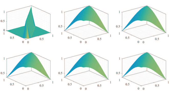
Figure 1: Iterations of simulated covariance functions $\left\{{{T^{\left(k\right)}}}\right\}_{k=0}^{5}$.

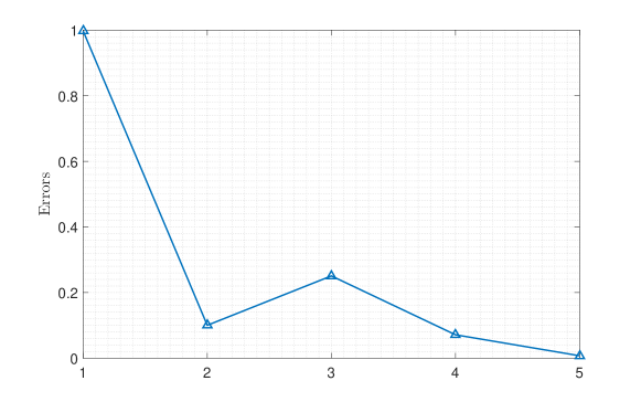
Figure 2: Iterative errors.

In order to verify the performances of the porposed methods, we utilize Algorithm 2, Algorithm 3 and Algorithm 4 to represent obtained stochastic samples, respectively. For Algorithm 3, Fig.3 shows first four eigenfunctions and eigenvalues of $C\left({{x_{1}},{x_{2}}}\right)$ obtained by Eq.(13).

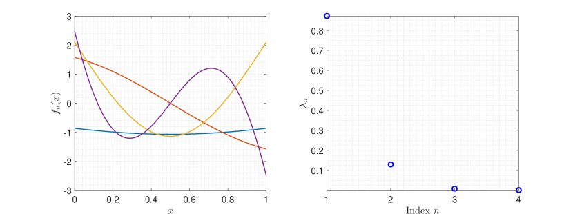
Figure 3: Eigenfunctions (left) and eigenvalues (right) of covariance $C\left({{x_{1}},{x_{2}}}\right)$.

Fig.4 shows cumulative distribution functions (CDFs) of random variables $\left\{{{\xi_{i}}\left(\theta\right)}\right\}_{i=1}^{4}$ computed by Eq.(15) and Table.1 indicates that they are uncorrelated random variables, which is consistent with the theory of KL expansion.

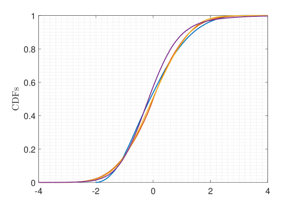
Figure 4: CDFs of random variables $\left\{{{\xi_{i}}\left(\theta\right)}\right\}_{i=1}^{4}$.

Table 1: Statistical correlations between ${\xi_{i}}\left(\theta\right)$ and ${\xi_{j}}\left(\theta\right)$

$E\left\{{{\xi_{i}}{\xi_{j}}}\right\}$	${\xi_{1}}\left(\theta\right)$	${\xi_{2}}\left(\theta\right)$	${\xi_{3}}\left(\theta\right)$	${\xi_{4}}\left(\theta\right)$
${\xi_{1}}\left(\theta\right)$	1.0005
${\xi_{2}}\left(\theta\right)$	0.0004	0.9995		sym.
${\xi_{3}}\left(\theta\right)$	0.0042	0.0016	0.9927
${\xi_{4}}\left(\theta\right)$	0.0272	0.0087	$-$0.0082	1.0248

Fig.5 shows comparisons between target (top left), sample (top mid) and KL-simulated (top right) covariance. The relative errors between target and sample covariance (bottom left), target and KL-simulated covariance (bottom mid) and sample and KL-simulated covariance (bottom right) demonstrate the high accuracy of the proposed Algorithm 2.

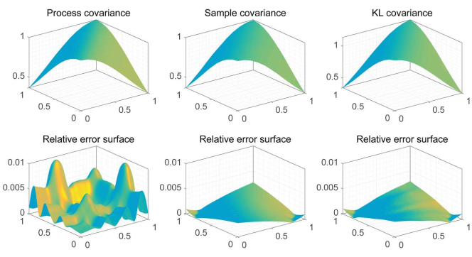
Figure 5: Comparisons between target, sample and KL-simulated covariance.

For Algorithm 3, we adopt 2-order Hermite Polynomial Chaos basis, the number of total terms $M$ is 14. Fig.6 shows $\left\{{{f_{i}}\left(x\right)}\right\}_{i=1}^{P}$ obtained by Eq.(17).

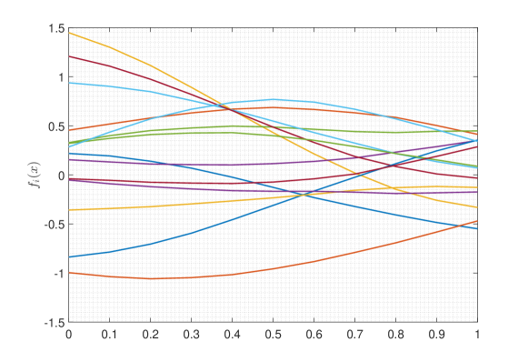
Figure 6: Coefficient functions $\left\{{{f_{i}}\left(x\right)}\right\}_{i=}^{14}$ of PC expansion.

Comparisons between target, sample and PC-simulated covariance (the corresponding legends of relative errors are the same as Fig.5) are shown in Fig.7, which demonstrates the high accuracy of the proposed Algorithm 3.

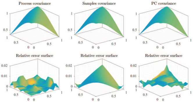
Figure 7: Comparisons between target, sample and PC-simulated covariance.

For Algorithm 4, Table.2 shows projection coefficients $c_{ij}$ obtained by Eq.(20) and comparisons between target, sample and KL-PC-simulated covariance (the corresponding legends of relative errors are the same as Fig.5) are shown as Fig.8, which demonstrates the high accuracy of the proposed Algorithm 4.

Table 2: Coefficients $c_{ij}$ of the KL-PC expansion

$c_{ij}$	1	2	3	4	5	6	7
1	$-$0.2273	$-$0.3286	$-$0.6603	$-$0.4586	0.0511	0.5482	0.3417
2	$-$0.3109	0.8586	0.2774	0.5514	$-$0.9518	$-$0.6500	$-$0.6917
3	0.3333	$-$0.0232	1.1992	$-$0.1781	0.3611	0.0587	$-$0.3919
4	$-$0.3514	$-$1.0478	0.7115	$-$0.1398	1.4399	1.0510	0.5405
$c_{ij}$	8	9	10	11	12	13	14
1	0.2638	$-$0.0346	$-$0.0014	0.3181	$-$0.3325	$-$0.5259	0.7197
2	0.4569	0.0296	0.7990	$-$0.3317	$-$0.2799	$-$0.0816	0.2825
3	$-$1.0618	0.7456	0.3166	$-$0.6234	0.2455	$-$0.1098	$-$0.4125
4	$-$1.3680	$-$0.2531	$-$0.2757	$-$0.3412	0.0206	$-$0.1233	$-$0.9378

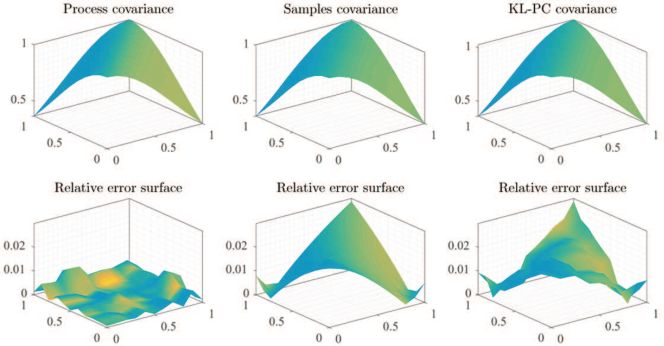
Figure 8: Comparison between target, sample and KL-PC-simulated covariance.

4.2 Example 2: non-gaussian and non-stationary stochastic process

Consider the stochastic process with beat marginal distribution function in Eq.(21) and Brown-Bridge covariance function [21]

$$C\left({{x_{1}},{x_{2}}}\right)=\min\left({{x_{1}},{x_{2}}}\right)-{x_{1}}{x_{2}}$$ (25)

According to Eq.(25), we can obtain $\sigma_{F}^{2}\left(x\right)=C\left({x,x}\right)=x-{x^{2}}$. Letting ${\mu_{F}}\left(x\right)=0$ and solving Eq.(24) yields,

$${y_{\min}}=-\sqrt{14\left({x-{x^{2}}}\right)},~{}{y_{\max}}=\sqrt{3.5\left({x-{x^{2}}}\right)}$$ (26)

Fig.9 shows iterations of sample covariance functions $\left\{{{T^{\left(k\right)}}}\right\}_{k=0}^{4}$ and Fig.10 shows convergence error in each iteration, which once again demonstrate the good convergence and the high accuracy of Algorithm 1.

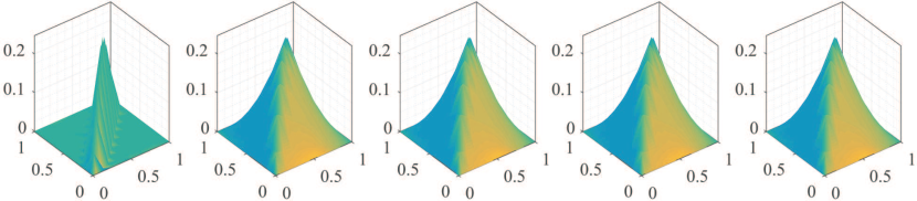
Figure 9: Iterations of sample covariance functions $\left\{{{T^{\left(k\right)}}}\right\}_{k=0}^{4}$.

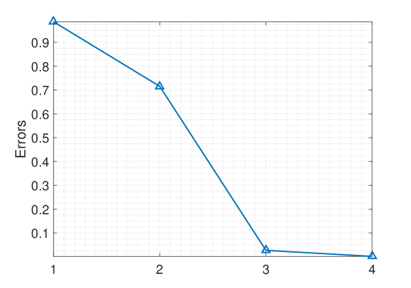
Figure 10: Iterative errors.

Example 4.1 validate Algorithm 2, Algorithm 3 and Algorithm 4, here we only consider using Algorithm 2 expand the obtained stochastic samples from Algorithm 1. According to Eq.(13), analytical eigenfunctions and eigenvalues of $C\left({{x_{1}},{x_{2}}}\right)$ can be obtained as

$${f_{k}}\left(x\right)=\sqrt{2}\sin k\pi x,~{}{\lambda}_{k}=\frac{1}{{{k^{2}}{\pi^{2}}}},~{}k=1,2,\cdots$$ (27)

First six eigenfunctions and eigenvalues are shown in Fig.11.

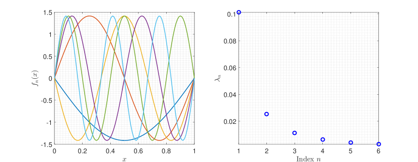
Figure 11: Eigenfunctions (left) and eigenvalues (right) of covariance $C\left({{x_{1}},{x_{2}}}\right)$.

Fig.12 shows CDFs of random variables $\left\{{{\xi_{i}}\left(\theta\right)}\right\}_{i=1}^{6}$ and they are uncorrelated as shown as Table.3, which is once again consistent with the theory of KL expansion. Fig.13 shows comparisons between target, sample and KL-simulated covariance (the corresponding legends of relative errors are the same as Fig.5), which verify the applicability of the proposed Algorithm 2 to non-gaussian and non-stationary stochastic processes.

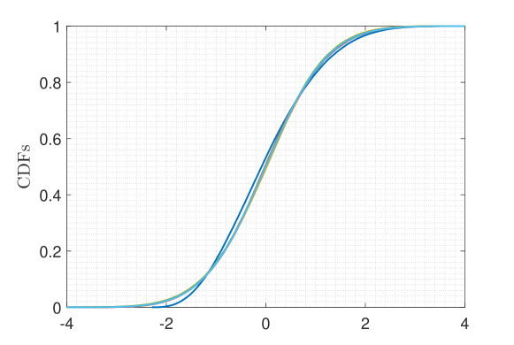
Figure 12: CDFs of random variables $\left\{{{\xi_{i}}\left(\theta\right)}\right\}_{i=1}^{6}$.

Table 3: Statistical correlations between ${\xi_{i}}\left(\theta\right)$ and ${\xi_{j}}\left(\theta\right)$

$E\left\{{{\xi_{i}}{\xi_{j}}}\right\}$	${\xi_{1}}\left(\theta\right)$	${\xi_{2}}\left(\theta\right)$	${\xi_{3}}\left(\theta\right)$	${\xi_{4}}\left(\theta\right)$	${\xi_{5}}\left(\theta\right)$	${\xi_{6}}\left(\theta\right)$
${\xi_{1}}\left(\theta\right)$	0.9991
${\xi_{2}}\left(\theta\right)$	$-$0.0010	1.0006
${\xi_{3}}\left(\theta\right)$	$-$0.0025	0.0015	1.0005		sym.
${\xi_{4}}\left(\theta\right)$	$-$0.0011	0.0017	0.0004	1.0001
${\xi_{5}}\left(\theta\right)$	$-$0.0004	0.0006	$-$0.0010	$-$0.0006	1.0000
${\xi_{6}}\left(\theta\right)$	0.0026	$-$0.0009	$-$0.0003	0.0009	0.0005	0.9999

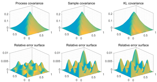
Figure 13: Comparisons between target, sample and KL-simulated covariance.

4.3 Example 3: strongly non-gaussian and non-stationary stochastic process

Consider a stochastic process with shifted lognormal marginal distribution proposed in [21]

$$F\left({y;\mu,\delta,\sigma}\right)=\Phi\left({\frac{{\ln\left({y-\delta\left(x\right)}\right)-\mu\left(x\right)}}{\sigma}}\right)$$ (28)

and covariance function

$$C\left({{x_{1}},{x_{2}}}\right)=e^{-\left({{x_{1}}+{x_{2}}}\right)-\left|{{x_{1}}-{x_{2}}}\right|}$$ (29)

The expectation function and variance function of the shifted lognormal distribution in Eq.(28) are

$$\left\{\begin{array}[]{l}{\mu_{F}}\left(x\right)=\delta\left(x\right)+{e^{\mu\left(x\right)+\frac{1}{2}{\sigma^{2}}}}\\ \sigma_{F}^{2}\left(x\right)=\left({{e^{{\sigma^{2}}}}-1}\right){e^{2\mu\left(x\right)+{\sigma^{2}}}}\end{array}\right.$$ (30)

According to Eq.(29), the variance function is $\sigma_{F}^{2}\left(x\right)=C\left({x,x}\right)=e^{-2x}$. Letting ${\mu_{F}}\left(x\right)=0$, $\sigma=1$ and solving Eq.(30) yield $\mu\left(x\right)=-x-\ln\sqrt{e\left({e-1}\right)}\approx-x-0.7707$ and $\delta\left(x\right)=-\frac{{{e^{-x}}}}{{\sqrt{e-1}}}\approx-0.7629{e^{-x}}$.

Fig.14 shows iterations of sample covariance functions $\left\{{{T^{\left(k\right)}}}\right\}_{k=0}^{6}$ and the corresponding convergence error of each iteration is shown as Fig.15. The good convergence of Algorithm 2 for non-gaussian and non-stationary stochastic processes is demonstrated.

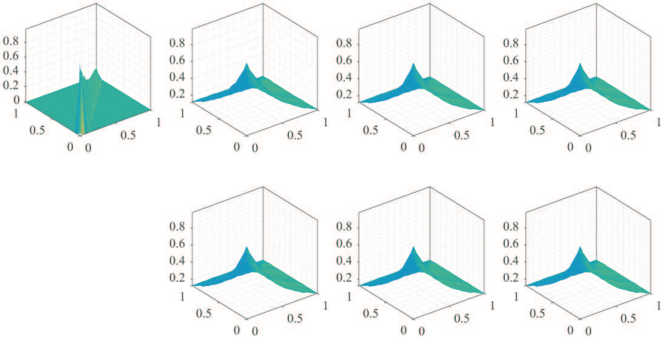
Figure 14: Iterations of sample covariance functions $\left\{{{T^{\left(k\right)}}}\right\}_{k=0}^{6}$.

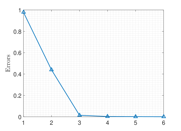
Figure 15: Iterative errors.

According to Eq.(13), first six eigenfunctions and eigenvalues of $C\left({{x_{1}},{x_{2}}}\right)$ are shown in Fig.16.

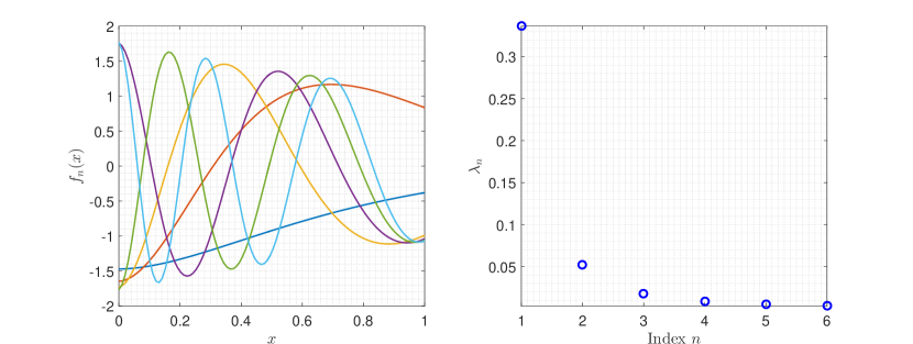
Figure 16: Eigenfunctions (left) and eigenvalues (right) of covariance $C\left({{x_{1}},{x_{2}}}\right)$.

Fig.17 shows CDFs of random variables $\left\{{{\xi_{i}}\left(\theta\right)}\right\}_{i=1}^{6}$ and their uncorrelated properties are shown as Table.4. Fig.18 shows comparisons between target, sample and KL-simulated covariance (the corresponding legends of relative errors are the same as Fig.5), which verify the applicability of the proposed Algorithm 2 to strongly non-gaussian and non-stationary stochastic processes.

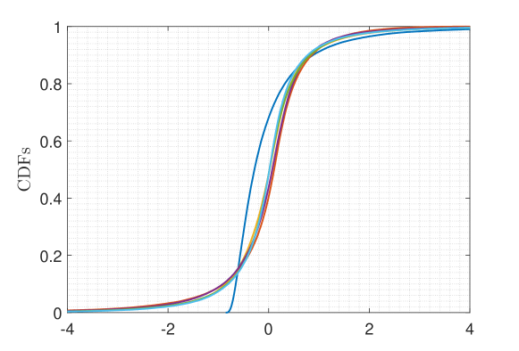
Figure 17: CDFs of random variables $\left\{{{\xi_{i}}\left(\theta\right)}\right\}_{i=1}^{6}$.

Table 4: Statistical correlations between ${\xi_{i}}\left(\theta\right)$ and ${\xi_{j}}\left(\theta\right)$

$E\left\{{{\xi_{i}}{\xi_{j}}}\right\}$	${\xi_{1}}\left(\theta\right)$	${\xi_{2}}\left(\theta\right)$	${\xi_{3}}\left(\theta\right)$	${\xi_{4}}\left(\theta\right)$	${\xi_{5}}\left(\theta\right)$	${\xi_{6}}\left(\theta\right)$
${\xi_{1}}\left(\theta\right)$	1.0051
${\xi_{2}}\left(\theta\right)$	$-$0.0015	0.9979
${\xi_{3}}\left(\theta\right)$	$-$0.0148	0.0014	1.0049		sym.
${\xi_{4}}\left(\theta\right)$	0.0141	0.0004	$-$0.0028	0.9988
${\xi_{5}}\left(\theta\right)$	$-$0.0050	0.0066	0.0077	0.0038	0.9997
${\xi_{6}}\left(\theta\right)$	$-$0.0093	0.0069	0.0029	$-$0.0076	0.0061	1.0042

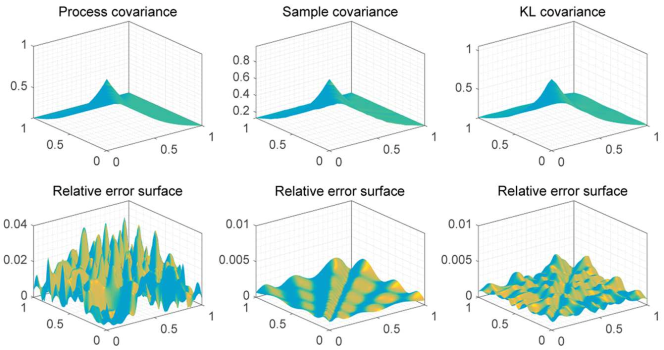
Figure 18: Comparisons between target, sample and KL-simulated covariance.

5 Conclusion

In this paper, efficient numerical schemes have been presented for simulating non-gaussian and non-stationary stochastic processes specified by covariance functions and marginal distribution functions. In order to simulate samples of the target stochastic process, stochastic samples automatically matching the target marginal distribution function are firstly generated, and an iterative algorithm is proposed to match the target covariance function by transform the order of initial stochastic samples. Three numerical examples demonstrate the fast convergence and the high accuracy of the proposed algorithm. In order to overcome the difficulty that sample-descriptions are not convenient to applied to subsequent stochastic analysis, three numerical algorithms are developed to represent the obtained stochastic samples based on KL expansion and PC expansion. Different algorithms can be used for different problems of practical interests and the performances of the developed algorithms are indicated by numerical examples. All proposed algorithms can be readily extended to multi-dimensional random fields and will be shown in subsequent researches.

References

- Ghanem and Spanos [2003] R. G. Ghanem, P. D. Spanos, Stochastic finite elements: a spectral approach, Courier Corporation, 2003.
- Tankov [2003] P. Tankov, Financial modelling with jump processes, Chapman and Hall/CRC, 2003.
- Aboy et al. [2005] M. Aboy, O. W. Márquez, J. McNames, R. Hornero, T. Trong, B. Goldstein, Adaptive modeling and spectral estimation of nonstationary biomedical signals based on kalman filtering, IEEE Transactions on Biomedical Engineering 52 (2005) 1485–1489.
- Stefanou [2009] G. Stefanou, The stochastic finite element method: past, present and future, Computer methods in applied mechanics and engineering 198 (2009) 1031–1051.
- Papoulis and Pillai [2002] A. Papoulis, S. U. Pillai, Probability, random variables, and stochastic processes, Tata McGraw-Hill Education, 2002.
- Grigoriu [2006] M. Grigoriu, Evaluation of karhunen–loève, spectral, and sampling representations for stochastic processes, Journal of engineering mechanics 132 (2006) 179–189.
- Rasmussen [2003] C. E. Rasmussen, Gaussian processes in machine learning, in: Summer School on Machine Learning, Springer, 2003, pp. 63–71.
- Phoon et al. [2004] K. Phoon, H. Huang, S. Quek, Comparison between karhunen–loeve and wavelet expansions for simulation of gaussian processes, Computers & structures 82 (2004) 985–991.
- Deodatis and Micaletti [2001] G. Deodatis, R. C. Micaletti, Simulation of highly skewed non-gaussian stochastic processes, Journal of engineering mechanics 127 (2001) 1284–1295.
- Yamazaki and Shinozuka [1988] F. Yamazaki, M. Shinozuka, Digital generation of non-Gaussian stochastic fields, Journal of Engineering Mechanics 114 (1988) 1183–1197.
- Shinozuka and Deodatis [1991] M. Shinozuka, G. Deodatis, Simulation of stochastic processes by spectral representation, Applied Mechanics Reviews 44 (1991) 191–204.
- Elishakoff et al. [1994] I. Elishakoff, Y. J. Ren, M. Shinozuka, Conditional simulation of non-gaussian random fields, Engineering Structures 16 (1994) 558–563.
- Popescu et al. [1998] R. Popescu, G. Deodatis, J. H. Prevost, Simulation of homogeneous nongaussian stochastic vector fields, Probabilistic Engineering Mechanics 13 (1998) 1–13.
- Grigoriu [1998] M. Grigoriu, Simulation of stationary non-Gaussian translation processes, Journal of engineering mechanics 124 (1998) 121–126.
- Liu et al. [2016] Z. Liu, W. Liu, Y. Peng, Random function based spectral representation of stationary and non-stationary stochastic processes, Probabilistic Engineering Mechanics 45 (2016) 115–126.
- Huang et al. [2001] S. Huang, S. Quek, K. Phoon, Convergence study of the truncated karhunen–loeve expansion for simulation of stochastic processes, International journal for numerical methods in engineering 52 (2001) 1029–1043.
- Sudret and Der Kiureghian [2000] B. Sudret, A. Der Kiureghian, Stochastic finite elements and reliability: a state-of-the-art report, University of California, Berkeley (2000) 114–120.
- Poirion and Zentner [2013] F. Poirion, I. Zentner, Non-gaussian non-stationary models for natural hazard modeling, Applied Mathematical Modelling 37 (2013) 5938–5950.
- Kim and Shields [2015] H. Kim, M. D. Shields, Modeling strongly non-gaussian non-stationary stochastic processes using the Iterative Translation Approximation Method and Karhunen–Loève expansion, Computers & Structures 161 (2015) 31–42.
- Liu et al. [2017] Z. Liu, Z. Liu, Y. Peng, Dimension reduction of Karhunen-Loeve expansion for simulation of stochastic processes, Journal of Sound and Vibration 408 (2017) 168–189.
- Phoon et al. [2002] K. Phoon, S. Huang, S. Quek, Simulation of second-order processes using Karhunen–Loeve expansion, Computers & structures 80 (2002) 1049–1060.
- Phoon et al. [2005] K. Phoon, H. Huang, S. Quek, Simulation of strongly non-Gaussian processes using Karhunen–Loeve expansion, Probabilistic Engineering Mechanics 20 (2005) 188–198.
- Dai et al. [2019] H. Dai, Z. Zheng, H. Ma, An explicit method for simulating non-gaussian and non-stationary stochastic processes by Karhunen–Loève and polynomial chaos expansion, Mechanical Systems and Signal Processing 115 (2019) 1–13.
- Sakamoto and Ghanem [2002a] S. Sakamoto, R. Ghanem, Polynomial chaos decomposition for the simulation of non-Gaussian nonstationary stochastic processes, Journal of engineering mechanics 128 (2002a) 190–201.
- Sakamoto and Ghanem [2002b] S. Sakamoto, R. Ghanem, Simulation of multi-dimensional non-gaussian non-stationary random fields, Probabilistic Engineering Mechanics 17 (2002b) 167–176.
- Puig et al. [2002] B. Puig, F. Poirion, C. Soize, Non-Gaussian simulation using hermite polynomial expansion: convergences and algorithms, Probabilistic Engineering Mechanics 17 (2002) 253–264.
- Field Jr and Grigoriu [2004] R. Field Jr, M. Grigoriu, On the accuracy of the polynomial chaos approximation, Probabilistic Engineering Mechanics 19 (2004) 65–80.
- Lagaros et al. [2005] N. D. Lagaros, G. Stefanou, M. Papadrakakis, An enhanced hybrid method for the simulation of highly skewed non-gaussian stochastic fields, Computer Methods in Applied Mechanics and Engineering 194 (2005) 4824–4844.
- Zheng and Dai [2017] Z. Zheng, H. Dai, Simulation of multi-dimensional random fields by Karhunen–Loève expansion, Computer Methods in Applied Mechanics and Engineering 324 (2017) 221–247.
- Betz et al. [2014] W. Betz, I. Papaioannou, D. Straub, Numerical methods for the discretization of random fields by means of the Karhunen–Loève expansion, Computer Methods in Applied Mechanics and Engineering 271 (2014) 109–129.
- Christou et al. [2016] V. Christou, P. Bocchini, M. J. Miranda, Optimal representation of multi-dimensional random fields with a moderate number of samples: Application to stochastic mechanics, Probabilistic Engineering Mechanics 44 (2016) 53–65.
- Xiu [2010] D. Xiu, Numerical methods for stochastic computations: a spectral method approach, Princeton university press, 2010.