The Decision-Conflict Logit

Abstract

We introduce the decision-conflict logit, a simple and disciplined extension of the logit with an outside option that assigns a menu-dependent utility to that option. The relative value of this utility at a menu could be interpreted as proxying decision difficulty and determines the probability of avoiding/delaying choice at that menu. We focus on two intuitively structured special cases of the model that offer complementary insights, and argue that they explain a variety of observed choice-deferral effects that are caused by hard decisions. We conclude by illustrating the usability of the proposed modelling framework in applications.

Keywords: decision difficulty; quadratic logit; reciprocal utility differences; discrete choice; price-quality competition; choice deferral; choice architecture.

1     Introduction

It is a well-established fact that people often opt for the choice-deferral outside option when they find it hard to compare the active-choice alternatives available to them, even when these alternatives are individually considered “good enough” to be chosen and are paid attention to. Realistic examples of such behaviour include: (i) employees who operated within an “active decision” pension-savings environment and did not sign up for one of the plans that were available to them within, say, a day, week or month of first notice, possibly even opting for indefinite non-enrolment; (ii) patients who, instead of choosing “immediately” one of the active treatments that were recommended to them against a medical condition, delayed making such a choice -often at a health cost- due to “facing a treatment dilemma”; (iii) doctors who were willing to prescribe the single available drug to treat a medical condition but were not prepared to prescribe anything when they had to decide from the expanded set that contained one more drug, because “the difficulty in deciding between the two medications led some physicians to recommend not starting either” (Redelmeier and Shafir, 1995).

Motivated by the relevance of opting-out decisions for understanding preferences and explaining behaviour, our goal in this paper is to model choice in the presence of a choice-deferral outside option within a stochastic choice framework in ways that deviate as little as possible from existing well-understood modelling practices and, at the same time, reflect some important findings in the relevant empirical/experimental literature. We pursue this by extending in disciplined ways the foundational Luce (1959)/logit model. Specifically, we propose and study the class of decision-conflict logit models which, in their most general form, are a straightforward but so far unexplored extension of the logit with an outside option that assign a menu-dependent utility to that option while retaining the menu-invariance assumption on all active-choice alternatives. The relative value of outside-option utility at a menu in turn determines the probability of avoiding/deferring choice and can be interpreted as proxying decision difficulty. Despite its simplicity, this baseline general model can be used to analyse numerous richly structured special cases. We introduce and focus on two such cases where decision difficulty depends in intuitive ways on the utilities of all active-choice alternatives.

In the first such special case, decision difficulty could be thought of as driven by the agent’s noisy resampling of the menu’s elements. More specifically, in our quadratic logit model such resampling takes the form of the choice probability of a market alternative emerging as the product of two logit probabilities according to a single value function/criterion. Intuitively, the agent is more likely to choose an active-choice alternative iff its value realizations according to this criterion are much larger than those of everything else feasible across both rounds of sampling. Conversely, the agent is more likely to avoid/defer choice when no alternative achieves such unanimous clear dominance. This model could therefore be thought of as capturing a hesitant decision maker who behaves as if they used an objective criterion to compare alternatives (e.g. sum or multiply each option’s values across all relevant attributes) but is aware that their subjective evaluation according to this objective criterion may be imperfect, possibly due to cognitive limitations, thereby leading them to performing this task twice.

Our second special case on the other hand has the property that decision difficulty at each binary menu is decreasing in the utility difference between the two alternatives of that menu. We focus on the reciprocal utility differences specification which, although in many ways different, is inspired by the influential drift-diffusion neuroeconomic model that is considered very successful in psychology and neuroscience, and which has also been of increasing interest to economists recently (Milosavljevic et al., 2010; Krajbich et al., 2010; Alós-Ferrer et al., 2021). At the heart of the axiomatic structure of all models in this paper is the so far unexplored version of the Luce/Independence of Irrelevant Alternatives axiom where its odds-invariance restrictions are required to apply over pairs of active-choice alternatives but not on pairs that involve such an alternative and the outside option. The two special cases, moreover, are characterized by means of novel and interpretable additional axioms that impose intuitive restrictions on the odds of deferring/not deferring at binary menus and/or their interplay with the relative choice probabilities of market alternatives at those menus.

We show that the quadratic logit and reciprocal-differences models explain the following empirical phenomena that many studies in cognitive and consumer psychology have documented about non-forced choice decisions:

1. the dominance-driven non-monotonic relation between menu expansion and the tendency to opt out –we refer to it as the “roller-coaster” choice-overload effect– which has implications for the interpretation and policy responses to choice overload phenomena;

2. “absolute attractiveness” effects, whereby increasing the total utility of all alternatives in a menu while holding their utility differences constant increases the probability of an active choice;

3. “relative attractiveness” effects, whereby holding the total utility of all alternatives in a menu constant while increasing their utility differences increases the probability of an active choice;

4. similarity-driven deferral effects, whereby lower utility differences between two alternatives increase the probability of choice delay.

We illustrate the economic applicability of our general modelling and its two structured special cases. Motivated by and applying in our framework the findings from recent experimental evidence and theoretical models of simplicity-seeking in choice under risk, we first explore how a preference-for-simplicity specification of the baseline decision-conflict logit predicts when the decision maker is more likely to choose a simple lottery and when they are more likely to delay choice if they are assumed to operate in a non-forced-choice environment. We also discuss the implications of this analysis for optimal choice architecture. Next, we show how the classic assumptions and argument that underpin the conditional-logit formulation of the logit without an outside option (McFadden, 1973) can be modified/extended in simple ways in order for the quadratic logit to admit a similar conditional/discrete-choice formulation. Third, we analyse a duopolistic model where firms simultaneously compete in price and quality under logit and quadratic-logit demand. We find that the quadratic-logit equilibrium has both firms increasing their products’ quality/price ratio by 50% relative to the baseline logit equilibrium, and seeing their profits decreased by almost two thirds. Intuitively, each firm increases its quality/price ratio in an effort to reduce the consumer’s decision difficulty and mitigate the risk of losing them to the rival firm or driving them out of the market altogether.

The remaining parts of the paper are organized as follows. Section 2 introduces the notation and baseline models. Sections 3 and 4 introduce and analyse the quadratic-logit and reciprocal-differences special cases of the general decision-conflict logit model. Sections 5 and 6, respectively, illustrate the two models’ descriptive relevance and applicability. Section 7 relates our work to the existing literature and Section 8 concludes. Unless otherwise noted, all proofs appear in the Appendix. The Online Supplementary Appendix provides characterizations of the class of decision-conflict logit models where the complexity function is monotonic with respect to set inclusion and admits a general utility-difference formulation, respectively.

2     Preliminaries

2.1     A Generalized Luce Model with a Context-Dependent Outside Option

Let $X$ be the grand choice set of finitely many and at least two active-choice alternatives, with generic elements $a,b\in X$. Let $\mathcal{M}:=\{A:\emptyset\neq A\subseteq X\}$ be the collection of all menus of such alternatives, and let $\mathcal{B}$ be its sub-collection that comprises all binary menus of distinct alternatives in $X$. The outside option is denoted by $o\not\in X$. A random non-forced choice model on $X$ is a function $\rho:\mathcal{M}\times\mathcal{M}\rightarrow\mathbb{R}_{+}$ such that $\rho(\{a\},A)\in[0,1]$ for all $A\in\mathcal{M}$ and all $a\in A$; $\rho(\{a\},A)=0$ for all $A\in{\mathcal{M}}$ and all $a\not\in A$; and $\sum_{a\in A}\rho(\{a\},A)\leq 1$, where $\rho(o,A):=1-\sum_{a\in A}\rho(\{a\},A)\leq 1$ is the probability of choosing the –always feasible– outside option at menu $A$. To simplify notation we write $\rho(a,A)\equiv\rho(\{a\},A)$ and, for $A,B\in{\mathcal{M}}$ with $B\subseteq A$, we also let $\rho(B,A):=\sum_{b\in B}\rho(b,A)$. Finally, we will refer to any $\rho$ with the property that $\rho(a,A)\neq\rho(b,A)$ for every menu $A$ and all alternatives $a,b$ in $A$ as asymmetric.

We introduce the generalized Luce model with a context-dependent outside option as the one that comprises a utility function $u:X\rightarrow\mathbb{R}_{++}$ and a function $M:\mathcal{M}\rightarrow\mathbb{R}_{+}$ such that, for every menu $A$ and alternative $a\in A$,

$$\rho(a,A) = \displaystyle\frac{u(a)}{\displaystyle\sum_{b\in A}u(b)+M(A)},$$ (1)

where $(u,M)$ is unique up to a common positive linear transformation. Thus, in this model all active-choice alternatives are assigned menu-independent Luce utility values that determine their relative likelihood of being chosen while the probability of making an active choice in the first place (equivalently, of avoiding/deferring this decision) is determined by the menu-dependent Luce utility of the outside option.

The following axioms characterize the class of models that can be represented in this way:

A1 (Positivity).
For all $A\in{\mathcal{M}}$ and all $a\in A$: $\rho(a,A)>0$.

A2 (The Active-Choice Luce Axiom).
For all $A,B\in{\mathcal{M}}$ and all $a,b\in A\cap B$:

$$\frac{\rho(a,A)}{\rho(b,A)} = \frac{\rho(a,B)}{\rho(b,B)}$$

A1 is standard and allows for a crisper illustration of the main ideas that we put forward in this paper. A2 imposes the standard kind of IIA-consistency only in the odds of pairs of active-choice alternatives while allowing odds that involve such an alternative and the outside option to deviate from it. That is, $\frac{\rho(o,A)}{\rho(b,A)}\neq\frac{\rho(o,B)}{\rho(b,B)}$ is possible. Gerasimou (2018); Costa-Gomes, Cueva, Gerasimou, and Tejiščák (2022) have recently argued on theoretical and empirical grounds that deterministic revealed preferences may be more likely to conform to no-cycle principles of consistency when active choices are not forced upon decision makers than when they are forced. Therefore, a reasonable testable hypothesis is that the descriptive appeal of A2 as an approximation of observed behaviour may be increased in the non-forced random choice environment considered in this paper compared to the Luce/IIA axiom under the standard forced-choice setting.

Proposition 1

A random non-forced choice model $\rho$ is a generalized Luce model with a context-dependent outside option iff it satisfies A1-A2.

Indeed, by adapting the arguments in Luce (1959) one obtains an equivalence between A1-A2 and the existence of a function $u:X\rightarrow\mathbb{R}_{++}$ such that, for every $A\in{\mathcal{M}}$ and $a\in A$,

$$\rho(a,A) = \big{(}1-\rho(o,A)\bigr{)}\cdot\frac{u(a)}{\displaystyle\sum_{b\in A}u(b)},$$ (2)

where

$$u(a) := \alpha\cdot\frac{\rho(a,X)}{\rho(z,X)}$$ (3)

for arbitrary and fixed $\alpha>0$ and $z\in X$. It follows then that for every $A\in{\mathcal{M}}$ there is a unique $M(A)\geq 0$ that makes (1) true, with

$$M(A) \equiv \frac{\rho(o,A)}{1-\rho(o,A)}\cdot\sum_{b\in A}u(b).$$ (4)

Finally, it is immediate that $(u,M)$ and $(u^{\prime},M^{\prime})$ represent the same $\rho$ if and only if $u=\alpha u^{\prime}$ and $M=\alpha M^{\prime}$ for some $\alpha>0$.

We now compare (1) to the baseline Luce (1959) model (henceforth logit) with an outside option (Anderson et al., 1992; Hensher et al., 2015), and to the one without such an option. To this end, recall that a random non-forced choice model $\rho$ on $X\cup\{o\}$ admits the former representation if there is a function $u:X\cup\{o\}\rightarrow\mathbb{R}_{++}$ such that, for all $A\in{\mathcal{M}}$ and $a\in A$,

$$\rho(a,A) = \frac{u(a)}{\displaystyle\sum_{b\in A}u(b)+u(o)},$$ (5)

where $u(o)>0$ is menu-independent. On the other hand, $\rho$ admits a logit representation without an outside option if there exists some $u:X\rightarrow\mathbb{R}_{++}$ such that, for all $A\in{\mathcal{M}}$ and $a\in A$,

$$\rho(a,A) = \frac{u(a)}{\displaystyle\sum_{b\in A}u(b)},$$ (6)

which obviously implies $\sum_{a\in A}\rho(a,A)=1$ for all $A\in{\mathcal{M}}$, so that the opportunity to defer is either infeasible or feasible but never acted upon. Thus, (1) includes (6) as a special case when $o\not\in X$, and (1) modifies (5) without nesting it unless A1-A2 operate on the enriched domain $X\cup\{o\}$.

We note, finally, that despite the simplicity of (1) and the complete straightforwardness of Proposition 1, the hereby proposed extension of the baseline logit models is to our knowledge new. As we show in the sequel, moreover, several interesting and non-trivial new insights are derived from this simple specification once intuitive structures are imposed on $u$ and/or $D$. Furthermore, as (4) clarifies, and as will be clarified further later on, any additional structure that is imposed on $u$ and/or $D$ translates into restrictions on the interplay between the odds of opting out relative to making an active choice at a menu on the one hand, and the normalized choice probabilities of the various feasible alternatives on the other. In what follows we will be introducing interpretable axioms from this novel class and study their powerful interactions with A2 for a particular family of random non-forced choice models that satisfy (1). In light of these remarks, therefore, it should be clear that the main purpose of introducing (1) and describing its axiomatic structure in this section is to clarify the general behavioural origins of the more novel and richly structured models that follow and elucidate how (dis)similar these are to the familiar models captured in (5) and (6).

2.2     The Baseline Decision-Conflict Logit

As was mentioned in the Introduction, this paper’s goal is to contribute towards the modelling of decision difficulty that is rooted in a fully attentive individual’s potential inability to make some preference comparisons between otherwise desirable options. If a single such option was feasible to such an individual, therefore, one might expect that person to immediately choose that one option. If on the other hand there are at least two available options and the individual is not forced to make a choice immediately, then the experimental/empirical evidence suggests that there is at least some probability that this person’s attempt to find a most preferred option and choose that option will not be fruitful reasonably quickly. To the extent that this is so, a legitimate approach from the analyst’s perspective would be to portray that decision maker as deferring choice with positive probability whenever at least one non-trivial comparison is required.

Imagine, for example, a patient as in Knops et al. (2013) who has been diagnosed with a life-threatening disease. Suppose that their doctor informs them that there is only one available treatment that can cure this disease, and asks whether they would like to sign up for this treatment. One would expect the patient to sign up immediately because there would be no benefit from delaying their only chance for a cure. Now suppose instead that the doctor tells the patient that there are two possible treatments: one with high efficacy but severe side effects, and another with milder side effects but lower cure rates. Although if either of these was the only feasible treatment it would have been chosen immediately, in this case one might expect the patient to delay making such an active choice, perhaps until they think about the conflicting pros and cons and then ultimately determine which treatment would be best for them. Situations of this kind are compatible with and, in fact, motivate the modelling framework and axioms in this study.

We model these ideas with the following axiom:

A3 (Desirability & Complexity)
For all $A\in{\mathcal{M}}$: $\rho(A,A)=1$ $\Longleftrightarrow$ $|A|=1$.

In words, A3 postulates that an active choice is made with certainty only at singleton menus and, as such, it formalises the behavioural mechanisms outlined above. Of course, one can still think of situations where this axiom is descriptively invalid. Yet, for analytical purposes it is a useful property because it allows for completely isolating the decision-difficulty channel to deferrals from other potential channels such as undesirability of the available alternatives or limited attention, which have quite distinct behavioural origins.

In light of the analysis in the preceding subsection, the next result is immediate:

Corollary 1

A random non-forced choice model $\rho$ satisfies A1–A3 iff it is representable as in (1) for some pair $(u,M)$ with the property that

$$M(A)=0 \Longleftrightarrow |A|=1.$$ (7)

We will refer to this special class of generalized logit models with a context-dependent outside option as the class of decision-conflict logit models, and to the menu function $M$ that captures the varying appeal of opting out at different menus as the decision cost or decision complexity function, and denote it by $D$.

Justifying such a name for the function $D$ given the requirement that it be zero-valued only at singletons may benefit from some explanation that would supplement the preceding discussion. When the decision environment is such that avoidance/deferral is caused solely by decision difficulty instead of other factors (e.g. none of the active-choice alternatives is good enough, or none is considered due to limited-attention constraints), our decision maker is portrayed as not having any problem deciding between deferring or choosing the only available active-choice option: they do the latter. By contrast, the decision between deferring or choosing from two or more such options is at least somewhat costly because of the effort that is necessary to make the relevant preference comparisons.

Before endogenizing $D$ in the models studied in the next two sections we will focus on an intuitive structural property of this function, and also point out some interesting behavioural implications. In particular, we will refer to both a decision-conflict logit $\rho=(u,D)$ and $D$ as monotonic if

$$A\supset B \Longrightarrow D(A)\geq D(B).$$ (8)

If $D(A)>D(B)$ is always true when $A\supset B$, then $D$ and $\rho=(u,D)$ will be called strictly monotonic. In line with our intended interpretation of $D$ as a complexity/cost function, the total number of pairs of distinct alternatives increases as a menu expands, and therefore so does the expected number of comparisons between alternatives that a fully-attentive individual needs to make. In expectation, therefore, decision difficulty also goes up in absolute terms when more alternatives are added to a menu. Importantly, however, this does not imply that deferring always becomes more likely once a menu is expanded when $D$ is monotonic. We will return to this important point in Section 5.

Monotonicity, however, does have a familiar general implication for active-choice alternatives that, in forced-choice random-utility environments, was originally stated in Block and Marschak (1960):

Observation 1 (Active-Choice Regularity)

If $\rho$ is a monotonic decision-conflict logit, then $a\in B\subset A$ implies $\rho(a,B)>\rho(a,A)$.

This property therefore rules out well-known context-dependent choice phenomena such as the attraction and compromise effects.

3     First Special Case: Quadratic Logit

We now introduce and focus on the random non-forced choice model $\rho$ on $X$ that is defined by the existence of a single function $\widehat{u}:X\rightarrow\mathbb{R}_{++}$ such that, for every menu $A$ and alternative $a$ in $A$,

$$\rho(a,A) = \left(\frac{\widehat{u}(a)}{\sum\limits_{b\in A}\widehat{u}(b)}\right)^{2}.$$ (9)

The agent portrayed in (9) could be thought of as behaving according to the standard logit rule with a single value criterion but, possibly aware of their decision difficulty, also as if they sampled all alternatives twice according to that criterion before making a decision. In this case, because the resulting value realizations generally differ across the two rounds of sampling due to the postulated randomness, the agent can be thought of as being more likely to choose an active-choice alternative if its perceived signal/stimulus intensity from both inspections, captured by the two value realizations of $\widehat{u}$, is relatively high, and as being more likely to avoid/defer choice when this is not true for any such alternative.

When deciding which insurance plan to buy, for example, one may review the top-rated plans from a service comparison website in the morning, receive some value stimuli/signals from each of them, and then go back and repeat this process in the evening. Assuming that the two sampling rounds are independent (admittedly, a demanding assumption), an insurance plan is more likely to be chosen at the end of this two-stage process if its relative stimulus/signal intensity is sufficiently high to make the product stand out despite the agent’s hesitation.

The fact that (9) is a special case of (1) can be verified by letting

$$u(a) := \widehat{u}(a)^{2},$$ (10)

$$D(A) := \left(\sum_{b\in A}\widehat{u}(b)\right)^{2}-\sum_{b\in A}\widehat{u}(b)^{2}$$ (11)

$$= 2\sum_{\begin{subarray}{c}a,b\in A,\\ a\neq b\end{subarray}}\widehat{u}(a)\widehat{u}(b)$$

$$= \sum_{a,b\in A}D(\{a,b\}),$$

where the last step makes use of the notational convention

$$D(\{a,a\}) \equiv D(\{a\}).$$

This also clarifies that the quadratic logit $\rho\equiv(\widehat{u})^{2}$ is an additive decision-conflict logit $(u,D)$ in the sense that the utility of the outside option at every menu depends additively on the utility of that option at each of its binary submenus, and also that the latter takes a symmetric Cobb-Douglas form with respect to $\widehat{u}$. We will return to additivity later in this section.

The next condition on choice probability distributions with a feasible outside option is new, testable and easily seen to be implied by every quadratic logit model.

A4 (Symmetric Deferral Odds)
For all $a,b\in X$:

$$\frac{1}{2}\cdot\frac{\rho(o,\{a,b\})}{\rho(a,\{a,b\})}=\left(\frac{1}{2}\cdot\frac{\rho(o,\{a,b\})}{\rho(b,\{a,b\})}\right)^{-1}$$

A4 requires that the odds of deferring relative to choosing $a$ at menu $\{a,b\}$ be inversely proportional to the odds of deferring relative to choosing $b$ at that menu, with the specific shape of this symmetric non-linear relationship determined by the scalar $\frac{1}{2}$ and depicted in the curve in the simplex of Figure 1. As shown in that figure, in particular, under this axiom the probability of opting out attains its maximum value of 0.5 as $a$ and $b$ become equi-probable. This implication is our first formalization of the idea that decision difficulty is increased when the feasible market alternatives are more or less equally appealing. This discussion suggests that A4 is a potentially good approximation of an individual’s behaviour in cases where: (i) $a$ and $b$ are similarly attractive and this similarity translates into high decision conflict; (ii) $a$ or $b$ is the clearly superior option and choosing it is the most likely decision outcome.

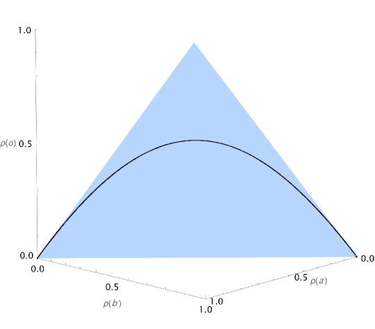
Figure 1: Non-forced binary probability distributions that are compatible with Symmetric Deferral Odds.

The next result provides a partial characterization of the quadratic logit in the class of binary menus $\mathcal{B}$ by means of A4. The general characterization is given later in this section.

Proposition 2

A random non-forced choice model $\rho$ on $X$ is a quadratic logit on the binary menus of $X$ iff it satisfies A1–A4.

Interestingly, the quadratic-logit model’s predicted probability of deferring at a menu as a function of the number of active-choice alternatives at that menu is bounded above in the following simple way:

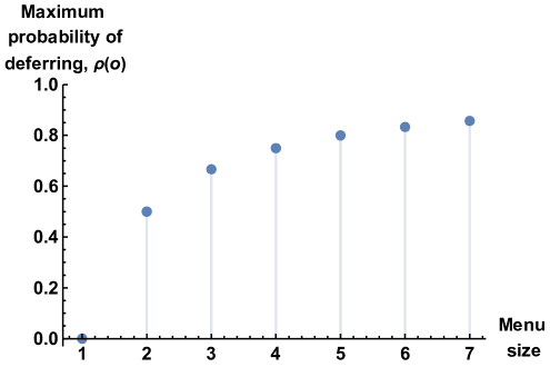
Figure 2: Deferral upper bounds in the quadratic logit as a function of menu size.

Observation 2 (Deferral Upper Bounds in the Quadratic Logit)

If $\rho=(\widehat{u})^{2}$, then, for every menu $A$,

$$\begin{array}[]{lllllll}\rho(o,A)&\leq&1-\dfrac{1}{|A|},&&&\\ \rho(o,A)&=&1-\dfrac{1}{|A|}&\Longleftrightarrow&\widehat{u}(a)=\widehat{u}(b)&\text{for all }a,b\in A.\end{array}$$

In this model, therefore, an agent’s decision difficulty at a menu, as revealed by the deferral probability at that menu, is maximized when all feasible active-choice alternatives are equally desirable, and this maximum difficulty is increasing in proportion to the total number of such alternatives at a decreasing rate (Figure 2).

Turning to the model’s comparative statics in the important class of binary menus, Figure 3 illustrates by example the general pattern in the behaviour of $\rho(a,\{a,b\})$ and $\rho(o,\{a,b\})$ as the stimulus intensity of $a$ changes while that of $b$ is held fixed. Interestingly, the monotonic increase of $\rho(a,\{a,b\})$ in $\widehat{u}(a)$ occurs at an increasing rate as this value approaches the $\frac{\widehat{u}(b)}{2}$ stimulus-intensity threshold from below than when $\widehat{u}(a)$ increases monotonically beyond $\frac{\widehat{u}(b)}{2}$. Intuitively, the inflection-point stimulus intensity value $\frac{\widehat{u}(b)}{2}$ that dissects $\rho(a,\{a,b\})$ –viewed as a function of $\widehat{u}(a)$– into convex and concave regions suggests that marginal improvements in the appeal of $a$ lead to more rapid market share increases when this alternative is still “catching up” with $b$ than when it has become sufficiently close to (or surpassed) it in attractiveness. On the other hand, $\rho(o,\{a,b\})$ is a strictly concave function of $\widehat{u}(a)$ and, consistent with Observation 2, attains its maximum value of $\frac{1}{2}$ when $\widehat{u}(a)=\widehat{u}(b)$.

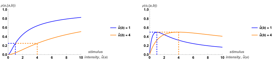
Figure 3: Comparative statics in the quadratic logit when one of the two alternatives becomes more attractive.

Recall now that, as noted in (10), the quadratic logit predicts that decision complexity at any menu with more than two alternatives is additive in the complexity at each of its binary submenus, i.e.

$$D(A) = \sum_{\begin{subarray}{c}a,b\in A\end{subarray}}D(\{a,b\}).$$ (12)

Intuitively, for a decision maker like the one we are modelling in this paper who is paying full attention to all feasible options, all binary comparisons may turn out to be relevant in the search towards determining the overall best alternative in a menu. This is especially so if such a search is inefficient, which is not unlikely for human decision makers. In this case, therefore, the degree of difficulty in identifying such an alternative depends on how hard it is to make every such comparison. Additivity disciplines this monotonic relation in an analytically convenient way.

A5 (Balancing Odds).
For all $A,B\in\mathcal{M}$ with $B\supset A$, and for all $a,b\in A$:

$$\frac{\rho(o,A)}{1-\rho(o,A)}=\sum\limits_{\begin{subarray}{c}a,b\in A,\\ a\neq b\end{subarray}}\left(\frac{\rho(o,\{a,b\})}{1-\rho(o,\{a,b\})}\cdot\frac{\rho(\{a,b\},B)}{\rho(A,B)}\right)$$

In words, the odds of deferring at any menu $A$ that is included in a larger menu $B$ depends in an additively separable way on the weighted deferral odds at every binary submenu $\{a,b\}$ of $A$. The weight of those odds in turn is captured by the likelihood ratio of choosing $a$ or $b$ at $B$ relative to choosing any alternative from $A$ at that menu. Hence, these weights lie strictly between 0 and 1. Intuitively, therefore, if the deferral odds at $A$ are greater than 1, this means that there is at least one binary submenu of $A$ where the probability of deferral is sufficiently high to offset the down-scaling effect of these weighting coefficients.

Proposition 3

A decision-conflict logit $\rho$ on $X$ is additive iff it satisfies A5.

Theorem 1

A random non-forced choice model $\rho$ on $X$ is a quadratic logit iff it satisfies A1–A5.

This general characterization is obtained as an implication of Propositions 1–3 once it is observed that an additive decision-conflict logit that is defined on the full domain of menus, $\mathcal{M}$, is a quadratic logit in that domain iff it is a quadratic logit in the domain of binary menus, $\mathcal{B}$.

4     Second Special Case: Reciprocal Utility Differences

As was noted earlier, the quadratic logit predicts that the probability of deferring in binary menus is decreasing in the utility difference between the two relevant options. We now study this intuitive negative dependence more directly by introducing another class of decision-conflict logit models, where decision difficulty at a binary menu $\{a,b\}$ is itself decreasing in the utility difference between $a$ and $b$. This special case is distinct from the quadratic logit and postulates the existence of some conflict-sensitivity parameter $\lambda>0$ such that, for all $a$ and $b$,

$$D(\{a,b\}) = \frac{\lambda}{|u(a)-u(b)|}.$$ (13)

Because the values of $D$ at binary menus are uniquely determined by $u$ and $\lambda$, we will write $\rho=(u,\lambda)$ when referring to this reciprocal-(utility)differences $(u,D)$ model. It is a straightforward implication of (13) that the probability of deferring at $\{a,b\}$ is increasing in $\lambda$, while the probability of choosing one of the active-choice alternatives is increasing in that item’s value.

Although logically distinct and conceptually different from the drift diffusion two-alternative forced-choice neuroeconomic model (DDM) that was mentioned previously, the explicit dependence of $D(\{a,b\})$ on the utility difference between $a$ and $b$ in the reciprocal-differences specification of (13) is reminiscent of (and, in fact, inspired by) that model. The DDM is a sequential-sampling continuous-time model where a decision maker presented with two alternatives is portrayed as accumulating noisy signals over time about those options’ true utility difference, and as updating their perceived/estimated difference accordingly following a Wiener process, until a pre-defined threshold is crossed. Once this happens, the agent is assumed to choose the alternative favoured by that crossing. To estimate the parameters of the DDM the analyst is assumed to observe the individual’s (forced) choice at each binary menu, as well as the corresponding response time.

Unlike the DDM, (13) features no explicit requirement that response times be observable; assumes no noisy signal accumulation, preference updating or value thresholds; and does not require choice to be forced. Similar to the DDM, it assumes that the decision is “easy” when the utility difference is large and “hard” when it is small, although (13) formalizes this relationship by a higher and lower probability of making an active choice, respectively, instead of a higher or lower expected decision time. Interestingly, moreover, as pointed out in Baldassi et al. (2020), for example, the expected decision time at menu $\{a,b\}$ in the DDM, denoted $\mathbb{E}[DT_{a,b}]$, is given by

$$\mathbb{E}[DT_{a,b}] = \frac{\lambda}{|u(a)-u(b)|}\cdot\left(\frac{1-e^{\frac{\lambda}{\sigma^{2}}|u(a)-u(b)|}}{1+e^{\frac{\lambda}{\sigma^{2}}|u(a)-u(b)|}}\right),$$

where, unlike (13), the parameter $\lambda>0$ in this expression is the value threshold and $\sigma^{2}$ is the variance of the relevant Wiener process.

To study this model’s axiomatic structure we introduce the following novel condition:

A6 (Odds-Ratio Proportionality).
For all $a,b,c\in X$: $\rho(a,\{a,b\})>\rho(b,\{a,b\})$, $\rho(b,\{b,c\})>\rho(c,\{b,c\})$ and $\rho(a,\{a,c\})>\rho(c,\{a,c\})$ implies

$$\frac{\displaystyle\frac{\rho(o,\{a,b\})}{\rho(b,\{a,b\})}}{\displaystyle\frac{\rho(o,\{b,c\})}{\rho(b,\{b,c\})}}=\frac{\displaystyle\frac{\rho(o,\{a,b\})}{\rho(a,\{a,b\})}-\frac{\rho(o,\{a,c\})}{\rho(a,\{a,c\})}}{\displaystyle\frac{\rho(o,\{a,c\})}{\rho(a,\{a,c\})}}\qquad\text{and}\qquad\frac{\displaystyle\frac{\rho(o,\{a,b\})}{\rho(a,\{a,b\})}}{\displaystyle\frac{\rho(o,\{a,c\})}{\rho(a,\{a,c\})}}=\frac{\displaystyle\frac{\rho(a,\{a,c\})-\rho(c,\{a,c\})}{\rho(a,\{a,c\})}}{\displaystyle\frac{\rho(a,\{a,b\})-\rho(b,\{a,b\})}{\rho(a,\{a,b\})}}$$

Assuming that $\rho$ is a decision-conflict logit, suppose that $a$ is more likely to be chosen than $b$, which in turn is more likely to be chosen than $c$ in every menu where any two of these alternatives are both feasible. The first requirement of A6 is that the odds ratio of opting out vs choosing $b$ at menus $\{a,b\}$ and $\{b,c\}$, respectively, equal the percentage difference in the odds of opting out vs choosing $a$ at $\{a,b\}$ relative to the odds of doing so at $\{a,c\}$. In addition, because the term on the left hand side is strictly positive, A6 forces this percentage difference to be strictly positive as well. This is intuitive: $a$ being more choice-probable than $b$ and the latter being more so than $c$ together make it reasonable to expect, as per the active-choice version of the standard Strong Stochastic Transitivity axiom that is easily seen to be implied by decision-conflict logit models, that the choice probabilities of $a$ and $o$ will be highest and lowest at $\{a,c\}$, respectively.

The second implication of A6 requires that the odds ratio of opting out vs choosing $a$ at menu $\{a,b\}$ relative to $\{a,c\}$ equal the ratio of two percentage changes in choice probabilities. The one in the numerator corresponds to the percentage decrease in choice probability that is associated with choosing $c$ instead of $a$ at $\{a,c\}$, while that in the denominator is the percentage decrease in choice probability that is associated with choosing $b$ instead of $a$ at $\{a,b\}$. In light of the first implication, both these ratios are greater than one. The two percentage decreases are therefore required to be proportional to the odds ratio of deferring vs choosing $a$ at the corresponding menus.

Theorem 2

An asymmetric decision-conflict logit is a reciprocal utility differences model $(u,\lambda)$ iff it satisfies A6. Moreover, such $\rho=(u,\lambda)$ is unique up to a positive linear-quadratic transformation in the sense that $\rho=(u,\lambda)=(u^{\prime},\lambda^{\prime})$ iff $u^{\prime}=\alpha u$ and $\lambda^{\prime}=\alpha^{2}\lambda$ for some $\alpha>0$.

We clarify that this result offers a characterization of the reciprocal-differences property for any decision-conflict logit $\rho=(u,D)$ that is defined on the full domain of menus, $\mathcal{M}$, while simultaneously being agnostic on how the complexity function $D$ behaves in menus with more than two alternatives. It is therefore compatible with many potentially relevant specifications of $D$ that the analyst may wish to impose on such menus. For example, to make this model’s predictions comparable to those of the quadratic logit that imposes additivity of $D$ in such menus by its very definition, and recalling also the preceding discussion that intuitively relates this property to computational complexity, one may introduce additivity as a benchmark assumption in this model too. As is shown in an illustrated example later on, this specification can deliver plausible predictions in non-binary menus.

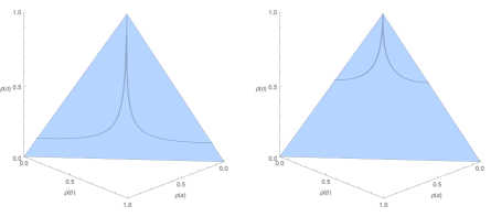
Figure 4: Binary choice probability distributions that are compatible with the reciprocal-differences model for a given value of $\lambda$ (the latter is higher in the right graph).

Figure 4 depicts two classes of binary choice probability distributions that are compatible with the reciprocal-differences model for different values of $\lambda$. It demonstrates how the probability of deferring choice increases as the two active-choice alternatives become more similar in their appeal. It also shows that, other things equal, a higher value of $\lambda$ means a lower permissible maximum choice probability for the active-choice alternatives.

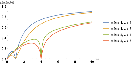
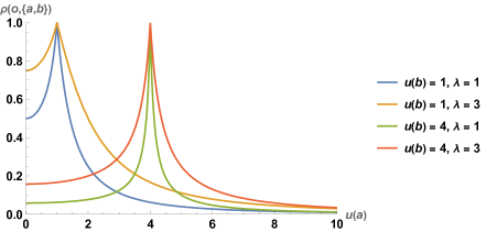
Figure 5: Comparative statics in the reciprocal utility differences model when one of the two alternatives becomes more attractive.

Figure 5 on the other hand is the analogue of Figure 3 for binary-choice comparative statics in the reciprocal-differences model. It shows the behaviour of $\rho(a,\{a,b\})$ and $\rho(o,\{a,b\})$ as the attractiveness of $a$ changes while that of $b$ is held fixed, for different values of the sensitivity parameter $\lambda$. Unlike in the quadratic-logit model, the probability $\rho(a,\{a,b\})$ attains a local maximum as $u(a)$ lies in the sub-interval $\big{(}0,u(b)\bigr{)}$; it goes to zero (and $\rho(o,\{a,b\})$ goes to one) as $u(a)\rightarrow u(b)$; and it increases monotonically once $u(a)$ has surpassed $u(b)$ and continues to increase. In addition, the local maximum and rate of increase in $\rho(a,\{a,b\})$ as $a$ becomes more appealing are higher for lower $\lambda$, as expected.

We further note that, in addition to the DDM, the reciprocal-differences model and the generalization of this model that we study in the Online Supplementary Appendix are related to Fechnerian representations of binary random choice models without an outside option Falmagne (2002, p. 118); Fudenberg et al. (2015, p. 2381). These predict that the choice probability of $a$ at menu $\{a,b\}$ is a strictly increasing function of the value difference between $a$ and $b$, which in turn implies that, as with any $\rho=(u,\lambda)$ model, alternative $a$ is more likely to be chosen when its utility difference from $b$ increases, other things equal.

5     Explanations of Choice-Deferral Phenomena

We proceed with an illustration of how an otherwise unstructured decision-conflict logit model and the more structured such models of the previous two sections in particular help explain some intuitive and empirically documented choice-deferral phenomena.

Since, as was discussed in Section 2.2, it is not generally true that deferring becomes more likely as menus expand even for monotonic decision-conflict logit models, it is naturally of interest to understand when exactly such behaviour is to be expected in this environment. The general idea in answering this question is that, even if decision difficulty increases in absolute terms when new alternatives are introduced, when these new alternatives are sufficiently better than the pre-existing ones their added value will offset the elevated decision cost and will ultimately result in a higher probability of making an active choice at the larger menu. To state this more formally we will abuse notation slightly by letting

$$u(S) := \sum_{s\in S}u(s)$$ (14)

stand for the total Luce utility in menu $S\in{\mathcal{M}}$.

Observation 3 (“Roller-Coaster” Choice-Deferral Effects)

If $\rho=(u,D)$ is a decision-conflict logit, then for any $A,B\in{\mathcal{M}}$ such that $A\supset B$:

$$\rho(o,A)\leq\rho(o,B) \Longleftrightarrow \underbrace{\frac{D(A)-D(B)}{D(B)}}_{\text{\shortstack{marginal cost\\ from menu expansion}}}\leq\underbrace{\frac{u(A)-u(B)}{u(B)}}_{\text{\shortstack{marginal benefit\\ from menu expansion}}}.$$ (15)

This eloquent equivalence clarifies that the choice probability of opting out will decrease following menu expansion if and only if the marginal benefit of this expansion, as measured by the percentage increase in total utility, exceeds its marginal cost, as measured by the percentage increase in decision complexity. This is a distinctive property of decision-conflict logit models. It clarifies that they do not belong to the random-utility class (Block and Marschak, 1960; Apesteguia et al., 2017) with an outside option, and enables them to explain simply the non-monotonic and dominance-driven effect that menu expansion has been known to exert on the probability of deferring (Scheibehenne et al., 2010; Chernev et al., 2015), which we will refer to as “roller-coaster choice overload” effect.

Indeed, citing several studies in consumer psychology, the meta-analysis in Chernev et al. (2015) notes that “it has been shown that consumers are more likely to make a purchase from an assortment when it contains a dominant option than when such an option is absent” (p. 338). This finding is important for the interpretation and policy responses to choice-overload phenomena of the kind that were first reported in Iyengar and Lepper (2000). To our knowledge, the decision-conflict logit is the first random-choice model that predicts this dominance-driven emergence and disappearance of choice-overload effects, and it does so without imposing any undesirability or inattention constraints. Table 1 illustrates an example such effect that is predicted by the quadratic logit model (see also Figure C1(b)).

Table 1: An example “roller-coaster choice-overload” effect generated by the quadratic logit model.

Option	$\widehat{u}$	$\rho(\cdot,\{a,b\})$	$\rho(\cdot,\{a,b,c\})$	$\rho(\cdot,\{a,b,c,d\})$
$a$	10	0.980	0.250	0.007
$b$	0.1	0.001	0.000	0.000
$c$	9.9	$-$	0.245	0.007
$d$	100	$-$	$-$	0.694
$o$	$-$	0.019	$\nearrow$  0.505  $\searrow$	0.292

Observation 4 (Similarity-Driven Deferral)

For any $\rho=(u,\lambda)$ and any $a,b\in X$, $\rho(o,\{a,b\})$ is strictly decreasing in $|u(a)-u(b)|$.

This prediction –illustrated in Figure C2(a)– and that model’s mechanism for generating it are consistent with findings and arguments from the consumer-psychology literature that were given in Dhar (1997), Sela et al. (2009) and Scheibehenne et al. (2010), for example. The latter authors, in particular, noted that as the most attractive feasible options become more similar when new items are added to a menu, it can become more difficult for the decision maker to justify the choice of any particular option, which in turn would increase the likelihood of choice deferral. In the same direction but focusing on response times rather than deferral decisions, Bhatia and Mullett (2018) recently reported evidence to suggest that choice between similarly attractive options is significantly correlated with longer response times, in line also with the predictions of the DDM discussed earlier.

Observation 5 (Absolute & Relative Attractiveness Effects)

For any $\rho=(u,\lambda)$ and any alternatives $a,b,c,d\in X$ such that $u(a)>u(b)$ and $u(c)>u(d)$, it holds that

$$\rho(o,\{c,d\}) > \rho(o,\{a,b\})$$

whenever

$$u(a)-u(b)>u(c)-u(d) u(a)+u(b)=u(c)+u(d),$$ and

or

$$u(a)+u(b)>u(c)+u(d) u(a)-u(b)=u(c)-u(d).$$ and (17)

Condition (5) clarifies that opting out is more likely at $\{c,d\}$ than it is at $\{a,b\}$ if the two binary menus have the same total value but the utility difference in $\{a,b\}$ is greater. The model therefore predicts the “relative attractiveness” effect, depicted in Figure C2-(b), which is defined by this phenomenon (Dhar, 1997; Bhatia and Mullett, 2016). Condition (17) on the other hand clarifies that opting out is more likely at $\{c,d\}$ if the utility differences are the same in both menus but total utility is higher at $\{a,b\}$. The prediction of this “absolute attractiveness” effect (Tversky and Shafir, 1992; White et al., 2015; Bhatia and Mullett, 2016), illustrated in Figure C2-(c), is also intuitive: as the menu becomes more valuable the agent finds making an active choice more appealing, other things equal. In keeping with the analogy between the reciprocal-differences model and DDM that we drew in the previous section, we further note that this prediction of the model is also supported by experimental evidence recently reported in Steverson et al. (2019) and Shevlin et al. (2022) which suggest that faster and more accurate binary decisions are made between high-value options compared to low-value ones.

6     Applications

6.1     Proliferation, Simplicity Seeking, and Optimal Choice Architecture

In addition to choice-deferring behaviours, the presence of many alternatives in a menu is also known to be associated with other impairments in decision-making quality. Notably, Iyengar and Kamenica (2010) have shown that when experimental subjects have to make choices from a large menu of lotteries, they tend to choose ones that are simple in the sense that they feature relatively few possible outcomes that occur with positive probability. In this section we show how incorporating into the decision-conflict logit insights from the recent decision-theoretic literature on preferences for simple lotteries helps explain some key findings in Iyengar and Kamenica (2010), and additionally generates novel testable predictions concerning the choice of simple lotteries vs the decision to defer/avoid choice in large menus.

Let $Z\subset\mathbb{R}$ be a finite set of monetary outcomes, and let the grand choice set $X$ now be a finite set of lotteries over $Z$. In what follows we consider a simple $(u,D)$ model on this $X$ by: (i) adopting a special case of the preference-for-simplicity utility representation proposed and analysed in Puri (2020); and (ii) linking the decision maker’s aversion to multiple-outcome lotteries with an increased difficulty in comparing such lotteries. Specifically, for $p$ and $q$ in $X$ we let

$$u(p) := \mathbb{E}_{p}(z)-\alpha|support(p)|,$$ (18)

$$D(\{p,q\}) := \beta\big{(}|support(p)|+|support(q)|\bigr{)},$$ (19)

where $\alpha\geq 0$ and $\beta\geq 0$ are the decision maker’s complexity-aversion and comparison-difficulty parameters, respectively. Thus, other things equal, the agent dislikes lotteries with many non-zero probability outcomes and, in addition, finds it difficult to compare such lotteries. When $\beta=0$ the model reduces to the standard logit without an outside option that features (6) and (18). When $\alpha=0$ and $\beta>0$, the agent’s complexity aversion enters the model by altering the difficulty in comparing lotteries with different supports. The more general case where $\alpha$ and $\beta$ are distinct and strictly positive portrays the agent as being challenged by complexity both when evaluating each lottery in isolation and when comparing different lotteries. Such a specification predicts high market shares for simple lotteries and/or the outside option, depending on the specific parameter values. Under $D$-additivity in the sense of (12), which we also assume to close the model, it also exhibits a particular symmetry with respect to its parameter values: the special case where $\alpha=\beta>0$ leads to a cancellation of the complexity-aversion terms in (18)-(19) and, as with the case where $\beta=0$, reduces the model to the standard logit without an outside option.

First, to explain the findings in Iyengar and Kamenica (2010) where experimental subjects could not avoid/delay choice, we study the first special case of interest where $\beta=0$. We focus on the second experiment from that study. There, one group of subjects were asked to choose from the set that contained the 11 lotteries shown in Table 2. Ten of these lotteries featured up to 6 distinct monetary outcomes, while one (the first item in the table) had only 2 such outcomes. Other groups of subjects were asked to choose from various subsets of 3 lotteries instead, all of which also included the simple lottery. Iyengar and Kamenica (2010) found that 57% of subjects in the first group chose the simple lottery, whereas only 16% did so in the second class of groups ($p<0.001$).

Table 2: The 11 lotteries in the second experiment of Iyengar and Kamenica (2010).

Probability	$\dfrac{1}{6}$	$\dfrac{1}{6}$	$\dfrac{1}{6}$	$\dfrac{1}{6}$	$\dfrac{1}{6}$	$\dfrac{1}{6}$
Lottery
1	$0.00	$0.00	$0.00	$10.00	$10.00	$10.00
2	$1.50	$9.25	$8.75	$7.00	$0.75	$1.25
3	$4.25	$5.50	$9.75	$8.50	$0.00	$0.75
4	$1.00	$2.00	$6.75	$7.50	$5.75	$4.75
5	$5.50	$1.00	$0.75	$6.50	$7.50	$6.75
6	$0.00	$0.00	$8.75	$2.75	$9.75	$8.00
7	$9.75	$3.00	$7.00	$6.50	$0.50	$1.50
8	$9.50	$1.50	$1.50	$2.50	$3.25	$10.00
9	$5.50	$8.50	$3.25	$0.00	$8.50	$2.50
10	$9.25	$7.75	$3.75	$2.00	$3.25	$2.00
11	$1.25	$4.50	$8.50	$8.75	$4.50	$0.75

Interestingly, the basic preference-for-simplicity logit defined by (6) and (18) almost exactly matches both the market share of the simple lottery in the extended menu (predicted share: 0.576) and that of the second-simplest and second most demanded lottery 8 in Table 2 when the parameter $\alpha=0.77$ (16% actual share vs 14.3% predicted). On the other hand, the model predicts similar market shares for the equally simple lotteries 6 and 8 even though the actual share of the former was very low despite its slightly higher expected value, which is in turn presumably caused by this lottery’s relatively high probability of a zero reward. Replacing the risk-neutral specification in (18) with a risk-averse one improves the model’s fit in this respect too.

We now turn to the case where $\beta>0$ in (19) so as to explore the model’s predictions on that same 11-lottery menu from Iyengar and Kamenica (2010) in the counterfactual case where opting out was also possible.

Table 3: Predicted shares of the two simplest/most demanded lotteries when delaying choice is also possible and $\alpha$ is fixed at its forced-choice optimal level of 0.77.

$\beta$	$\rho(1)$	$\rho(8)$	$\rho(o)$
0.001	0.522	0.129	0.092
0.005	0.381	0.094	0.336
0.01	0.285	0.070	0.503
0.05	0.094	0.023	0.835
0.1	0.051	0.012	0.910

Holding constant the value of $\alpha$ at its optimal level of 0.77 that corresponds to the forced-choice experimental dataset, Table 3 shows how the model’s trade-off between simplicity-seeking and deferring behaviour is resolved at different values of $\beta$. Considering also the empirical findings from Iyengar and Kamenica (2010), the choice-overload literature, and the absence of a clearly superior lottery in this extended menu, the table clarifies that the intuitive testable predictions of the model when opting out is also feasible are generated when $\beta\in[0.001,0.01]$, with lower values of this comparison-difficulty parameter naturally favouring the simple lottery(ies) relative to the outside option, and with higher values doing the opposite.

This counterfactual analysis is clearly relevant for choice architecture. Indeed, in many real-world environments such as investment, insurance or consumer decision-making, people are often faced with similarly abounding active-choice options that are feasible to them and at the same time are not forced to choose any. When it is normatively appealing for the decision maker to make an active choice sooner rather than later in such situations but this is difficult because of option/menu complexity and/or comparison difficulty, the combined empirical evidence for simplicity-seeking and choice-deferring behaviours point to the importance of understanding how simple the simplest options in the menu must be in order for them to minimize the probability of choice avoidance/delay. The study of stochastic-choice models such as the simple one presented in this section could be useful in this regard.

6.2     The Conditional Quadratic Logit and Discrete-Choice Estimation

We now show how the assumptions and argument that underpin the conditional-logit formulation of Luce’s (1959) model without an outside option can be modified to arrive at a similar discrete-choice version of the quadratic logit. Without loss of generality we will focus on the grand choice set $X$, and write $X:=\{a_{1},\ldots,a_{k}\}$.

We start by recalling and breaking down the baseline assumptions of the conditional-logit formulation of (6) as follows:
1. Additive and linear random utility [structural assumption]: there is some function $u:X\rightarrow\mathbb{R}$ such that

$$u(a_{i}) = \beta\cdot x_{i}+\epsilon_{i},$$ (20)

where $\epsilon_{i}$ is an additive error term (see also below) and $x_{i}$, $\beta$ are, respectively, vectors of product/consumer characteristics and coefficients capturing their relative importance.
2. Random utility maximization [behavioural assumption]: for all $a_{i}\in X$,

$$\rho(a_{i},X) = Pr\big{(}u(a_{i})\geq u(a_{j})\text{ for all }j\leq k\bigr{)}.$$ (21)

3. Gumbel-distributed noise [distributional assumption]: the error term $\epsilon_{i}$ is independently and identically distributed across $i$ according to the standard Gumbel density

$$f(\epsilon_{i}) = e^{-\epsilon_{i}}e^{-e^{-\epsilon_{i}}}.$$ (22)

As Holman and Marley [see Luce and Suppes (1965) and Anderson et al. (1992)] and McFadden (1973) showed, these assumptions jointly imply the analytically convenient and famous form

$$\rho(a_{i},X) = \frac{e^{\beta\cdot x_{i}}}{\sum\limits_{j=1}^{k}e^{\beta\cdot x_{j}}}.$$ (23)

Let us now examine how the premises and conclusion of this conditional-logit model are affected and can be modified when we assume that the decision maker uses the single but noisy utility criterion captured by $u$ to sample the values of the alternatives in $X$ twice, as per the predictions of the quadratic logit. To this end we note first that maintaining the additive and linear utility assumption implies that at the end of the second round of sampling the individual has perceived two values for each alternative $a_{i}\in X$,

$$u^{1}(a_{i}) = \beta\cdot x_{i}+\epsilon_{i}^{1},$$

$$u^{2}(a_{i}) = \beta\cdot x_{i}+\epsilon_{i}^{2}.$$

These generally distinct values across the two rounds will vary according to the distribution of $\epsilon_{i}$. Such multiplicity of value realizations in turn implies that each alternative $a_{i}\in X$ is ultimately associated with a vector of values $\big{(}u^{1}(a_{i}),u^{2}(a_{i})\bigr{)}$. With utility now being vector-valued, however, the utility-maximization behavioural assumption that underpins (23) is no longer applicable in an obvious way. To break this impasse we assume that the random utility maximization behavioural assumption is replaced by a dominance assumption whereby

$$\rho(a_{i},X) = Pr\big{(}u^{l}(a_{i})\geq u^{l}(a_{j})\text{ for all }j\leq k\text{ and for all }l=1,2\bigr{)}.$$ (24)

Turning, finally, to the modification of the distributional assumption in the discrete-choice formulation of the standard logit without an outside option, to make it operational in the quadratic-logit framework we assume that the random errors $\epsilon_{i}^{1}$ and $\epsilon_{i}^{2}$ are independent across all alternatives $i\leq k$ and across the two sampling rounds $l\leq 2$.

With these assumptions in place we can now write

$$\rho(a_{i},X) = Pr(u^{1}(a_{i})\geq u^{1}(a_{j})\;\forall\;j\neq i)\cdot Pr(u^{2}(a_{i})\geq u^{2}(a_{j})\;\forall\;j\neq i)$$ (25)

$$= Pr(\beta\cdot x_{i}+\epsilon_{i}^{1}\geq\beta\cdot x_{j}+\epsilon_{j}^{1}\;\forall\;j\neq i)\cdot Pr(\beta\cdot x_{i}+\epsilon_{i}^{2}\geq\beta\cdot x_{j}+\epsilon_{j}^{2}\;\forall\;j\neq i)$$

$$= Pr(\epsilon_{j}^{1}\leq\beta\cdot x_{i}+\epsilon_{i}^{1}-\beta\cdot x_{j}\;\forall\;j\neq i)\cdot Pr(\epsilon_{j}^{2}\leq\beta\cdot x_{i}+\epsilon_{i}^{2}-\beta\cdot x_{j}\;\forall\;j\neq i)$$

$$= \begin{split}\int_{-\infty}^{\infty}\left(\prod_{j\neq i}e^{-e^{-(\epsilon_{i}^{1}+\beta\cdot x_{i}-\beta\cdot x_{j})}}\right)e^{-\epsilon_{i}^{1}}e^{-e^{-\epsilon_{i}^{1}}}d\epsilon\\ \times\int_{-\infty}^{\infty}\left(\prod_{j\neq i}e^{-e^{-(\epsilon_{i}^{2}+\beta\cdot x_{i}-\beta\cdot x_{j})}}\right)e^{-\epsilon_{i}^{2}}e^{-e^{-\epsilon_{i}^{2}}}d\epsilon\end{split}$$

$$= \left(\frac{e^{\beta\cdot x_{i}}}{\sum\limits_{j=1}^{k}e^{\beta\cdot x_{j}}}\right)^{2},$$

where each integral is $k$-dimensional, the first and second steps make use of the above behavioural, distributional and independence assumptions on $\epsilon_{i}^{l}$, while the last step follows from the derivation of the conditional logit model [see, for example, Train (2009, pp. 74-75)].

An important difference between the conditional logit with an outside option and the conditional quadratic logit in (25) is that in the former case the modeller specifies the utility of that option exogenously (see Anderson et al., 1992; Hensher et al., 2015), whereas in the latter case this utility emerges endogenously and is estimated from the available data. Indeed, upon rewriting (25) as

$$\rho(a_{i},X) = \frac{e^{2\beta\cdot x_{i}}}{\sum\limits_{j=1}^{k}e^{2\beta\cdot x_{j}}+2\sum\limits_{i\neq j}e^{\beta\cdot(x_{i}+x_{j})}},$$

we observe that

$$u(a_{i}) \equiv e^{2\beta\cdot x_{i}},$$

$$D(X) \equiv 2\sum_{i\neq j}e^{\beta\cdot(x_{i}+x_{j})}.$$

Following McFadden (1973) and the ensuing literature, the vector $\beta$ in (25) can be estimated by minimizing the log-likelihood function that emerges from this model. By construction, however, all observations where the decision maker(s) avoided/delayed choice by selecting $o$ are automatically dropped out by the log-likelihood function. This results in the conditional quadratic logit estimator of $\beta$ to coincide with the estimator that comes from the standard conditional logit without an outside option in the restricted subset of the original dataset where all $o$ choice observations are removed. However, the two models’ predictions on the original dataset obviously differ, as do the predictions between (25) and the conditional logit with an outside option once a utility value is exogenously fixed for $o$.

For practical purposes, the added value of the conditional quadratic logit in empirical estimation will be seen when the researcher wishes to analyse discrete non-forced choice data with menu variation and when they suspect that the no-choice outside option in such data is often selected because of the decision makers’ inability to find and choose a most preferred alternative. In situations like this the analyst can then quantify the model’s added value by comparing, for example, its average mean-squared error (MSE) across all available menus to the MSE corresponding to the conditional or nested logit with an outside option, or by comparing the MSEs of these models that are based on suitable parameter averages across the relevant menus.

6.3     Price-Quality Competition with Quadratic-Logit Market Shares

Piccione and Spiegler (2012), Spiegler (2015), Bachi and Spiegler (2018) and Gerasimou and Papi (2018) have recently suggested distinct approaches to study oligopolistic markets when consumers may face comparison difficulties or are possibly choice-overloaded. In this section we contribute to this literature by illustrating the potential usefulness of the quadratic logit in the analysis of such markets when products are differentiated in price and quality and consumers can opt out due to decision difficulty.

To this end, we consider a market where two profit-maximizing firms compete for a single consumer (equivalently, a unit mass of consumers) by offering a product that is differentiated in quality, $q_{i}$, and price, $p_{i}$. Producing a product of quality $q_{i}$ costs $q_{i}$ to firm $i=1,2$, while $0\leq q_{i}\leq p_{i}\leq I$ and $I>0$ denotes consumer income. Furthermore, utility from product $(q_{i},p_{i})$ coincides with that product’s quality-price ratio:

$$u(q_{i},p_{i}) = \frac{q_{i}}{p_{i}}.$$ (26)

This assumption further implies

$$u(q_{i},p_{i}) \in [0,1]$$ (27)

for all $(q_{i},p_{i})$. Such a “value-for-money” specification imposes intuitive positive and negative dependences of utility on quality and price, respectively, with the former being linear and the latter strictly convex. Moreover, while identifying utility with quality-price ratios as in (26) rather than with quality-price differences $q_{i}-p_{i}$ appears to be a novel modelling assumption, it is consistent with some central implications of the influential behavioural choice model in Bordallo et al. (2013) concerning consumer preferences for high quality-price ratio products, even though that model starts from very different primitives and features a quality-price difference utility function instead.

The two firms choose their products’ quality and price levels simultaneously and under complete information. The market share of product $(q_{i},p_{i})$ at menu/strategy profile $\big{(}(q_{1},p_{1}),(q_{2},p_{2})\bigr{)}$ is determined by the baseline logit model

$$\rho\big{(}(q_{i},p_{i}),\{(q_{j},p_{j})\}_{j=1}^{2}\bigr{)} = \displaystyle\frac{\displaystyle\frac{q_{i}}{p_{i}}}{\displaystyle\frac{q_{i}}{p_{i}}+\displaystyle\frac{q_{j}}{p_{j}}}$$

when there is no decision difficulty, and by the quadratic logit model

$$\rho\big{(}(q_{i},p_{i}),\{(q_{j},p_{j})\}_{j=1}^{2}\bigr{)} = \displaystyle\left(\displaystyle\frac{\displaystyle\frac{q_{i}}{p_{i}}}{\displaystyle\frac{q_{i}}{p_{i}}+\displaystyle\frac{q_{j}}{p_{j}}}\right)^{2}$$

when there is.

Letting the index variable $s\in\{1,2\}$ capture these two possibilities, the above assumptions imply that each firm $i=1,2$ solves

$$\max_{0\leq q_{i}\leq p_{i}\leq I}\pi_{i}(q_{i},p_{i}) := \left(\frac{\displaystyle\frac{q_{i}}{p_{i}}}{\displaystyle\frac{q_{i}}{p_{i}}+\displaystyle\frac{q_{j}}{p_{j}}}\right)^{s}\cdot(p_{i}-q_{i}).$$ (28)

The strategic trade-off in this model, which applies both when $s=1$ and $s=2$, is that each firm wishes to increase its quality/price ratio in order to expand its market share, while at the same time also wishing to decrease it in order to enlarge its profit markup.

Turning to consumer welfare, taking into account that decision conflict can potentially drive the consumer out of the market altogether, and that -by A3- this would be undesirable, we consider a utilitarian welfare measure that weighs the possible utility levels at a given strategy profile by the probabilities that these utilities will actually be realized at that profile. We formalize this with the utilitarian consumer welfare function $W:\mathbb{R}^{4}_{++}\rightarrow[0,1]$ that is defined by

$$W\big{(}(q_{i},p_{i}),(q_{j},p_{j})\bigr{)} = \rho((q_{i},p_{i}),\{(q_{j},p_{j})\}_{j=1}^{2})\cdot u(q_{i},p_{i})+\rho((q_{j},p_{j}),\{(q_{j},p_{j})\}_{j=1}^{2})\cdot u(q_{j},p_{j}).$$

This welfare indicator may be particularly relevant in cases where consumer surplus is equilibrium-invariant, as will turn out to be the case in the present environment.

Proposition 4

The logit equilibrium is $(q_{1}^{*},p_{1}^{*})=(q_{2}^{*},p_{2}^{*})=(\frac{I}{3},I)$, and features an expected profit of $\frac{I}{3}$ for each firm and a consumer welfare level of $\frac{1}{3}$ with certainty.

The quadratic-logit equilibrium is $(q_{1}^{**},p_{1}^{**})=(q_{2}^{**},p_{2}^{**})=(\frac{I}{2},I)$, and features an expected profit of $\frac{I}{8}$ for each firm, the consumer being equally likely to defer or choose a product, and a consumer welfare level of $\frac{1}{4}$ in expectation.

Thus, when the consumer makes decisions as if they had previously resampled the available alternatives twice as per the quadratic logit model, each firm increases its quality level by 50% in equilibrium relative to the baseline case where there is no hesitation/resampling. An intuitive interpretation of this fact is that decision conflict inevitably introduces a third “competitor” into the market: the outside option. The quadratic logit predicts that the choice probability of the outside option goes down as the utility of one of the two products is unilaterally increased, while the choice probability of the comparatively more appealing product simultaneously goes up during the process. This in turn creates incentives for each firm to unilaterally increase its quality level relative to the baseline logit case. But since increasing quality is costly, the above-mentioned strategic trade-off that is embedded in each firm’s profit function eventually kicks in and halts this increase at the $\frac{I}{2}$ symmetric-equilibrium level.

Notably, while consumer surplus is zero in both equilibria because each firm’s profits turn out to be strictly increasing in its product’s price, consumer welfare changes in an interesting way. In particular, despite the 50% increase in the attainable utility level in equilibrium once firms best-respond to the consumer’s hesitation and resampling, welfare goes down by 25%. This decrease is caused by the fact that in the quadratic logit with two equally attractive products the consumer is equally likely to defer or make an active choice (Observation 2) and, conditional on the latter, also equally likely to choose either of the two available products. The implication of this fact in the present environment is that the higher utility level that the consumer receives in expectation under the equilibrium with decision conflict is not sufficiently high to offset the lower utility level that they receive with certainty under the equilibrium without conflict.

The firms’ profits, finally, are decreased by 62.5% when there is decision difficulty relative to the case where there is not. This large decrease is intuitive and contributed by the halved probability of the consumer choosing either product, as well as by the 50% reduction in the firms’ profit margins that is brought about by the improvement in quality.

7     Related Literature

Standard discrete choice models with an outside option that are based on random-utility maximization that include such an option treat it just like any other alternative, and predict that it is chosen when its utility is higher than that of all feasible active-choice options. Anderson et al. (1992), Hensher et al. (2015), for example, are textbook references that discuss this approach in detail. Starting with Manzini and Mariotti (2014), moreover, several random choice models of limited attention that are logically distinct from the modelling framework proposed in this paper have included an outside option as a model-closing assumption that requires this option to be chosen when no attention is paid to any of the feasible market alternatives. Because of this assumption, deferring becomes less likely in these models as menus become bigger. Horan (2019) recently clarified, however, how the deferral option can be removed from these models without affecting their general features and primary purpose, which is to explain active-choice decision making subject to cognitive/attention constraints.

Also distinct from the modelling framework of this paper in their motivations, components and predictions are the perception-adjusted Luce model in Echenique et al. (2018) and the focal Luce model in Kovach and Tserenjigmid (2022b). In the former, choice probabilities are influenced by the alternatives’ position in a priority ordering. As the authors showed, the choice probability of the outside option is weakly higher in that model than what it would have been in the corresponding baseline Luce model with an outside option, as the utility of that option is the sum of a menu-independent and a menu-dependent part. The ingredients of the focal Luce in Kovach and Tserenjigmid (2022b) on the other hand comprise: (i) a menu-independent utility function over alternatives; (ii) a menu-dependent focus function that assigns a consideration set to every menu; (iii) a menu-dependent focality bias function that gives a “utility boost” to alternatives in the consideration set. This is more closely related to the present paper’s contribution but is still logically and interpretatively distinct from it. In Appendix B we illustrate how the focal Luce model that includes the outside option as part of the choice domain and treats it like any other alternative coincides with a class of Luce models with a menu-dependent utility of this option that does not contain the decision-conflict logit class but does contain the corresponding Luce model described in (5).

We note further that the nested logit model (Train, 2009, Chapter 4), recently axiomatized and generalized in Kovach and Tserenjigmid (2022a), is also known to allow for the inclusion of an outside option where one nest comprises all active-choice alternatives while the second only contains that special option. This specification too assigns a menu-independent utility to the outside option and is therefore not suitable for explaining the kinds of behaviour that motivate the decision-conflict logit class. On the other hand, each of the perception-adjusted, focal and nested Luce models allow for violations of the (active-choice) Luce axiom and are therefore more suitable for explaining context-dependent choice effects that involve reversals between active-choice alternatives.

Working within forced- and non-forced general deterministic choice environments, respectively, Frick (2016) and Gerasimou (2018, Section 4) study threshold models that also predict choice-overload effects by means of menu complexity functions that are monotonic in set inclusion and lead to increased levels of choice inconsistency and choice deferrals, respectively, as menus expand. Buturak and Evren (2017), on the other hand, takes menus of lotteries as the primitive and models the decision maker as making an active choice at a menu if and only if the Sarver (2008) regret-inclusive expected utility of the most preferred feasible alternative exceeds the menu-independent cut-off utility of the outside option. Thus, unlike the general and special decision-conflict logit models analysed in this paper, the above cannot explain, for example, the observed dominance-driven “roller-coaster choice overload” effect of Section 5. On the other hand, the deferral-permitting deterministic model of dominant choice with incomplete preferences in Gerasimou (2018, Section 2) does predict such effects in a non-random setting but is not suitable for thinking about absolute and relative attractiveness effects, for example.

8     Concluding Remarks

Understanding the “easy” and “hard” parts of people’s preference comparisons as these are revealed by their active-choice or choice-avoidance/delay decisions is important methodologically and also for practical applications such as effective choice architecture. The present paper contributes in this respect by introducing the tractable class of decision-conflict logit models and analysing two intuitively structured special cases thereof. These random-choice models assume that people can avoid/delay making an active choice and are more likely to select the choice-deferral outside option when it is harder for them to identify a best alternative from those available to them. This prediction is supported empirically and differs from the predictions of existing models where the outside option is chosen due to the undesirability of all feasible alternatives, limited attention, or other sources of bounded-rational behaviour. Thus, the class of decision-conflict logit models that we introduce and study in this paper complement existing ones in empirically relevant and, as we demonstrated, economically applicable ways.

In conjunction with the insights from the relevant theoretical and experimental/empirical decision-making literature, our analysis suggests that decision-conflict models can help theoretical and applied economists think formally and perhaps more realistically about (non-)strategic situations where decision makers: (i) are presented sufficiently small menus, so that limited-attention considerations are not pertinent; (ii) consider all feasible active-choice alternatives to be desirable/good enough, so that any one of them would be expected to be chosen if it were the only feasible item; (iii) find it difficult to compare these alternatives due to their complexity or due to potentially non-trivial trade-offs these generate (e.g. treatment efficacy vs safety); and (iv) are not forced to make an active choice.

We note, finally, that an important limitation of the hereby proposed modelling framework is that it relies upon a version of the Luce/IIA axiom which, although weaker than its standard version, is nevertheless demanding and likely to be descriptively challenged. Future extensions of decision-conflict logit models that relax this assumption further while retaining discipline and tractability would therefore be particularly welcome. In addition to the phenomena discussed in Section 5, such extensions could also aim to explain the intuitive strengthening of well-known context-dependent choice effects that have been observed when active decisions are not forced upon individuals, such as those reported, for example, in Dhar and Simonson (2003).

Appendix A: Proofs

Proof of Proposition 1.

In the main text. $\blacksquare$

Proof of Corollary 1.

In the main text. $\blacksquare$

Proof of Proposition 2.

Let $X:=\{a_{1},\ldots,a_{k}\}$ and suppose $\rho=(u,D)$ is a decision-conflict logit on $X$. Consistent with (3), and without loss of generality, we may let

$$u(a_{i}):=\frac{\rho(a_{i},X)}{\rho(a_{1},X)}.$$

Note that $\rho$ has the quadratic-logit property at the binary menus of $X$ iff there is a vector $\big{(}\widehat{u}(a_{1}),\ldots,\widehat{u}(a_{k})\bigr{)}$ that solves the system

$$\left(\begin{array}[]{c}\widehat{u}(a_{1})^{2}\\ \widehat{u}(a_{2})^{2}\\ \vdots\\ \widehat{u}(a_{k})^{2}\\ 2\widehat{u}(a_{1})\widehat{u}(a_{2})\\ 2\widehat{u}(a_{1})\widehat{u}(a_{3})\\ \vdots\\ 2\widehat{u}(a_{1})\widehat{u}(a_{k})\\ 2\widehat{u}(a_{2})\widehat{u}(a_{3})\\ \vdots\\ 2\widehat{u}(a_{k-1})\widehat{u}(a_{k})\end{array}\right)=\left(\begin{array}[]{c}u(a_{1})\\ u(a_{2})\\ \vdots\\ u(a_{k})\\ D(\{a_{1},a_{2}\})\\ D(\{a_{1},a_{3}\})\\ \vdots\\ D(\{a_{1},a_{k}\})\\ D(\{a_{2},a_{3}\})\\ \vdots\\ D(\{a_{k-1},a_{k}\})\end{array}\right)\equiv\left(\begin{array}[]{c}1\\ \frac{\rho(a_{2},X)}{\rho(a_{1},X)}\\ \vdots\\ \frac{\rho(a_{k},X)}{\rho(a_{1},X)}\\ \frac{\rho(o,\{a_{1},a_{2}\})}{\rho(a_{1},\{a_{1},a_{2}\})}\\ \frac{\rho(o,\{a_{1},a_{3}\})}{\rho(a_{1},\{a_{1},a_{3}\})}\\ \vdots\\ \frac{\rho(o,\{a_{1},a_{3}\})}{\rho(a_{1},\{a_{1},a_{k}\})}\\ \frac{\rho(o,\{a_{2},a_{3}\})}{\rho(a_{2},\{a_{2},a_{3}\})}\frac{\rho(a_{2},X)}{\rho(a_{1},X)}\\ \vdots\\ \frac{\rho(o,\{a_{k-1},a_{k}\})}{\rho(a_{k-1},\{a_{k-1},a_{k}\})}\frac{\rho(a_{k-1},X)}{\rho(a_{1},X)}\end{array}\right),$$ (29)

where we’ve simplified the subset of equations that pertain to $D$ in the last column vector of (29) by making a particular use of the fact that

$$\frac{\rho(A,X)}{\rho(A,A)} = \frac{\rho(a,X)}{\rho(a,A)}\;\;\text{ for any }a\in A\in{\mathcal{M}},$$ (30)

which, in turn, is a straightforward implication of A2.

Next, we observe that (29) reduces to

$$u(a_{1}) = 1,$$

$$u(a_{i}) = \frac{D(\{a_{1},a_{i}\})^{2}}{4},\;1\neq i\leq k,$$

which in turn imply

$$\widehat{u}(a_{1}) = 1,$$ (31)

$$\widehat{u}(a_{i}) = \frac{D(\{a_{1},a_{i}\})}{2},\;1\neq i\leq k.$$ (32)

By (29) and (32) we have

$$D(\{a_{1},a_{j}\}) = \frac{\rho(o,\{a_{1},a_{j}\})}{\rho(a_{1},\{a_{1},a_{j}\})}$$ (33)

for all $j\neq 1$. By (33) and the above we also get

$$\widehat{u}(a_{j}) = \frac{1}{2}\frac{\rho(o,\{a_{1},a_{j}\})}{\rho(a_{1},\{a_{1},a_{j}\})}$$ (34)

for all such $j$. By (29) and A2, moreover, we also have

$$\widehat{u}(a_{j})^{2} = \frac{\rho(a_{j},X)}{\rho(a_{1},X)}$$ (35)

$$= \frac{\rho(a_{j},\{a_{1},a_{j}\})}{\rho(a_{1},\{a_{1},a_{j}\})}.$$

Therefore, by (34) and (35), consistency of (29) is achieved iff

$$\frac{1}{4}\left(\frac{\rho(o,\{a_{1},a_{j}\})}{\rho(a_{1},\{a_{1},a_{j}\})}\right)^{2} = \frac{\rho(a_{j},\{a_{1},a_{j}\})}{\rho(a_{1},\{a_{1},a_{j}\})},$$

which is easily seen to be equivalent to A4. $\blacksquare$

Proof of Proposition 3.

Let $\rho=(u,D)$ be a decision-conflict logit. By (3) and (4), there are $\alpha>0$ and $z\in X$ such that

$$D(A) = \alpha\frac{\rho(o,A)}{1-\rho(o,A)}\cdot\sum_{b\in A}\frac{\rho(b,X)}{\rho(z,X)}$$ (36)

$$= \alpha\frac{\rho(A,X)}{\rho(z,X)}\cdot\frac{\rho(o,A)}{1-\rho(o,A)},$$

and

$$D(\{a,b\}) = \alpha\frac{\rho(\{a,b\},X)}{\rho(z,X)}\cdot\frac{\rho(o,\{a,b\})}{1-\rho(o,\{a,b\})}.$$ (37)

Now recall that A5 is satisfied iff, for all $A,B\in{\mathcal{M}}$ with $B\supset A$, and for all distinct $a,b\in A$,

$$\frac{\rho(A,B)}{\rho(A,A)} = \sum\limits_{\begin{subarray}{c}a,b\in A\end{subarray}}\frac{\rho(\{a,b\},B)}{\rho(\{a,b\},\{a,b\})}\frac{\rho(o,\{a,b\})}{\rho(o,A)}.$$

We also have $\rho(A,X)=\kappa\rho(A,B)$ for some $\kappa>0$. By A2 and (30), moreover, we have $\rho(\{a,b\},X)=\kappa\rho(\{a,b\},B)$ for all $\{a,b\}\subset B$ too. In light of this fact, the above can be written equivalently as

$$\frac{\rho(A,X)}{\rho(A,A)} = \sum\limits_{\begin{subarray}{c}a,b\in A\end{subarray}}\frac{\rho(\{a,b\},X)}{\rho(\{a,b\},\{a,b\})}\frac{\rho(o,\{a,b\})}{\rho(o,A)},$$

which, in turn, can be rewritten further as

$$\rho(A,X)\cdot\frac{\rho(o,A)}{1-\rho(o,A)} = \sum_{\begin{subarray}{c}a,b\in A\end{subarray}}\rho(\{a,b\},X)\cdot\frac{\rho(o,\{a,b\})}{1-\rho(o,\{a,b\})}.$$ (38)

Upon multiplying both sides of (38) by $\frac{\alpha}{\rho(z,X)}$ and rearranging again, this becomes equivalent to

$$\alpha\frac{\rho(A,X)}{\rho(z,X)}\cdot\frac{\rho(o,A)}{1-\rho(o,A)} = \alpha\sum_{\begin{subarray}{c}a,b\in A\end{subarray}}\frac{\rho(\{a,b\},X)}{\rho(z,X)}\cdot\frac{\rho(o,\{a,b\})}{1-\rho(o,\{a,b\})}.$$ (39)

Substituting (36) and (37) into (39), finally, shows that (38) (hence A6) is equivalent to

$$D(A)=\sum_{\begin{subarray}{c}a,b\in A\end{subarray}}D(\{a,b\}).$$

$\blacksquare$

Proof of Theorem 1.

Recall that: (i) by Proposition 1, A1–A2 are equivalent to $\rho$ being a generalized Luce model with a context-dependent outside option $(u,M)$; (ii) by Proposition 2, $\rho=(u,M)\equiv(u,D)$ is a quadratic logit on $X$ and $\mathcal{B}\subset\mathcal{M}$ iff it also satisfies A3-A4; and (iii) by Proposition 3, $\rho=(u,D)$ is additive iff it satisfies A5. Now, since $\rho$ is additive by virtue of the postulated A5, we observe that $\rho$ is, in fact, a quadratic logit on $X$ and $\mathcal{M}$ because, by (4) and (11), expanding system (29) by including the equations that correspond to non-binary menus is redundant because these are linear combinations of the linearly independent equations in (29). Therefore, an additive $\rho=(u,D)$ on $X$ and $\mathcal{M}$ is a quadratic logit iff (29) is solvable. By Proposition 2 in turn, this is true iff $\rho=(u,D)$ satisfies A4. Therefore, by Propositions 1–3 a random non-forced choice model $\rho$ on $X$ and $\mathcal{M}$ is a quadratic logit iff it satisfies A1–A5. $\blacksquare$

Proof of Proposition 4.

Consider first the case where $s=1$ in (28). Differentiating $\pi_{i}$ with respect to $p_{i}$ and simplifying gives

$$\frac{\partial\pi_{i}}{\partial p_{i}} = \frac{p_{j}q_{i}^{2}(p_{j}+q_{j})}{(p_{i}q_{j}+p_{j}q_{i})^{2}}.$$

If $\min\{q_{i},p_{j}\}>0$ is true (it will become clear in the sequel that this will indeed be true in equilibrium), then $\pi_{i}$ is strictly increasing in $p_{i}$. Given that the consumer’s income is $I>0$, therefore, $\pi_{i}$ is maximized at $p_{i}^{*}=I$.

Next, differentiating $\pi_{i}$ with respect to $q_{i}$ and simplifying yields

$$\frac{\partial\pi_{i}}{\partial q_{i}} = \frac{p_{j}\left(p_{i}q_{j}(p_{i}-2q_{i})-p_{j}q_{i}^{2}\right)}{(p_{i}q_{j}+p_{j}q_{i})^{2}}.$$

Setting this equal to zero returns the first-order condition

$$q_{i}^{*} = \frac{\sqrt{p_{j}q_{j}+q_{j}^{2}}-q_{j}}{p_{j}}p_{i}$$ (40)

Since the problem is symmetric, by (40) and $p_{i}^{*}=p_{j}^{*}=I$ we get

$$q_{i}^{*} = \sqrt{q_{j}I+q_{j}^{2}}-q_{j},$$

$$q_{j}^{*} = \sqrt{q_{i}I+q_{i}^{2}}-q_{i}.$$

Solving this system yields $q_{i}^{*}=q_{j}^{*}=\frac{I}{3}$. The remaining claims in the first part of the statement are now readily verifiable by simple substitution.

Now consider the case where $s=2$ in (28). By differentiating $\pi_{i}$ with respect to $p_{i}$, $q_{i}$ and simplifying we get

$$\frac{\partial\pi_{i}}{\partial p_{i}} = \frac{p_{j}^{2}q_{i}^{2}(p_{j}q_{i}+2q_{i}q_{j}-p_{i}q_{j})}{(p_{i}q_{j}+p_{j}q_{i})^{3}},$$

$$\frac{\partial\pi_{i}}{\partial q_{i}} = -\frac{p_{j}^{2}\left(p_{i}q_{i}q_{j}(3q_{i}-2p_{i})+p_{j}q_{i}^{3}\right)}{(p_{i}q_{j}+p_{j}q_{i})^{3}}$$

Setting the two equations equal to zero yields

$$p_{i}^{**} = \frac{p_{j}+2q_{j}}{q_{j}}q_{i},$$ (41)

$$q_{i}^{**} = \frac{\sqrt{q_{j}(8p_{j}+9q_{j})}-3q_{j}}{2p_{j}}p_{i}$$ (42)

Rearranging these conditions in $\frac{q_{i}}{p_{i}}$ form readily shows that they cannot be satisfied simultaneously. This implies that there is no equilibrium where firms choose interior strategies. Since $q_{i}^{**}\leq p_{i}^{**}$ must hold, this fact and (41), (42) together imply either $p_{i}^{**}=0$ or $p_{i}^{**}=I$. Because the latter (former) case is associated with a strictly positive (zero) profit, it follows that $p_{i}^{**}=I$.

Since the problem is symmetric, by (42) and $p_{i}^{*}=p_{j}^{*}=I$ we get

$$q_{i}^{**} = \frac{1}{2}\left(\sqrt{q_{j}(8I+9q_{j})}-3q_{j}\right),$$

$$q_{j}^{**} = \frac{1}{2}\left(\sqrt{q_{i}(8I+9q_{i})}-3q_{i}\right).$$

Solving this system yields $q_{i}^{**}=q_{j}^{**}=\frac{I}{2}$, as claimed. The remaining assertions are again verifiable by simple substitution. $\blacksquare$

Proof of Theorem 2.

We will show that the axioms imply the reciprocal-differences representation (it is easy to show the converse). It follows from the asymmetry assumption that $\rho(z,\{z,z^{\prime}\})\neq\rho(z^{\prime},\{z,z^{\prime}\})$ for all distinct $z,z^{\prime}\in X$. Consider $a,b,c\in X$ and suppose, without loss of generality, that $\rho(a,\{a,b\})>\rho(b,\{a,b\})$, $\rho(a,\{a,c\})>\rho(c,\{a,c\})$ and $\rho(b,\{b,c\})>\rho(c,\{b,c\})$.

We start by rewriting the second condition in A6 as

$$\frac{\rho(o,\{a,b\})}{\rho(a,\{a,b\})}\cdot\frac{\rho(a,\{a,b\})-\rho(b,\{a,b\}))}{\rho(a,\{a,b\})}=\frac{\rho(o,\{a,c\})}{\rho(a,\{a,c\})}\cdot\frac{\rho(a,\{a,c\})-\rho(c,\{a,c\})}{\rho(a,\{a,c\})}.$$ (43)

Multiplying the left hand side by $\frac{\rho(a,\{a,b\})+\rho(b,\{a,b\})}{\rho(a,\{a,b\})+\rho(b,\{a,b\})}$ and the right hand side by $\frac{\rho(a,\{a,c\})+\rho(c,\{a,c\})}{\rho(a,\{a,c\})+\rho(c,\{a,c\})}$ and rearranging we get

$$\displaystyle\frac{\rho(o,\{a,b\})}{\rho(a,\{a,b\})+\rho(b,\{a,b\})}\cdot\frac{\rho(a,\{a,b\})+\rho(b,\{a,b\})}{\rho(a,\{a,b\})}\cdot\frac{\rho(a,\{a,b\})-\rho(b,\{a,b\}))}{\rho(a,\{a,b\})}$$

$$=$$ (44)

$$\displaystyle\frac{\rho(o,\{a,c\})}{\rho(a,\{a,c\})+\rho(c,\{a,c\})}\cdot\frac{\rho(a,\{a,c\})+\rho(c,\{a,c\})}{\rho(a,\{a,c\})}\cdot\frac{\rho(a,\{a,c\})-\rho(c,\{a,c\}))}{\rho(a,\{a,c\})}$$

Since $\rho$ is a decision-conflict logit by and hence satisfies A2, it follows from (30) that

$$\frac{\rho(a,\{a,b\})-\rho(b,\{a,b\})}{\rho(a,\{a,b\})}=\frac{\rho(a,X)-\rho(b,X)}{\rho(a,X)}$$

and

$$\frac{\rho(a,\{a,c\})-\rho(c,\{a,c\})}{\rho(a,\{a,c\})}=\frac{\rho(a,X)-\rho(c,X)}{\rho(a,X)}.$$

Substituting these back into (44) gives

$$\displaystyle\frac{\rho(o,\{a,b\})}{\rho(a,\{a,b\})+\rho(b,\{a,b\})}\cdot\frac{\rho(a,X)+\rho(b,X)}{\rho(a,X)}\cdot\frac{\rho(a,X)-\rho(b,X)}{\rho(a,X)}$$

$$=$$ (45)

$$\displaystyle\frac{\rho(o,\{a,c\})}{\rho(a,\{a,c\})+\rho(c,\{a,c\})}\cdot\frac{\rho(a,X)+\rho(c,X)}{\rho(a,X)}\cdot\frac{\rho(a,X)-\rho(c,X)}{\rho(a,X)}$$

Now recall that, because $\rho$ is a $(u,D)$ model, it follows from (3) that there is $z\in X$ and $\alpha>0$ such that, for all $d\in X$, $u(d)=\alpha\frac{\rho(d,X)}{\rho(z,X)}$. For this $z\in X$ there exists $\mu>0$ such that $\rho(a,X)=\mu\cdot\rho(z,X)$. Substituting this back into (45), multiplying through by $\alpha$ and cancelling out $\mu$, we get

$$\displaystyle\alpha\frac{\rho(o,\{a,b\})}{\rho(a,\{a,b\})+\rho(b,\{a,b\})}\cdot\frac{\rho(a,X)+\rho(b,X)}{\rho(a,X)}\cdot\frac{\rho(a,X)-\rho(b,X)}{\rho(z,X)}$$

$$=$$ (46)

$$\displaystyle\alpha\frac{\rho(o,\{a,c\})}{\rho(a,\{a,c\})+\rho(c,\{a,c\})}\cdot\frac{\rho(a,X)+\rho(c,X)}{\rho(a,X)}\cdot\frac{\rho(a,X)-\rho(c,X)}{\rho(z,X)}.$$

Substituting (3) and (4) into (46) finally yields

$$D(\{a,b\})(u(a)-u(b))=D(\{a,c\})(u(a)-u(c))>0,$$

which in turn implies that there is $\lambda>0$ such that

$$D(\{a,b\}) = \frac{\lambda}{|u(a)-u(b)|}$$

$$D(\{a,c\}) = \frac{\lambda}{|u(a)-u(c)|}.$$

It remains to show that

$$D(\{b,c\}) = \frac{\lambda}{|u(b)-u(c)|}$$

is also true. We know from the above that

$$u(b)-u(c) = u(b)-u(a)-[u(c)-u(a)]$$

$$= \lambda\frac{D(\{a,b\})-D(\{a,c\})}{D(\{a,b\})D(\{a,c\})}.$$

Thus, we need to show that

$$\frac{D(\{a,b\})-D(\{a,c\})}{D(\{a,b\})D(\{a,c\})} = \frac{1}{D(\{b,c\})}.$$

This is true iff

$$\frac{\frac{\rho(a,X)+\rho(b,X)}{\rho(z,X)}\frac{\rho(o,\{a,b\})}{1-\rho(o,\{a,b\})}\cdot\frac{\rho(a,X)+\rho(c,X)}{\rho(z,X)}\frac{\rho(o,\{a,c\})}{1-\rho(o,\{a,c\})}}{\frac{\rho(a,X)+\rho(b,X)}{\rho(z,X)}\frac{\rho(o,\{a,b\})}{1-\rho(o,\{a,b\})}-\frac{\rho(a,X)+\rho(c,X)}{\rho(z,X)}\frac{\rho(o,\{a,c\})}{1-\rho(o,\{a,c\})}}=\frac{\rho(o,\{b,c\})}{1-\rho(o,\{b,c\})}\frac{\rho(b,X)+\rho(c,X)}{\rho(z,X)},$$

which, by using A2 and simplifying, is true iff

$$\kappa\rho(o,\{a,b\})\cdot\sigma\rho(o,\{a,c\})=\nu\rho(o,\{b,c\})[\kappa\rho(o,\{a,b\})-\sigma\rho(o,\{a,c\})],$$

where

$$\kappa := \frac{\rho(a,X)}{\rho(a,\{a,b\})}$$

$$= \frac{\rho(b,X)}{\rho(b,\{a,b\})},$$

$$\sigma := \frac{\rho(c,X)}{\rho(c,\{a,c\})}$$

$$= \frac{\rho(a,X)}{\rho(a,\{a,c\})},$$

$$\nu := \frac{\rho(b,X)}{\rho(b,\{b,c\})}.$$

Therefore, this equation is true iff

$$\displaystyle\frac{\rho(a,X)\rho(o,\{a,b\})}{\rho(a,\{a,b\})}\cdot\frac{\rho(a,X)\rho(o,\{a,c\})}{\rho(a,\{a,c\})}$$

$$=$$

$$\displaystyle\frac{\rho(b,X)\rho(o,\{b,c\})}{\rho(b,\{b,c\})}\left[\frac{\rho(a,X)\rho(o,\{a,b\})}{\rho(a,\{a,b\})}-\frac{\rho(a,X)\rho(o,\{a,c\})}{\rho(a,\{a,c\})}\right],$$

Dividing through by $\rho(a,X)$ we get

$$\frac{\rho(o,\{a,b\})}{\rho(a,\{a,b\})}\cdot\frac{\rho(o,\{a,c\})}{\rho(a,\{a,c\})} = \frac{\rho(b,X)\rho(o,\{b,c\})}{\rho(a,X)\rho(b,\{b,c\})}\left[\frac{\rho(o,\{a,b\})}{\rho(a,\{a,b\})}-\frac{\rho(o,\{a,c\})}{\rho(a,\{a,c\})}\right]$$

$$= \frac{\rho(b,\{a,b\})\rho(o,\{b,c\})}{\rho(a,\{a,b\})\rho(b,\{b,c\})}\left[\frac{\rho(o,\{a,b\})}{\rho(a,\{a,b\})}-\frac{\rho(o,\{a,c\})}{\rho(a,\{a,c\})}\right].$$

Since this is a rearrangement of the first implication of A6, the claim is proved. Finally, because, by asymmetry, all active-choice probabilities within any menu are distinct, and because the ordering of those pertaining to $a,b,c$ is arbitrary, we have proved that $\rho$ is a reciprocal-differences model.

We conclude the proof by establishing the uniqueness property. Suppose $(u,D,\lambda)$ and $(u^{\prime},D^{\prime},\lambda^{\prime})$ are distinct reciprocal-difference representations of the same $\rho$. To this end, consider arbitrary $a,b\in X$. We have

$$\begin{array}[]{lllll}\rho(a,\{a,b\})&=&\displaystyle\frac{u(a)}{u(a)+u(b)+\frac{\lambda}{|u(a)-u(b)|}}&=&\displaystyle\frac{u^{\prime}(a)}{u^{\prime}(a)+u^{\prime}(b)+\frac{\lambda^{\prime}}{|u^{\prime}(a)-u^{\prime}(b)|}}\\ \rho(b,\{a,b\})&=&\displaystyle\frac{u(b)}{u(a)+u(b)+\frac{\lambda}{|u(a)-u(b)|}}&=&\displaystyle\frac{u^{\prime}(b)}{u^{\prime}(a)+u^{\prime}(b)+\frac{\lambda^{\prime}}{|u^{\prime}(a)-u^{\prime}(b)|}}\\ \rho(o,\{a,b\})&=&\displaystyle\frac{\frac{\lambda}{|u(a)-u(b)|}}{u(a)+u(b)+\frac{\lambda}{|u(a)-u(b)|}}&=&\displaystyle\frac{\frac{\lambda^{\prime}}{|u^{\prime}(a)-u^{\prime}(b)|}}{u^{\prime}(a)+u^{\prime}(b)+\frac{\lambda^{\prime}}{|u^{\prime}(a)-u^{\prime}(b)|}}\end{array}$$

Dividing the second equation by the first gives $\frac{u^{\prime}(a)}{u(a)}=\frac{u^{\prime}(b)}{u(b)}$, which is true iff $u^{\prime}(\cdot)=\alpha u(\cdot)$ for some $\alpha>0$. In the third equation, moreover, dividing the second term by the third and recalling the above fact gives

$$\begin{array}[]{lllllll}\displaystyle\frac{\frac{\lambda^{\prime}}{|u^{\prime}(a)-u^{\prime}(b)|}}{\frac{\lambda}{|u(a)-u(b)|}}&=&\displaystyle\frac{\frac{\lambda^{\prime}}{\alpha|u(a)-u(b)|}}{\frac{\lambda}{|u(a)-u(b)|}}&=&\displaystyle\frac{u^{\prime}(a)}{u(a)}&=&\alpha.\end{array}$$

Simplifying and rearranging this expression yields $\lambda^{\prime}=\alpha^{2}\lambda$, as claimed. $\blacksquare$

Appendix B: Connections Between Different Models & Special Cases

Appendix C: Illustration of Predicted Choice-Deferral Phenomena

Figure C1: Two empirically supported predictions of the quadratic logit model.

(a) Relative-attractiveness effect (graphs to scale)

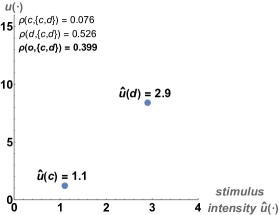
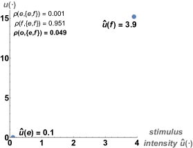
Case 1: the $\widehat{u}$-sum is constant in all menus

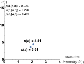
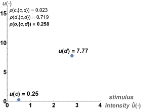
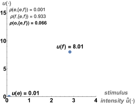
Case 2: the $u$-sum is constant in all menus

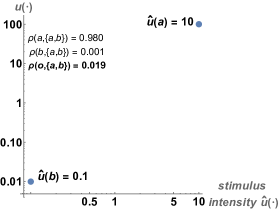
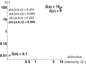
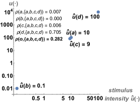
(b) “Roller-coaster” choice-overload effect (log-scaled graph)

Figure C2: Four empirically supported predictions of the reciprocal-differences model (all graphs are to scale; utilities are symmetric Cobb-Douglas and $\lambda=8$; the last example assumes additivity of $D$)

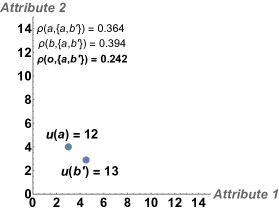
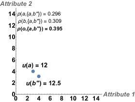
(a) Similarity-driven deferral effect

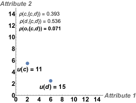
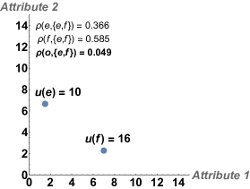
(b) Relative-attractiveness effect

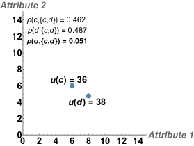
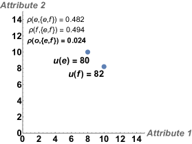
(c) Absolute-attractiveness effect

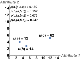
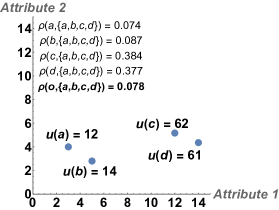
(d) “Roller-coaster” choice-overload effect

Online Supplementary Appendix

Appendix A Monotonic Decision-Conflict Logit

This class of models, introduced in Section 2, is characterized by the following condition on choice probabilties:

AA1 (Active-Choice Lower Bounds)
For all $A,B\in{\mathcal{M}}$ such that $A\supset B$:

$$\rho(B,B) \geq \frac{\displaystyle\frac{\rho(o,B)-\rho(o,A)}{\rho(o,A)}}{\displaystyle\frac{\rho(A,A)-\rho(B,A)}{\rho(B,A)}}$$

The numerator on the right hand side of this inequality is the percentage change in the probability of opting out when the agent moves from the larger menu $A$ to the smgaller menu $B$. The denominator on the other hand is the percentage increase in the probability of making an active choice at menu $A\supset B$ that is contributed by those alternatives that are available in $A$ but not in $B$. When $\rho(o,B)\geq\rho(o,A)$ holds, then AA1 and $\rho(B,B)\in(0,1)$ together imply that the percentage decrease in the probability of deferring when moving from $B$ to $A$ is strictly lower –and in proportion to $\rho(B,B)$– than the percentage increase in the probability of making an active choice at $A$ when moving from the submenu $B$ to all of $A$. When $\rho(o,A)\geq\rho(o,B)$ holds instead, then AA1 is trivially satisfied. Thus, the axiom can be thought of as allowing for deferral to become less likely in larger menus while at the same time imposing an upper bound on how less likely it can become.

Proposition 5

A decision-conflict logit is monotonic iff it satisfies AA1.

Conditional on this result, it is also immediate that strictly monotonic models are characterized by the special case of AA1 where the inequality is always strict.

Proof of Proposition 5.

Let $\rho=(u,D)$ be a decision-conflict logit and suppose $A\supset B$. By (3) and (4), $D$ is monotonic iff

$$D(A)\geq D(B) \Longleftrightarrow \frac{\rho(o,A)}{1-\rho(o,A)}\frac{\rho(A,X)}{\rho(z,X)}\geq\frac{\rho(o,B)}{1-\rho(o,B)}\frac{\rho(B,X)}{\rho(z,X)}$$

$$\Longleftrightarrow \rho(o,A)\frac{\rho(A,X)}{\rho(A,A)}\geq\rho(o,B)\frac{\rho(B,X)}{\rho(B,B)}$$

$$\Longleftrightarrow \rho(o,A)\frac{\rho(A,X)}{\rho(B,X)}\geq\rho(o,B)\frac{\rho(A,A)}{\rho(B,B)}$$

$$\Longleftrightarrow \rho(o,A)\left(\frac{\rho(B,X)+\rho(A\setminus B,X)}{\rho(B,X)}\right)\geq\rho(o,B)\frac{\rho(A,A)}{\rho(B,B)}$$

$$\Longleftrightarrow 1+\frac{\rho(A\setminus B,X)}{\rho(B,X)}\geq\frac{\rho(o,B)}{\rho(o,A)}\frac{\rho(A,A)}{\rho(B,B)}$$

$$\Longleftrightarrow \frac{\rho(A\setminus B,X)}{\rho(B,X)}\geq\frac{\rho(o,B)\rho(A,A))}{\rho(o,A)(\rho(B,B)}-\frac{\rho(o,A)\rho(B,B)}{\rho(o,A)\rho(B,B)}$$

$$\Longleftrightarrow \frac{\rho(A\setminus B,X)}{\rho(B,X)}\geq\frac{\rho(o,B)-\rho(o,A)}{\rho(o,A)\rho(B,B)}$$

$$\Longleftrightarrow \frac{\rho(A\setminus B,A)}{\rho(B,A)}\geq\frac{\rho(o,B)-\rho(o,A)}{\rho(o,A)\rho(B,B)},$$

where the last step follows from A2 and the last inequality is equivalent to AA1. $\blacksquare$

Appendix B General Utility-Difference Models

To generalize the reciprocal utility differences model we start by defining a decision-conflict logit $\rho=(u,D)$ as having a utility-difference representation if there is a strictly decreasing function $f:\mathbb{R}\rightarrow\mathbb{R}$ such that, for all $a,b\in X$,

$$D(\{a,b\}) = f\big{(}|u(a)-u(b)|\bigr{)}.$$ (47)

This model is characterized by the following axiom:

AA2 (Odds-Ratio Boundedness).
For all $a,b,c,d\in X$ such that $\rho(a,\{a,b\})>\rho(b,\{a,b\})$ and $\rho(c,\{c,d\})>\rho(d,\{c,d\})$:

$$\rho(a,\{a,b\})-\rho(b,\{a,b\})\geq\rho(c,\{c,d\})-\rho(d,\{c,d\}) \Longleftrightarrow \frac{\displaystyle\frac{\rho(o,\{a,b\})}{\rho(a,\{a,b\})}}{\displaystyle\frac{\rho(o,\{c,d\})}{\rho(c,\{c,d\})}}\leq\frac{\rho(c,\{a,c\})}{\rho(a,\{a,c\})}$$

AA2 dictates that $a$ is more likely to be chosen over $b$ than $c$ is to be chosen over $d$ in the respective binary menus iff the odds ratio of deferring relative to choosing the more probable options $a$ and $c$ is bounded above by the odds of choosing $c$ vs $a$ at the respective menu. An interesting implication of this condition is uncovered when the deferral odds ratio in question is greater than one. This implies that deferring is itself more likely at $\{a,b\}$ than it is at $\{c,d\}$. In this case A6 requires that $c$ be more choice-probable than $a$ at $\{a,c\}$, and in no smaller proportion than that associated with the deferral odds ratio. Intuitively, when opting out is less likely at $\{c,d\}$ despite the fact that $c$, $d$ are closer in probability than $a$, $b$ are at $\{a,b\}$, one might attribute this to $c$, $d$ being more valuable than $a$, $b$. Such greater value at $\{c,d\}$ may in turn have an offsetting active-choice effect at $\{c,d\}$ and also translate into $c$ being more choice-probable than $a$ at $\{a,c\}$. We come back to this point when discussing the “absolute attractiveness” effect later in this section.

Proposition 6

A decision-conflict logit $\rho=(u,D)$ is a utility-difference model iff it satisfies AA2.

Proof of Proposition 6.

Suppose $\rho=(u,D)$ satisfies AA2. To prove the claim that there exists a strictly decreasing $f:\mathbb{R}\rightarrow\mathbb{R}$ with the required property it suffices to show that, for any $a,b,c,d\in X$, $D(\{a,b\})\geq D(\{c,d\})$ $\Leftrightarrow$ $|u(a)-u(b)|\leq|u(c)-u(d)|$. To this end, consider $a,b,c,d\in X$ and assume, without loss of generality, that $\rho(a,\{a,b\})\geq\rho(b,\{a,b\})$ and $\rho(c,\{c,d\})\geq\rho(d,\{c,d\})$. By (3), this is equivalent to $u(a)\geq u(b)$ and $u(c)\geq u(d)$. Let $\alpha-\beta:=\rho(a,\{a,b\})-\rho(b,\{a,b\})$ and $\gamma-\delta:=\rho(c,\{c,d\})-\rho(d,\{c,d\})$. The above, together with A2 and AA2, implies

$$u(a)-u(b)\geq u(c)-u(d) \Longleftrightarrow \alpha-\beta\geq\gamma-\delta$$

$$\Longleftrightarrow \frac{\displaystyle\frac{\rho(o,\{a,b\})}{\rho(a,\{a,b\})}}{\displaystyle\frac{\rho(o,\{c,d\})}{\rho(c,\{c,d\})}}\leq\frac{\rho(c,\{a,c\})}{\rho(a,\{a,c\})}$$

$$\Longleftrightarrow \frac{\displaystyle\frac{\rho(o,\{a,b\})}{\rho(a,\{a,b\})}}{\displaystyle\frac{\rho(o,\{c,d\})}{\rho(c,\{c,d\})}}\leq\displaystyle\frac{\rho(c,X)}{\rho(a,X)}$$

$$\Longleftrightarrow \frac{\rho(o,\{a,b\})\rho(a,X)}{\rho(a,\{a,b\})\rho(z,X)}\leq\frac{\rho(o,\{c,d\})\rho(c,X)}{\rho(c,\{c,d\})\rho(z,X)}$$

$$\Longleftrightarrow \frac{\rho(o,\{a,b\})}{1-\rho(o,\{a,b\})}\frac{\rho(\{a,b\},X)}{\rho(z,X)}\leq\frac{\rho(o,\{c,d\})}{1-\rho(o,\{c,d\})}\frac{\rho(\{c,d\},X)}{\rho(z,X)}$$

$$\Longleftrightarrow D(\{a,b\})\leq D(\{c,d\}),$$

where, as in (3), $z\in X$ is arbitrary and such that, for some $\alpha>0$, $u(f):=\alpha\frac{\rho(f,X)}{\rho(z,X)}$. $\blacksquare$

References

- Alós-Ferrer et al. (2021) Alós-Ferrer, C., E. Fehr, and N. Netzer (2021): “Time Will Tell: Recovering Preferences When Choices Are Noisy,” Journal of Political Economy, 129, 1828–1877.
- Anderson et al. (1992) Anderson, S. P., A. de Palma, and J.-F. Thisse (1992): Discrete Choice Theory of Product Differentiation, Cambridge, MA: MIT Press.
- Apesteguia et al. (2017) Apesteguia, J., M. A. Ballester, and J. Lu (2017): “Single-Crossing Random Utility Models,” Econometrica, 85, 661–674.
- Bachi and Spiegler (2018) Bachi, B. and R. Spiegler (2018): “Buridanic Competition,” Games and Economic Behavior, 107, 298–315.
- Baldassi et al. (2020) Baldassi, C., S. Cerreia-Vioglio, F. Maccheroni, M. Marinacci, and M. Pirazzini (2020): “A Behavioral Characterization of the Drift Diffusion Model and its Multi-alternative Extension for Choice under Time Pressure,” Management Science, 66, 5075–5093.
- Baldassi et al. (2021) ——— (2021): “Multialternative Neural Decision Processes,” Working Paper.
- Bhatia and Mullett (2016) Bhatia, S. and T. L. Mullett (2016): “The Dynamics of Deferred Decision,” Cognitive Psychology, 86, 112–151.
- Bhatia and Mullett (2018) ——— (2018): “Similarity and Decision Time in Preferential Choice,” Quarterly Journal of Experimental Psychology, 71, 1276–1280.
- Block and Marschak (1960) Block, H. D. and J. Marschak (1960): “Random Orderings and Stochastic Theories of Response,” in Contributions to Probability and Statistics: Essays in Honor of Harold Hotelling, ed. by I. Olkin, Stanford, CA: Stanford University Press, 97–132.
- Bordallo et al. (2013) Bordallo, P., N. Gennaioli, and A. Shleifer (2013): “Salience and Consumer Choice,” Journal of Political Economy, 121, 803–843.
- Buturak and Evren (2017) Buturak, G. and O. Evren (2017): “Choice Overload and Asymmetric Regret,” Theoretical Economics, 12, 1029–1056.
- Carroll et al. (2009) Carroll, G. D., J. J. Choi, D. Laibson, B. C. Madrian, and A. Metrick (2009): “Optimal Defaults and Active Decisions,” Quarterly Journal of Economics, 124, 1639–1674.
- Chernev et al. (2015) Chernev, A., U. Böckenholt, and J. Goodman (2015): “Choice Overload: A Conceptual Review and Meta-Analysis,” Journal of Consumer Psychology, 25, 333–358.
- Costa-Gomes et al. (2022) Costa-Gomes, M., C. Cueva, G. Gerasimou, and M. Tejiščák (2022): “Choice, Deferral and Consistency,” Quantitative Economics, 13, 1297–1318.
- Dhar (1997) Dhar, R. (1997): “Consumer Preference for a No-Choice Option,” Journal of Consumer Research, 24, 215–231.
- Dhar and Simonson (2003) Dhar, R. and I. Simonson (2003): “The Effect of Forced Choice on Choice,” Journal of Marketing Research, 40, 146–160.
- Echenique et al. (2018) Echenique, F., K. Saito, and G. Tserenjigmid (2018): “The Perception-Adjusted Luce Model,” Mathematical Social Sciences, 93, 67–76.
- Falmagne (2002) Falmagne, J. C. (2002): Elements of Psychophysical Theory, Oxford: Oxford University Press.
- Frick (2016) Frick, M. (2016): “Monotone Threshold Representations,” Theoretical Economics, 11, 757–772.
- Fudenberg et al. (2015) Fudenberg, D., R. Iijima, and T. Strzalecki (2015): “Stochastic Choice and Revealed Perturbed Utility,” Econometrica, 83, 2371–2409.
- Gerasimou (2018) Gerasimou, G. (2018): “Indecisiveness, Undesirability and Overload Revealed Through Rational Choice Deferral,” Economic Journal, 128, 2450–2479.
- Gerasimou and Papi (2018) Gerasimou, G. and M. Papi (2018): “Duopolistic Competition with Choice-Overloaded Consumers,” European Economic Review, 101, 330–353.
- Hensher et al. (2015) Hensher, D. A., J. M. Rose, and W. H. Greene (2015): Applied Choice Analysis, New York: Cambridge University Press.
- Horan (2019) Horan, S. (2019): “Random Consideration and Choice: A Case Study of Default Options,” Mathematical Social Sciences, 102, 73–84.
- Iyengar and Kamenica (2010) Iyengar, S. S. and E. Kamenica (2010): “Choice Proliferation, Simplicity Seeking, and Asset Allocation,” Journal of Public Economics, 94, 530–539.
- Iyengar and Lepper (2000) Iyengar, S. S. and M. R. Lepper (2000): “When Choice is Demotivating: Can One Desire Too Much of a Good Thing?” Journal of Personality and Social Psychology, 79, 995–1006.
- Knops et al. (2013) Knops, A. M., D. T. Ubbink, D. A. Legemate, L. J. Stalpers, and P. M. Bossuyt (2013): “Interpreting Patient Decisional Conflict Scores: Behavior and Emotions in Decisions about Treatment,” Medical Decision Making, 33, 78–84.
- Kovach and Tserenjigmid (2022a) Kovach, M. and G. Tserenjigmid (2022a): “Behavioral Foundations of Nested Stochastic Choice and Nested Logit,” Journal of Political Economy, 130, 2411–2462.
- Kovach and Tserenjigmid (2022b) ——— (2022b): “The Focal Luce Model,” American Economic Journal: Microeconomics, 14, 378–413.
- Krajbich et al. (2010) Krajbich, I., C. Armel, and A. Rangel (2010): “Visual Fixations and the Computation and Comparison of Value in Simple Choice,” Nature Neuroscience, 13, 1292–1298.
- Luce (1959) Luce, R. D. (1959): Individual Choice Behavior: A Theoretical Analysis, New York, NY: Wiley.
- Luce and Suppes (1965) Luce, R. D. and P. Suppes (1965): “Preference, Utility and Subjective Probability,” in Handbook of Mathematical Psychology, Volume 3, ed. by R. D. Luce, R. R. Bush, and E. H. Galanter, New York: Wiley, 249–410.
- Manzini and Mariotti (2014) Manzini, P. and M. Mariotti (2014): “Stochastic Choice and Consideration Sets,” Econometrica, 83, 1153–1176.
- McFadden (1973) McFadden, D. (1973): “Conditional Logit Analysis of Qualitative Choice Behavior,” in Frontiers in Econometrics, ed. by P. Zarembka, New York: Academic Press, 105–142.
- Milosavljevic et al. (2010) Milosavljevic, M., J. Malmaud, A. Huth, C. Koch, and A. Rangel (2010): “The Drift Diffusion Model Can Account for the Accuracy and Reaction Time of Value-Based Choices under High and Low Time Pressure,” Judgment and Decision Making, 5, 437–449.