Boosting Ant Colony Optimization via Solution Prediction
and Machine Learning

Abstract

This paper introduces an enhanced meta-heuristic (ML-ACO) that combines machine learning (ML) and ant colony optimization (ACO) to solve combinatorial optimization problems. To illustrate the underlying mechanism of our ML-ACO algorithm, we start by describing a test problem, the orienteering problem. In this problem, the objective is to find a route that visits a subset of vertices in a graph within a time budget to maximize the collected score. In the first phase of our ML-ACO algorithm, an ML model is trained using a set of small problem instances where the optimal solution is known. Specifically, classification models are used to classify an edge as being part of the optimal route, or not, using problem-specific features and statistical measures. The trained model is then used to predict the ‘probability’ that an edge in the graph of a test problem instance belongs to the corresponding optimal route. In the second phase, we incorporate the predicted probabilities into the ACO component of our algorithm, i.e., using the probability values as heuristic weights or to warm start the pheromone matrix. Here, the probability values bias sampling towards favoring those predicted ‘high-quality’ edges when constructing feasible routes. We have tested multiple classification models including graph neural networks, logistic regression and support vector machines, and the experimental results show that our solution prediction approach consistently boosts the performance of ACO. Further, we empirically show that our ML model trained on small synthetic instances generalizes well to large synthetic and real-world instances. Our approach integrating ML with a meta-heuristic is generic and can be applied to a wide range of optimization problems.

1 Introduction

Ant colony optimization (ACO) is a class of widely-used meta-heuristics, inspired by the foraging behavior of biological ants, for solving combinatorial optimization problems [Dorigo et al., 1996, Dorigo & Gambardella, 1997]. Since its introduction in early 1990s, ACO has been extensively investigated to understand both its theoretical foundations and practical performance [Dorigo & Blum, 2005, Blum, 2005]. A lot of effort has been made to improve the performance of ACO, making it one of the most competitive algorithms for solving a wide range of optimization problems. Whilst ACO cannot provide any optimality guarantee due to its heuristic nature, it is usually able to find a high-quality solution for a given problem within a limited computational budget.

The ACO algorithm builds a probabilistic model to sample solutions for an optimization problem. In this sense, ACO is closely related to Estimation of Distribution Algorithms and Cross Entropy methods [Zlochin et al., 2004]. The probabilistic model of ACO is parametrized by a so-called pheromone matrix and a heuristic weight matrix, which basically measure the ‘payoff’ of setting a decision variable to a particular value. The aim of ACO is to evolve the pheromone matrix so that an optimal (or a near-optimal) solution can be generated via the probabilistic model in sampling. Previously, the pheromone matrix is usually initialized uniformly and the heuristic weights are set based on prior domain knowledge. In this paper, we develop machine learning (ML) techniques to warm start the pheromone matrix or identify good heuristic weights for ACO to use.

Leveraging ML to help combinatorial optimization has attracted much attention recently [Bengio et al., 2021, Karimi-Mamaghan et al., 2022]. For instance, novel ML techniques have been developed to prune the search space of large-scale optimization problems to a smaller size that is manageable by existing solution algorithms [Sun et al., 2021b, Lauri & Dutta, 2019, Sun et al., 2021a], to order decision variables for branch and bound or tree search algorithm [Li et al., 2018b, Shen et al., 2021], and to approximate the objective value of solutions [Fischetti & Fraccaro, 2019, Santini et al., 2021]. There also exist ML-based methods that try to directly predict a high-quality solution for an optimization problem [Abbasi et al., 2020, Ding et al., 2020]. The key idea of these methods is typically solution prediction via ML; that is aiming to predict the optimal solution for a given problem as close as possible.

Building upon these previous studies, we propose an enhanced meta-heuristic named ML-ACO, that combines ML (more specifically solution prediction) and ACO to solve combinatorial optimization problems. To illustrate the underlying mechanism of our proposed algorithm, we first describe the orienteering problem, which is also used to demonstrate the efficacy of ML-ACO. The aim of orienteering problem is to search for a route in a graph that visits a subset of vertices within a given time budget to maximize the total score collected from the visited vertices (see Section 2.1 for a formal definition). The orienteering problem has many real-world applications [Vansteenwegen et al., 2011, Gunawan et al., 2016].

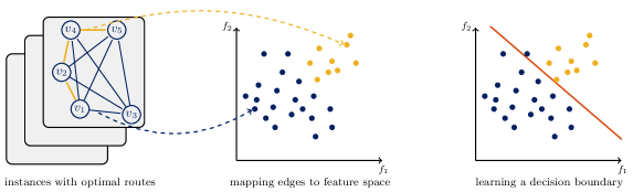
Figure 1: An illustration of the training procedure of our ML model. First, a set of orienteering problem instances are solved, with the optimal route highlighted in yellow in the corresponding graph of orienteering problem instance (left figure). We then extract features (e.g., edge weight) to describe each edge of the graphs, and map each edge to the feature space as a training point (middle figure). Finally, we apply a classification algorithm to learn a decision boundary in the feature space to well separate edges (training points) that are part of the optimal routes from those which are not (right figure).

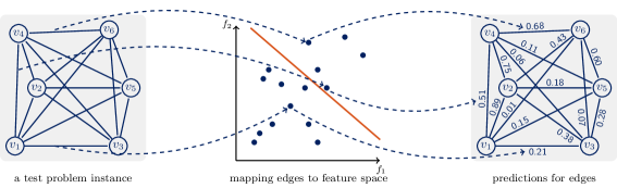
Figure 2: The testing procedure of our ML model. Given an unsolved test orienteering problem instance (left figure), we first map each edge of the corresponding graph to a point in the feature space (middle figure). Based on the location of the points with respect to the decision boundary learned in training, we can compute for each edge a probability that it belongs to an optimal route (right figure). The predictions are then used to bias the sampling of ACO towards using the edges with a larger predicted probability value more often when constructing feasible routes.

In the first phase of our ML-ACO algorithm, an ML model is trained on a set of optimally-solved small orienteering problem instances with known optimal route, as shown in Figure 1. We extract problem-specific features as well as statistical measures (see Section 3.1) to describe each edge in the graphs of solved orienteering problem instances, and map each edge to a training point in the feature space. Classification algorithms can then be used to learn a decision boundary in the feature space to differentiate the edges that are in the optimal routes from those which are not. We have tested multiple existing classification algorithms for this task including graph neural networks [Kipf & Welling, 2017, Wu et al., 2021], logistic regression [Bishop, 2006] and support vector machines [Boser et al., 1992, Cortes & Vapnik, 1995]. For an unsolved test orienteering problem instance, the trained ML model can then be used to predict the ‘probability’ that an edge in the corresponding graph belongs to the optimal route, as shown in Figure 2.

In the second phase of our ML-ACO algorithm, we incorporate the probability values predicted by our ML model into the ACO algorithm, i.e., using the probability values to set the heuristic weight matrix or to initialize the pheromone matrix of ACO. The aim is to bias the sampling of ACO towards favoring the edges that are predicted more likely to be part of an optimal route, and hopefully to improve the efficiency of ACO in finding high-quality routes. In this sense, the idea of our ML-ACO algorithm is also related to the seeding strategies that are used to improve evolutionary algorithms [Liaw, 2000, Hopper & Turton, 2001, Friedrich & Wagner, 2015, Chen et al., 2018].

We use simulation experiments to show the efficacy of our ML-ACO algorithm on the orienteering problem. The results show that our ML-ACO algorithm significantly improves over the classic ACO in finding high-quality solutions. We also test the use of different classification algorithms, and observe that our solution prediction approach consistently boosts the performance of ACO. Finally, we show that our ML model trained on small synthetic problem instances generalizes well to large synthetic instances as well as real-world instances.

In summary, we have made the following contributions:

• This paper is the first attempt, to our knowledge, at boosting the performance of the ACO algorithm via solution prediction and ML.

• We empirically show that our proposed ML-ACO algorithm significantly improves over the classic ACO, no matter which classification algorithm is used in training.

• We also demonstrate the generalization capability of ML-ACO on large synthetic and real-world problem instances.

The remainder of this paper is organized as follows. In Section 2, we introduce the orienteering problem and the ACO algorithm. In Section 3, we describe the proposed ML-ACO algorithm. Section 4 presents our experimental results, and the last section concludes the paper and shows potential avenues for future research.

2 Background and Related Work

We first describe the orienteering problem and then introduce the ACO algorithm in the context of orienteering problem.

2.1 Orienteering problem

The orienteering problem finds its application in many real-world problems, such as tourist trip planning, home fuel delivery and building telecommunication networks [Vansteenwegen et al., 2011, Gunawan et al., 2016]. Consider a complete undirected graph $G(V,E,S,C)$, where $V=\{v_{1},\ldots,v_{n}\}$ denotes the vertex set, $E=\{e_{i,j}\,|\,1\leq i\neq j\leq n\}$ denotes the edge set, $S=\{s_{1},\ldots,s_{n}\}$ denotes the score of each vertex, and $C=\{c_{i,j}\,|\,1\leq i\neq j\leq n\}$ denotes the time cost of traveling through each edge. Assume $v_{1}$ is the starting vertex and $v_{n}$ is the ending vertex. The objective of the orienteering problem is to search for a path from $v_{1}$ to $v_{n}$ that visits a subset of vertices within a given time budget $T_{\mathrm{max}}$, such that the total score collected is maximized. Thus, the orienteering problem can be viewed as a combination of traveling salesman problem and knapsack problem. We use $u_{i}$ to denote the visiting order of vertex $v_{i}$, and use a binary variable $x_{i,j}$ to denote whether vertex $v_{j}$ is visited directly after vertex $v_{i}$. The integer program of the orienteering problem can be written as:

$$\max_{\bm{x},\bm{u}} \sum_{i=1}^{n-1}\sum_{j=2}^{n}s_{j}x_{i,j},$$ (1)

$$s.t.\;\, \sum_{j=1}^{n}x_{1,j}=\sum_{i=1}^{n}x_{i,n}=1,$$ (2)

$$\sum_{i=1}^{n-1}x_{i,k}=\sum_{j=2}^{n}x_{k,j}\leq 1,\; 2\leq k\leq n-1;$$ (3)

$$u_{i}-u_{j}+1\leq(n-1)(1-x_{i,j}), 2\leq i,j\leq n;$$ (4)

$$\sum_{i=1}^{n-1}\sum_{j=2}^{n}c_{i,j}x_{i,j}\leq T_{\mathrm{max}},$$ (5)

$$u_{i}\geq 0,\; 2\leq i\leq n;$$ (6)

$$x_{i,j}\in\{0,1\},\; 1\leq i,j\leq n.$$ (7)

The constraints (2) ensure that the path starts from vertex $1$ and ends in vertex $n$. The constraints (3) guarantee that each vertex in between can only be visited at most once. The constraints (4) are the Miller-Tucker-Zemlin subtour elimination constraints, and the constraint (5) satisfies the given time budget. Note that this formulation is not computationally efficient, and there are some relatively trivial ways to make it slightly stronger [Fischetti et al., 1998]. However, this formulation is sufficient for logical correctness.

The orienteering problem is NP-hard [Golden et al., 1987]. Many solution methods have been proposed to solve the orienteering problem and its variants, including exact solvers [Fischetti et al., 1998, El-Hajj et al., 2016, Archetti et al., 2016, Angelelli et al., 2017] and heuristics or meta-heuristics [Kobeaga et al., 2018, Santini, 2019, Hammami et al., 2020, Assunção & Mateus, 2021]. Solving the orienteering problem to optimality using exact solvers may take a long time, especially for large instances. However, in some real-world applications such as tourist trip planning, we need to provide a high-quality solution to users within a short time. In this case, meta-heuristics are useful to search for a high-quality solution when the computational budget is very limited. In the next subsection, we describe the meta-heuristic, ACO, to solve the orienteering problem.

2.2 Ant colony optimization

The ACO algorithm is inspired by the behavior of biological ants seeking the shortest path between food and their colony [Dorigo et al., 1996, Dorigo & Gambardella, 1997]. Unlike many other nature inspired algorithms, ACO has a solid mathematical foundation, based on probability theory. The underlying mechanism of ACO is to build a parametrized probabilistic model to incrementally construct feasible solutions. The parameters of this probabilistic model are evolved over time, based on the sample solutions generated in each iteration of the algorithm. By doing this, better solution components are reinforced, leading to an optimal (or near-optimal) solution in the end. The ACO algorithm has been demonstrated to be effective in solving various combinatorial optimization problems [Dorigo & Blum, 2005, Blum, 2005, Mavrovouniotis et al., 2016, Xiang et al., 2021, Jia et al., 2021, Palma-Heredia et al., 2021].

As our main focus is to investigate whether ML can be used to improve the performance of ACO, we simply test on two representative ACO models – Ant System (AS) [Dorigo et al., 1996] and Max-Min Ant System (MMAS) [Stützle & Hoos, 2000]. The AS is one of the original ACO algorithms, and MMAS is a well-performing variant [Blum, 2005]. Note that ACO has been applied to solve the orienteering problem variants, e.g., team orienteering problem [Ke et al., 2008], team orienteering problem with time windows [Montemanni et al., 2011, Gambardella et al., 2012] and time-dependent orienteering problem with time windows [Verbeeck et al., 2014, 2017]. These works are typically based on one of the early ACO models, possibly integrated with local search methods. To avoid complication, we simply select the AS and MMAS models, which are sufficient for our study.

The AS algorithm uses a population of $m$ ants to incrementally construct feasible solutions based on a parametrized probabilistic model. For the orienteering problem, a feasible solution is a path, consisting of a set of connected edges. In one iteration of the algorithm, each of the $m$ ants constructs its own path from scratch. Starting from $v_{1}$, an ant incrementally selects the next vertex to visit until all the time budget is used up. Note that as $v_{n}$ is the ending vertex, each ant should reserve enough time to visit $v_{n}$.

Suppose an ant is at vertex $v_{i}$, and $V_{i}$ denotes the set of vertices that this ant can visit in the next step without violating the time budget constraint. The probability of this ant visiting vertex $v_{j}\in V_{i}$ in the next step is defined by

$$p_{i,j}=\frac{\tau_{i,j}^{\alpha}\eta_{i,j}^{\beta}}{\sum\limits_{k\in V_{i}}\tau_{i,k}^{\alpha}\eta_{i,k}^{\beta}},$$ (8)

where $\tau_{i,j}$ is the amount of pheromone deposited by the ants for transition from vertex $v_{i}$ to $v_{j}$; $\eta_{i,j}$ is the desirability of transition from vertex $v_{i}$ to $v_{j}$; $\alpha\geq 0$ and $\beta\geq 0$ are control parameters. This means the probability of visiting vertex $v_{j}\in V_{i}$ from $v_{i}$ is proportional to the product of $\tau_{i,j}^{\alpha}\eta_{i,j}^{\beta}$.

The desirability of transition from vertex $v_{i}$ to $v_{j}$, i.e., $\eta_{i,j}$, is usually set based on prior knowledge. In the orienteering problem, we can set $\eta_{i,j}$ to the ratio of the score collected at vertex $v_{j}$ to the time required for travelling from vertex $v_{i}$ to $v_{j}$: $\eta_{i,j}=s_{j}/c_{i,j}$. This computes the score that can be collected per unit time if travelling through edge $e_{i,j}$, and measures the ‘payoff’ of including edge $e_{i,j}$ in the path in terms of the objective value. By using these $\bm{\eta}$ values, high-quality edges (i.e., those allowing for a large collected score per unit time) are more likely to be sampled.

The pheromone values $\bm{\tau}$ are typically initialized uniformly, and are gradually evolved in each iteration of the algorithm, such that the components (edges) of high-quality sample solutions gradually acquire a large pheromone value. This also biases the sampling to using high-quality edges more often. In each iteration, after all the $m$ ants have completed their solution construction process, the pheromone values $\tau_{i,j}$, where $i,j=1,\ldots,n$ and $i\neq j$, are updated based on the sample solutions generated:

$$\tau_{i,j}=(1-\rho)\tau_{i,j}+\sum_{k=1}^{m}\Delta\tau_{i,j}^{k},$$ (9)

where $\rho>0$ is the pheromone evaporation coefficient, and $\Delta\tau_{i,j}^{k}$ is the amount of pheromone deposited by the $k^{\mathrm{th}}$ ant on edge $e_{i,j}$. Let $y_{k}$ denote the objective value collected by the $k^{\mathrm{th}}$ ant, and $C>0$ be a constant. We can define $\Delta\tau_{i,j}^{k}=y_{k}/C$, if edge $e_{i,j}$ is used by the $k^{\mathrm{th}}$ ant; otherwise $\Delta\tau_{i,j}^{k}=0$. The amount of pheromone deposited by an ant when it travels along a path is proportional to the objective value of the path. As we are solving a maximization problem, edges that appear in high-quality paths are reinforced (i.e., acquiring a large pheromone value), so that these edges are more likely to be used when constructing paths in the later iterations. This sampling and evolving process is repeated for a predetermined number of iterations, and the best solution generated is returned in the end.

The MMAS algorithm is a variant of AS, which uses the same probabilistic model (Eq. 8) to construct feasible solutions. The key difference between MMAS and AS is how the pheromone matrix ($\bm{\tau}$) is updated. The MMAS algorithm only uses a single solution to update the pheromone matrix in each iteration, in contrast to AS which uses a population of $m$ solutions. This single solution can either be the best solution generated in the current iteration (iteration-best) or the best one found so far (global-best). The use of a single best solution makes the search more greedy towards high-quality solutions, in the sense that only the edges in the best solution get reinforced. Let $\bm{x}^{\mathrm{best}}$ denote the best solution and $y^{\mathrm{best}}$ be the objective value of $\bm{x}^{\mathrm{best}}$. The pheromone values $\tau_{i,j}$ for each pair of $i,j=1,\ldots,n$ and $i\neq j$ are updated as

$$\tau_{i,j}=(1-\rho)\tau_{i,j}+\Delta\tau_{i,j}^{\mathrm{best}},$$ (10)

where $\Delta\tau_{i,j}^{\mathrm{best}}=1/y^{\mathrm{best}}$ if edge $e_{i,j}$ is in the best solution $\bm{x}^{\mathrm{best}}$; otherwise $\Delta\tau_{i,j}^{\mathrm{best}}=0$.

The second key difference between MMAS and AS is that the pheromone values in MMAS are restricted to a range of $[\tau_{\mathrm{min}},\tau_{\mathrm{max}}]$. After the pheromone values have been updated in each iteration using Eq. (10), if a pheromone value $\tau_{i,j}>\tau_{\mathrm{max}}$, we reset it to the upper bound $\tau_{\mathrm{max}}$. This avoids the situation where an edge accumulates a very large pheromone value, such that it is (almost) always selected in sampling based on the probabilistic model. The upper bound on pheromone values is derived as

$$\tau_{\mathrm{max}}=\frac{1}{\rho\cdot y^{\mathrm{opt}}},$$ (11)

where $y^{\mathrm{opt}}$ is the optimal solution of the problem instance. In practice, we often substitute $y^{\mathrm{opt}}$ with the best solution found so far to compute the upper bound, since we do not have $y^{\mathrm{opt}}$ before solving the problem. Similarly if a pheromone value $\tau_{i,j}<\tau_{\mathrm{min}}$, we reset it to the lower bound $\tau_{\mathrm{min}}$. This ensures the probability of selecting any edge in sampling does not reduce to zero. In this sense, the probability of generating the optimal solution via sampling approaches one if given an infinite amount of time. We simply set the lower bound to

$$\tau_{\mathrm{min}}=\frac{\tau_{\mathrm{max}}}{2n},$$ (12)

where $n$ is the problem dimensionality. This setting is consistent with the original paper [Stützle & Hoos, 2000] for solving the traveling salesman problem.

The MMAS algorithm also uses an additional mechanism called pheromone trail smoothing to deal with premature convergence. When the algorithm has converged, the pheromone values are increased proportionally to their difference to $\tau_{\mathrm{max}}$:

$$\tau_{i,j}=\tau_{i,j}+\delta\cdot(\tau_{\mathrm{max}}-\tau_{i,j}),$$ (13)

where $0\leq\delta\leq 1$ is a control parameter. In the extreme case $\delta=1$, it is equivalent to restarting the algorithm, in the sense that the pheromone values are reinitialized uniformly to $\tau_{\mathrm{max}}$. We activate the pheromone trail smoothing mechanism if there is no improvement in the objective value for a predetermined number of consecutive iterations $T_{\mathrm{pts}}$.

3 Boosting Ant Colony Optimization via Solution Prediction

This section presents the proposed ML-ACO algorithm, that integrates ML with ACO to solve the orienteering problem. The main idea of our ML-ACO algorithm is first to develop an ML model, aiming to predict the probability that an edge in the graph of an orienteering problem instance belongs to the optimal route. The training and testing procedures of our ML model are illustrated in Figure 1 and 2 respectively. The predicted probability values are then leveraged to improve the performance of ACO in finding high-quality solutions.

In the first phase of our ML-ACO algorithm, we construct a training set from small orienteering problem instances (graphs), that are solved to optimality by a generic exact solver – CPLEX. We treat each edge in a solved graph as a training point, and extract several graph features as well as statistical measures to characterize each edge (Section 3.1). The edges that are part of the optimal route obtained by CPLEX are called positive training points and labelled as $1$; otherwise they are negative training points labelled as $-1$. Note that the decision variables of the edges that do not belong to the optimal route have a value of zero in the optimal solution produced by CPLEX. We call these edges negative training points to be consistent with the ML literature. This then becomes a binary classification problem, where the goal is to learn a decision rule based on the extracted features to well separate the positive and negative training points. We will test multiple classification algorithms for this task. Given an unsolved orienteering problem instance, the trained ML model can then be applied to predict for each edge a probability that it belongs to the optimal route (Section 3.2).

In the second phase of ML-ACO, the probability values predicted by our ML model are then incorporated into the probabilistic model of ACO to improve its performance. The idea is to use the edges that are predicted more likely to be in an optimal route more often in the sampling process of ACO. By doing this, high-quality routes can hopefully be generated more quickly. We will use the predicted probability values to either seed the pheromone matrix or set the heuristic weight matrix of ACO (Section 3.3).

The general procedure of our ML-ACO algorithm can be summarized as follows:

1. Solve small orienteering problem instances to optimality using CPLEX;

2. Construct a training set from the optimally-solved problem instances;

3. Train an ML model offline to separate positive and negative training points (edges) in our training set;

4. Predict which edges are more likely to be in an optimal route for a test (unsolved) problem instance;

5. Incorporate solution prediction into ACO to boost its performance.

Note that our ML model is based on the edge representation of solutions for the orienteering problem, i.e., each edge in the graph belongs to a route (solution) or not. A more efficient way typically used by ACO to represent a route is using a sequence of vertices. A potential avenue for future research would be to develop an ML model based on the vertex representation to predict the order in which vertices are visited in the optimal route. This will become a multiclass classification problem in contrast to the binary classification problem developed in this paper.

3.1 Constructing training set

We construct a training set from optimally-solved orienteering problem instances on complete graphs, where each edge is a training point. We assign a class label $1$ to edges that belong to the optimal route and $-1$ to those who do not. Three graph features and two statistical measures are designed to characterize each edge, which are detailed below.

Recall that the objective of orienteering problem $G(V,E,S,C)$ is to search for a path that visits a subset of vertices within a given time budget $T_{\mathrm{max}}$, to maximize the total score collected. Three factors are relevant to the objective, i.e., vertex scores $S$, edge costs $C$ and time budget $T_{\mathrm{max}}$. The first graph feature we design to describe edge $e_{i,j}$, is the ratio between edge cost $c_{i,j}$ and the time budget $T_{\mathrm{max}}$

$$f_{1}(e_{i,j})=\frac{c_{i,j}}{T_{\mathrm{max}}},$$ (14)

where $i,j=1,\ldots,n$ and $i\neq j$. Intuitively, if $c_{i,j}>T_{\mathrm{max}}$, the edge $e_{i,j}$ certainly cannot appear in any of the feasible solutions. A stronger preprocessing criterion would be to eliminate edge $e_{i,j}$ if $c_{1,i}+c_{i,j}+c_{j,n}>T_{\mathrm{max}}$, where $v_{1}$ is the starting vertex and $v_{n}$ is the ending vertex. However, this type of exact pruning mechanism is not expected to eliminate many edges from a problem instance.

Another informative feature for describing edge $e_{i,j}$ is the ratio between vertex score $s_{j}$ and edge cost $c_{i,j}$, which computes the score we can collect immediately from vertex $v_{j}$ per unit time if taking the edge $e_{i,j}$. We normalize this ratio of edge $e_{i,j}$ by the maximum ratio of the edges that originates from vertex $v_{i}$,

$$f_{2}(e_{i,j})=\frac{s_{j}/c_{i,j}}{\max\limits_{k=1,\ldots,n}s_{k}/c_{i,k}}.$$ (15)

This normalization is useful because it computes the relative payoff of selecting edge $e_{i,j}$, comparing to the alternative ways of leaving vertex $v_{i}$. Similarly, we also normalize the ratio of edge $e_{i,j}$ by the maximum ratio of the edges that ends in vertex $v_{j}$,

$$f_{3}(e_{i,j})=\frac{s_{j}/c_{i,j}}{\max\limits_{k=1\ldots,n}s_{j}/c_{k,j}}.$$ (16)

This computes the relative payoff of visiting vertex $v_{j}$ via edge $e_{i,j}$, comparing against other ways of visiting vertex $v_{j}$. These graph features are computationally very cheap, but they only capture local characteristics of an edge. Hence, we also adopt two statistical measures, originally proposed in [Sun et al., 2021b], to capture global features of an edge.

The two statistical measures rely on random samples of feasible solutions (routes). We use the method presented in Appendix A.1 to generate $m$ random feasible solutions, denoted as $\{\bm{x}^{1},\bm{x}^{2},\ldots,\bm{x}^{m}\}$, and their objective values denoted as $\{y^{1},y^{2},\ldots,y^{m}\}$. Each solution $\bm{x}$ is a binary string, where $x_{i,j}=1$ if the edge $e_{i,j}$ is in the route; otherwise $x_{i,j}=0$. The time complexity of sampling $m$ feasible solutions for an $n$-dimensional problem instance is $\mathcal{O}(mn)$, which is proved in Appendix A.1. The sample size $m$ should be larger than $n$, otherwise there will be some edges that are never sampled. We will set $m=100n$ in our experiments, unless explicitly indicated otherwise.

The first statistical measure for characterizing edge $e_{i,j}$ is computed based on the ranking of sample solutions

$$f_{r}(e_{i,j})=\sum_{k=1}^{m}\frac{x_{i,j}^{k}}{r^{k}},$$ (17)

where $r^{k}$ denotes the ranking of the $k^{\mathrm{th}}$ sample in terms of its objective value in descending order. This ranking-based measure assigns a large score to edges that frequently appear in high-quality sample solutions, in the hope that these edges may also appear in an optimal solution. We normalize the ranking-based score of each edge by the maximum score in a problem instance to alleviate the effects of different sample size $m$

$$f_{4}(e_{i,j})=\frac{f_{r}(e_{i,j})}{\max\limits_{p,q=1,\ldots,n}f_{r}(e_{p,q})}.$$ (18)

The other statistical measure employed is a correlation-based measure, that computes the Pearson correlation coefficient between each variable $x_{i,j}$ and objective values $y$ across the sample solutions:

$$f_{c}(e_{i,j})=\frac{\sum_{k=1}^{m}(x_{i,j}^{k}-\bar{x}_{i,j})(y^{k}-\bar{y})}{\sqrt{\sum_{k=1}^{m}(x_{i,j}^{k}-\bar{x}_{i,j})^{2}}\sqrt{\sum_{k=1}^{m}(y^{k}-\bar{y})^{2}}},$$ (19)

where $\bar{x}_{i,j}=\sum_{k=1}^{m}x_{i,j}^{k}/m$, and $\bar{y}=\sum_{k=1}^{m}y^{k}/m$. As the orienteering problem is a maximization problem, edges that are highly positively correlated with the objective values are likely to be in an optimal route. Similarly, we normalize the correlation-based score of each edge by the maximum correlation value in a problem instance:

$$f_{5}(e_{i,j})=\frac{f_{c}(e_{i,j})}{\max\limits_{p,q=1,\ldots,n}f_{c}(e_{p,q})}.$$ (20)

The time complexity of directly computing these two statistical measures based on the binary string representation $\bf{x}$ is $\mathcal{O}(mn^{2})$, as we need to visit every bit in each of the $m$ binary strings. To improve the time efficiency, we adopt the method proposed in [Sun et al., 2021b], which represents the sample solutions using sets instead of strings. We then are able to compute the statistical measures in $\mathcal{O}(mn+n^{2})$ time. The details of how to efficiently compute these measures are presented in Appendix A.2.

In summary, we have extracted five features ($f_{1}$, $f_{2}$, $f_{3}$, $f_{4}$, $f_{5}$) to characterize each edge (training point). For a problem instance with $n$ vertices, we can extract $n(n-1)$ training points, as there are $n(n-1)$ directed edges in the corresponding complete graph. We use multiple solved problem instances to construct our training set $\mathbb{S}=\{(\bm{f}^{i},l^{i})\,|\,i=1,\ldots,n_{t}\}$, where $\bm{f}^{i}$ is the $5$-dimensional feature vector; $l^{i}\in\{-1,1\}$ is the class label of the $i^{\mathrm{th}}$ training point; and $n_{t}$ is the number of training points.

3.2 Training and solution prediction

After we have obtained a training set $\mathbb{S}$, our goal is then to learn a decision boundary to separate positive (label $1$) and negative (label $-1$) training points in $\mathbb{S}$ as well as possible. This is a typical binary classification problem, that can be solved by any off-the-shelf classification algorithm. To see the effects of using different classification algorithms, we compare three alternatives for this task, namely, support vector machine (SVM) [Boser et al., 1992, Cortes & Vapnik, 1995], logistic regression (LR) [Bishop, 2006], and graph convolutional network (GCN) [Kipf & Welling, 2017, Wu et al., 2021]. SVM and LR are well-known traditional algorithms with a solid mathematical foundation, and GCN is a popular deep neural network based on graph structure of a problem. This comparison is interesting, because it sheds light on whether a ‘deep’ model outperforms a ‘shallow’ model in the context of solution prediction for combinatorial optimization. A brief description of the three learning algorithms can be found in Appendix A.3.

In our training set, the number of positive training points is much smaller than that of negative training points. Considering an orienteering problem instance with $n$ vertices, the number of edges appearing in an optimal route is less than $n$, and the total number of edges in the directed complete graph is $n(n-1)$. Hence, the ratio between positive and negative edges is less than $1/(n-2)$. In this sense, our training set is highly imbalanced, and classification algorithms tend to classify negative training points better than the positive points. To address this issue, we penalize misclassifying positive training points more by using a larger regularization parameter $r^{+}$, in contrast to that of negative training points $r^{-}$ (see the loss functions (25), (28) and (30) of the classification algorithms in Appendix A.3). In our experiments, we set $r^{-}=1$ and $r^{+}=n_{-1}/n_{1}$, where $n_{-1}$ and $n_{1}$ are the number of negative and positive points in our training set.

In the testing phase, we can apply the trained model to predict a scalar $z_{i,j}$ for each edge $e_{i,j}$ in an unseen orienteering problem instance, where $i,j=1,\ldots,n$ and $i\neq j$. For GCN, $z_{i,j}$ is the output of the last layer. For SVM and LR, $z_{i,j}$ is computed as $z_{i,j}=\bm{w}_{*}^{T}\bm{f}^{i,j}+b_{*}$, where ($\bm{w}_{*}$, $b_{*}$) are the optimized parameters, and $\bm{f}^{i,j}$ is the feature vector of edge $e_{i,j}$. We then feed the predicted value $z_{i,j}$ into the logistic function to normalize it to a range of $[0,1]$:

$$p_{i,j}=\frac{1}{1+e^{-z_{i,j}}}.$$ (21)

The value of $p_{i,j}$ approaches 1 if $z_{i,j}$ approaches infinity; and $p_{i,j}$ approaches 0 when $z_{i,j}$ approaches negative infinity. In this sense, $p_{i,j}$ can be interpreted as the probability of edge $e_{i,j}$ belonging to an optimal solution. In the next subsection, we will explore multiple ways of incorporating the predicted probability values $p_{i,j}$ into ACO to guide its sampling process.

3.3 Incorporating solution prediction into ACO

Recall that the probabilistic model of ACO heavily depends on the heuristic weight matrix $\bm{\eta}$, as shown in Eq. (8). The $\eta_{i,j}$ value is a ‘quality’ measure of edge $e_{i,j}$, indicating if it is beneficial to include edge $e_{i,j}$ in a solution in order to obtain a large objective value. The $\bm{\eta}$ values are usually set based on a heuristic rule, for instance in the orienteering problem we can set $\eta_{i,j}=s_{j}/c_{i,j}$, where $s_{j}$ is the score of vertex $v_{j}$ and $c_{i,j}$ is the cost of edge $e_{i,j}$. Here, we use the probabilities ($\bm{p}$) predicted by our ML model to set $\bm{\eta}$ values: $\eta_{i,j}=p_{i,j}$, and compare it against the heuristic rule: $\eta_{i,j}=s_{j}/c_{i,j}$. We also explore a hybrid approach that sets the $\bm{\eta}$ values to the product of our ML prediction and the heuristic rule: $\eta_{i,j}=p_{i.j}\cdot s_{j}/c_{i,j}$, for each pair of $i,j=1,\ldots,n$ and $i\neq j$.

The pheromone matrix $\bm{\tau}$ is another important parameter of ACO. The $\bm{\tau}$ values are usually initialized uniformly, and are evolved in each iteration of ACO. Instead, we initialize the $\bm{\tau}$ values by our predicted probabilities, i.e., $\tau_{i,j}=p_{i,j}$. By doing this, better $\bm{\tau}$ values hopefully can be evolved more quickly, and thus high-quality solutions can be constructed earlier. As the pheromone values of the MMAS algorithm are restricted to a range of $[\tau_{\mathrm{min}},\tau_{\mathrm{max}}]$, we re-scale the predicted probabilities $\bm{p}$ to $[\tau_{\mathrm{min}},\tau_{\mathrm{max}}]$. In addition, if the pheromone trail smoothing mechanism is triggered, we re-initialize the $\bm{\tau}$ values to the rescaled probabilities.

To summarize, we consider three different ways of incorporating our solution prediction into ACO:

1. Set the $\eta_{i,j}$ value to the predicted probability value $\eta_{i,j}=p_{i,j}$, and initialize $\tau_{i,j}$ uniformly;

2. Set the $\eta_{i,j}$ value to the product of the predicted probability and a heuristic rule: $\eta_{i,j}=p_{i,j}\cdot s_{j}/c_{i,j}$, and initialize $\tau_{i,j}$ uniformly;

3. Set the $\eta_{i,j}$ value by the heuristic rule: $\eta_{i,j}=s_{j}/c_{i,j}$, and initialize $\tau_{i,j}$ based on the predicted probability value: $\tau_{i,j}=p_{i,j}$.

In our experiments, we will compare our ML-enhanced ACO with the classic ACO that sets the $\eta_{i,j}$ value by the heuristic rule ($\eta_{i,j}=s_{j}/c_{i,j}$) and initializes $\tau_{i,j}$ uniformly.

4 Experiments

We empirically show the efficacy of our ML models for enhancing the performance of ACO via solution prediction for solving the orienteering problem. Specifically, we explore different ways of integrating ML prediction and ACO in Section 4.1 and compare the effects of using different ML algorithms for solution prediction in Section 4.2. We then test the generalization capability of our model to large synthetic, benchmark, and real-world problem instances in Section 4.3, 4.4, and 4.5, respectively. Finally, we compare our method against the state-of-the-art algorithms in Section 4.6.

Our source codes are written in C++, which will be made publicly available online when the paper gets published. For the ML algorithms, we use the SVM model implemented in the LIBSVM library [Chang & Lin, 2011], and the LR model implemented in the LIBLINEAR library [Fan et al., 2008]. For GCN, we implement it using TensorFlow [Abadi et al., 2015]. Our experiments are conducted on a high performance computing server at Monash University – MonARCH, using a NVIDIA Tesla P100 GPU and multiple types of CPUs that are at least 2.40GHz. Each CPU is equipped with 4GB memory.

To construct a training set, we generate $100$ orienteering problem instances with $50$ vertices. For each vertex, we randomly generate a pair of real numbers between $0$ and $100$ as its coordinates in the Euclidean space. We assign a score of $0$ to the starting and ending vertices, and generate a random integer between $0$ and $100$ as the score for each of the other vertices. The total distance budget (or time budget) is set to an integer randomly generated between $100$ and $400$ for each problem instance. We then use CPLEX to solve these 100 problem instances, among which 90 are solved to optimality within a cutoff time $10,000$ seconds given to each instance. The total time taken to solve the $90$ problem instances to optimality is about $11.5$ hours if using a single CPU, and the time can be significantly reduced if using multiple CPUs. To train the ‘deep’ GCN model, we construct a large-sized training set using all the $90$ solved problem instances which contains $220,500$ training points. To train the ‘shallow’ LR and SVM models, we only use the first $18$ solved problem instances, as using more training data cannot further improve the performance of these models.

4.1 Efficacy of integrating machine learning into ACO

We investigate whether the performance of ACO can be improved by solution prediction. To do so, we train a linear SVM model on our training set, that takes about $31$ seconds. For testing, we generate 100 problem instances, each with 100 vertices, in the same way as we generate the training instances. We use the trained SVM model to predict a probability $p_{i,j}$ for each edge $e_{i,j}$ in a test problem instance. The prediction time is about $0.7$ second, which is negligible.

We explore three different ways of incorporating the solution prediction into the probabilistic model of ACO, as shown in Section 3.3. We denote these hybrid models as 1) SVM-ACO_η, that sets $\eta_{i,j}=p_{i,j}$; 2) SVM-ACO${}_{\hat{\eta}}$ that sets $\eta_{i,j}=p_{i,j}\cdot s_{j}/c_{i,j}$; and 3) SVM-ACO_τ that initializes $\tau_{i,j}$ based on $p_{i,j}$. We test two ACO variants, AS and MMAS, which are detailed in Section 2.2. The default parameter settings for AS and MMAS are: $\alpha=1$, $\beta=1$, $\rho=0.05$, $\delta=0.5$, $T_{\mathrm{pts}}=100$, and $C=100y^{\mathrm{best}}$, where $y^{\mathrm{best}}$ is the best objective value found so far. The values for $\tau_{\mathrm{max}}$ and $\tau_{\mathrm{min}}$ are computed based on Eq. (11) and (12). For MMAS, the iteration-best solution is used to update the pheromone matrix. These parameter values are selected based on the original papers [Dorigo et al., 1996, Stützle & Hoos, 2000] and our preliminary experimental study.

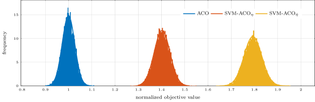
Figure 3: The distribution of the objective values generated by the ACO, SVM-ACO_η, and SVM-ACO${}_{\hat{\eta}}$ algorithms in the first iteration when tested on the orienteering problems of size $100$. The objective values are normalized by the mean objective value generated by ACO.

To show the efficacy of our ML prediction, we first compare the initial probabilistic models of SVM-ACO_η and SVM-ACO${}_{\hat{\eta}}$ against that of the classic ACO algorithm without ML enhancement. Note that the initial probabilistic model of SVM-ACO_τ is the same as that of SVM-ACO${}_{\hat{\eta}}$ under our parameter settings. Moreover, the initial probabilistic models of the two ACO variants, AS and MMAS are also identical. We use the initial probabilistic models to sample 10,000 solutions for each test problem instance, and plot the distribution of averaged normalized objective values in Figure 3. The objective values of the sample solutions are normalized by the mean objective value generated by the classic ACO algorithm. The normalized objective values are then averaged across 100 test problem instances. We can observe that the average objective values generated by SVM-ACO_η is about 40% better than that of the classic ACO algorithm without ML enhancement. The only difference between these two algorithms is that SVM-ACO_η sets $\eta_{i,j}$ based on predicted probability $p_{i,j}$, while ACO sets $\eta_{i,j}$ based on a heuristic rule $s_{j}/c_{i,j}$. In this sense, our ML prediction is more ‘greedy’ than the heuristic rule. Furthermore, by setting $\eta_{i,j}$ to the product of our predicted probability and the heuristic rule, the resulted algorithm SVM-ACO${}_{\hat{\eta}}$ improves over ACO by 80% in terms of the objective values generated in the first iteration.

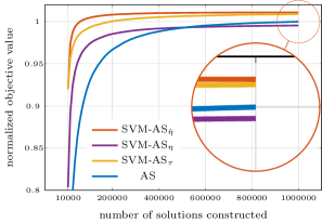
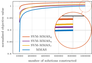
Figure 4: The convergence curves of the ACO (i.e., AS or MMAS), SVM-ACO_τ, SVM-ACO_η and SVM-ACO${}_{\hat{\eta}}$ algorithms when used to solve the orienteering problems of size $100$. The objective values are normalized by the best objective value found by ACO and are averaged across 100 instances.

We then compare the ACO algorithms (AS or MMAS) enhanced by ML prediction against the classic ACO algorithms, when solving the test problem instances. The number of solutions to be constructed is set to $10000n$ for each algorithm, where $n$ is problem dimensionality. The population size of AS is set to $100n$ and that of MMAS is $n$, because MMAS only uses a single best solution to update the pheromone matrix in each iteration, and thus it benefits more from relatively small population size and more iterations. The objective values generated by each algorithm are normalized by the best objective value found by AS (or MMAS), and are averaged across 100 problem instances and 25 independent runs. The curves of normalized objective value v.s. number of solutions constructed is shown in Figure 4. These convergence curves can show not only the final objective values generated by the algorithms but also their converging speed. We can observe that the performances of both AS and MMAS in finding high-quality solutions are greatly enhanced by ML prediction. Significantly, the solution generated by SVM-MMAS${}_{\hat{\eta}}$ at 4% of computational budget is already better than the final solution produced by MMAS. Furthermore, the enhanced AS and MMAS algorithms are generally able to find a better solution at the end of a run, except for the SVM-AS_η algorithm that may have an issue of premature convergence. We note that the hybridization SVM-ACO${}_{\hat{\eta}}$ works the best; it improves over the classic ACO by more than 1% in terms of the final solution quality generated. This improvement is larger if less computational budget is allowed. Hence, we will only employ the hybridization ($\hat{\eta}$) that sets $\eta_{i,j}=p_{i,j}\cdot s_{j}/c_{i,j}$ in the rest of the paper.

4.2 Sensitivity to machine learning algorithms

We take the SVM-ACO algorithm and replace SVM by LR and GCN to see if the performance of our hybrid algorithm is sensitive to the ML algorithm used in training. We train a separate model with LR and GCN on our training set. For GCN, we use 20 layers and each hidden layer has 32 neurons. The learning rate is set to $0.001$ and the number of epochs is $100$. The training time for LR is about $27$ seconds and that for GCN is about $1000$ seconds.

Similar as before, we compare the initial probabilistic models of the SVM-ACO, LR-ACO, GCN-ACO and ACO algorithms, and plot the distribution of objective values generated by each probabilistic model in Figure 5. We can observe that no matter which one of the three learning algorithms is used, the ACO enhanced by solution prediction significantly improves over the classic ACO by more than 50% in terms of the objective values generated in the first iteration. Among the three learning algorithms, the LR performs the worst and SVM is the best. This is a bit surprising as the simple linear SVM model performs slightly better than the deep GCN model in this context. Note that we have not done any fine-tuning for the GCN model, and we suspect that the performance of GCN may be further improved by tuning hyper-parameters. However, a thorough evaluation along this line requires significantly more computational resources and is beyond the scope of this paper.

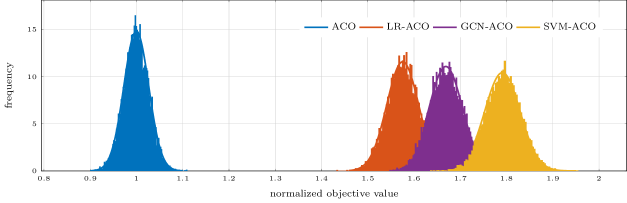
Figure 5: The distribution of objective values generated by the ACO, SVM-ACO, GCN-ACO, and LR-ACO algorithms in the first iteration when tested on the orienteering problems of size $100$. The objective values are normalized by the mean objective value generated by ACO.

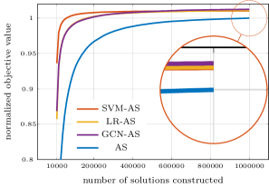
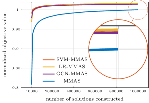
Figure 6: The convergence curves of the ACO (i.e., AS or MMAS), SVM-ACO, GCN-ACO, and LR-ACO algorithms when used to solve the orienteering problems of size $100$. The objective values are normalized by the best objective value found by ACO and are averaged across 100 instances.

We also compare the performance of the four algorithms for solving the test problem instances, and the averaged convergence curves are shown in Figure 6. The results show that the ACO algorithms (i.e., AS or MMAS) enhanced by different ML predictions consistently outperform the classic ACO in finding high-quality solutions. Whilst the initial objective values found by SVM-ACO, LR-ACO, and GCN-ACO are different, the final solutions generated by these algorithms are of a similar quality after many iterations of ACO sampling. In the rest of this paper, we will only use SVM as our ML model.

4.3 Generalization to larger problem instances

We test the generalization of our SVM-ACO algorithm to larger orienteering problem instances. To do so, we randomly generate larger problem instances with dimensionality 200, 300, 400 and 500, each with 100 problem instances, for testing. We then apply the SVM-ACO model, which is trained on small problem instances of dimensionality 50, to solve each of the larger test problem instance, compared against the classic ACO. The parameter settings for the two ACO variants, AS and MMAS are the same as before.

Table 1: The best objective values obtained by the AS, SVM-AS, MMAS and SVM-MMAS algorithms averaged across 100 problem instances in each problem set. A series of Wilcoxon signed-rank tests are performed between each pair of algorithms (i.e., AS vs SVM-AS and MMAS vs SVM-MMAS), and the p-values are reported. The statistically significantly better results are highlighted in bold (p-value $<$ 0.05).

Dataset	AS	SVM-AS	p-value	MMAS	SVM-MMAS	p-value
size 200	3043.22	3102.74	3.02e-12	3068.50	3254.87	3.39e-15
size 300	3674.04	3739.04	3.42e-12	3637.37	3944.72	8.86e-17
size 400	4278.65	4392.26	4.05e-15	4207.71	4665.61	4.01e-18
size 500	4752.65	4866.93	6.10e-14	4612.65	5167.52	1.05e-17

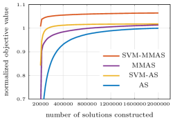
(a) size 200

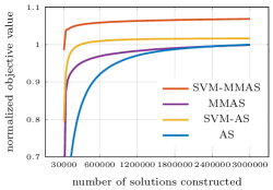
(b) size 300

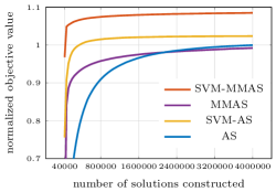
(c) size 400

(d) size 500

Figure 7: The convergence curves of the AS, SVM-AS, MMAS and SVM-MMAS algorithms, when used to solve the larger orienteering problem instances. The objective values are normalized by the best objective value found by AS and are averaged across 100 instances.

The best objective values obtained by each algorithm averaged across 100 problem instances for each problem set are presented in Table 1, and the averaged convergence curves are shown in Figure 7. First, we can observe that our ML model trained on small problem instances generalizes very well to larger test problem instances, in the sense that it consistently boosts the performance of both AS and MMAS when solving the larger problem instances. Furthermore, this improvement becomes more significant as the problem dimensionality increases from 200 to 500. The SVM-MMAS algorithm is clearly the best performing one among the four algorithms tested. Significantly, SVM-MMAS improves over MMAS by more than 10% in terms of the best objective values generated for the problem instances of dimensionality 500.

4.4 Generalization to benchmark problem instances

We evaluate the generalization capability of our SVM-ACO algorithm on a set of benchmark instances used in [Chao et al., 1996]. Each instance has 66 vertices, the locations of which form a square shape. The distance budget is varied from 5 to 130 in increments of 5, resulting in 26 instances in total. We apply the SVM-ACO algorithm, trained on randomly generated problem instances, to solve the square-shaped benchmark problem instances, compared against the classic ACO under the same parameter settings.

The averaged convergence curves of the algorithms when used to solve the benchmark problem instances are shown in Figure 8. The results show that our ML model trained on randomly generated instances generalizes well to the square-shaped benchmark instances. In particular, the SVM-MMAS algorithm is able to find a high-quality solution at the very early stage of the search process, comparing to MMAS. The mean and standard deviation of the best objective values generated by each algorithm across 25 runs for each problem instance are presented in Table 2. The statistically significantly better results obtained by the SVM-ACO and ACO algorithms are highlighted in bold, based on the Wilcoxon signed-rank tests with a significance level of 0.05. We can observe that on easy instances in which the distance budget is small, both the SVM-ACO and ACO algorithms are able to find the optimal solutions by the end of a run consistently. However, on hard instances in which the distance budget is large, the solution quality generated by SVM-ACO is statistically significantly better than that by the classic ACO algorithm.

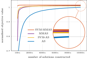
Figure 8: The convergence curves of the AS, SVM-AS, MMAS and SVM-MMAS algorithms, when used to solve the benchmark problem instances. The objective values are normalized by the best objective value found by AS and are averaged across 26 instances.

Table 2: The best objective values generated by the AS, SVM-AS, MMAS and SVM-MMAS algorithms on the benchmark problem instances. The statistically significantly better results generated by SVM-AS as opposed to AS (and SVM-MMAS as opposed to MMAS) are highlighted in bold, according to Wilcoxon signed-rank tests with a significance level of 0.05.

Datasets	Budget	AS		SVM-AS		MMAS		SVM-MMAS
		mean	std	mean	std	mean	std	mean	std
set_66_1_005	5	10.00	0.00	10.00	0.00	10.00	0.00	10.00	0.00
set_66_1_010	10	40.00	0.00	40.00	0.00	40.00	0.00	40.00	0.00
set_66_1_015	15	120.00	0.00	120.00	0.00	120.00	0.00	120.00	0.00
set_66_1_020	20	205.00	0.00	205.00	0.00	205.00	0.00	205.00	0.00
set_66_1_025	25	290.00	0.00	290.00	0.00	290.00	0.00	290.00	0.00
set_66_1_030	30	400.00	0.00	400.00	0.00	400.00	0.00	400.00	0.00
set_66_1_035	35	465.00	0.00	465.00	0.00	465.00	0.00	465.00	0.00
set_66_1_040	40	575.00	0.00	575.00	0.00	575.00	0.00	575.00	0.00
set_66_1_045	45	647.60	2.55	649.20	1.87	648.60	2.29	650.00	0.00
set_66_1_050	50	730.00	0.00	730.00	0.00	729.20	3.12	730.00	0.00
set_66_1_055	55	820.40	2.00	823.60	3.39	823.00	2.50	824.80	1.00
set_66_1_060	60	904.80	6.84	910.20	5.68	914.20	2.36	915.00	0.00
set_66_1_065	65	972.40	5.02	976.60	5.72	980.00	0.00	980.00	0.00
set_66_1_070	70	1055.00	8.42	1065.20	8.72	1069.60	1.38	1070.00	0.00
set_66_1_075	75	1126.00	9.46	1138.60	4.45	1140.00	0.00	1140.00	0.00
set_66_1_080	80	1188.20	10.09	1206.80	8.52	1209.20	6.24	1215.00	0.00
set_66_1_085	85	1242.80	6.47	1265.20	6.84	1264.60	3.20	1270.00	0.00
set_66_1_090	90	1302.60	9.03	1322.80	10.91	1329.80	6.84	1340.00	0.00
set_66_1_095	95	1354.20	10.58	1379.40	10.24	1386.60	6.25	1394.80	1.00
set_66_1_100	100	1405.60	8.33	1436.40	11.23	1447.20	9.36	1464.60	2.00
set_66_1_105	105	1452.00	11.64	1484.40	10.64	1508.20	8.65	1519.20	2.77
set_66_1_110	110	1496.60	10.48	1529.60	9.46	1549.40	7.82	1560.00	0.00
set_66_1_115	115	1544.00	10.80	1576.80	9.45	1583.80	8.07	1594.80	1.00
set_66_1_120	120	1582.40	8.55	1617.40	9.03	1623.00	8.29	1634.60	2.00
set_66_1_125	125	1615.40	6.91	1654.60	9.46	1654.60	5.94	1670.00	0.00
set_66_1_130	130	1649.40	5.83	1675.80	4.72	1675.00	3.82	1680.00	0.00

4.5 Generalization to real-world problem instances

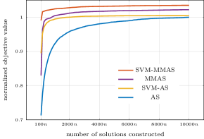
Figure 9: The convergence curves of the AS, SVM-AS, MMAS and SVM-MMAS algorithms, when used to solve the real-world problem instances. The objective values are normalized by the best objective value found by AS and are averaged across six instances.

Table 3: The best objective values generated by the AS, SVM-AS, MMAS and SVM-MMAS algorithms on the real-world problem instances. The statistically significantly better results generated by SVM-AS as opposed to AS (and SVM-MMAS as opposed to MMAS) are highlighted in bold, according to Wilcoxon signed-rank tests with a significance level of 0.05.

Datasets	Dimension	AS		SVM-AS		MMAS		SVM-MMAS
		mean	std	mean	std	mean	std	mean	std
Berlin	97	188.39	1.08	191.00	1.70	192.63	0.93	195.46	0.64
Copenhagen	81	227.28	1.90	228.01	2.14	232.21	1.61	235.62	1.79
Istanbul	154	206.11	1.68	208.36	1.79	209.11	1.25	215.12	1.25
London	114	172.88	0.92	172.52	0.70	175.82	0.64	176.02	1.52
Paris	117	153.81	0.76	153.47	2.21	158.83	1.41	159.19	1.78
Prague	78	242.73	1.34	244.52	1.62	248.48	1.26	251.73	1.20

We further test the generalization of our SVM-ACO algorithm to real-world problem instances – tourist trip planning, where the goal is to plan an itinerary that visits a subset of attractions in a city within a given distance (or time) budget such that the total collected ‘popularity score’ is maximized. We use six datasets published in a trajectory-driven tourist trip planning system [Wang et al., 2018] to test our model. Each dataset corresponds to a city in Europe. The starting and ending vertex of a dataset is a hotel randomly chosen from the corresponding city, and the other vertices are attractions for visiting. The coordinates of each vertex are its geographic location: latitude and longitude; and the distance between two vertices is the geographical distance between them. The popularity score of an attraction is calculated based on how many people have visited that attraction: $s_{i}=\log_{2}(n_{i}+1)$, where $n_{i}$ is the number of trajectories that have been to that attraction. The trajectory data was originally crawled from the Triphobo website by Wang et al. [Wang et al., 2018]. The dimensionality of these six datasets varies from 81 to 154. The total distance budget is set to 50 kilometers for each dataset. We take the SVM-ACO model trained on synthetic problem instances and test it on these real-world problem instances.

The average convergence curves of the AS, SVM-AS, MMAS and SVM-MMAS algorithms when used to solve the real-world problem instances are shown in Figure 9. The results show that our ML model trained on synthetic problem instances generalizes well to real-world problem instances; the ML model speeds up both AS and MMAS in finding high-quality solutions for the real-world instances. Overall, the SVM-MMAS algorithm achieves the best solution quality, and improves over MMAS by 1.24% on average. The mean and standard deviation of the best objective values generated by each algorithm across 25 runs for each problem instance are presented in Table 3. We can see that both AS and MMAS consistently find an equally well or statistically significantly better solution when enhanced by our ML prediction.

4.6 Comparison with state-of-the-art algorithms

We take the best-performing algorithm SVM-MMAS and compare it against three state-of-the-art heuristics, Evolutionary Algorithm for Orienteering Problem (EA4OP) [Kobeaga et al., 2018], GRASP with Path Relinking (GRASP-PR) [Campos et al., 2014] and 2-Parameter Iterative Algorithm (2P-IA) [Silberholz & Golden, 2010]. These three state-of-the-art algorithms all use effective local search methods. For a fair comparison, we also use a local search method to improve the solutions sampled by SVM-MMAS. Specifically, we use the well-known 2-opt local search method [Lin, 1965] to reduce the path length of the best solution constructed in each iteration of SVM-MMAS. Candidate vertices (i.e., those have not been visited) are greedily inserted into the path until a local optimum is found. Note that the 2-opt local search method is repeatedly applied when a candidate vertex is inserted into the path, attempting to reduce the path length.

We compare the performance of our algorithm (denoted as SVM-MMAS-LS) with the state-of-the-art heuristics on a set of benchmark problem instances [Fischetti et al., 1998], of which the number of vertices ranges from 48 to 400. These instances (generation 3) were generated based on the TSP library, and are available from the OP library (https://github.com/bcamath-ds/OPLib). For each problem instance, we run our SVM-MMAS-LS algorithm 10 times, and record the best solution found and the average runtime used, following [Kobeaga et al., 2018]. The parameters of our algorithm are set as before with four exceptions:

1. We use a different termination criterion for our SVM-MMAS-LS algorithm, i.e., if the best solution found cannot be improved for $T_{\mathrm{ter}}$ consecutive iterations, the algorithm is terminated. We will test two different values for $T_{\mathrm{ter}}$: 200 and 500.

2. We have tested the use of both the iteration-best solution and the global-best solution to update the pheromone matrix, and found that using the global-best solution can generate an optimality gap that is 44% better than that of using the iteration-best solution on average. Therefore, we will use the global-best solution to update the pheromone matrix.

3. We have tested three different population sizes {50, 100, $n$} and found that using a larger population size can generate a slightly smaller optimality gap but significantly increases the runtime. Hence, we will set the population size to 50.

4. We use the SVM model (primal formulation) implemented in the LIBLINEAR library, which is faster than that of the LIBSVM library (dual formulation) in prediction. Furthermore, we reduce the sample size $m$ to $10n$, to gain computational efficiency.

The results are presented in Table 4. Note that the results of EA4OP, GRASP-PR and 2P-IA are taken from Table A.5 of [Kobeaga et al., 2018]. We can observe that our SVM-MMAS-LS algorithm with $T_{\mathrm{ter}}=200$ is already competitive with the three state-of-the-art heuristics. On average, SVM-MMAS-LS achieves a smaller optimality gap than the other three algorithms using similar runtime (see the last row of Table 4). When $T_{\mathrm{ter}}$ is increased from 200 to 500, the average optimality gap can be further reduced, but at an expense of longer runtime.

Finally, we would like to remark that our primary aim is not to develop the best algorithm for solving the orienteering problem. Instead, our aim is to boost the performance of ACO via solution prediction and ML. Therefore, our experiments have mainly focused on showing whether the ML-enhanced ACO algorithm outperforms the classic ACO. In fact, our ML-enhanced ACO is not confined to solving the orienteering problem. In Appendix B, we adapt our ML-enhanced ACO algorithm to solve the maximum weighted clique problem and show that it is competitive compared to the state-of-the-art algorithms.

Table 4: The comparison between our SVM-MMAS-LS algorithm and three state-of-the-art heuristics on a set of benchmark problem instances. The column ‘Opt’ presents the optimal objective value. For each algorithm, the best objective value found, optimality gap (%) and the average time used (in second) are presented. The best optimality gap is highlighted in bold.

Instance	Opt	2P-IA			GRASP-PR			EA4OP			SVM-MMAS-LS (200)			SVM-MMAS-LS (500)
		best	gap	time	best	gap	time	best	gap	time	best	gap	time	best	gap	time
att48	1049	1049	0.00	0.13	1049	0.00	0.18	1049	0.00	0.26	1049	0.00	0.22	1049	0.00	0.39
gr48	1480	1480	0.00	0.07	1480	0.00	0.20	1480	0.00	0.13	1480	0.00	0.21	1480	0.00	0.43
hk48	1764	1764	0.00	0.09	1764	0.00	0.14	1764	0.00	0.22	1764	0.00	0.23	1764	0.00	0.36
eil51	1399	1399	0.00	0.12	1399	0.00	0.17	1398	0.07	0.22	1399	0.00	0.25	1399	0.00	0.50
berlin52	1036	1036	0.00	0.19	1036	0.00	0.30	1034	0.19	0.64	1036	0.00	0.20	1036	0.00	0.39
brazil58	1702	1702	0.00	0.13	1702	0.00	0.33	1702	0.00	0.71	1702	0.00	0.29	1702	0.00	0.48
st70	2108	2108	0.00	0.24	2108	0.00	0.37	2108	0.00	0.31	2108	0.00	0.36	2108	0.00	0.79
eil76	2467	2461	0.24	0.30	2462	0.20	0.44	2467	0.00	0.36	2462	0.20	0.51	2467	0.00	1.05
pr76	2430	2430	0.00	0.26	2430	0.00	0.56	2430	0.00	0.57	2430	0.00	0.48	2430	0.00	1.12
gr96	3170	3170	0.00	0.39	3153	0.54	1.07	3166	0.13	1.41	3170	0.00	0.93	3170	0.00	1.49
rat99	2908	2896	0.41	0.47	2881	0.93	0.80	2886	0.76	0.78	2870	1.31	0.54	2908	0.00	1.32
kroA100	3211	3211	0.00	0.30	3211	0.00	1.16	3180	0.97	0.38	3206	0.16	0.76	3211	0.00	1.69
kroB100	2804	2804	0.00	0.46	2804	0.00	1.34	2785	0.68	0.51	2804	0.00	0.64	2804	0.00	1.29
kroC100	3155	3155	0.00	0.38	3149	0.19	0.86	3155	0.00	0.44	3149	0.19	0.70	3140	0.48	1.20
kroD100	3167	3123	1.39	0.65	3167	0.00	1.18	3141	0.82	0.58	3147	0.63	0.58	3151	0.51	1.55
kroE100	3049	3027	0.72	0.56	3049	0.00	1.48	3049	0.00	0.47	3049	0.00	0.58	3049	0.00	1.15
rd100	2926	2924	0.07	0.62	2924	0.07	0.90	2923	0.10	0.48	2926	0.00	0.71	2926	0.00	1.85
eil101	3345	3333	0.36	0.46	3322	0.69	0.76	3345	0.00	0.56	3335	0.30	0.92	3322	0.69	2.02
lin105	2986	2986	0.00	0.54	2986	0.00	1.89	2973	0.44	2.09	2986	0.00	0.68	2986	0.00	1.92
pr107	1877	1877	0.00	0.29	1877	0.00	1.15	1802	4.00	0.82	1875	0.11	0.46	1877	0.00	0.76
gr120	3779	3736	1.14	0.96	3745	0.90	1.15	3748	0.82	1.36	3687	2.43	1.23	3765	0.37	3.07
pr124	3557	3517	1.12	0.62	3549	0.22	2.41	3455	2.87	0.88	3549	0.22	0.98	3549	0.22	1.63
bier127	2365	2356	0.38	1.08	2332	1.40	2.07	2361	0.17	2.62	2336	1.23	1.57	2347	0.76	3.62
pr136	4390	4390	0.00	0.93	4380	0.23	2.56	4390	0.00	1.13	4312	1.78	1.31	4299	2.07	2.85
gr137	3954	3928	0.66	1.13	3926	0.71	1.89	3954	0.00	1.88	3932	0.56	1.80	3934	0.51	2.64
pr144	3745	3633	2.99	0.77	3745	0.00	3.36	3700	1.20	2.41	3745	0.00	0.96	3745	0.00	2.11
kroA150	5039	5037	0.04	1.26	5018	0.42	3.06	5019	0.40	1.07	5011	0.56	1.56	5034	0.10	3.71
kroB150	5314	5267	0.88	1.31	5272	0.79	2.31	5314	0.00	1.04	5177	2.58	1.68	5253	1.15	4.12
pr152	3905	3557	8.91	0.80	3905	0.00	4.07	3902	0.08	3.62	3905	0.00	1.37	3905	0.00	2.85
u159	5272	5272	0.00	1.33	5272	0.00	4.46	5272	0.00	0.94	5214	1.10	1.48	5218	1.02	3.97
rat195	6195	6174	0.34	2.22	6086	1.76	3.06	6139	0.90	2.00	6127	1.10	3.00	6125	1.13	6.46
d198	6320	5985	5.30	1.86	6162	2.50	5.86	6290	0.47	7.14	6258	0.98	2.71	6212	1.71	5.46
kroA200	6123	6048	1.22	2.73	6084	0.64	4.64	6114	0.15	1.72	5971	2.48	2.39	6028	1.55	7.14
kroB200	6266	6251	0.24	2.79	6190	1.21	5.46	6213	0.85	1.77	6163	1.64	3.17	6226	0.64	4.78
gr202	8616	8111	5.86	2.05	8419	2.29	9.12	8605	0.13	10.45	8464	1.76	3.79	8542	0.86	9.68
ts225	7575	7149	5.62	1.47	7510	0.86	6.15	7575	0.00	1.14	7486	1.17	3.12	7575	0.00	9.80
tsp225	7740	7353	5.00	2.38	7565	2.26	5.04	7488	3.26	2.58	7607	1.72	3.74	7681	0.76	11.50
pr226	6993	6652	4.88	1.97	6964	0.41	15.50	6908	1.22	8.01	6950	0.61	3.37	6937	0.80	6.10
gr229	6328	6190	2.18	4.42	6205	1.94	9.03	6297	0.49	11.65	6135	3.05	5.98	6197	2.07	17.40
gil262	9246	8915	3.58	5.68	8922	3.50	6.07	9094	1.64	3.94	9090	1.69	7.57	9116	1.41	22.60
pr264	8137	7820	3.90	3.98	7959	2.19	17.88	8068	0.85	3.62	8118	0.23	4.21	8086	0.63	7.44
a280	9774	8719	10.79	4.53	9426	3.56	9.42	8684	11.15	3.22	9609	1.69	4.83	9587	1.91	13.55
pr299	10343	10305	0.37	6.07	10033	3.00	19.61	9959	3.71	3.95	10227	1.12	5.40	10254	0.86	16.01
lin318	10368	9909	4.43	7.57	9758	5.88	12.18	10273	0.92	6.33	10155	2.05	9.05	10271	0.94	21.95
rd400	13223	12828	2.99	14.49	12678	4.12	16.46	13088	1.02	7.74	12552	5.07	12.15	12848	2.84	53.39
average	4724	4601	1.69	1.80	4646	0.96	4.18	4661	0.90	2.31	4661	0.88	2.19	4683	0.58	5.90

5 Conclusion

We have proposed a new meta-heuristic called ML-ACO that integrates machine learning (ML) with ant colony optimization (ACO) to solve the orienteering problem. Our ML model trained on optimally-solved problem instances, is able to predict which edges in the graph of a test problem instance are more likely to be part of the optimal route. We incorporated the ML predictions into the probabilistic model of ACO to bias its sampling towards using the predicted ‘high-quality’ edges more often when constructing solutions. This in turn significantly boosted the performance of ACO in finding high-quality solutions for a test problem instance. We tested three different classification algorithms, and the experimental results showed that all of the ML-enhanced ACO variants significantly improved the classic ACO in terms of both speed of convergence and quality of the final solution. Of the three ML models, the SVM based predictions produced the best results for this application. The best results were obtained by using the prediction to modify the heuristic weights rather than just for the initial pheromone matrix. Importantly, our ML model trained on small synthetic problem instances generalized very well to large synthetic and real-world problem instances.

We see great potential of the integration between ML (more specifically solution prediction) and meta-heuristics, and a lot of opportunities for future work. First, there is a large family of meta-heuristics, that can potentially be improved by solution prediction. Second, it would be interesting to see if this integrated technique also works on other combinatorial optimization problems as well as continuous, dynamic or multi-objective optimization problems. In particular, we expect this integrated technique would be more effective in solving a dynamic problem where the optimal solution changes over time. Based on the results shown in this paper, solution prediction is very greedy, and therefore can potentially adapt quickly to any changes occurring in a problem. Third, there is a large number of ML algorithms that can be used for solution prediction. Meta-heuristics will certainly benefit more from this type of hybridization, if we can further improve the accuracy of solution prediction. This paper shows that SVM, one of the simpler ML models, is already highly effective. However, given the large number of advanced ML methods developed in recent years, there may be others that are even more effective in this context of boosting meta-heuristics.

A Supplementary Methodology

A.1 A random sampling method for the orienteering problem

Consider an orienteering problem instance $G(V,E,S,C)$ with a given time budget $T_{\mathrm{max}}$. Without loss of generality, we assume $v_{1}$ is the starting vertex and $v_{n}$ is the ending vertex. The main steps of our random sampling method to generate one feasible solution (route) are:

1. Initialize a route with the starting vertex $v_{1}$;

2. Generate a random permutation of the candidate vertices $\{v_{2},\ldots,v_{n-1}\}$ that can be visited;

3. Consider the vertices in the generated permutation one by one, and add the vertices to the sample route which does not violate the time budget constraint;

4. Add the ending vertex $v_{n}$ to the sample route.

The pseudocode of the random sampling method is presented in Algorithm 1. It is obvious that the time complexity of generating one sample route by using this method is $\mathcal{O}(n)$, where $n$ is the number of vertices in a problem instance. Hence, the total time complexity of generating $m$ sample routes is $\mathcal{O}(mn)$. Furthermore, the sample size $m$ should be larger than $n$; otherwise there will be some edges that are never sampled. This is because the number of edges in the directed complete graph is $n(n-1)$, and the total number of edges in $m$ sample routes is no more than $mn$. Therefore, each edge is expected to be sampled no more than $m/(n-1)$ times.

Algorithm 1 Random Sampling Method

1:vertex set $V$, vertex score set $S$, edge cost set $C$, time budget $T_{\mathrm{max}}$, number of samples to generate $m$.

2:for $k$ from $1$ to $m$ do

3:     Initialize the route $P^{k}$ with the starting vertex $v_{1}$;

4:     Initialize the object value $y^{k}\leftarrow S[v_{1}]$;

5:     Initialize the current vertex $v_{c}\leftarrow v_{1}$;

6:     Initialize the time used so far $t_{c}\leftarrow 0$;

7:     Generate a random permutation of $\{v_{2},\ldots,v_{n-1}\}$;

8:     for $v_{j}$ in the generated random permutation do

9:         if $t_{c}+C[v_{c},v_{j}]+C[v_{j},v_{n}]\leq T_{\mathrm{max}}$ then

10:              Add $v_{j}$ to the route $P_{k}$;

11:              Update $y^{k}\leftarrow y^{k}+S[v_{j}]$;

12:              Update $t_{c}\leftarrow t_{c}+C[v_{c},v_{j}]$;

13:              Update $v_{c}\leftarrow v_{j}$;               

14:     Add $v_{n}$ to the route $P_{k}$;

15:     Update $y^{k}\leftarrow y^{k}+S[v_{n}]$;

16:return $\{P^{1},\ldots,P^{m}\}$ and $\{y^{1},\ldots,y^{m}\}$.

A.2 An efficient method for computing the statistical measures

In the main paper, we used a binary string $\bm{x}$ to represent a sample solution (route), where $x_{i,j}=1$ if the edge $e_{i,j}$ is in the route; otherwise $x_{i,j}=0$. We have shown that directly computing the ranking-based measure and correlation-based measure based on the binary string representation $\bf{x}$ costs $\mathcal{O}(mn^{2})$. Here, we adapt the method proposed in [Sun et al., 2021b] to efficiently compute the two statistical measures based on set representation $P$, which only stores the edges appearing in the corresponding sample route.

Let $\{P^{1},\ldots,P^{m}\}$ be the set representation of the $m$ randomly generated solutions; $\{\bm{x}^{1},\ldots,\bm{x}^{m}\}$ be the corresponding binary string representation; and $\{y^{1},\ldots,y^{m}\}$ be their objective values. Because $x_{i,j}^{k}$ are binary variables, we can simplify the calculation of Pearson correlation coefficient by using the following two equalities:

$$\sum_{k=1}^{m}(x_{i,j}^{k}-\bar{x}_{i,j})^{2}=\bar{x}_{i,j}(1-\bar{x}_{i,j})m,$$ (22)

$$\sum_{k=1}^{m}(x_{i,j}^{k}-\bar{x}_{i,j})(y^{k}-\bar{y})=(1-\bar{x}_{i,j})s_{i,j}^{1}-\bar{x}_{i,j}s_{i,j}^{0},$$ (23)

where $\bar{x}_{i,j}=\sum_{k=1}^{m}x_{i,j}^{k}/m$, $\bar{y}=\sum_{k=1}^{m}y^{k}/m$ and

$$s_{i,j}^{1}=\mathop{\sum\limits_{1\leq k\leq m}}\limits_{x_{i,j}^{k}=1}(y^{k}-\bar{y});\;\text{and}\;s_{i,j}^{0}=\mathop{\sum\limits_{1\leq k\leq m}}\limits_{x_{i,j}^{k}=0}(y^{k}-\bar{y}).$$ (24)

The proof of these two equalities can be found in [Sun et al., 2021b]. We then are able to compute the two statistical measures in $\mathcal{O}(mn+n^{2})$ by using Algorithm 2. Computing our ranking-based measure $f_{r}$ based on the set representation is straightforward, i.e., scanning through the edges in each sample route $P$ to accumulate the rankings. To compute the correlation-based measure, we first iterate through the edges in each sample route $P$ to accumulate $\bar{x}_{i,j}$ and $s_{i,j}^{1}$, i.e., line 7 to 12 in Algorithm 2. Our correlation-based measure $f_{c}$ can then be easily computed based on $\bar{x}_{i,j}$ and $s_{i,j}^{1}$ (line 13 to 17 in Algorithm 2).

Algorithm 2 Computing Statistical Measures

1:samples $\mathbb{P}$, objective values $Y$, number of samples $m$, number of vertices $n$, and edge set $E$.

2:Sort the samples in $\mathbb{P}$ based on objective value $Y$; and use $r^{k}$ to denote the ranking of $k^{\mathrm{th}}$ sample $P^{k}$;

3:Compute mean objective value: $\bar{y}\leftarrow\sum_{k=1}^{m}y^{k}/m$;

4:Compute objective difference: $y_{d}\leftarrow\sum_{k=1}^{m}(y^{k}-\bar{y})$;

5:Compute objective variance: $\sigma_{y}\leftarrow\sum_{k=1}^{m}(y^{k}-\bar{y})^{2}$;

6:Initialize $f_{r}$, $\bar{x}_{i,j}$ and $s_{i,j}^{1}$ to $0$, for each $e_{i,j}\in E$;

7:for $k$ from $1$ to $m$ do

8:     for $idx$ from $1$ to $|P^{k}|-1$ do

9:         $i\leftarrow P^{k}[idx]$, $j\leftarrow P^{k}[idx+1]$;

10:         $f_{r}(e_{i,j})\leftarrow f_{r}(e_{i,j})+1/r^{k}$;

11:         $\bar{x}_{i,j}\leftarrow\bar{x}_{i,j}+1/m$;

12:         $s_{i,j}^{1}\leftarrow s_{i,j}^{1}+(y^{k}-\bar{y})$;      

13:for $i$ from $1$ to $n$ do

14:     for $j$ from $1$ to $n$ and $j\neq i$ do

15:         $\sigma_{c_{i,j}}\leftarrow(1-\bar{x}_{i,j})s_{i,j}^{1}-\bar{x}_{i,j}(y_{d}-s_{i,j}^{1})$;

16:         $\sigma_{x_{i,j}}\leftarrow\bar{x}_{i,j}(1-\bar{x}_{i,j})m$;

17:         $f_{c}(e_{i,j})\leftarrow\sigma_{c_{i,j}}/\sqrt{\sigma_{x_{i,j}}\sigma_{y}}$;      

18:return $f_{r}$ and $f_{c}$.

A.3 A brief introduction of the machine learning algorithms used

Support Vector Machine (SVM): Given a training set $\mathbb{S}=\{(\bm{f}^{i},l^{i})\,|\,i=1,\ldots,n_{t}\}$, the aim of SVM is to find a decision boundary ($\bm{w}^{T}\bm{f}+b=0$) in the feature space to maximize the so-called geometric margin, defined as the smallest distance from a training point to the decision boundary [Boser et al., 1992, Cortes & Vapnik, 1995]. We use an L2-regularized linear SVM model, that finds the optimal decision boundary by solving the following quadratic programming with linear constraints:

$$\min_{\bm{w},b,\bm{\xi}} \quad\frac{1}{2}\bm{w}^{T}\bm{w}+r^{+}\sum_{l^{i}=1}\xi^{i}+r^{-}\sum_{l^{i}=-1}\xi^{i},$$ (25)

$$s.t. \quad l^{i}\big{(}\bm{w}^{T}\bm{f}^{i}+b\big{)}\geq 1-\xi^{i},\quad i=1,\ldots n_{t},$$ (26)

$$\quad\xi^{i}\geq 0,\quad i=1,\ldots n_{t},$$ (27)

where $r^{+}>0$ and $r^{-}>0$ are the regularization parameters for positive and negative training points; and $\xi^{i}$, $i=1,\ldots,n_{t}$ are slack variables.

Logistic Regression (LR) uses a loss function derived from the logistic function $g(x)=1/(1+e^{-x})$, whose output is in between $[0,1]$ and can be interpreted as probability. LR aims to separate positive and negative training points by maximum likelihood estimation [Bishop, 2006]. We use an L2-regularized LR model that fits its parameters ($\bm{w}$, $b$) by solving the following optimization problem:

$$\min_{\bm{w},b}\quad\frac{1}{2}\bm{w}^{T}\bm{w}+r^{+}\sum_{l^{i}=1}\log_{2}(1+e^{-\bm{w}^{T}\bm{f}^{i}-b})+r^{-}\sum_{l^{i}=-1}\log_{2}(1+e^{\bm{w}^{T}\bm{f}^{i}+b}).$$ (28)

Graph Convolutional Network (GCN) is a convolutional neural network that makes use of graph structure when classifying vertices in a graph [Kipf & Welling, 2017]. Consider a simple GCN model with only two layers: the input layer contains feature vectors $\bm{f}$ and the output layer is a predicted scalar $z$ for a vertex in a graph. To compute $z_{i}$ for vertex $v_{i}$ in a graph, GCN aggregates its feature vector $\bm{f}^{i}$ with that of its neighbours $\mathcal{N}_{i}$:

$$z_{i}=\bm{w}_{0}\bm{f}^{i}+\bm{w}_{1}\sum_{v_{j}\in\mathcal{N}_{i}}\sqrt{d_{i}d_{j}}\bm{f}^{j},$$ (29)

where $d_{i}$ and $d_{j}$ are the degrees of vertex $v_{i}$ and $v_{j}$; $\bm{w}_{0}$ and $\bm{w}_{1}$ are the weights to be optimized. This two-layer GCN model is a simple linear classifier, which is not expected to work well in practice. Thus, we usually use multiple hidden layers between the input and output layers, and each hidden layer can have multiple ‘neurons’. A hidden layer basically takes the output of its previous layer as input, and performs a linear transformation of its input. The intermediate output of the linear transformation is then filtered by an activation function to make GCN a non-linear classifier. In our experiments, the GCN model consists of 20 layers and each hidden layer has 32 neurons. The activation function used is the ReLU function [Nair & Hinton, 2010], defined as $\text{ReLU}(x)=\max(0,x)$. The weights ($\bm{w}$) of GCN are optimized via stochastic gradient descent with L2-regularized cross-entropy loss function [Kipf & Welling, 2017]. In the case of binary classification, the cross-entropy loss function is identical to the loss function of the LR algorithm:

$$\min_{\bm{w}}\quad\frac{1}{2}\bm{w}^{T}\bm{w}+r^{+}\sum_{l^{i}=1}\log_{2}(1+e^{-z_{i}})+r^{-}\sum_{l^{i}=-1}\log_{2}(1+e^{z_{i}}),$$ (30)

where $\bm{w}$ is a vector of all GCN’s weights to be optimized, and $z_{i}$ is the output (prediction) of GCN for the $i^{\mathrm{th}}$ training point. Because our training points are edges instead of vertices in the graphs of the orienteering problem instances, the GCN model cannot be directly applied to make predictions for edges in the graphs. To tackle this, we transfer the original graph ($G$) to its line graph ($\bar{G}$) such that the edges in $G$ are now vertices in $\bar{G}$ and the neighbouring edges (i.e., edges sharing a common vertex) in $G$ are now neighbouring vertices (i.e., vertices sharing a common edge) in $\bar{G}$. We then can apply the GCN model on the line graph $\bar{G}$ to make predictions for the edges in the original graph $G$.

B Adapting ML-ACO to Solve the Maximum Weighted Clique Problem

As our ML-ACO algorithm is a generic approach, we apply it to solve another combinatorial optimization problem, the maximum weighted clique problem (MWCP). The MWCP is a variant of the maximum clique problem, which is a fundamental problem in graph theory with a wide range of real-world applications [Wu & Hao, 2015, Malladi et al., 2017, Letchford et al., 2020, Blum et al., 2021]. Solving the MWCP is NP-hard, and a large number of solution methods have been developed for this problem recently. These include exact solvers such as branch-and-bound algorithms [Jiang et al., 2017, 2018, Li et al., 2018a, San Segundo et al., 2019] and local search methods [Wang et al., 2016, Cai & Lin, 2016, Zhou et al., 2017, Nogueira & Pinheiro, 2018, Wang et al., 2020].

Here, the aim of our ML model is to predict the ‘probability’ of a vertex being part of the maximum weighted clique. To train our ML model, we construct a training set using eighteen optimally-solved small graphs ($|V|<1000$) from the standard DIMACS library. The original DIMACS graphs are unweighted, and thus we assign a weight $w_{i}=(i\mod 200)+1$ to the vertex $v_{i}$ $(i=1,\ldots,|V|)$, following the previous works [Wang et al., 2016, Cai & Lin, 2016, Jiang et al., 2017, 2018]. Each training instance corresponds to a vertex in a training graph. We extract six features to characterize a vertex, including graph density, vertex weight, vertex degree, an upper bound and two statistical features described in [Sun et al., 2021b]. A training instance is labeled as $1$ if the corresponding vertex belongs to the maximum weighted clique; otherwise it is labeled as $-1$. We then train a linear SVM to classify whether a vertex belongs to the maximum weighted clique or not.

We use fifteen larger graphs ($|V|\geq 1000$) from the DIMACS library as our test problem instances. For each problem instance, we use the trained ML model to predict a probability value $p_{i}$ for each vertex $v_{i}\in V$. The predicted values ($p_{i}$) are then incorporated into the MMAS algorithm to guide its sampling towards larger-weighted cliques. More specifically, we use $p_{i}$ to set the heuristic weight: $\eta_{i}=p_{i}\cdot w_{i}$, for each $v_{i}\in V$. The parameter settings for MMAS and linear SVM are the same as before. We compare our ML-ACO algorithm against two exact solvers – TSM [Jiang et al., 2018] and WLMC [Jiang et al., 2017] as well as two heuristic methods LSCC [Wang et al., 2016] and FastWClq [Cai & Lin, 2016] for solving the MWCP. The cutoff time for each algorithm is set to 1000 seconds.

The best objective values obtained by each algorithm in 25 independent runs are presented in Table 5. We can observe that our ML-ACO algorithm is comparable to the state-of-the-art algorithms for solving the MWCP. On average, the best objective values found by our ML-ACO algorithm are significantly better than those found by FastWClq, WLMC and TSM. The LSCC algorithm performs the best and generates slightly better results than our ML-ACO algorithm. These results are interesting, because generic solution methods such as our ML-ACO algorithm are not often expected to be as competitive as specialized solvers.

Table 5: The best objective values generated by our ML-ACO algorithm and four state-of-the-arts for solving the MWCP. The best results are highlighted in bold.

Graph	$|V|$	ML-ACO	FastWClq	LSCC	WLMC	TSM
p_hat1000-1	1000	1514	1514	1514	1514	1514
p_hat1000-2	1000	5777	5777	5777	5777	5777
p_hat1000-3	1000	8111	8058	8111	8076	8111
p_hat1500-1	1500	1619	1619	1619	1619	1619
p_hat1500-2	1500	7360	7327	7360	7360	7360
p_hat1500-3	1500	10321	10057	10321	9846	10119
DSJC1000.5	1000	2186	2186	2186	2186	2186
san1000	1000	1716	1716	1716	1716	1716
C1000.9	1000	9191	8685	9254	7317	7341
C2000.5	2000	2466	2466	2466	2360	2407
C2000.9	2000	10888	9943	10964	7738	8228
C4000.5	4000	2776	2645	2792	2383	2402
MANN_a45	1035	34209	34111	34243	34265	34259
hamming10-2	1024	50512	50512	50512	50512	50512
hamming10-4	1024	5127	4982	5129	4738	4812
average	-	10252	10107	10264	9827	9891

References

- Abadi et al. [2015] Abadi, M., Agarwal, A., Barham, P. et al. (2015). TensorFlow: Large-scale machine learning on heterogeneous systems. URL: https://www.tensorflow.org/ software available from tensorflow.org.
- Abbasi et al. [2020] Abbasi, B., Babaei, T., Hosseinifard, Z., Smith-Miles, K., & Dehghani, M. (2020). Predicting solutions of large-scale optimization problems via machine learning: A case study in blood supply chain management. Computers & Operations Research, 119, 104941.
- Angelelli et al. [2017] Angelelli, E., Archetti, C., Filippi, C., & Vindigni, M. (2017). The probabilistic orienteering problem. Computers & Operations Research, 81, 269–281.
- Archetti et al. [2016] Archetti, C., Corberán, Á., Plana, I., Sanchis, J. M., & Speranza, M. G. (2016). A branch-and-cut algorithm for the orienteering arc routing problem. Computers & Operations Research, 66, 95–104.
- Assunção & Mateus [2021] Assunção, L., & Mateus, G. R. (2021). Coupling feasibility pump and large neighborhood search to solve the steiner team orienteering problem. Computers & Operations Research, 128, 105175.
- Bengio et al. [2021] Bengio, Y., Lodi, A., & Prouvost, A. (2021). Machine learning for combinatorial optimization: a methodological tour d’horizon. European Journal of Operational Research, 290, 405–421.
- Bishop [2006] Bishop, C. M. (2006). Pattern Recognition and Machine Learning. Springer.
- Blum [2005] Blum, C. (2005). Ant colony optimization: Introduction and recent trends. Physics of Life Reviews, 2, 353–373.
- Blum et al. [2021] Blum, C., Djukanovic, M., Santini, A., Jiang, H., Li, C.-M., Manyà, F., & Raidl, G. R. (2021). Solving longest common subsequence problems via a transformation to the maximum clique problem. Computers & Operations Research, 125, 105089.
- Boser et al. [1992] Boser, B. E., Guyon, I. M., & Vapnik, V. N. (1992). A training algorithm for optimal margin classifiers. In Proceedings of the Fifth Annual Workshop on Computational Learning Theory (pp. 144–152).
- Cai & Lin [2016] Cai, S., & Lin, J. (2016). Fast solving maximum weight clique problem in massive graphs. In Proceedings of the Twenty-Fifth International Joint Conference on Artificial Intelligence IJCAI’16 (p. 568–574). AAAI Press.
- Campos et al. [2014] Campos, V., Martí, R., Sánchez-Oro, J., & Duarte, A. (2014). GRASP with path relinking for the orienteering problem. Journal of the Operational Research Society, 65, 1800–1813.
- Chang & Lin [2011] Chang, C.-C., & Lin, C.-J. (2011). LIBSVM: A library for support vector machines. ACM Transactions on Intelligent Systems and Technology, 2, 27:1–27:27.
- Chao et al. [1996] Chao, I.-M., Golden, B. L., & Wasil, E. A. (1996). A fast and effective heuristic for the orienteering problem. European Journal of Operational Research, 88, 475–489.
- Chen et al. [2018] Chen, T., Li, M., & Yao, X. (2018). On the effects of seeding strategies: a case for search-based multi-objective service composition. In Proceedings of the Genetic and Evolutionary Computation Conference GECCO ’18 (pp. 1419–1426). Association for Computing Machinery.
- Cortes & Vapnik [1995] Cortes, C., & Vapnik, V. (1995). Support-vector networks. Machine Learning, 20, 273–297.
- Ding et al. [2020] Ding, J., Zhang, C., Shen, L., Li, S., Wang, B., Xu, Y., & Song, L. (2020). Accelerating primal solution findings for mixed integer programs based on solution prediction. In Proceedings of the Thirty-Fourth AAAI Conference on Artificial Intelligence (pp. 1452–1459). volume 34.
- Dorigo & Blum [2005] Dorigo, M., & Blum, C. (2005). Ant colony optimization theory: A survey. Theoretical Computer Science, 344, 243–278.
- Dorigo & Gambardella [1997] Dorigo, M., & Gambardella, L. M. (1997). Ant colony system: a cooperative learning approach to the traveling salesman problem. IEEE Transactions on Evolutionary Computation, 1, 53–66.
- Dorigo et al. [1996] Dorigo, M., Maniezzo, V., & Colorni, A. (1996). Ant system: optimization by a colony of cooperating agents. IEEE Transactions on Systems, Man, and Cybernetics, Part B (Cybernetics), 26, 29–41.
- El-Hajj et al. [2016] El-Hajj, R., Dang, D.-C., & Moukrim, A. (2016). Solving the team orienteering problem with cutting planes. Computers & Operations Research, 74, 21–30.
- Fan et al. [2008] Fan, R.-E., Chang, K.-W., Hsieh, C.-J., Wang, X.-R., & Lin, C.-J. (2008). LIBLINEAR: A library for large linear classification. Journal of Machine Learning Research, 9, 1871–1874.
- Fischetti & Fraccaro [2019] Fischetti, M., & Fraccaro, M. (2019). Machine learning meets mathematical optimization to predict the optimal production of offshore wind parks. Computers & Operations Research, 106, 289–297.
- Fischetti et al. [1998] Fischetti, M., Gonzalez, J. J. S., & Toth, P. (1998). Solving the orienteering problem through branch-and-cut. INFORMS Journal on Computing, 10, 133–148.
- Friedrich & Wagner [2015] Friedrich, T., & Wagner, M. (2015). Seeding the initial population of multi-objective evolutionary algorithms: A computational study. Applied Soft Computing, 33, 223–230.
- Gambardella et al. [2012] Gambardella, L. M., Montemanni, R., & Weyland, D. (2012). Coupling ant colony systems with strong local searches. European Journal of Operational Research, 220, 831–843.
- Golden et al. [1987] Golden, B. L., Levy, L., & Vohra, R. (1987). The orienteering problem. Naval Research Logistics, 34, 307–318.
- Gunawan et al. [2016] Gunawan, A., Lau, H. C., & Vansteenwegen, P. (2016). Orienteering problem: A survey of recent variants, solution approaches and applications. European Journal of Operational Research, 255, 315–332.
- Hammami et al. [2020] Hammami, F., Rekik, M., & Coelho, L. C. (2020). A hybrid adaptive large neighborhood search heuristic for the team orienteering problem. Computers & Operations Research, 123, 105034.
- Hopper & Turton [2001] Hopper, E., & Turton, B. C. H. (2001). An empirical investigation of meta-heuristic and heuristic algorithms for a 2D packing problem. European Journal of Operational Research, 128, 34–57.
- Jia et al. [2021] Jia, Y.-H., Mei, Y., & Zhang, M. (2021). A bilevel ant colony optimization algorithm for capacitated electric vehicle routing problem. IEEE Transactions on Cybernetics, (pp. 1–14). doi:10.1109/TCYB.2021.3069942.
- Jiang et al. [2018] Jiang, H., Li, C.-M., Liu, Y., & Manya, F. (2018). A two-stage MaxSAT reasoning approach for the maximum weight clique problem. In Proceedings of the AAAI Conference on Artificial Intelligence (pp. 1338–1346). volume 32.
- Jiang et al. [2017] Jiang, H., Li, C.-M., & Manya, F. (2017). An exact algorithm for the maximum weight clique problem in large graphs. In Proceedings of the AAAI Conference on Artificial Intelligence (pp. 830–838). volume 31.
- Karimi-Mamaghan et al. [2022] Karimi-Mamaghan, M., Mohammadi, M., Meyer, P., Karimi-Mamaghan, A. M., & Talbi, E.-G. (2022). Machine learning at the service of meta-heuristics for solving combinatorial optimization problems: A state-of-the-art. European Journal of Operational Research, 296, 393–422.
- Ke et al. [2008] Ke, L., Archetti, C., & Feng, Z. (2008). Ants can solve the team orienteering problem. Computers & Industrial Engineering, 54, 648–665.
- Kipf & Welling [2017] Kipf, T. N., & Welling, M. (2017). Semi-supervised classification with graph convolutional networks. In 5th International Conference on Learning Representations (pp. 1–14).
- Kobeaga et al. [2018] Kobeaga, G., Merino, M., & Lozano, J. A. (2018). An efficient evolutionary algorithm for the orienteering problem. Computers & Operations Research, 90, 42–59.
- Lauri & Dutta [2019] Lauri, J., & Dutta, S. (2019). Fine-grained search space classification for hard enumeration variants of subset problems. In Proceedings of the Thirty-Third AAAI Conference on Artificial Intelligence (pp. 2314–2321).
- Letchford et al. [2020] Letchford, A. N., Rossi, F., & Smriglio, S. (2020). The stable set problem: Clique and nodal inequalities revisited. Computers & Operations Research, 123, 105024.
- Li et al. [2018a] Li, C.-M., Liu, Y., Jiang, H., Manyà, F., & Li, Y. (2018a). A new upper bound for the maximum weight clique problem. European Journal of Operational Research, 270, 66–77.
- Li et al. [2018b] Li, Z., Chen, Q., & Koltun, V. (2018b). Combinatorial optimization with graph convolutional networks and guided tree search. In Proceedings of the 32nd International Conference on Neural Information Processing Systems NIPS’18 (p. 537–546). Red Hook, NY, USA: Curran Associates Inc.
- Liaw [2000] Liaw, C. (2000). A hybrid genetic algorithm for the open shop scheduling problem. European Journal of Operational Research, 124, 28–42.
- Lin [1965] Lin, S. (1965). Computer solutions of the traveling salesman problem. Bell System Technical Journal, 44, 2245–2269.
- Malladi et al. [2017] Malladi, K. T., Mitrovic-Minic, S., & Punnen, A. P. (2017). Clustered maximum weight clique problem: Algorithms and empirical analysis. Computers & Operations Research, 85, 113–128.
- Mavrovouniotis et al. [2016] Mavrovouniotis, M., Müller, F. M., & Yang, S. (2016). Ant colony optimization with local search for dynamic traveling salesman problems. IEEE Transactions on Cybernetics, 47, 1743–1756.
- Montemanni et al. [2011] Montemanni, R., Weyland, D., & Gambardella, L. (2011). An enhanced ant colony system for the team orienteering problem with time windows. In 2011 International Symposium on Computer Science and Society (pp. 381–384). IEEE.
- Nair & Hinton [2010] Nair, V., & Hinton, G. E. (2010). Rectified linear units improve restricted Boltzmann machines. In Proceedings of the 27th International Conference on Machine Learning (pp. 807–814).
- Nogueira & Pinheiro [2018] Nogueira, B., & Pinheiro, R. G. (2018). A CPU-GPU local search heuristic for the maximum weight clique problem on massive graphs. Computers & Operations Research, 90, 232–248.
- Palma-Heredia et al. [2021] Palma-Heredia, D., Verdaguer, M., Molinos-Senante, M., Poch, M., & Cugueró-Escofet, M. (2021). Optimised blending for anaerobic co-digestion using ant colony approach: Besòs river basin case study. Renewable Energy, 168, 141–150.
- San Segundo et al. [2019] San Segundo, P., Furini, F., & Artieda, J. (2019). A new branch-and-bound algorithm for the maximum weighted clique problem. Computers & Operations Research, 110, 18–33.
- Santini [2019] Santini, A. (2019). An adaptive large neighbourhood search algorithm for the orienteering problem. Expert Systems with Applications, 123, 154–167.
- Santini et al. [2021] Santini, A., Viana, A., Klimentova, X., & Pedroso, J. P. (2021). The probabilistic travelling salesman problem with crowdsourcing. Preprint, (pp. 1–31). URL: http://www.optimization-online.org/DB_HTML/2021/08/8563.html.
- Shen et al. [2021] Shen, Y., Sun, Y., Eberhard, A., & Li, X. (2021). Learning primal heuristics for mixed integer programs. In 2021 International Joint Conference on Neural Networks (IJCNN) (pp. 1–8). doi:10.1109/IJCNN52387.2021.9533651.
- Silberholz & Golden [2010] Silberholz, J., & Golden, B. (2010). The effective application of a new approach to the generalized orienteering problem. Journal of Heuristics, 16, 393–415.
- Stützle & Hoos [2000] Stützle, T., & Hoos, H. H. (2000). MAX–MIN ant system. Future Generation Computer Systems, 16, 889–914.
- Sun et al. [2021a] Sun, Y., Ernst, A., Li, X., & Weiner, J. (2021a). Generalization of machine learning for problem reduction: a case study on travelling salesman problems. OR Spectrum, 43, 607–633.
- Sun et al. [2021b] Sun, Y., Li, X., & Ernst, A. (2021b). Using statistical measures and machine learning for graph reduction to solve maximum weight clique problems. IEEE Transactions on Pattern Analysis and Machine Intelligence, 43, 1746–1760.
- Vansteenwegen et al. [2011] Vansteenwegen, P., Souffriau, W., & Van Oudheusden, D. (2011). The orienteering problem: A survey. European Journal of Operational Research, 209, 1–10.
- Verbeeck et al. [2014] Verbeeck, C., Sörensen, K., Aghezzaf, E.-H., & Vansteenwegen, P. (2014). A fast solution method for the time-dependent orienteering problem. European Journal of Operational Research, 236, 419–432.
- Verbeeck et al. [2017] Verbeeck, C., Vansteenwegen, P., & Aghezzaf, E.-H. (2017). The time-dependent orienteering problem with time windows: a fast ant colony system. Annals of Operations Research, 254, 481–505.
- Wang et al. [2018] Wang, S., Li, M., Zhang, Y., Bao, Z., Tedjopurnomo, D. A., & Qin, X. (2018). Trip planning by an integrated search paradigm. In Proceedings of the 2018 International Conference on Management of Data SIGMOD ’18 (p. 1673–1676). New York, NY, USA: Association for Computing Machinery.
- Wang et al. [2020] Wang, Y., Cai, S., Chen, J., & Yin, M. (2020). SCCWalk: An efficient local search algorithm and its improvements for maximum weight clique problem. Artificial Intelligence, 280, 103230.
- Wang et al. [2016] Wang, Y., Cai, S., & Yin, M. (2016). Two efficient local search algorithms for maximum weight clique problem. In Proceedings of the AAAI Conference on Artificial Intelligence (pp. 805–811). volume 30.
- Wu & Hao [2015] Wu, Q., & Hao, J.-K. (2015). A review on algorithms for maximum clique problems. European Journal of Operational Research, 242, 693–709.
- Wu et al. [2021] Wu, Z., Pan, S., Chen, F., Long, G., Zhang, C., & Yu, P. S. (2021). A comprehensive survey on graph neural networks. IEEE Transactions on Neural Networks and Learning Systems, 32, 4–24.
- Xiang et al. [2021] Xiang, X., Tian, Y., Zhang, X., Xiao, J., & Jin, Y. (2021). A pairwise proximity learning-based ant colony algorithm for dynamic vehicle routing problems. IEEE Transactions on Intelligent Transportation Systems, (pp. 1–12).
- Zhou et al. [2017] Zhou, Y., Hao, J.-K., & Goëffon, A. (2017). PUSH: A generalized operator for the maximum vertex weight clique problem. European Journal of Operational Research, 257, 41–54.
- Zlochin et al. [2004] Zlochin, M., Birattari, M., Meuleau, N., & Dorigo, M. (2004). Model-based search for combinatorial optimization: A critical survey. Annals of Operations Research, 131, 373–395.