An Adaptive High Order Method for Finding Third-Order Critical Points of Nonconvex Optimization
Abstract
It is well known that finding a global optimum is extremely challenging for nonconvex optimization. There are some recent efforts [1, 12, 13, 14] regarding the optimization methods for computing higher-order critical points, which can exclude the so-called degenerate saddle points and reach a solution with better quality. Desipte theoretical development in [1, 12, 13, 14], the corresponding numerical experiments are missing. In this paper, we propose an implementable higher-order method, named adaptive high order method (AHOM), that aims to find the third-order critical points. This is achieved by solving an “easier” subproblem and incorporating the adaptive strategy of parameter-tuning in each iteration of the algorithm. The iteration complexity of the proposed method is established. Some preliminary numerical results are provided to show AHOM is able to escape the degenerate saddle points, where the second-order method could possibly get stuck.
Keywords: Nonlinear Programming, Nonconvex Optimization, Adaptive Algorithm, Higher Order Method, Third-Order Critical Points
Mathematics Subject Classification: 90C26, 90C30, 90C06, 90C60
1 Introduction
In this paper, we consider the following unconstrained optimization problem
| (1.1) |
where is nonconvex and -times differentiable. In recent years there have been a surge of research interest in nonconvex optimization (see, for instance, [1, 5, 9, 10, 11, 12, 13, 14, 15, 27, 23, 37, 3, 20, 16, 24, 28, 7, 8, 4]). However, it is well known that globally optimizing a nonconvex problem is a notoriously challenging task. Even a less challenging work of finding a local optimum is computationally hard in the worst case [35]. In fact, it is even NP-hard to check whether a critical point is a local minimizer [30]. On the other hand, the concept of critical point can be divided into a few subcategories. Classical gradient descent type method may be stuck at a first-order critical point, i.e.,. While algorithms incorporating second order differentiable information [34] may converge to a second-order critical point, i.e., and , which could exclude some first-order critical points that is not local optimum. However, it is still possible that the second-order method could get stuck at the so-called degenerate saddle point (Hessian matrix has nonnegative eigenvalues with some eigenvalues equal to 0). To see this, let’s consider problem (1.1) with two concrete objective functions:
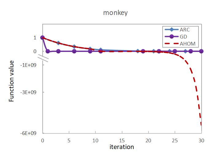
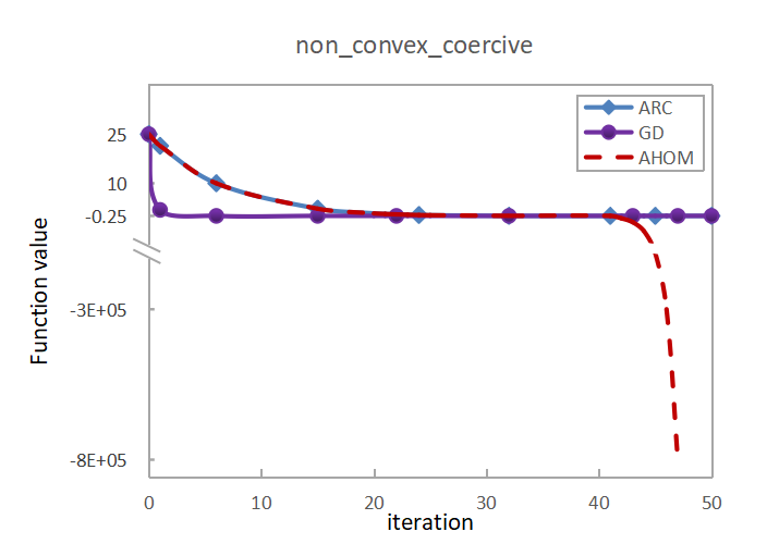
In fact, there are two degenerate saddle points and in these two problems respectively. As shown in Figure 1, the gradient descent method (GD) and the adaptive cubic regularization of Newton’s method (ARC) will get stuck at these two saddle points after a few iterations by selecting and as the initial points for the two problems respectively. To escape the degenerate saddle points, the notation of higher-order critical point was proposed in [1, 12] and the corresponding optimization algorithms were designed as well to find such higher-order critical points. By implementing these ideas to solve the monkey problem and the nonconvex coercive function, we find out in Figure 1 that by starting at the same initial points, the adaptive high order method (AHOM), which will be presented later in this paper, could indeed escape the aforementioned two degenerate saddle points, demonstrating the capability of high-order method for nonconvex optimization.
Prior to our work, there are several papers [1, 12, 13, 14] concerning optimization methods for computing higher-order critical points. In particular, Anandkumar and Ge [1] proposed a third-order algorithm that utilizes third-order derivative information and converges to a third-order critical point, i.e., it is a second-order point and satisfies additionally the third-order condition (see (2.10) for its definition). Cartis et al. [12] presented a trust-region method with -th order derivative for convexly constrained problems and it computes an -approximate -th () order critical points within at most iterations. Later on, such iteration bound was improved to in [13, 14]. Despite those theoretical development, the corresponding numerical experiments are absent and the practical issue regarding the implementation of their algorithms remains to be addressed. Specifically, a nonconvex subproblem, which is NP-hard in general, needs to be globally solved in each iteration of the algorithms in [12, 13, 14]. While Anandkumar and Ge’s [1] method assumes the knowledge of problem parameters such as the Lipschitz constants of the second-order and the third-order derivatives, which is hard to estimate in practice. As a matter of fact, an algorithm that does not depend on problem parameters is often desirable in optimization. Therefore, various adaptive strategies [5, 9, 10, 13, 14, 15, 17, 25, 3, 37, 27] have been adopted to adjust the parameters in the process of iteration. In this paper, we propose an adaptive high order method (AHOM) for problem (1.1), which incorporates Anandkumar and Ge’s approach [1] by some adaptive strategies. In particular, the adaptation on high-order regularization term is due to the single iteration of adaptive regularized -th order method (ARp) [5, 11] in each step of AHOM. While the dynamic estimation on the third-order Lipschitz constant is achieved by introducing a new successful criterion of the third-order critical measure. It turns out our AHOM is able to solve some nonconvex machine learning problems and escape the degenerate saddle points (see Section 5 for details).
Another merit of introducing high-order derivative information to optimization algorithms is the associated iteration complexity bounds could be improved. There are a few recent papers [2, 32, 33, 22, 21, 18, 26, 6] indicate that high-order derivatives indeed accelerate classical algorithms in the context of convex optimization. Similar phenomenon was also observed in the nonconvex optimization. For the unconstrained case, Nesterov [34] showed that the cubic regularization of Newton method can find an -approximate first-order critical point with at most evaluations of the objective function (and its derivatives), in contrast with the evaluation complexity of in the first-order method [31]. By using up to -th order derivatives, Birgin et al. [5] first proposed ARp method, whose evaluation complexity of finding first-order critical points is improved to . Later on, Cartis et al. [11] managed to adapt ARp method such that it is able to reach second-order critical points. In the mean while, the high-order method was also extended to accommodate constrained nonconvex optimization [13, 28, 4] and non-Lipschitz nonconvex optimization [14, 15]. Since our AHOM algorithm also belongs to the category of high-order method, we show that its iteration bound improves that of the algorithm in [1]. It worths mentioning that as we perform adaptations on both the high-order regularization term and estimator of the third-order Lipschitz constant, the corresponding iteration analysis becomes more technically involved than that in [1].
The rest of the paper is organized as follows. In Section 2, we introduce some preliminaries and the assumptions used throughout this paper. In Section 3, we propose our adaptive high order method (AHOM) for problem (1.1). Section 4 is devoted to analyzing the iteration bound of AHOM. In Section 5, we present some preliminary numerical results on solving -regularized nonconvex logistic regression problems, where AHOM is able to escape degenerate saddle point and even occasionally converges to a point satisfying second-order sufficient condition.
2 Preliminaries
In this section, we introduce notations, various approximate critical measures and present some basic assumptions that will be used in the paper.
2.1 Notations
Recall that a high-order tensor is a multidimensional array. In particular first-order and second-order tensors are vectors and matrices respectively. Throughout, we use the lower-case letters to denote vectors (e.g. ), the capital letters to denote matrices (e.g. ), and the capital calligraphy letters to denote high-order tensors (e.g. ), with subscripts of indices being their entries (e.g. ). For a -times differentiable function , the associated -th order derivative tensor is given by
| (2.2) |
where denotes .
The operations between tensor and vectors yields a multi-linear form
We say a tensor is symmetric if for any permutation of the indices . When is a symmetric tensor, we may make identical to the same vector in the above multi-linear form yielding that
Similarly, the multi-linear form with respect to matrices is defined as
where itself is a -th order tensor with being the dimension of -th direction. Suppose is the projection matrix associated with subspace . We call
| (2.3) |
is the projection tensor of on subspace . That is, any vectors applied to the projection tensor is equivalent to the projections of on applied to the original tensor:
The Frobenius norm of a -th order tensor is: , and the spectral norm of a -th order tensor is defined as
| (2.4) |
For a symmetric tensor , the spectral norm in (2.4) is equivalent to . In particular, the spectral norm of a symmetric matrix is equivalent to , where denotes the -th largest eigenvalue of . Note that all the matrices considered in this paper are symmetric.
2.2 Lipschitz Continuous Assumption
We assume that the -th order derivative (2.2) is globally Lipschitz continuous, i.e., there exits such that
| (2.5) |
where the is the tensor spectral norm of -th order tensor given by (2.4). In the rest of the paper we let .
With tensor notations, the Taylor expansion of function at can be written as:
| (2.6) |
When , there is a bound between and its Taylor expansion (Lemma 3 in [1]):
| (2.7) |
2.3 Approximate Critical Points
We define the first-order and second-order critical measures of problem (1.1) as
| (2.8) |
and
| (2.9) |
respectively, where is the smallest eigenvalue of Hessian matrix . Then, a point satisfying is an -approximate first-order critical point, and we call it an -approximate second-order critical point if it further satisfies .
Recall it was demonstrated in [1] that is a third-order critical point if it is a second-order critical point and
| (2.10) |
Following the idea in [1], we consider the eigen-subspace of the Hessian matrix below.
Definition 2.1.
For any symmetric matrix with a eigen-decomposition , we adopt to denote the span of eigenvectors with eigenvalue at most . That is
Now we are able to define the third-order critical measure of the objective function.
Definition 2.2 (-competitive subspace and third-order critical measure).
Given any and , let -competitive subspace at point be the largest eigen-subspace such that , where
| (2.11) |
is the norm of the third-order derivatives projected in this subspace. We call is the third-order critical measure of .
Note that our notation above is slightly different from that proposed by Anandkumar and Ge [1], where the adaptive estimator is fixed as . In contrast, we consider the -competitive subspace and third-order critical measure to exclude the dependence on the the third-order Lipschitz parameter . In fact, the reason to let as a third-order critical measure is that condition (2.10) is implied by . To see this, suppose . We observe that
according to definition 2.1. Then, for any , we have . That is , where is the projection matrix associated with the subspace . Combining this fact with , we conclude that for any
which is exactly the condition (2.10).
Therefore, we define the -approximate critical point as follows.
Definition 2.3.
We call an -approximate critical point of problem (1.1) if it satisfies
We end this section by presenting an algorithm named ACCS that can find a -competitive subspace efficiently.
Algorithm 1 ACCS (Algorithm for computing the -competitive subspace)
3 Adaptive High Order Method (AHOM)
This section aims to design an adaptive high order method (AHOM) that can find a third-order critical point.
3.1 The Single Iteration of Adaptive Regularized -th Order Method (SARp)
Before introducing the AHOM algorithm, we first present a subroutine in Algorithm 3.1 that will be invoked in every iteration of AHOM. In particular, we call this subroutine SARp algorithm, which is just a single iteration of adaptive regularized -th order method (ARp) in [11], and requires an approximate minimization of
where is adaptive coefficient of the -th order regularization term.
Algorithm 2 Single iteration of ARp (SARp)
We remark that the conditions in Step 1 of SARp are easily achievable by applying some existing algorithms like ARC method [9, 10]. As SARp is a single step of ARp, many useful properties of ARp can be carried over to SARp, which are summarized in the following lemma.
Lemma 3.1 ([11], Lemma 3.1, Lemma 3.3, Lemma 3.4).
Given , the mechanism of SARp guarantees the following properties of the approximate minimizer of .
-
(i)
,
-
(ii)
,
-
(iii)
.
With the lemma above, we are able to prove some bounds for the critical measures and the sufficient decrease on the objective function in terms of the distance between and .
Proposition 3.1.
Suppose that , then for all successful SARp (), there have
-
(i)
-
(ii)
-
(iii)
where and are defined in SARp algorithm.
3.2 The AHOM Algorithm
Now we are ready to present our AHOM algorithm in Algorithm 3.2.
Algorithm 3 Adaptive High Order Method (AHOM)
| (3.12) |
AHOM algorithm utilizes the first-order, second-order and third-order derivatives to make progress, and it stops when all the three critical measures are sufficiently small, i.e., , for some given with . The decrease of the first two order critical measures is achieved by iteratively performing SARp in Step . When the third-order critical measure on the trial point is large, a descent direction will be constructed. Then a nontrivial update will be performed if the sufficient relative decrease on the objective (i.e., ) further occurs. On the other hand, a step resulting in an insufficient relative decrease will be rejected by the algorithm, in the meanwhile the adaptive estimator will be increased by a factor of . It is also possible that the third-order critical measure is already below the given tolerance but either or is still large. In this case, Step will be skipped and . Furthermore, if is obtained by an unsuccessful SARp, actually equals to (that is is not updated). However, the cubic regularizer is updated in this case, which will lead to a possible update on the next trial point . Finally, we would like to mention that algorithm ATN in Step was proposed in [1] and is convergent by at most iterations in expectation (Theorem 7 in [1]). We present the details of ATN in the appendix for the reference of interested readers.
4 Iteration Complexity Analysis of AHOM
To provide the iteration bound for AHOM, like in [5, 11] we first want to define some ”successful” iterations. Since there are two regularization parameters: and , whether they are updated successfully defines two types of ”successful” iterations accordingly. We first consider the cubic regularizer in SARp.
Definition 4.1.
We say an iteration in AHOM is ”successful SARp” if the SARp called in Step of this iteration is successful (i.e., ), otherwise it is an ”unsuccessful SARp” iteration. Suppose is the total number of iterations in AHOM, we denote by
the index set of all iterations such that the associated trial point is successful in SARp, and the complementary set including all the ”unsuccessful SARp” iterations is denoted as
Recall that in Lemma 3.5 of [11], the total number of iterations in the ARp for second-order critical points can be bounded by a function of the number of successful SARp (i.e., ). At first glance, we don’t expect such bound holds true for AHOM as the iterate could possibly be updated at Step 2 of AHOM after preforming SARp, resulting a whole different sequence in contrast with that of ARp. However, we note that the universal bound in Lemma 3.2 of [11] for the cubic regularizer is still valid for in SARp. Therefore, the same relationship between the two iteration numbers in Lemma 3.5 of [11] is carried over to AHOM by a similar proof.
Lemma 4.1.
The mechanism of AHOM and its subroutine SARp guarantees that
| (4.13) |
where .
Next we consider the successful iteration defined by the update of .
Definition 4.2.
If an iteration in AHOM performs a nontrivial update in Step 2, we call it an ”third-order successful” iteration. Suppose is the total number of iterations in AHOM, we denote by
the index set of all ”third-order successful” iterations. While all the ”third-order unsuccessful” iterations are categorized into two sets:
and
respectively, due to the violation on the relative decrease or the third-order critical measure .
According to Lemma 4.1, it suffices to bound to establish the overall iteration complexity of AHOM. From Definition 4.1 and 4.2, we have the following identity:
Consequently,
| (4.14) | ||||
Next, we shall first bound the term: . Before doing so, we first provide the benefit of using the third-order information.
Lemma 4.2.
For iteration k of AHOM, suppose , , is a unit vector in such that . Let , then we have
| (4.15) |
i.e., iteration k is third-order successful.
Proof.
Let , and , then by using (2.7) we have that
From the assumption , one has that
Furthermore the construction of the competitive subspace implies that and thus
Therefore, combining the above inequalities with the assumption , which is equivalent to , yields that
which amounts to
meaning that the iteration k is a third-order successful iteration. ∎
Then it is easy to see that has an upper bound as shown below.
Lemma 4.3.
For all iteration in AHOM, we have that
| (4.16) |
where and .
Proof.
We note that is increased by a factor of only when and . However, we have shown in Lemma 4.2 that as long as and . Therefore, will not be updated once it exceeds . We introduce the factor in to accommodate case when is only slightly less than in its last update. ∎
As a consequence, we are able to bound the number of type unsuccessful iterations in AHOM.
Lemma 4.4.
It holds that
| (4.17) |
Proof.
The updating rule of in AHOM gives that
Thus we deduce inductively that
Therefore the conclusion follows by dividing by and then taking on both sides. ∎
With all the above results, we are now in position to state our main complexity result below.
Theorem 4.1.
Proof.
According to Lemma 4.1 and inequality (4.14), it suffices to bound the three terms: , and respectively. The upper bound of can be found in Lemma 4.4. To bound the other two terms, we note that the algorithm AHOM continues is due to either the first-order, the second-order or the third-order critical measure is still above the given tolerance, namely,
| (4.19) |
In the following, we shall bound , and under the above three scenarios.
We first bound the term . Suppose the current iteration , from (iii) in Proposition 3.1 and Proposition 4.2, we know that
| (4.20) |
Next, we further bound the inequality (4.20) from below according to the three scenarios in (4.19).
- 1.
- 2.
- 3.
Therefore, for any iteration , combining (4.21), (4.22) and (4.23) guarantees that:
Recalling is a universal lower bound of , one has that
| (4.24) | ||||
and concludes the desired upper bound
| (4.25) |
Then, we bound the number of . Suppose the current iteration , from (iii) in Proposition 3.1 and the mechanism of AHOM , we know that
| (4.26) |
and
| (4.27) |
Similarly, we further bound the inequality (4.26) from below according to the three scenarios in (4.19). The same argument for (4.21) and (4.22) implies that they are still valid for under scenario (a) and (b) in (4.19) respectively. In case of third condition (c) in (4.19) holds, we deduce from (4.26), (4.27) and part (i) in Proposition 3.1 have that
| (4.28) | ||||
where . Therefore, for any iteration , combining (4.21), (4.22), (4.28) and the argument for (4.25), we have the following desired bound:
| (4.29) |
Therefore, combining inequalities (4.14), (4.17), (4.25) and (4.29) altogether, one has that
Finally, by invoking Lemma 4.1, the total number of iterations can be upper bounded by
where is defined in (4.18). ∎
5 Numerical Experiments
In this section, we show the performance of our algorithm for solving the following nonconvex logistic regression problem:
| (5.30) |
where is a collection of data samples with labeled as or , and the regularization parameter . In contrast with the standard logistic regression, the loss in (5.30) is quantified as the square of the difference between the logistic function and the observed outcome , which thus is a nonconvex function. In fact, there has been some similar nonconvex loss function proposed and studied in [19, 29]. It worths mentioning that both the loss functions in (5.30) and [19, 29] belong to a broader function class named sigmoid function, and there is an optimization model tailored for sigmoid function called sigmoidal programming in [36].
Our experiments are conducted on 6 datasets all come from LIBSVM available at
https://www.csie.ntu.edu.tw/~cjlin/libsvmtools/datasets/binary.html. The summary of those datasets are shown in Table 1.
| Dataset | Number of Samples | Dimension |
|---|---|---|
| a1a | 1,605 | 123 |
| phishing | 11,055 | 68 |
| sonar | 208 | 60 |
| splice | 1,000 | 60 |
| svmguide1 | 3,089 | 4 |
| svmguide3 | 1,243 | 22 |
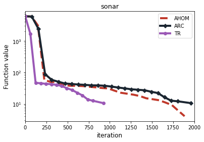
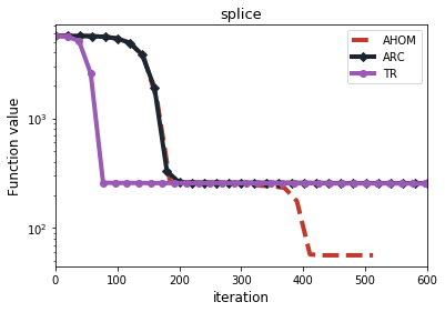
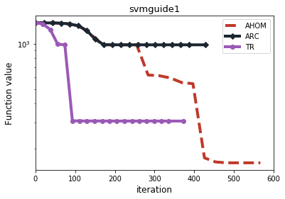
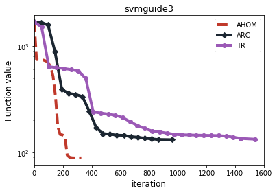
We apply AHOM algorithm with in the experiments and the subroutine SARp in each iteration reduces to the adaptive cubic regularization of Newton’s method (ARC). The parameters for the subroutine SARp are set as , which are the same as that of the benchmark algorithm: the adaptive cubic regularized Newton’s method (ARC). For the parameters in the main procedure of AHOM, we set , and . Particularly, we apply the so-called Lanczos [9] process to approximately solve the subproblem in SARp.
We compare our AHOM method (p=3) with two second order methods including: ARC and the trust region method (TR). We adopt the implementation of ARC and TR in the public package1 with the default parameters except that the full batch rather than the subsampled batch of the component functions is taken. In ARC, the “initial_penalty_parameter” and the “penalty_decrease_multiplier” (all parameters are same as those in SARp), the initial radius and the max radius of trust region in TR is and respectively. ††1 https://github.com/dalab/subsampled cubic regularization.
Recall that the first-order, second-order and third-order critical measures are given by , , respectively. We set equal error tolerances of for these three measures. Then an approximate third-order critical point satisfies (i) , (ii) , (iii), which is also the stopping criterion for AHOM. In addition, ARC and TR stops when (i) and (ii) are satisfied.
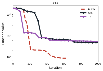
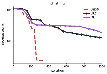
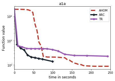
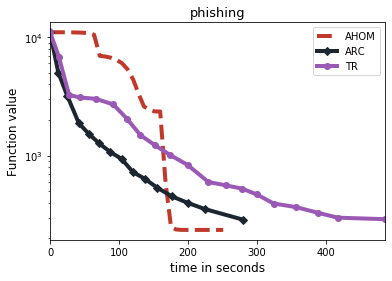
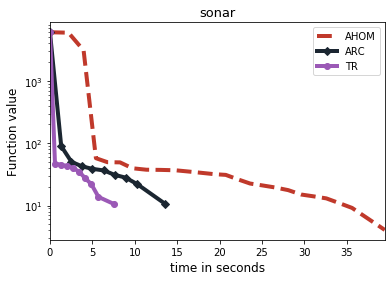
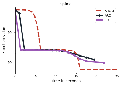
We plot figures to visualize the performance of AHOM and the two benchmark methods for solving problem (5.30). In particular, function value versus iterations and function values versus time of the three algorithms are shown in Figure 2 and Figure 3 respectively. We can see that AHOM is able to converge to a better solution for all the six datasets, while the other two methods may get stuck at some lower-order critical point. This indicates that using third-order information can really help to escape some degenerate saddle points. The detailed information about function value and the three critical measures of the output points of the three algorithms is presented in Table 2, where we can see that AHOM even occasionally converges to a point satisfying second-order sufficient condition (see the rows for the dataset “splice” and “svmguide1”).
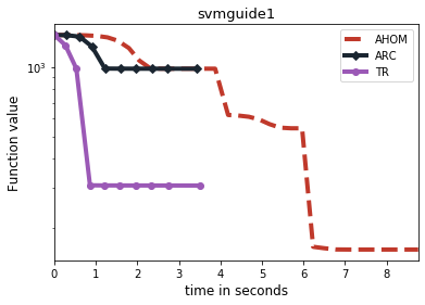
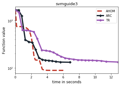
| Algorithm | ||||
|---|---|---|---|---|
| a1a | ||||
| AHOM | 87.6710 | 1.8122e-10 | 1e-05 | 1.6990e-13 |
| ARC | 138.1366 | 4.8090e-07 | 1e-05 | – |
| TR | 227.2495 | 3.8878e-07 | 4.8523e-06 | – |
| phishing | ||||
| AHOM | 236.1797 | 5.5960e-08 | 1e-05 | 0 |
| ARC | 287.9241 | 9.4991e-07 | 8.5778e-06 | – |
| TR | 291.0511 | 6.1220e-07 | 1e-05 | – |
| sonar | ||||
| AHOM | 4.0587 | 4.1230e-07 | 9.3519e-06 | 2.5533e-15 |
| ARC | 10.5456 | 4.9407e-07 | 9.8599e-06 | – |
| TR | 10.5456 | 7.1172e-08 | 9.8573e-06 | – |
| splice | ||||
| AHOM | 56.2595 | 3.4501e-13 | 0.3029 | 0 |
| ARC | 116.7087 | 7.6571e-07 | 6.7674e-05 | – |
| TR | 95.6435 | 2.0769e-07 | 7.0064e-05 | – |
| svmguide1 | ||||
| AHOM | 161.2606 | 8.6737e-10 | 4.0163 | 0 |
| ARC | 982.5015 | 7.2893e-07 | 4.4215e-05 | – |
| TR | 305.6594 | 2.9699e-08 | 3.7649e-05 | – |
| svmguide3 | ||||
| AHOM | 89.1117 | 7.7390e-07 | 1e-05 | 0 |
| ARC | 131.9918 | 8.1708e-07 | 1e-05 | – |
| TR | 133.4102 | 8.0748e-07 | 1e-05 | – |
Acknowledgments
We would like to thank Professor Qi Deng at Shanghai University of Finance and Ecomoics for the discussion on the numerical experiment of this paper.
References
- Anandkumar and Ge, [2016] Anandkumar, A. and Ge, R. (2016). Efficient approaches for escaping higher order saddle points in non-convex optimization. In Conference on Learning Theory, pages 81–102.
- Baes, [2009] Baes, M. (2009). Estimate sequence methods: extensions and approximations. Institute for Operations Research, ETH, Z rich, Switzerland.
- Bellavia et al., [2019] Bellavia, S., Gurioli, G., Morini, B., and Toint, P. L. (2019). Adaptive regularization algorithms with inexact evaluations for nonconvex optimization. SIAM Journal on Optimization, 29(4):2881–2915.
- Birgin et al., [2016] Birgin, E. G., Gardenghi, J., Martínez, J. M., Santos, S. A., and Toint, P. L. (2016). Evaluation complexity for nonlinear constrained optimization using unscaled KKT conditions and high-order models. SIAM Journal on Optimization, 26(2):951–967.
- Birgin et al., [2017] Birgin, E. G., Gardenghi, J., Martínez, J. M., Santos, S. A., and Toint, P. L. (2017). Worst-case evaluation complexity for unconstrained nonlinear optimization using high-order regularized models. Mathematical Programming, 163(1-2):359–368.
- Bubeck et al., [2018] Bubeck, S., Jiang, Q., Lee, Y. T., Li, Y., and Sidford, A. (2018). Near-optimal method for highly smooth convex optimization. arXiv preprint arXiv:1812.08026.
- Carmon et al., [2017] Carmon, Y., Duchi, J. C., Hinder, O., and Sidford, A. (2017). Lower bounds for finding stationary points I. Mathematical Programming, pages 1–50.
- Carmon et al., [2018] Carmon, Y., Duchi, J. C., Hinder, O., and Sidford, A. (2018). Accelerated methods for nonconvex optimization. SIAM Journal on Optimization, 28(2):1751–1772.
- [9] Cartis, C., Gould, N. I., and Toint, P. L. (2011a). Adaptive cubic regularisation methods for unconstrained optimization. part I: motivation, convergence and numerical results. Mathematical Programming, 127(2):245–295.
- [10] Cartis, C., Gould, N. I., and Toint, P. L. (2011b). Adaptive cubic regularisation methods for unconstrained optimization. part II: worst-case function-and derivative-evaluation complexity. Mathematical programming, 130(2):295–319.
- Cartis et al., [2017] Cartis, C., Gould, N. I., and Toint, P. L. (2017). Improved second-order evaluation complexity for unconstrained nonlinear optimization using high-order regularized models. arXiv preprint arXiv:1708.04044.
- Cartis et al., [2018] Cartis, C., Gould, N. I., and Toint, P. L. (2018). Second-order optimality and beyond: Characterization and evaluation complexity in convexly constrained nonlinear optimization. Foundations of Computational Mathematics, 18(5):1073–1107.
- Cartis et al., [2020] Cartis, C., Gould, N. I., and Toint, P. L. (2020). Sharp worst-case evaluation complexity bounds for arbitrary-order nonconvex optimization with inexpensive constraints. SIAM Journal on Optimization, 30(1):513–541.
- Chen and Toint, [2020] Chen, X. and Toint, P. L. (2020). High-order evaluation complexity for convexly-constrained optimization with Non-Lipschitzian group sparsity terms. Mathematical Programming, to appear.
- Chen et al., [2019] Chen, X., Toint, P. L., and Wang, H. (2019). Complexity of partially separable convexly constrained optimization with Non-Lipschitzian singularities. SIAM Journal on Optimization, 29(1):874–903.
- Curtis et al., [2018] Curtis, F. E., Robinson, D. P., and Samadi, M. (2018). An inexact regularized Newton framework with a worst-case iteration complexity of for nonconvex optimization. IMA Journal of Numerical Analysis, 39(3):1296–1327.
- Duchi et al., [2011] Duchi, J., Hazan, E., and Singer, Y. (2011). Adaptive subgradient methods for online learning and stochastic optimization. Journal of Machine Learning Research, 12(Jul):2121–2159.
- Gasnikov et al., [2018] Gasnikov, A., Kovalev, D., Mohhamed, A., and Chernousova, E. (2018). The global rate of convergence for optimal tensor methods in smooth convex optimization. arXiv preprint arXiv:1809.00382.
- Ghadimi et al., [2019] Ghadimi, S., Lan, G., and Zhang, H. (2019). Generalized uniformly optimal methods for nonlinear programming. Journal of Scientific Computing, 79(3):1854–1881.
- Gould et al., [2019] Gould, N. I., Rees, T., and Scott, J. A. (2019). Convergence and evaluation-complexity analysis of a regularized tensor-Newton method for solving nonlinear least-squares problems. Computational Optimization and Applications, 73(1):1–35.
- [21] Grapiglia, G. and Nesterov, Y. (2019a). Tensor methods for finding approximate stationary points of convex functions. arXiv preprint arXiv:1907.07053.
- [22] Grapiglia, G. and Nesterov, Y. (2019b). Tensor methods for minimizing functions with hölder continuous higher-order derivatives. arXiv preprint arXiv:1904.12559.
- Gratton et al., [2019] Gratton, S., Simon, E., and Toint, P. L. (2019). Minimization of nonsmooth nonconvex functions using inexact evaluations and its worst-case complexity. arXiv preprint arXiv:1902.10406.
- Jiang et al., [2019] Jiang, B., Lin, T., Ma, S., and Zhang, S. (2019). Structured nonconvex and nonsmooth optimization: Algorithms and iteration complexity analysis. Computational Optimization and Applications, 72:115–157.
- [25] Jiang, B., Lin, T., and Zhang, S. (2020a). A unified adaptive tensor approximation scheme to accelerate composite convex optimization. SIAM Journal on Optimization, to appear.
- [26] Jiang, B., Wang, H., and Zhang, S. (2020b). An optimal high-order tensor method for convex optimization. Mathematics of Operations Research, to appear.
- Lucchi and Kohler, [2019] Lucchi, A. and Kohler, J. (2019). A stochastic tensor method for non-convex optimization. arXiv preprint arXiv:1911.10367.
- Martínez, [2017] Martínez, J. M. (2017). On high-order model regularization for constrained optimization. SIAM Journal on Optimization, 27(4):2447–2458.
- Mason et al., [1999] Mason, L., Baxter, J., Bartlett, P., and Frean, M. (1999). Boosting algorithms as gradient descent infunction space. In Advances in neural information processing systems, pages 512–518.
- Murty and Kabadi, [1987] Murty, K. and Kabadi, S. (1987). Some np-complete problems in quadratic and nonlinear programming. Mathematical Programming, 39:117–129.
- Nesterov, [2004] Nesterov, Y. (2004). Introductory lectures on convex optimization a basic course. Applied Optimization, 87(5):xviii,236.
- Nesterov, [2008] Nesterov, Y. (2008). Accelerating the cubic regularization of Newton’s method on convex problems. Mathematical Programming, 112(1):159–181.
- Nesterov, [2019] Nesterov, Y. (2019). Implementable tensor methods in unconstrained convex optimization. Mathematical Programming, published onlone:doi:10.1007/s10107–019–01449–1.
- Nesterov and Polyak, [2006] Nesterov, Y. and Polyak, B. T. (2006). Cubic regularization of Newton method and its global performance. Mathematical Programming, 108(1):177–205.
- Nie, [2015] Nie, J. (2015). The hierarchy of local minimums in polynomial optimization. Mathematical Programming, 151(2):555–583.
- Udell and Boyd, [2013] Udell, M. and Boyd, S. (2013). Maximizing a sum of sigmoids. Optimization and Engineering, pages 1–25.
- Zheng and Zheng, [2019] Zheng, Y. and Zheng, B. (2019). A modified adaptive cubic regularization method for large-scale unconstrained optimization problem. arXiv preprint arXiv:1904.07440.
Appendix A A Algorithm for Approx Tensor Norm
The details of algorithm ATN in Step of AHOM are shown as follows.
Algorithm 4 Approximate Tensor Norms (ATN)
The above algorithm was proposed in [1] and it aims to find a vector such that the value is an approximation of . The following theorem reveals that this algorithm converges by at most iterations in expectation.
Theorem A.1 ([1] Theorem 7).
There is a universal constant B such that the expected number of iterations of Algorithm ATN is at most 2, and the output of ATN is a unit vector that satisfies for .