The disintegrating old open cluster Czernik 3

Abstract

We have performed a detailed analysis of the Czernik 3 (Cz3) open cluster by using deep near-infrared photometry taken with TIRCAM2 on 3.6m Devasthal optical telescope along with the recently available high quality proper motion data from the Gaia DR2 and deep photometric data from Pan-STARRS1. The cluster has a highly elongated morphology with fractal distribution of stars. The core and cluster radii of the cluster are estimated as 0.5 pc and 1.2 pc, respectively. We have identified 45 stars as cluster members using the Gaia proper motion data. The distance and age of the cluster are found to be $3.5\pm 0.9$ kpc and $0.9^{+0.3}_{-0.1}$ Gyr, respectively. The slope of the mass function $`\Gamma^{\prime}$ in the cluster region, in the mass range $\sim$0.95$<$M/M_⊙$<$2.2, is found to be $-1.01\pm 0.43$. The cluster shows the signatures of mass-segregation and is dynamically relaxed (dynamical age=10 Myr). This along with its small size, big tidal radius, low density/large separation of stars, and elongated and distorted morphology, indicate that the Cz3 is a loosely bound disintegrating cluster under the influence of external tidal interactions.

1 Introduction

Most of the stars form in a clustered environment in molecular clouds (Lada & Lada, 2003). The dynamics of stars in the clusters as well as the structure of clusters measured as a function of cluster age hold important clues on the processes of star formation and stellar evolution. The Galactic disk is abundant in stars, spiral arms, and giant molecular clouds. Therefore, star clusters located in the disk are subjected to disturbance, such as disk shock, spiral arm passage, molecular cloud encounters, etc. (Spitzer & Harm, 1958; Kruijssen, 2012). As clusters age, the expulsion of gas by stellar feedback as well as dynamical interactions between stars and binary systems in the cluster soften its gravitational potential, leading to their expansion and to their partial or total dissolution into the field of their host galaxy (e.g., Spitzer & Harm, 1958; Dib et al., 2011; Parker & Meyer, 2012; Dib et al., 2013; Parker & Dale, 2013; Pfalzner & Kaczmarek, 2013; Brinkmann et al., 2017; Dib et al., 2018). The typical survival timescale of open clusters in the Galactic disk is about 200 Myr (Bonatto et al., 2006; Yang et al., 2013). Open clusters much older than the survival timescale usually have distorted shape and loosened structure which leads to their disruption. The disintegrated open clusters will then become moving groups and supply field stars (Tang et al., 2019).

The core (nucleus) and the corona (extended region of the star cluster) are two main regions in open clusters (e.g., Kholopov, 1969; Pandey et al., 1990; Sharma et al., 2006). The nucleus of the cluster usually contains bright and massive stars along with few low-mass stars, whereas the corona, relatively contains a large number of faint low-mass stars (Brandl et al., 1999; Sharma et al., 2006, 2008). Whether this segregation of massive stars towards the central region of a cluster occurs due to an evolutionary effect or is of primordial origin is not yet entirely clear. In the first scenario, massive stars may form anywhere in the cluster and eventually sink to the cluster center through the effects of two-body relaxation (e.g., McMillan et al., 2007; Allison et al., 2009b). This is supported by numerical simulations in which mass segregation occurs on time-scales that are of the order of the cluster’s ages (e.g., Allison et al., 2010; Parker, 2014). The second scenario suggests that massive stars form preferentially in the central region of the cluster either by efficiently accreting gas due to their location at the bottom of the cluster potential well (Dib et al., 2010) or by a coalescence process of less massive stars (Dib, 2007; Dib et al., 2008). The time-scale for this mass-segregation to complete is still not very well known and is important to know its implication on the dissolution of star clusters. The second scenario is an active area of research, especially because of the need to understand trapezium-type sub-systems in star clusters (Mermilliod, 2000), and the associated implications for the formation mechanisms of massive stars (Bonnell et al., 1998).

During the past decade several studies on star clusters, stellar evolution and dynamics have been carried out. However, most of these studies are not always based on deep photometric data and lacks the membership determination based on high-quality proper motion (PM) data. Czernik 3 ($\alpha_{J2000}$: $01^{h}03^{m}06^{s}$, $\delta_{J2000}$: $+62^{\circ}47^{\prime}00^{\prime\prime}$ (Dias et al., 2002); hereafter Cz3, cf. Fig. 1), one of the poorly studied open clusters, is located in the Galactic plane towards the 2^nd Galactic quadrant ($l$ = 124^∘.265, $b$ = -0^∘.058). This cluster is cataloged in the OPENCLUST as well as in MWSC with the distance and age in the range 1.4 - 1.6 kpc and 100 - 630 Myr, respectively. Recently, Bisht et al. (2017) placed this cluster at a distance of 1.75 kpc with an age of 115 Myr, using the 2MASS data. Since most of the information about this cluster is derived from the not-so-deep photometric surveys, we have revisited this cluster and performed a detailed analysis to understand its dynamical evolution by using our deep near-infrared (NIR) observations taken from the recently installed 3.6m telescope at Devasthal, Nainital, India (Kumar et al., 2018), along with the recently available data from the Gaia data release 2 (Gaia Collaboration et al., 2016, 2018) and Pan-STARR1 (Chambers et al., 2016).

In this paper, Section 2 describes the observations and data reduction. The structure of this cluster, membership probability of stars in the cluster region, fundamental parameters (i.e., age and distance) of the cluster, and mass function (MF) analyses are presented in Section 3. The dynamical structure of this cluster is discussed in Section 4, and we conclude our studies in Section 5.

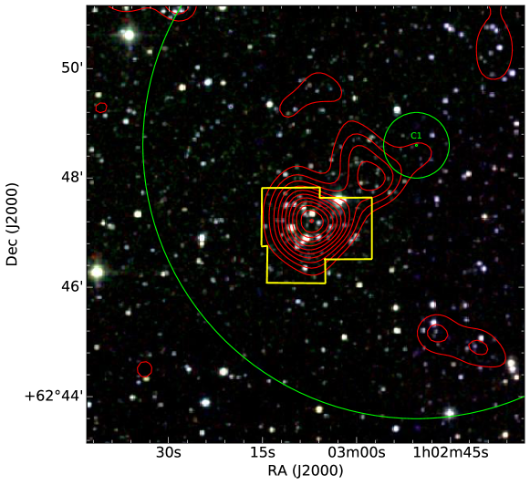
Figure 1: (Left panel): Color-composite image obtained using the $J$ (blue), $H$ (green), and $K$ (red) 2MASS images for an area of $\sim 10\times 10$ arcmin² around the Cz3 cluster. The yellow region encloses the present observations using TIRCAM2. The small and big green circles are the core and the cluster regions identified by Bisht et al. (2017). The red contours are the isodensity contours generated using nearest neighbor method from the 2MASS data (cf. Section 3.1). (Right panels): Comparison of the colour-composite images obtained by using the $J$ (blue), $H$ (green), and $K$ (red) images for the core region of the Cz3 cluster from the 2MASS (top panel) and TIRCAM2 observations (bottom panel).

2 Multi-wavelength data sets

2.1 Deep NIR data

Deep NIR $J$ (1.20 $\mu$m), $H$ (1.65 $\mu$m) and $K$ (2.19 $\mu$m) band photometric observations of the Cz3 open cluster (cf. Fig. 1) were taken during the night of 2017 October 7 using TIFR Near Infrared Imaging Camera-II (TIRCAM2; Naik et al., 2012; Baug et al., 2018) mounted at the Cassegrain main port of the 3.6m ARIES Devasthal Optical Telescope (DOT; Kumar et al., 2018). The weather conditions in these nights were good with relative humidity $<60$ percent and the full-width at half maxima of the stellar images was $\sim$0.6 arcsec. The field of view (FOV) of the TIRCAM2 is $\sim 86.5\times 86.5$ arcsec square with a plate scale of 0.169 arcsec. We took four pointings of the Cz3 open cluster covering the central cluster region ($\sim$3 arcmin square) and in each pointing several frames in a 5-point dither pattern were taken with exposure times of 50 sec, 50 sec, and 10 sec in $J,~{}H,$ and $K$ bands, respectively. The total exposure times were 500 sec, 500 sec and 1000 sec in each pointing in $J,~{}H,$ and $K$ bands, respectively. Dark and sky flats were also taken during the observations. Sky frames in each filter were generated from the median of the dithered frames.

The basic image processing such as dark/sky subtraction and flat fielding was done using tasks available within IRAF. Instrumental magnitudes were obtained using the DAOPHOT package. As the cluster region is crowded we carried out point spread function (PSF) photometry to get the magnitudes of the stars. Astrometry of the stars was done using the Graphical Astronomy and Image Analysis Tool with a rms noise of the order of $\sim$0.1 arcsec. The calibration of the photometry to the standard system was done using the following transformation equations:

$$(J-H)=(0.84\pm 0.13)\times(j-h)+(0.35\pm 0.03)$$ (1)

$$(J-K)=(0.77\pm 0.12)\times(j-k)+(1.11\pm 0.07)$$ (2)

$$(J-j)=(-0.12\pm 0.13)\times(J-H)-(4.06\pm 0.07)$$ (3)

where the capital $JHK$ are the standard magnitudes of the stars taken from the 2MASS catalog and the small $jhk$ are the present instrumental magnitudes of the similar stars normalized per sec exposure time. The typical DAOPHOT errors as a function of corresponding standard magnitudes are shown in Fig. 2. We have used only those stars for further analyses which are having signal-to-noise ratio greater than 10 (photometric errors $<$ 0.1 mag). In total, 133 stars were identified in the central region of the Cz3 cluster with detection limits of 19.9 mag, 18.6 mag, 18.2 mag in $J$, $H$, $K$ bands, respectively. Some of the brighter stars (18 in total) were saturated in our observations; we have taken their respective magnitudes from the 2MASS point source catalog. The positions and magnitudes of the stars in different bands are given in Table 1.

Figure 2: DAOPHOT errors as a function of $J,H,$ and $K$ magnitudes.

Table 1: Sample of the NIR photometry of the stars in the present study. The complete table is available in the electronic form only.

ID	$\alpha_{(2000)}$	$\delta_{(2000)}$	$J\pm\sigma~{}~{}~{}~{}~{}$	$H\pm\sigma~{}~{}~{}~{}~{}$	$K\pm\sigma~{}~{}~{}~{}~{}$
	$(degree)$	$(degree)$	(mag)	(mag)	(mag)
1	15.762209	+62.793190	$8.523\pm 0.021$	$7.937\pm 0.017$	$7.787\pm 0.018$
2	15.783788	+62.781624	$10.577\pm 0.024$	$9.600\pm 0.021$	$9.277\pm 0.020$
3	15.793315	+62.784641	$10.904\pm 0.021$	$10.092\pm 0.017$	$9.866\pm 0.019$
4	15.779851	+62.789120	$12.475\pm 0.025$	$11.515\pm 0.024$	$11.127\pm 0.022$
5	15.784626	+62.772507	$12.550\pm 0.021$	$12.047\pm 0.021$	$11.940\pm 0.023$

2.2 Archival data

In order to study a wider area around Cz3, we have selected a FOV of $10\times 10$ arcmin square as shown in Fig. 1 and downloaded the available data from the below mentioned archives:

2.2.1 Gaia

The second Gaia data release, Gaia DR2 (Gaia Collaboration et al., 2016, 2018), which consists of astrometry, photometry, radial velocities, and information on astrophysical parameters and variability for sources brighter than $G$ (0.33-1.05 $\micron$) = 21 magnitude. Gaia DR2 contains celestial positions and apparent brightness in $G$ band for approximately 1.7 billion sources. In addition, for 1.3 billion of those sources, parallaxes and PMs are available. This data release also contains the broad-band colour information in the form of the apparent brightness in the $G_{BP}$ (0.33-0.68 $\micron$) and $G_{RP}$ (0.63-1.05 $\micron$) bands for 1.4 billion sources. We have downloaded the Gaia DR2 data from the data archive. The $Gaia$ sample consists of stars with error in their PM values less than 3 mas yr^-1.

2.2.2 Pan-STARRS1

The Panoramic Survey Telescope and Rapid Response System (Pan-STARRS1 or PS1) imaged the entire northern sky, above a declination of $\delta\sim-30^{\circ}$, in five broadband filters $(g,r,i,z,y)_{P1}$, which encompass the spectral window from $\sim$0.4 - 1.05 $\micron$. The survey, which included multiple pointings per observed field per filter, reached a depth of $g_{P1}\sim 23.2$ mag, $r_{P1}\sim 23.2$ mag, and $i_{P1}\sim 23.1$ mag in the stacked images. The details about the PS1 surveys and latest data products are given in Chambers et al. (2016). We have downloaded images as well as point source catalog from the data release 2 of the PS1. While PS1 had observations at multiple epochs, however the analysis reported in the ensuing sections have used average magnitudes in each band. The PS1 sample consists of stars with photometric uncertainties less than 0.1 mag in different PS1 bands.

2.2.3 2MASS

We have also used the 2MASS point source catalog (Cutri et al., 2003) for NIR (JHK_s) photometry in the Cz3 region. This catalog is reported to be 99 percent complete down to the limiting magnitudes of 15.8 mag, 15.1 mag and 14.3 mag in the $J$ (1.24 $\mu$m), $H$ (1.66 $\mu$m) and $K_{s}$ (2.16 $\mu$m) band, respectively. The 2MASS sample consists of stars with photometric uncertainties less than 0.1 mag in the $J$, $H$ and $K_{s}$ bands.

3 Results and Analysis

3.1 Structure of the Cz3 cluster

To study the structure of the Cz3 open cluster, we obtained stellar number density maps for the sample of stars taken from the PS1, $Gaia$, and 2MASS surveys covering $10\times 10$ arcmin square FOV around this cluster region. We have also generated the stellar number density map for a sample of member stars of Cz3 cluster (cf. Section 3.2). The stellar number density maps were generated using the nearest neighbor (NN) method as described by Gutermuth et al. (2005). We took the radial distance necessary to encompass the sixth nearest stars and computed the local surface density in a grid size of 5 arcsec (cf. Gutermuth et al., 2009). The stellar number density contours derived by this method are plotted in Fig. 3 as black curves smoothened to a grid of size $3\times 3$ pixels. The lowest contour is 1$\sigma$ above the mean of stellar density and the step size is equal to the 1$\sigma$. As can be seen from the contours, the central core region of this cluster is almost circular, whereas the outer region is highly elongated and has another peak of lower density. To study the structure of the cluster, a reliable membership, e.g., on the basis of PM, is required. The PM errors in the Gaia data towards fainter magnitudes are very high, hence we used the PS1 data which has similar depth as Gaia data to demarcate the cluster extent and core region of the Cz3. The cluster extent (lowest density contour) and core (region within the half of the peak value of stellar density) are shown with red circle and red contour, respectively, in the panel (a) of Fig. 3. We have divided the cluster region into two parts, one containing the central region and other containing the extended region. The demarcation between these two regions is shown with a dotted line. The core region, centered at $\alpha_{J2000}$: $01^{h}03^{m}06^{s}.9$, $\delta_{J2000}$: $+62^{\circ}47^{\prime}00^{\prime\prime}$, has a radius of $\sim$30 arcsec. Bisht et al. (2017) have derived slightly off-center coordinates of this cluster as $\alpha_{J2000}$: $01^{h}02^{m}50^{s}.4$, $\delta_{J2000}$: $+62^{\circ}48^{\prime}36^{\prime\prime}$, with core and cluster radii as 36 arcsec and 300 arcsec, respectively (cf. Fig. 1).

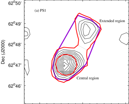
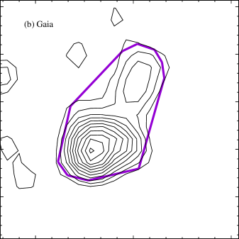
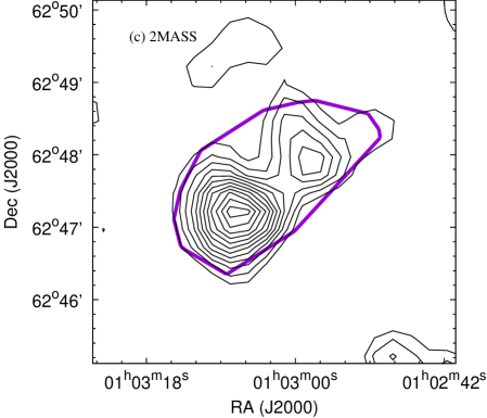
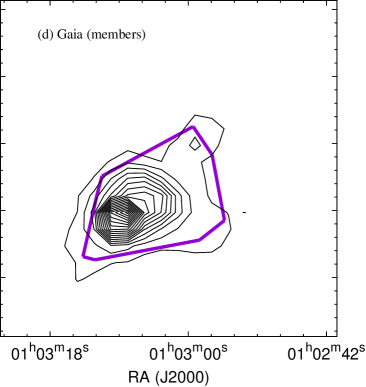
Figure 3: Stellar density contours (black curves) generated by using the nearest neighbor method from the PS1 (panel a), $Gaia$ (panels b and d), and 2MASS (panel c) data. Panel (d) represents isodensity contours derived by using the location of member stars (cf. Section 3.2). The purple curve represents the Qhull for the stars located within the lowest density contour. In panel (a), the red density contour and red circle represent the cluster and core regions, respectively. The dotted line represents the demarcation between the central and extended regions.

Table 2: Structural parameters of the CZ3 cluster.

ID	Sample	ntotal	$n_{hull}$	Ahull	Acluster	Rcluster	Rcirc	Aspect
				$(arcmin^{2})$	$(arcmin^{2})$	$(arcmin)$	$(arcmin)$	ratio
(a)	PS1	131	9	4.05	4.35	1.18	1.65	1.96
(b)	$Gaia$	176	10	4.16	4.40	1.18	1.61	1.86
(c)	2MASS	73	13	4.00	4.87	1.25	1.60	1.64
(d)	Gaia (members)	45	8	2.69	3.27	1.02	1.27	1.55
	Average	-	-	3.73	4.22	1.16	1.53	1.75

As the cluster is showing highly elongated morphology, we refine the definition of the cluster area using the convex hull rather than a circular area around the objects, as the later method tends to significantly overestimate the area of the cluster, in particular if the cluster is elongated or irregularly shaped rather than spherical (Schmeja & Klessen, 2006). The convex hull for the stars located within the lowest density contour is computed using the program Qhull. We estimate the area of the cluster $A_{cluster}$ using the convex hull of the data points, normalized by an additional geometrical factor taking into account the ratio of the number of objects inside and on the convex hull (Hoffman et al., 1983; Schmeja & Klessen, 2006):

$$A_{cluster}={{A_{hull}}\over{(1-{n_{hull}\over n_{total}})}}$$ (4)

where, $A_{hull}$ is the area of convex hull, $n_{hull}$ is the number of vertices on convex hull, and $n_{total}$ is the number of objects. The correction factor is used since the convex hull by itself tends to be smaller than the true sampling window. To be consistent, we define the cluster radius $R_{cluster}$ as the radius of a circle with the same area $A_{cluster}$. We have also estimated the circular radial size, $R_{circ}$, defined as half of the largest distance between any two members, the radius of the minimum area circle that encloses the entire grouping. For each data sets, the estimated values for $A_{hull}$, $A_{cluster}$, $R_{cluster}$ and $R_{circ}$ are listed in Table 2. The ratio $R^{2}_{circ}\over{R^{2}_{cluster}}$, which is a measure of the aspect ratio of a cluster (Gutermuth et al., 2009) is also listed in the same table. In general, these values suggest towards a highly elongated morphology of this cluster. The estimated extent of the cluster ($R_{cluster}$ =1.18 arcmin from PS1 sample) is much smaller than the values reported in the previous studies.

3.2 Membership Probability

Gaia DR2 release has opened up the possibility of an entirely new perspective on the problem of membership determination in cluster studies by providing the new and precise parallax measurements upto very faint limits. To determine the membership probability, we adopted the method described in Balaguer-Núnez et al. (1998). This method has previously been used extensively (see e.g., Bellini et al. (2009, $\omega$ Centauri); Sariya et al. (2012, NGC 6809); Yadav et al. (2013, NGC 3766); Sariya et al. (2017, NGC 3201)). In this method, we first construct the frequency distributions of cluster stars ($\phi^{\nu}_{c}$) and field stars ($\phi^{\nu}_{f}$) using the following equations:

$$\centering\tiny\begin{split}\phi^{\nu}_{c}={1\over{2\pi\sqrt{(\sigma^{2}_{c}+\epsilon^{2}_{xi})(\sigma^{2}_{c}+\epsilon^{2}_{yi})}}}\\ \times{\exp\left\{{-{1\over 2}\left[\,{{{(\mu_{xi}-\mu_{xc})^{2}}\over{\sigma^{2}_{c}+\epsilon^{2}_{xi}}}+{{(\mu_{yi}-\mu_{yc})^{2}}\over{\sigma^{2}_{c}+\epsilon^{2}_{yi}}}}\right]\,}\right\}}\end{split}\@add@centering$$ (5)

$$\centering\tiny\begin{split}\phi^{\nu}_{f}={1\over{2\pi\sqrt{1-\gamma^{2}}\sqrt{(\sigma^{2}_{xf}+\epsilon^{2}_{xi})(\sigma^{2}_{yf}+\epsilon^{2}_{yi})}}}\\ \times{\exp\left\{{-{1\over{2(1-\gamma^{2})}}\left[\,{{{(\mu_{xi}-\mu_{xf})^{2}}\over{\sigma^{2}_{xf}+\epsilon^{2}_{xi}}}-{{2\gamma(\mu_{xi}-\mu_{xf})(\mu_{yi}-\mu_{yf})}\over{\sqrt{(\sigma^{2}_{xf}+\epsilon^{2}_{xi})(\sigma^{2}_{yf}+\epsilon^{2}_{yi})}}}+{{(\mu_{yi}-\mu_{yf})^{2}}\over{\sigma^{2}_{yf}+\epsilon^{2}_{yi}}}}\right]\,}\right\}}\end{split}\@add@centering$$ (6)

where $\mu_{xi}$, $\mu_{yi}$ and $\epsilon_{xi},\epsilon_{yi}$ are the PMs and the errors in PMs of the $i^{th}$ star, respectively. $\mu_{xc}$, $\mu_{yc}$ and $\sigma_{c}$, and $\mu_{xf}$, $\mu_{yf}$ and $\sigma_{xf}$, $\sigma_{yf}$ are the PM center and the PM dispersion of the cluster and field stars, respectively. Subscript ‘x’ refers to the RA component of the PM corrected with geometric transformation, whereas subscript ‘y’ refers to the Dec component of the PM. $\gamma$ is the correlation coefficient which is calculated as:

$$\gamma={{(\mu_{xi}-\mu_{xf})(\mu_{yi}-\mu_{yf})}\over{\sigma_{xf}\sigma_{yf}}}$$ (7)

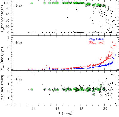
Figure 4: Panel 1 & 2: PM vector-point diagrams (panel 1) and Gaia DR2 $G$ vs. $(G_{BP}-G_{RP})$ CMDs (panel 2) for stars located in the Cz3 cluster region. The left sub-panels (1(a) and 2(a)) show all stars, while the middle (1(b) and 2(b)) and the right sub-panels (1(c) and 2(c)) show the probable cluster members and field stars, respectively. Panel 3: Membership probability P_μ, PM errors $\sigma_{PM}$ and parallax of stars as a function of $G$ magnitude for stars in the Cz3 cluster region. Forty five stars with P${}_{\mu}>$90 percent are considered as member of the Cz3 cluster and are shown by green circles with black rings.

Gaia PM data located within the convex hull of the cluster region are used here to determine membership probability of cluster member stars. PMs $\mu_{x}$ and $\mu_{y}$ are plotted as vector-point diagrams (VPDs) in the panel 1 of Fig. 4. The panel 2 shows the corresponding $G$ versus $G_{BP}-G_{RP}$ colour-magnitude diagrams (CMDs). The dots in sub-panel 1(a) represent PM distribution of all the stars where a prominent clump within a radius of $\sim$0.6 mas yr^-1 centered at $\mu_{xc}$ = -0.23 mas yr^-1, $\mu_{yc}$ = -0.31 mas yr^-1 can bee seen. This population of stars have almost similar PMs and have high probability for cluster membership. Remaining stars with scattered PM values are most probably a field population. This is more clearer in the VPDs and CMDs of probable cluster and field populations as shown in the sub-panels 1(b), 1(c), 2(b), and 2(c), respectively. The probable cluster members are showing well defined MS in the CMD which is usually seen for the similar population of stars. On the other hand, the probable field stars are quite obvious by their broad distribution in the CMD. Assuming a distance of 3.5 kpc (the present estimate for the Cz3 cluster, Section 3.3) and a radial velocity dispersion of 1 km s^-1 for open clusters (Girard et al., 1989), the expected dispersion ($\sigma_{c}$) in PMs would be $\sim$0.06 mas yr^-1. For field stars we have: $\mu_{xf}$ = -0.88 mas yr^-1, $\mu_{yf}$ = -0.58 mas yr^-1, $\sigma_{xf}$ = 5.9 mas yr^-1 and $\sigma_{yf}$ = 3.2 mas yr^-1. The membership probability (ratio of distribution of cluster stars with all the stars) for the $i^{th}$ star is:

$$P_{\mu}(i)={{n_{c}\times\phi^{\nu}_{c}(i)}\over{n_{c}\times\phi^{\nu}_{c}(i)+n_{f}\times\phi^{\nu}_{f}(i)}}$$ (8)

where $n_{c}$ (=0.29) and $n_{f}$(=0.71) are the normalized number of stars for the cluster and field regions ($n_{c}$+$n_{f}$ = 1).

The membership probability estimated as above, errors in the PM, and parallax values are plotted as a function of $G$ magnitude in panel 3 of Fig. 4 . As can be seen in this plot, a high membership probability (P${}_{\mu}>$ 90 percent) extends down to $G\sim$20 mag. At brighter magnitudes, there is a clear separation between cluster members and field stars supporting the effectiveness of this technique. Errors in PMs become very high at faint limits, and the maximum probability gradually decreases at those levels. Except for a few outliers, most of the stars with high membership probability (P${}_{\mu}>$ 90 percent) are following a tight distribution. Finally, on the basis of above analysis, 45 stars were assigned as cluster members based on their high membership probability P_μ ($>$90 percent; green circles with black rings in Fig. 4 (panels 3a and 3c)). The details of these member stars are given in Table 3.

Table 3: Sample of 45 stars identified as cluster members. The complete table is available in the electronic form only.

ID	$\alpha_{(2000)}$	$\delta_{(2000)}$	Parallax$\pm\sigma~{}~{}~{}~{}~{}$	$\mu_{\alpha}\pm\sigma$	$\mu_{\delta}\pm\sigma$	$G$	$G_{BP}-G_{RP}$	Probability
	$(degree)$	$(degree)$	(mas)	(mas/yr)	(mas/yr)	(mag)	(mag)	(Percentage)
1	15.800448	62.774239	$0.338\pm 0.454$	$-0.424\pm 0.398$	$-0.389\pm 0.676$	19.903	2.135	91
2	15.765736	62.776619	$0.764\pm 0.395$	$-0.007\pm 0.318$	$-0.009\pm 0.545$	19.696	1.992	94
3	15.782061	62.777065	$0.412\pm 0.192$	$-0.182\pm 0.118$	$-0.155\pm 0.319$	18.709	1.849	99

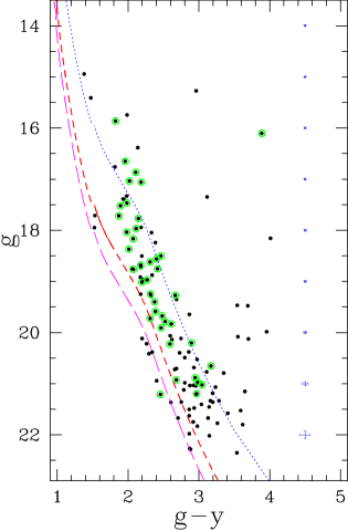
Figure 5: PS1 $g$ vs. $(g-y)$ CMD for the stars in the cluster region (black dots). The green circles are the member stars of the cluster. The curves denote a ZAMS derived from Pastorelli et al. (2019) corrected for extinction ($A_{V}$=2.9 mag) and distances of 1.75 kpc (blue-dotted curve, Bisht et al., 2017), 3.5 kpc (red-dashed curve, present analysis) and 4.5 kpc (purple-dashed curve, Cantat-Gaudin et al., 2018). Photometric error bars are also shown in the CMD.

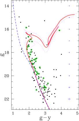
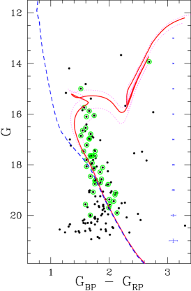
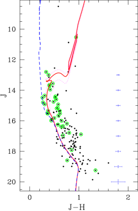
Figure 6: The CMDs generated from PS1 (left panel), $Gaia$ (middle panel), and TIRCAM2 (right panel) data for the stars in the cluster region. Symbols are as same as in Fig. 5. The blue dashed and solid red curves denote ZAMS and isochrone of age = 0.9 Gyr, respectively, derived from Pastorelli et al. (2019). The magenta dotted curves denote the isochrone of age = 0.8 Gyr (upper curve) and 1.2 Gyr (lower curve). All the curves are corrected for distance (3.5 kpc) and extinction ($A_{V}$=2.9 mag). Photometric error bars are also shown in the CMDs.

3.3 Distance and age of the cluster

Using the $Gaia$ data and maximum likelihood procedure, Cantat-Gaudin et al. (2018) have recently calculated the parallax and distance of this cluster as 0.195 mas and 4.5 kpc, respectively. However, they highlighted that the distances to clusters with mean parallaxes smaller than $\sim$0.2 mas would be better constrained by a Bayesian approach using priors based on an assumed density distribution of the Milky Way (Bailer-Jones et al., 2018) or photometric considerations (e.g., Anderson et al., 2018), or simply with more classical isochrone fitting methods (e.g., Phelps & Janes, 1994; Sharma et al., 2006; Sharma et al., 2017; Pandey et al., 2020a; Pandey et al., 2020b). Therefore, we have used both Bailer-Jones et al. (2018) approach and the isochrone fitting method to constrain the distance of this cluster.

The mean distance of the identified member stars of this cluster comes out to be $3.5\pm 0.9$ kpc (see, Bailer-Jones et al., 2018). This distance estimation is different from all the previous measurements of this cluster which places this cluster at a nearer distance (1.4 - 1.75 kpc, cf. Section 1) or a farther distance (4.5 kpc, Cantat-Gaudin et al., 2018). Therefore, to further check the validity of this distance (3.5 kpc), we have used the isochrone fitting method on the cluster CMD which is demonstrated successfully in many previous studies (cf., Phelps & Janes, 1994; Sharma et al., 2006; Sharma et al., 2017; Friel et al., 2014; Perren et al., 2015; Bossini et al., 2019; Pandey et al., 2020a; Pandey et al., 2020b). To fit the isochrone to the CMD, we need the information of reddening in the direction of the cluster. The MWSC provides the reddening value for this cluster as $A_{V}\sim$2.9 mag. Recently, using the $Gaia$ parallaxes and stellar photometry from PS1 and 2MASS, Green et al. (2019) have generated a three-dimensional map of dust reddening known as Bayestar dust map. We have used their map to estimate the reddening towards the direction of Cz3, which comes out to be similar to the MWSC estimate and this value has been used in the present analyses. The relative extinction values in different passbands thereafter have been estimated by using the relations given in Wang & Chen (2019).

In Fig. 5, we show the CMD of the stars located in the cluster region (black dots) using the PS1 data. The identified member stars are shown with green circles. We also show the zero-age main-sequence (ZAMS) generated from Pastorelli et al. (2019) for solar metallicity (z=0.02), corrected for reddening ($A_{V}\sim$2.9 mag) and distance of 1.75 kpc (blue-dotted curve, Bisht et al., 2017), 3.5 kpc (red-dashed curve, Bailer-Jones et al., 2018) and 4.5 kpc (purple-dashed curve, Cantat-Gaudin et al., 2018). The index $(g-y)$ has been used here because of having a very large colour range. The ZAMS is visually fitted to the lower envelop of the distribution of member stars where the bend occurs in the MS. This choice of visual fitting was dictated by several factors, such as, distribution of binary stars, rotation and evolutionary effects (see for details, Golay, 1974; Phelps & Janes, 1994). Clearly, out of the three ZAMSs corrected for different distance estimates, the member stars are best represented by the ZAMS corrected for a distance of 3.5 kpc. Here, it is worthwhile to note that the visual fitting in this case is prone to large error as we do not have the error estimates in the extinction values and the cluster can have differential/anomalous reddening. Therefore, we have assigned a distance of $3.5\pm 0.9$ kpc to Cz3 cluster from the distance estimate of its member stars by Bailer-Jones et al. (2018).

To derive the age of this cluster, we have used the deep multi-wavelength data from present observations, $Gaia$, and PS1, to generate CMDs in different colour spaces and are shown in Fig. 6. The CMDs display a well defined MS and a MS turn-off point. The ZAMS (generated from Pastorelli et al. (2019) for solar metallicity (z=0.02)) corrected for the cluster’s distance and reddening is also shown by a dashed blue curve. We can visually fit an isochrone of age $\sim$0.9 Gyr (red solid curve) taken from Pastorelli et al. (2019) to the distribution of stars in the post-MS phase in all the CMDs. For comparison, we have also plotted the isochrones of 0.8 Gyr and 1.2 Gyr in the CMDs corrected for the distance and reddening which can be assumed as upper and lower limits of the age estimation (see e.g., Phelps & Janes, 1994).

3.4 Mass function

Open clusters possess many favorable characteristics for MF studies, e.g., clusters contain an (almost) coeval set of stars at the same distance with the same metallicity; hence, difficulties such as complex corrections for stellar birth rates, life times, etc, associated with determining the MF from field stars are automatically removed. The MF is often expressed by a power law, $N(\log m)\propto m^{\Gamma}$ and the slope of the MF is given as:

$$\Gamma=d\log N(\log m)/d\log m$$ (9)

where $N(\log m)$ is the number of stars per unit logarithmic mass interval. The MS luminosity function (LF) obtained with the help of the CMD and corrected for the data incompleteness, has been converted into an MF using the isochrone of Pastorelli et al. (2019) of age $\sim$0.9 Gyr, corrected for the distance and extinction.

To derive the MF slopes of the lower mass end of a cluster, it is important to know the completeness limits of the photometric data. The photometric data may be incomplete due to various reasons (e.g., crowding of stars, the detection limit, background nebulosity, etc). To determine the completeness factor (CF) of the photometric data, we used the ADDSTAR routine of DAOPHOT II. This method has been used by various authors (see Sharma et al., 2007, 2008; Sharma et al., 2017; Pandey et al., 2020b, and references therein). Briefly, the method consists of randomly adding artificial stars of known magnitudes and positions into the original frame. The frames are reduced with the same procedure used for the original frame. The ratio of the number of stars recovered to those added in each magnitude interval gives the CF as a function of magnitude. The luminosity distribution of artificial stars is chosen in such a way that more stars are inserted into the fainter magnitude bins. In all, about 15 percent of the total stars are added so that the crowding characteristics of the original frame do not change significantly (see Sagar & Richtler, 1991).

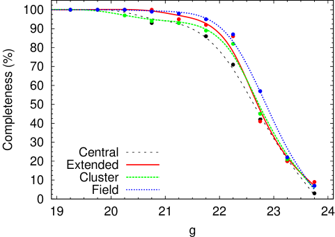
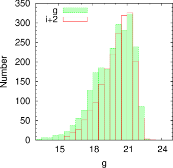
Figure 7: (Left panel): Completeness factor as a function of $g$ mag for different regions of the Cz3 cluster derived from the artificial star experiments (ADDSTAR, see Section 3.4 for details). The continuous curves are the smoothened bezier curves for the data points for completeness for different regions. (Right Panel): Histograms for the number of stars in different magnitude bins showing the limiting magnitude and completeness factor in PS1 $g$ and $i$ bands.

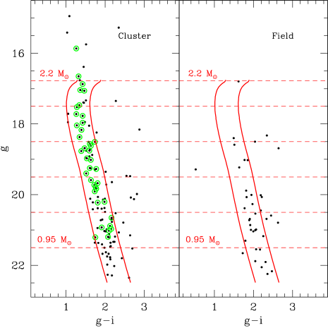
Figure 8: (Left panel): PS1 $g$ vs. $(g-i)$ CMDs for the stars in the cluster and field regions. The symbols are same as in figure 5. The curves denote a MS envelop created by the MS isochrone of 0.9 Gyr derived from Pastorelli et al. (2019) corrected for the distance (3.5 kpc) and extinction ($A_{V}$=2.6 mag (left curve) and $A_{V}$= 3.2 mag (right curve)). Upper and lower horizontal dashed lines represent the MS turn-off point and 90 percent completeness limit, respectively. (Right panel): A plot of the MF for the cluster, central and extended regions of Cz3 using PS1 data. Log $\phi$ represents log($N$/dlog $m$). Open circles represent data below 50 percent completeness limit and are not used in the MF analysis. The error bars represent $\pm\sqrt{N}$ errors. The solid line shows a least squares fit to the MF distribution (black filled circles).

Table 4: The mass function slopes for two sub-regions and for the whole cluster region in the given mass range.

Mass range	Mass Function slopes ($\Gamma$)
($M_{\odot}$)	Central region	Extended region	Cluster region
$2.2-0.95^{a}$	$0.21\pm 0.63$	$-2.20\pm 1.90$	$-1.01\pm 0.43$
$2.2-0.95^{b}$	$0.61\pm 0.87$	$-$	$-$

^a: PS1 data ^b: TIRCAM2 data

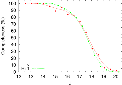
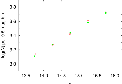
Figure 9: (Top panel): Completeness factor as a function of $J$ magnitude derived from the artificial star experiments (ADDSTAR, see Section 3.4 for details) on the TIRCAM2 $J$ and $H$ band images. The $H$-band completeness factor is off-setted by the mean colour of the MS stars (i.e., 1.0 mag). The continuous curves are the smoothened bezier curves for the data points for completeness. (Middle panel): A comparison of field stars distribution generated by using a nearby reference field (green filled circles) and by the model/simulations generated by the Besançon model (red open circles). (Bottom panel): A plot of the MF for member stars in the central region of the Cz3 cluster using TIRCAM2 data. Log $\phi$ represents log($N$/dlog $m$). The error bars represent $\pm\sqrt{N}$ errors. The solid line shows a least squares fit to the MF distribution (black filled circles).

We have used the deep PS1 photometric data to generate $g$ versus $(g-i)$ CMDs to derive MF slopes in the cluster as well as in the central and extended regions (cf. Fig. 3). Therefore, for the calculation of CF of this CMD we have used PS1 images in $g$ and $i$ bands. We first performed PSF photometry on these images. The detection threshold was chosen such that the detections are similar to that in the PS1 catalog. The instrumental magnitudes are then converted to the standard magnitudes by applying offsets determined by using the PS1 catalog. We have then added artificial stars in these images in such a way that they have similar geometrical locations but differ in $i$ brightness according to mean $(g-i)$ colours ($\sim$ 2 mag) of the MS stars. The minimum value of the CF of the pair thus obtained is used to correct the data for incompleteness. We have derived the CF for the central, extended, and field regions of Cz3 and is shown as a function of $g$-band in the left panel of Fig. 7. As expected the incompleteness of the data increases with increasing magnitude and stellar crowding. The photometric data is 90 percent complete upto 21.5 mag in the $g$-band which corresponds to a star of mass 0.95 M_⊙ at the distance of the Cz3 cluster. The PS1 median 50 percent completeness for the $g$-band is reported to be 23.2 mag, and the present estimates are more or less similar. As assumed in various previous studies, the peak of the observed LF can be considered as the 90 percent completeness limit of the data (cf. Evans et al., 2003; Willis et al., 2013; Jose et al., 2013; Jose et al., 2016; Sharma et al., 2016; Pandey et al., 2020b; Zhang et al., 2020). Therefore to further verify our CF values, we have constructed the LFs for $g$ and $i$ (off-setted by mean MS colour of 2 mag) bands and are shown in the right panel of Fig. 7. Both the distributions are showing a peak around 21.5 mag and thus agree with our estimated 90 percent CF value.

In the left panel of Fig. 8, we show the CMD for the cluster region as well as for the reference region ($\alpha_{J2000}$: $01^{h}04^{m}00^{s}.0$, $\delta_{J2000}$: $+62^{\circ}37^{\prime}28^{\prime\prime}$) having the same area. The contamination due to field stars is greatly reduced by selecting a sample of stars which are located near the well-defined MS (cf. Sharma et al., 2008). Therefore, we generated an envelope of $\pm 0.3$ mag around the CMD keeping in mind the distribution of member stars and is shown in the left panel of Fig. 8. As the MS is extended from $\sim$16.5 mag ($\sim$2.2 M_⊙) to $\sim$22.5 mag ($\sim$0.85 M_⊙), the number of probable cluster members were obtained by subtracting the contribution of field stars (corrected for data incompleteness), in different magnitude bins having size of 1.0 mag starting from $g=16.5$ mag, from the contaminated sample of MS stars (also corrected for data incompleteness). We have shown the MS turn-off point and 90 percent completeness limit in the left panel of Fig. 8. One member stars above the MS turn-off point could be a MS blue straggler star of the cluster. The resultant MF distributions for the cluster as well as the central and extended regions are shown in the right panel of Fig. 8. The values of the MF slopes are listed in Table 4.

We have also used the present deep NIR photometry taken from TIRCAM2 to derive MF slope of the central region of Cz3. The CF is determined for $J$ versus $J-H$ CMD using the same procedure as discussed above and is shown in the top panel of Fig. 9. To decontaminate the field star population, we have used the CMD of a nearby reference field taken from the 2MASS survey (for stars having $J<16$ mag) and the Besançon Galactic model of stellar population synthesis (Robin et al., 2003; Ojha et al., 2004) (for stars having $J>16$ mag). To check the accuracy of statistics of number of stars generated by the Besançon model, we have compared the LF generated from the model with that from the 2MASS survey ($J<16$ mag) in the middle panel of Fig. 9. The LFs from both methods are matching well and the resultant MF distribution is shown in the bottom panel of Fig. 9. The value of MF slope for the central region of Cz3 derived by using TIRCAM2 is listed in Table 4.

4 Discussion

It is well known that the internal interaction of two-body relaxation due to encounters among member stars and external tidal forces due to the Galactic disk or giant molecular clouds can further influence the structure of the clusters. The vast majority of Galactic open clusters do not survive longer than a few hundred million years (Wielen, 1971; Binney & Tremaine, 1987). Recently, Yeh et al. (2019) found that the 99 percent of the cluster mass of an old open cluster Ruprecht 147 (age = 2.5 Gyr) was lost due to tidal interaction with the Milky way. They have found prominent leading and trailing trails of stars along the cluster orbit, demonstrating that the cluster is losing stars at fast pace and is rapidly dissolving into Galactic disc. Signatures of dissolution can be seen in many Galactic open clusters in the form of truncated MS in the cluster’s CMD (Patat & Carraro, 1995; Piotto & Zoccali, 1999; Stolte et al., 2005), which, in turn, produce the MF peaked closer to higher mass stars. Also, the stellar distribution in several star clusters on the plane of the sky appears elongated or distorted (Yeh et al., 2019). We will discuss those effects in the Cz3 cluster to check its dynamical status in the following sub-sections.

4.1 Mass function and mass segregation

The higher mass stars mostly follow the Salpeter MF (Salpeter, 1955). At lower masses, the MF is less well constrained, but appears to flatten below 1 M_⊙ and exhibits fewer stars of the lowest masses (Kroupa, 2002; Chabrier, 2003; Lim et al., 2015; Luhman et al., 2016). In this study, we find a slight change of MF slope from the high to low mass end with a turn-off at around 1.5 M_⊙ for the cluster. This truncation of MF slope at a bit higher mass bins might be due to the escape of members from the cluster. We have also found that the MF slopes for the cluster region ($\Gamma=-1.01\pm 0.43$, cf. Table 4) is shallower than the Salpeter (1955) value i.e., $\Gamma$=-1.35, indicating the lack of low mass stars there. This lack of low mass stars can be also attributed to their escape from the cluster’s boundary. Stars escape from the parent cluster because of a variety of processes. They can be divided into internal, like two body relaxation and stellar evolution (Lamers et al., 2005; Dalessandro et al., 2015), and external, like tidal interaction and encounters with molecular clouds, spiral arms, the Galactic disc and, in general, the interactions with the Galactic tidal field (Danilov & Seleznev, 1994; Gieles et al., 2006; Gieles & Baumgardt, 2008; Yeh et al., 2019).

In Fig. 10, we show the CMDs of stars in the central and extended regions of the cluster. Clearly, there are many massive stars in the central region as compared to the extended region of the cluster. To investigate further, we look for the signature of mass segregation by checking the change of MF slope from the central region to the outer extended region of this cluster, which is in fact getting steeper in the extended region (cf. Table 4). This is an indicative of prevalent mass segregation in this cluster. To verify, we have also used Allison et al. (2009a) method of calculating mass segregation ratio (MSR) as a measure to identify and quantify mass segregation in the cluster. This method has been updated by Olczak et al. (2011) by using the geometric mean to minimize the influence of outliers. In this method, the minimal sampling tree (MST) for the $n_{MST}$ most massive stars is constructed and then the mean edge length $\gamma_{mp}$ is determined. The MST is defined as a network of branches connecting points such as the total length of the branches is minimized and there is no loops (Battinelli, 1991). This algorithm has lately become a popular tool to search for clusters of stars since it is independent from the star’s density number (Gutermuth et al., 2009; Chavarría et al., 2014; Sharma et al., 2016). We then constructed the MST of the randomly selected same number of stars from the entire sample and determed the mean edge length $\gamma_{rand}$. Thereafter, the value of the MSR ‘$\Gamma_{MSR}$’ (Olczak et al., 2011) is estimated as:

$$\Gamma_{MSR}={{\langle\gamma^{rand}_{MST}\rangle}\over{\gamma^{mp}_{MST}}},$$ (10)

and the associated standard deviation of $\Gamma_{MSR}$ is estimated as:

$$\Delta\Gamma_{MSR}=\Delta\gamma^{rand}_{MST}.$$ (11)

This is done 100 times in order to obtain ${\langle\gamma^{rand}_{MST}\rangle}$. A value of $\Gamma_{MSR}\approx 1$ indicates that the most massive and the randomly selected are distributed in a similar manner, whereas $\Gamma_{MSR}>1$ and $\Gamma_{MSR}\ll 1$ points toward mass segreegation and inverse mass segregation, respectively (Dib et al., 2018). Since, the Cz3 is an old cluster with negligible differential extinction, we use the magnitudes of member stars (cf. Section 3.2) as a proxy for the mass. By this, we can avoid the introduction of additional uncertainties of converting the observed luminosities into masses (Dib et al., 2018). We derived $\Gamma_{MSR}=1.2\pm 2.9$, which also suggests the effect of mass-segregation in this cluster. The large error in $\Gamma_{MSR}$ is may be due to a small mass range of this old cluster.

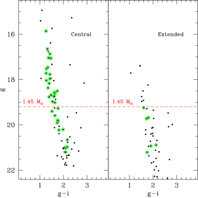
Figure 10: PS1 $g$ vs. $(g-i)$ CMDs for the stars in the central and extended regions of the cluster (black dots). Member stars are shown with green circles. The horizontal dashed line corresponds to the mass of the brightest star in the extended region identified as a cluster member by using PM data.

To decide whether mass segregation is primordial or due to dynamical relaxation, we have to estimate the dynamical relaxation time, $T_{E}$, the time in which the individual stars exchange sufficient energy so that their velocity distribution approaches that of a Maxwellian equilibrium using the method given by Binney & Tremaine (1987):

$$T_{E}={{N}\over{8logN}}\times T_{cross}$$ (12)

where $T_{cross}={D\over\sigma_{V}}$ denote the crossing time, $N$ is the total number of stars in the region under investigation of diameter D, and $\sigma_{V}$ is the velocity dispersion, with a typical value of 3 km s^-1 (Bisht et al., 2017). The estimated value of dynamical relaxation time, using the member stars (cf. Section 3.2), comes out to be $T_{E}\sim 10$ Myr for the Cz3 cluster. A comparison of cluster age (i.e. 0.9 Gyr) with its dynamical relaxation time indicates that the former is much greater than the latter, leading to the conclusion that this cluster is dynamically relaxed and the dynamical evolution of stars could be the reason for the observed mass segregation in this cluster. One of the consequences of this mass segregation process is that the lowest-mass members become the most vulnerable to be ejected out of the system (e.g., see Mathieu, 1984) This stellar evaporation, with an e-folding timescale of $\tau_{evap}\sim 100\times T_{E}$ (Shu, 1982; Binney & Tremaine, 1987), leads to a continuing decrease of the total mass, and hence the gravitational binding energy of the cluster. Any external disturbance, such as the tidal force from nearby giant molecular clouds or star clusters, passages through Galactic spiral arms or disks, or a shear force by Galactic differential rotation, exacerbates the disintegration of the cluster. As $\tau_{evap}$ comes out to be $\sim$1 Gyr for Cz3 having age$\sim$0.9 Gyr, this cluster can be considered as a probable candidate undergoing disintegration processes.

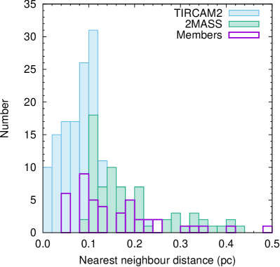
Figure 11: Histogram of the nearest neighbor (NN2) lengths for the stars in the cluster region of Cz3. The magenta, green and blue histograms represent Gaia, 2MASS and TIRCAM2 data, respectively (see the text for details).

4.2 Morphological structure

By analyzing the stellar density distribution morphology, observational analyses can address the link between star formation, gas expulsion, and the dynamics of the clusters, as well as how these processes guide the evolution of clusters (Gutermuth et al., 2005). From the isodensity contours (cf. Section 3.1), we have found that this cluster is showing elongated morphology. We will now derive the Q parameter of the sample of cluster members identified in the Section 3.2. The Q parameter is generally used to distinguish between clusters with a central density concentration and hierarchical clusters with a fractal substructure (cf. Cartwright & Whitworth, 2004, 2009), to quantify the structure of this cluster. The Q parameter ($Q={{\bar{l}_{MST}}\over{\bar{s}}}$) combines the normalized correlation length $\bar{s}$ i.e. the mean distance between all stars, and the normalized mean edge length $\bar{l}_{MST}$ derived from the MST. The MST mean branches length ‘$l_{MST}$’ is calculated directly from the MST total length divided by the number of branches ‘N’ minus 1. Then, it is normalized by $\sqrt{A_{cluster}/N}$. In a similar way, the mean separation between points ‘$s$’ is normalized by $R_{cluster}$. Using the normalized values $\bar{l}_{MST}$ and $\bar{s}$, the Q parameter becomes independent from the cluster size (Schmeja & Klessen, 2006). According to Cartwright & Whitworth (2004), both $\bar{l}_{MST}$ and $\bar{s}$ values decrease as the degree of radial concentration increases (or the level of hierarchy decreases). However, $\bar{s}$ decreases faster than $\bar{l}_{MST}$. This way, a group of $(x_{N},y_{N})$ points distributed radially will have a high Q value (Q $>$ 0.8) while clusters with a more fractal distribution will have a low Q value (Q $<$ 0.8) (Cartwright & Whitworth, 2004; Chavarría et al., 2014). We have found Q=0.75, for the member stars of the Cz3 cluster (cf. Section 3.2) in the magnitude range $15>G>19$ mag, indicating fractal distribution of stars in this cluster. This is in agreement with our isodensity contour structures having two peaks in the cluster region.

The dynamical evolution of stars in a region can also be analyzed by deriving the typical spacing between them and comparing this spacing to the Jean’s fragmentation scale for a self-gravitating medium with thermal pressure (Gomez & Llibre, 1983). We measured the projected distance from each star to its nearest star neighbor (NN2) and plotted their histograms with a bin size of 0.02 pc in Fig. 11, for the stars in the cluster region from the TIRCAM2 as well as from the 2MASS data and, for the Gaia identified members stars (cf. Section 3.2). The TIRCAM2 sample shows a smaller NN2 distance distribution as compared to 2MASS data, may be due to a better resolution of the present TIRCAM2 observations, but, all the histograms are showing a major peak in their distribution at $\sim$0.1 pc with a long tail at larger distances. Gutermuth et al. (2009), in their study of NN2 spacing’s of stellar sources in 36 young star-forming clusters, found a well-defined peak at 0.02-0.05 pc and a tail extending to the spacings of 0.2 pc or greater. Recently, Sharma et al. (2016) also found a well-defined single peak around 0.03 pc with extended spacing upto 1 pc in their histogram of NN2 spacings of stellar sources in a sample of eight bright-rimmed clouds (BRCs). NN2 spacings of stellar sources in young star-forming regions having a well-defined single peak at smaller spacing (0.03-0.05 pc) indicate a significant degree of Jean’s fragmentation, whereas in the Cz3 cluster case, which is comparatively an older cluster, the peak of similar distribution at a larger distance ($\sim$0.1 pc) indicates a role of stellar dynamics in the structural evolution of this cluster.

We have also calculated the mean ($\sim$17 stars/pc²) and peak ($\sim$100 stars/pc²) stellar densities in this cluster using the position of members stars of this cluster (cf. Section 3.2) by using NN based technique discussed in Section 3.1. Chavarría et al. (2014) and Gutermuth et al. (2009), have derived mean stellar densities as 33 and 60 stars/pc² and the peak stellar densities as 150 and 200 stars/pc², respectively, for their samples of embedded clusters. Recently, Sharma et al. (2016) also found similar values for the mean ($\sim$60 stars/pc²) and peak ($\sim$150 stars/pc²) stellar densities in the core region of a sample of eight BRCs.

The tidal radius of a star cluster in the solar neighborhood is computed by using the equation given by Pinfield et al. (1998):

$$r_{t}=\left\{{{GM_{C}}\over{2(A-B)^{2}}}\right\}^{1/3}$$ (13)

where $G$ is the gravitational constant, $M_{C}$ is the total mass of the cluster, and $A$ and $B$ are the Oort constants, $A=15.3\pm 0.4$ kms^-1 kpc^-1, $B=−11.9\pm 0.4$ kms^-1 kpc^-1 (Bovy, 2017). Upto the completeness limit of the present photometric data i.e. 0.95 M_⊙, the mass of the cluster is estimated as $M_{C}$ = 89 M_⊙ from the MF distribution of the cluster stars as derived from the LF of the member stars (cf. Section 3.4). The corresponding tidal radius comes out to be $6.4\pm 0.2$ pc. This is a good approximation even if we have missed 50 percent of the cluster mass in the lower mass bins due to data incompleteness. The tidal radius will not change much as the resultant tidal radius then will be $\sim$8 pc. Therefore, we can conclude that the tidal radius ($r_{t}\sim$6.4 pc) of this cluster is much larger than the present estimate of the cluster radius ($R_{cluster}\sim$1.2 pc). Usually, the cluster boundary is taken as one tidal radius, as in the case of Blanco 1 (Zhang et al., 2020) or Coma Bernices (Tang et al., 2019). But, there are some studies (see e.g., Röser et al., 2019), in which the cluster boundary of 2 tidal radii was adopted. Also the Cz3 cluster is showing elongated structure and the extended tail like structure might be caused by tidal forces from a nearby massive object, by disk crossing, or by differential rotation in the disk. Tidal stripping depends on the mass and also on the age of a cluster, e.g., the ratio of the members inside the tidal radius to those outside for a young ($\sim 100$ Myr) cluster Blanco is reported to be 3 (Zhang et al., 2020). Whereas, for a cluster with age $\sim 700$ Myr, Coma Berenices, this ratio comes out to be 0.6 (Tang et al., 2019). For an old ($\sim 800$ Myr) but a massive cluster, Hyades, this ratio is $\sim 1.1$ (Röser et al., 2019).

Therefore, the observed small size of this old ($\sim 0.9$ Gyr) cluster looks like the remain of a cluster which has already lost many of its member stars. The shallow MF slope, signature of mass-segregation, low density/large separation of stars, elongated and distorted morphologies of this dynamically relaxed cluster ($T_{E}=10$ Myr), indicate that the Cz3 ($age=0.9$ Gyr) is a loosely bound old cluster which may be under the process of dissolution under the influence of external tidal interactions.

5 Summary and Conclusion

We have performed a detailed analysis of the Cz3 open cluster using deep NIR observations taken from TIRCAM2 on 3.6m DOT along with the recently available high quality PM data from the Gaia DR2 and deep photometric data from PS1. We have investigated the structure of this cluster, determined the membership probability of stars in the cluster region, derived the fundamental parameters of the cluster, and studied the MF and mass segregation in this cluster. The main results of this study can be summarized as follows:

• We have derived the structural parameters of this cluster by using isodensity contours and found that the Cz3 cluster is showing an elongated morphology. The area of this cluster from PS1 data is estimated as 4.35 arcmin square which corresponds to a circular radius of 1.18 arcmin (1.2 pc). The core radius of this cluster is found to be 30 arcsec ($\sim$0.5 pc).

• Using Gaia DR2 data, 45 stars were marked as highly probable cluster members. We have estimated the distance of this cluster both using parallax of member stars and the CMD fitting technique and found that the cluster is located at a distance of $3.5\pm 0.9$ kpc. We have also estimated the age of this cluster as $0.9^{+0.3}_{-0.1}$ Gyr.

• We have derived the MF slope ($\Gamma$) in the cluster region in the mass range $\sim$0.95$<$M/M_⊙$<$2.2 as $-1.01\pm 0.43$, which is shallower than the value ‘-1.35’ given by Salpeter (1955). The cluster is showing a signature of mass-segregation and the dynamical age of this cluster is found to be much less than the age of the cluster, indicating that this cluster is dynamically relaxed.

• The Q parameter value for this cluster suggests a fractal distribution of stars in this cluster which is in agreement with isodensity contour structures showing elongated morphology with two peaks. We have found a major peak in the NN2 distance distribution of the stars in this cluster at $\sim$0.1 pc, which is larger than that of stars in young star-forming regions ($\sim$0.03-0.05 pc).

Finally, from the observed, small size of this old ($\sim$0.9 Gyr) cluster as compare to its tidal radius, shallow MF slope, signature of mass-segregation, low density/large separation of stars, elongated and distorted morphology, dynamical relaxation time ($T_{E}$=10 Myr) compared to the age of Cz3 (age=0.9 Gyr), we conclude that the Cz3 is a loosely bound old disintegrating cluster under the influence of external tidal interactions.

Data availability

The data underlying this article are available in the article and in its online supplementary material.

References

- Allison et al. (2009a) Allison R. J., Goodwin S. P., Parker R. J., Portegies Zwart S. F., de Grijs R., Kouwenhoven M. B. N., 2009a, MNRAS, 395, 1449
- Allison et al. (2009b) Allison R. J., Goodwin S. P., Parker R. J., de Grijs R., Portegies Zwart S. F., Kouwenhoven M. B. N., 2009b, ApJ, 700, L99
- Allison et al. (2010) Allison R. J., Goodwin S. P., Parker R. J., Portegies Zwart S. F., de Grijs R., 2010, MNRAS, 407, 1098
- Anderson et al. (2018) Anderson L., Hogg D. W., Leistedt B., Price-Whelan A. M., Bovy J., 2018, AJ, 156, 145
- Bailer-Jones et al. (2018) Bailer-Jones C. A. L., Rybizki J., Fouesneau M., Mantelet G., Andrae R., 2018, AJ, 156, 58
- Balaguer-Núnez et al. (1998) Balaguer-Núnez L., Tian K. P., Zhao J. L., 1998, A&AS, 133, 387
- Battinelli (1991) Battinelli P., 1991, A&A, 244, 69
- Baug et al. (2018) Baug T., et al., 2018, Journal of Astronomical Instrumentation, 7, 1850003
- Bellini et al. (2009) Bellini A., et al., 2009, A&A, 493, 959
- Binney & Tremaine (1987) Binney J., Tremaine S., 1987, Galactic dynamics (Princeton, NJ: Princeton Univ. Press)
- Bisht et al. (2017) Bisht D., Yadav R. K. S., Durgapal A. K., 2017, New Astron., 52, 55
- Bonatto et al. (2006) Bonatto C., Kerber L. O., Bica E., Santiago B. X., 2006, A&A, 446, 121
- Bonnell et al. (1998) Bonnell I. A., Bate M. R., Zinnecker H., 1998, MNRAS, 298, 93
- Bossini et al. (2019) Bossini D., et al., 2019, A&A, 623, A108
- Bovy (2017) Bovy J., 2017, MNRAS, 468, L63
- Brandl et al. (1999) Brandl B., Brandner W., Eisenhauer F., Moffat A. F. J., Palla F., Zinnecker H., 1999, A&A, 352, L69
- Brinkmann et al. (2017) Brinkmann N., Banerjee S., Motwani B., Kroupa P., 2017, A&A, 600, A49
- Cantat-Gaudin et al. (2018) Cantat-Gaudin T., et al., 2018, VizieR Online Data Catalog, pp J/A+A/618/A93
- Cartwright & Whitworth (2004) Cartwright A., Whitworth A. P., 2004, MNRAS, 348, 589
- Cartwright & Whitworth (2009) Cartwright A., Whitworth A. P., 2009, MNRAS, 392, 341
- Chabrier (2003) Chabrier G., 2003, PASP, 115, 763
- Chambers et al. (2016) Chambers K. C., et al., 2016, arXiv e-prints, p. arXiv:1612.05560
- Chavarría et al. (2014) Chavarría L., Allen L., Brunt C., Hora J. L., Muench A., Fazio G., 2014, MNRAS, 439, 3719
- Cutri et al. (2003) Cutri R. M., et al., 2003, VizieR Online Data Catalog, 2246, 0
- Dalessandro et al. (2015) Dalessandro E., Ferraro F. R., Massari D., Lanzoni B., Miocchi P., Beccari G., 2015, ApJ, 810, 40
- Danilov & Seleznev (1994) Danilov V. M., Seleznev A. F., 1994, Astronomical and Astrophysical Transactions, 6, 85
- Dias et al. (2002) Dias W. S., Alessi B. S., Moitinho A., Lépine J. R. D., 2002, A&A, 389, 871
- Dib (2007) Dib S., 2007, Journal of Korean Astronomical Society, 40, 157
- Dib et al. (2008) Dib S., Brandenburg A., Kim J., Gopinathan M., André P., 2008, ApJ, 678, L105
- Dib et al. (2010) Dib S., Hennebelle P., Pineda J. E., Csengeri T., Bontemps S., Audit E., Goodman A. A., 2010, ApJ, 723, 425
- Dib et al. (2011) Dib S., Piau L., Mohanty S., Braine J., 2011, MNRAS, 415, 3439
- Dib et al. (2013) Dib S., Gutkin J., Brandner W., Basu S., 2013, MNRAS, 436, 3727
- Dib et al. (2018) Dib S., Schmeja S., Parker R. J., 2018, MNRAS, 473, 849
- Evans et al. (2003) Evans II N. J., et al., 2003, PASP, 115, 965
- Friel et al. (2014) Friel E. D., et al., 2014, A&A, 563, A117
- Gaia Collaboration et al. (2016) Gaia Collaboration et al., 2016, A&A, 595, A1
- Gaia Collaboration et al. (2018) Gaia Collaboration et al., 2018, A&A, 616, A1
- Gieles & Baumgardt (2008) Gieles M., Baumgardt H., 2008, MNRAS, 389, L28
- Gieles et al. (2006) Gieles M., Portegies Zwart S. F., Baumgardt H., Athanassoula E., Lamers H. J. G. L. M., Sipior M., Leenaarts J., 2006, MNRAS, 371, 793
- Girard et al. (1989) Girard T. M., Grundy W. M., Lopez C. E., van Altena W. F., 1989, AJ, 98, 227
- Golay (1974) Golay M., 1974, Introduction to astronomical photometry, doi:10.1007/978-94-010-2169-2.
- Gomez & Llibre (1983) Gomez G., Llibre J., 1983, in Markellos V. V., Kozai Y., eds, Astrophysics and Space Science Library Vol. 106, IAU Colloq. 74: Dynamical Trapping and Evolution in the Solar System. pp 325–338, doi:10.1007/978-94-009-7214-8_34
- Green et al. (2019) Green G. M., Schlafly E., Zucker C., Speagle J. S., Finkbeiner D., 2019, ApJ, 887, 93
- Gutermuth et al. (2005) Gutermuth R. A., Megeath S. T., Pipher J. L., Williams J. P., Allen L. E., Myers P. C., Raines S. N., 2005, ApJ, 632, 397
- Gutermuth et al. (2009) Gutermuth R. A., Megeath S. T., Myers P. C., Allen L. E., Pipher J. L., Fazio G. G., 2009, ApJS, 184, 18
- Hoffman et al. (1983) Hoffman G. L., Salpeter E. E., Wasserman I., 1983, ApJ, 268, 527
- Jose et al. (2013) Jose J., et al., 2013, MNRAS, 432, 3445
- Jose et al. (2016) Jose J., Kim J. S., Herczeg G. J., Samal M. R., Bieging J. H., Meyer M. R., Sherry W. H., 2016, ApJ, 822, 49
- Kharchenko et al. (2012) Kharchenko N. V., Piskunov A. E., Schilbach E., Röser S., Scholz R.-D., 2012, A&A, 543, A156
- Kharchenko et al. (2013) Kharchenko N. V., Piskunov A. E., Schilbach E., Röser S., Scholz R.-D., 2013, A&A, 558, A53
- Kholopov (1969) Kholopov P. N., 1969, Soviet Ast., 12, 625
- Kroupa (2002) Kroupa P., 2002, Science, 295, 82
- Kruijssen (2012) Kruijssen J. M. D., 2012, MNRAS, 426, 3008
- Kumar et al. (2018) Kumar B., et al., 2018, Bulletin de la Societe Royale des Sciences de Liege, 87, 29
- Lada & Lada (2003) Lada C. J., Lada E. A., 2003, ARA&A, 41, 57
- Lamers et al. (2005) Lamers H. J. G. L. M., Gieles M., Portegies Zwart S. F., 2005, A&A, 429, 173
- Lim et al. (2015) Lim B., Sung H., Hur H., Park B.-G., 2015, arXiv e-prints, p. arXiv:1511.01118
- Luhman et al. (2016) Luhman K. L., Esplin T. L., Loutrel N. P., 2016, ApJ, 827, 52
- Mathieu (1984) Mathieu R. D., 1984, ApJ, 284, 643
- McMillan et al. (2007) McMillan S. L. W., Vesperini E., Portegies Zwart S. F., 2007, ApJ, 655, L45
- Mermilliod (2000) Mermilliod J.-C., 2000, in Pallavicini R., Micela G., Sciortino S., eds, Astronomical Society of the Pacific Conference Series Vol. 198, Stellar Clusters and Associations: Convection, Rotation, and Dynamos. p. 105
- Naik et al. (2012) Naik M. B., et al., 2012, Bulletin of the Astronomical Society of India, 40, 531
- Ojha et al. (2004) Ojha D. K., et al., 2004, ApJ, 616, 1042
- Olczak et al. (2011) Olczak C., Spurzem R., Henning T., 2011, A&A, 532, A119
- Pandey et al. (1990) Pandey A. K., Mahra H. S., Sagar R., 1990, AJ, 99, 617
- Pandey et al. (2020a) Pandey A. K., Sharma S., Kobayashi N., Sarugaku Y., Ogura K., 2020a, MNRAS, 492, 2446
- Pandey et al. (2020b) Pandey R., et al., 2020b, ApJ, 891, 81
- Parker (2014) Parker R. J., 2014, MNRAS, 445, 4037
- Parker & Dale (2013) Parker R. J., Dale J. E., 2013, MNRAS, 432, 986
- Parker & Meyer (2012) Parker R. J., Meyer M. R., 2012, MNRAS, 427, 637
- Pastorelli et al. (2019) Pastorelli G., et al., 2019, MNRAS, 485, 5666
- Patat & Carraro (1995) Patat F., Carraro G., 1995, A&AS, 114, 281
- Perren et al. (2015) Perren G. I., Vázquez R. A., Piatti A. E., 2015, A&A, 576, A6
- Pfalzner & Kaczmarek (2013) Pfalzner S., Kaczmarek T., 2013, A&A, 559, A38
- Phelps & Janes (1994) Phelps R. L., Janes K. A., 1994, ApJS, 90, 31
- Pinfield et al. (1998) Pinfield D. J., Jameson R. F., Hodgkin S. T., 1998, MNRAS, 299, 955
- Piotto & Zoccali (1999) Piotto G., Zoccali M., 1999, A&A, 345, 485
- Robin et al. (2003) Robin A. C., Reylé C., Derrière S., Picaud S., 2003, A&A, 409, 523
- Röser et al. (2019) Röser S., Schilbach E., Goldman B., 2019, A&A, 621, L2
- Sagar & Richtler (1991) Sagar R., Richtler T., 1991, A&A, 250, 324
- Salpeter (1955) Salpeter E. E., 1955, ApJ, 121, 161
- Sariya et al. (2012) Sariya D. P., Yadav R. K. S., Bellini A., 2012, A&A, 543, A87
- Sariya et al. (2017) Sariya D. P., Jiang I.-G., Yadav R. K. S., 2017, AJ, 153, 134
- Schmeja & Klessen (2006) Schmeja S., Klessen R. S., 2006, A&A, 449, 151
- Schmeja et al. (2014) Schmeja S., Kharchenko N. V., Piskunov A. E., Röser S., Schilbach E., Froebrich D., Scholz R.-D., 2014, A&A, 568, A51
- Scholz et al. (2015) Scholz R.-D., Kharchenko N. V., Piskunov A. E., Röser S., Schilbach E., 2015, A&A, 581, A39
- Sharma et al. (2006) Sharma S., Pandey A. K., Ogura K., Mito H., Tarusawa K., Sagar R., 2006, AJ, 132, 1669
- Sharma et al. (2007) Sharma S., Pandey A. K., Ojha D. K., Chen W. P., Ghosh S. K., Bhatt B. C., Maheswar G., Sagar R., 2007, MNRAS, 380, 1141
- Sharma et al. (2008) Sharma S., Pandey A. K., Ogura K., Aoki T., Pandey K., Sandhu T. S., Sagar R., 2008, AJ, 135, 1934
- Sharma et al. (2016) Sharma S., et al., 2016, AJ, 151, 126
- Sharma et al. (2017) Sharma S., Pandey A. K., Ojha D. K., Bhatt H., Ogura K., Kobayashi N., Yadav R., Pandey J. C., 2017, MNRAS, 467, 2943
- Shu (1982) Shu F. H., 1982, The Physical Universe (Mill Valley, CA: Univ. Science Books)
- Spitzer & Harm (1958) Spitzer Jr. L., Harm R., 1958, ApJ, 127, 544
- Stolte et al. (2005) Stolte A., Brandner W., Grebel E. K., Lenzen R., Lagrange A.-M., 2005, ApJ, 628, L113
- Tang et al. (2019) Tang S.-Y., et al., 2019, ApJ, 877, 12
- Wang & Chen (2019) Wang S., Chen X., 2019, ApJ, 877, 116
- Wielen (1971) Wielen R., 1971, A&A, 13
- Willis et al. (2013) Willis S., Marengo M., Allen L., Fazio G. G., Smith H. A., Carey S., 2013, ApJ, 778, 96
- Yadav et al. (2013) Yadav R. K. S., Sariya D. P., Sagar R., 2013, MNRAS, 430, 3350
- Yang et al. (2013) Yang S.-C., Sarajedini A., Deliyannis C. P., Sarrazine A. R., Kim S. C., Kyeong J., 2013, ApJ, 762, 3
- Yeh et al. (2019) Yeh F.-C., Carraro G., Montalto M., Seleznev A. F., 2019, arXiv e-prints,
- Zhang et al. (2020) Zhang Y., Tang S.-Y., Chen W. P., Pang X., Liu J. Z., 2020, ApJ, 889, 99