Adversarial Examples on Object Recognition: A Comprehensive Survey

Abstract.

Deep neural networks are at the forefront of machine learning research. However, despite achieving impressive performance on complex tasks, they can be very sensitive: small perturbations of inputs can be sufficient to induce incorrect behavior. Such perturbations, called adversarial examples, are intentionally designed to test the network’s sensitivity to distribution drifts. Given their surprisingly small size, a wide body of literature conjectures on their existence and how this phenomenon can be mitigated. In this paper we discuss the impact of adversarial examples on security, safety and robustness of neural networks. We start by introducing the hypotheses behind their existence, the methods used to construct or protect against them and the capacity to transfer adversarial examples between different machine learning models. Altogether, the goal is to provide a comprehensive and self-contained survey of this growing field of research.

1. Introduction

There is no doubt Machine Learning (ML) and, in particular, Deep Neural Networks achieve impressive results on tasks where it is not possible to specify procedural rule-sets. Some examples are object recognition (He et al., 2016), machine translation (Sutskever et al., 2014) or speech recognition (Vaswani et al., 2017). Fueled by the increasing size of available data and a decrease in computing cost, ML algorithms are explored in a variety of new tasks and commercial applications, many of which are safety- and mission-critical.

Facing commercial deployment and the possibility of use in safety-critical systems, new properties of ML algorithms become important: in particular, their ability to maintain performance whenever faced with data coming from slightly different distributions than trained with or cope with uncertainties in the operational environment. These properties are defined as the algorithm’s power to generalize outside the training data and, respectively, the algorithm’s robustness.

In optimization, a robust solution has the ability to perform well under a certain level of uncertainty (Ben-Tal et al., 2009). Recent publications (Szegedy et al., 2013; Papernot et al., 2016a) showed ML algorithms exhibit low robustness and triggered an impressive wave of publications. Notably, DNNs are highly sensitive to small, intentional, distribution drifts – inputs which substantially decrease their performance, while being in close resemblance to training data. The term adversarial examples was first used to describe such inputs by Szegedy et al. (Szegedy et al., 2013).

Since an intention is required, many publications claim security consequences, e.g. (Nguyen et al., 2015; Kurakin et al., 2016b; Guo et al., 2018; Papernot et al., 2017; Su et al., 2019; Hein and Andriushchenko, 2017; Sinha et al., 2018b; Fawzi et al., 2018a), and hypothesize that commercial deployment is hindered by low robustness. In contrast, other publications show these claims are sometimes exaggerated and demand that clear security requirements are formulated before security consequences are claimed (Gilmer et al., 2018a; Carlini et al., 2019). In between, many publications investigate the existence of adversarial examples from a theoretical perspective and shed light on this particular behavior of ML algorithms. Overall, there are two emergent reasons to study adversarial examples: (1) because attackers might use them to exploit ML algorithms and (2) because they show ML algorithms are not robust, which may stop them from being adopted in some domains.

Another phenomenon presented in this paper is the potential to transfer adversarial examples between different ML algorithms. This means an input designed to fool DNNs can trigger the same behavior for kernel methods. From a security standpoint, this phenomenon suggests an attacker does not need precise information about the algorithm she plans to attack. Moreover, from a learning theory standpoint it suggests that (1) algorithms extrapolate similar decision boundaries despite using different ML constructs and (2) sensitivity to similar distribution drifts is an universal phenomenon, independent of the ML algorithm.

The goal of this paper is to provide a comprehensive survey of this research field. We characterize the phenomenon of adversarial examples from its inception by discussing its causes, position it in the context of security with relevant threat models, introduce methods to construct and defend against adversarial examples and explore the capacity to transfer them between different ML algorithms. We strive for completeness, but given the high activity on this topic, with new papers constantly coming out, there will be further improvements in attacks and defences which are not covered here. Nonetheless, the most representative attacks and defenses, which reveal how broad this research field is and how distinct the proposed solutions are, can be found in this paper. The taxonomies used and the different perspectives on security, safety and robustness discussed in this paper equip the reader with a broad framework in which new developments will fit. Altogether, the goal is to provide enough information so this document becomes a self-contained survey of the field, able to capture its different nuances and inspire new research directions.

Although adversarial examples can be found for a variety of tasks, we restrict our presentation to object recognition because (1) most publications target this task and (2) examples from this field are easier to illustrate. Nevertheless, adversarial example are constantly explored in other tasks. Of particular interest is malware detection (Grosse et al., 2016; Hu and Tan, 2017; Laskov et al., 2014; Xu et al., 2016; Kreuk et al., 2018) because it implies direct consequences on security. Other tasks such as reinforcement learning (Behzadan and Munir, 2017; Huang et al., 2017b; Lin et al., 2017), speech recognition (Carlini et al., 2016; Carlini and Wagner, 2018), facial recognition (Sharif et al., 2016), semantic segmentation (Xie et al., 2017) or video processing (Wei et al., 2018; Li et al., 2018; Thys et al., 2019) are also explored. Moreover, some practical experiments are not covered in detail, e.g. deploying adversarial examples in the physical world by printing corrupted images (Evtimov et al., 2017; Kurakin et al., 2016a), altering the image acquisition device (e.g. a phone camera) (Moosavi-Dezfooli et al., 2017a) or playing adversarial examples through speakers (Yakura and Sakuma, 2018).

A general remark about the terminology used in the paper: we make a distinction between ML algorithms and ML systems, in which the latter is any type of system which uses ML algorithms and other components. Whenever we talk about security, we consider the entire system under attack. Moreover, the terms ML algorithms and ML models are used with the same meaning. The rest of the paper is organized as follows. Section 2 provides some background information on machine learning, a formal definition of adversarial examples and positions the phenomenon in its historical context. Section 3 presents taxonomies for attacks and defenses and uses these to classify existing approaches from the literature. Section 4 discusses the property of robustness and Section 5 the hypotheses concerning the existence of adversarial examples. Sections 6 and 7 introduce the methods used to generate adversarial examples or protect against them, followed by the phenomenon of transferability in Section 8. We conclude with a discussion in Section 9 and lay down directions for future research in Section 10.

2. Background and Related Work

Prerequisites

A computer is said to learn from experience w.r.t. a task and a performance measure if its measured performance on the task increases with experience  (Mitchell et al., 1997). In this paper, we focus on the task of object recognition: given a set of images defined on the input space ${\mathcal{X}}$ with their labels from the output space ${\mathcal{Y}}$, sampled from a fixed, but unknown probability distribution ${\mathcal{D}}$ over the space ${\mathcal{Z}}={\mathcal{X}}\times{\mathcal{Y}}$, a ML algorithm attempts to find a mapping $f:{\mathcal{X}}\rightarrow{\mathcal{Y}}$ which minimizes the number of misclassified images. We assume that ${\mathcal{X}}$ is a metric space and we can define distance functions between two points of the space. The error made by a prediction $f({\bm{x}}_{i})=\hat{y_{i}}$ when the true label is $y_{i}$ is measured by a loss function $l:{\mathcal{Y}}\times{\mathcal{Y}}\rightarrow{\mathbb{R}}$. Through learning, we select a function $f^{*}$ from a hypotheses space ${\mathcal{F}}$ such that the expected loss $r(f)=\mathbb{E}_{({\bm{x}},y\sim{\mathcal{D}})}[l(f({\bm{x}}),y)]$ is minimal: $f^{*}=\operatorname*{arg\,min}_{f\in{\mathcal{F}}}r(f)$. In practice, ${\mathcal{D}}$ is not known and only a set of samples ${\mathcal{S}}$ (defined as a set of pairs $\{({\bm{x}}_{i},y_{i})\}_{i=1}^{n}$) is available for training. Thus, a ML algorithm uses the empirical loss to approximate the expected loss:

(1) $$\hat{f}=\operatorname*{arg\,min}_{f\in{\mathcal{F}}}\quad\mathbb{E}_{({\bm{x}},y)\sim{\mathcal{S}}}[l(f({\bm{x}}),y)].$$

The hypotheses space ${\mathcal{F}}$ can be any mapping from ${\mathcal{X}}$ to ${\mathcal{Y}}$ such as a linear function or a DNN. Choosing ${\mathcal{F}}$ for a task adds an inductive bias from the algorithm designer and involves a tradeoff between expressivity and generalization: if ${\mathcal{F}}$ is not expressive enough, the algorithm will not be able to learn complex hypotheses. On the opposite, if ${\mathcal{F}}$ is too expressive, the algorithm will overfit on the training data. The loss function is generally chosen to be zero when $f({\bm{x}}_{i})=y_{i}$ and positive otherwise. A common loss function for object recognition is the cross-entropy loss.

The Probably Approximately Correct (PAC) (Valiant, 1984) theoretical model for statistical learning guarantees that given enough samples for a desired accuracy $\epsilon$ and for the probability of getting non-representative samples from the training distribution $\delta$ ($0<\epsilon,\delta<1$), the empirical risk will have an error less than or equal to $\epsilon$ with probability $1-\delta$: $P(|r(\hat{f})-r(f^{*})|\leq\epsilon)\geq 1-\delta$. In this framework, given the choice for $\epsilon$ and $\delta$, we can derive the sample complexity for learning a hypothesis with minimal risk. An important assumption of this model is that training, test and inference data are drawn from the same probability distribution ${\mathcal{D}}$. Moreover, all data are sampled independently from distribution ${\mathcal{D}}$ (also called independent and identically distributed (i.i.d)).

Adversarial Examples.

Adversarial examples are inputs intentionally designed to be in close resemblance with samples from the distribution ${\mathcal{D}}$, but cause a misclassification. Formally, given a classification function $f$ and a clean sample ${\bm{x}}$, which gets correctly classified by $f$ with label $y$, an adversarial example ${\bm{x}^{\prime}}$ is constructed by applying the minimal perturbation $\eta$ to input ${\bm{x}}$ such that ${\bm{x}^{\prime}}$ gets classified with a different label $\hat{y}$: $\operatorname*{arg\,min}_{\eta}f({\bm{x}}+\eta)=\hat{y}$. Similarly, in the initial paper on adversarial examples, Szegedy et al. (Szegedy et al., 2013) search for the perturbation solving the following optimization problem:

(2) $$\min_{{\bm{x}^{\prime}}}. \|{\bm{x}^{\prime}}-{\bm{x}}\|_{p},$$

$$s.t. f({\bm{x}^{\prime}})=\hat{y},$$

where $||\cdot\|_{p}$ is a distance function defined on the metric space ${\mathcal{X}}$. Searching for the minimal perturbation is often a complex task because the search space is non-linear and non-convex (Papernot et al., 2017; Larochelle et al., 2009). However, many approximation solutions have been proposed. Finding solutions to eq. (LABEL:eq:adversarial_generic) is illustrated in Figure 1. Some examples of perturbations are also illustrated in Figure 2.

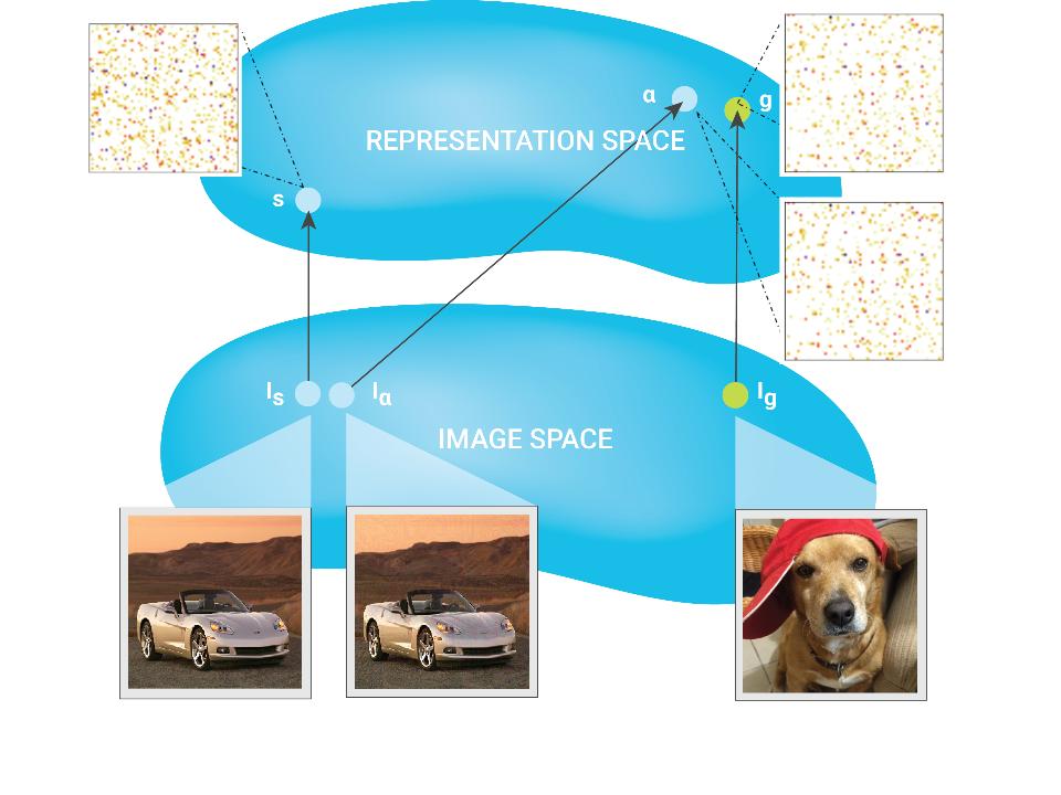
Figure 1. Adversarial example in input and representation space (Sabour et al., 2015). While the two pictures of cars are similar in the image space, the activation patterns of the second car are close to the activation patterns of the dog. Therefore, the second car gets classified as a dog. Moving the activation patterns from cars to dogs while keeping the representation in the image space similar is equivalent to searching for a solution to eq. (LABEL:eq:adversarial_generic) and generating an adversarial example.

The distance function most commonly used for adversarial examples in the object recognition domain is the p-norm:

(3) $$\|{\bm{x}}\|_{p}=\left(\sum\limits_{i=1}^{n}\lvert{\bm{x}}_{i}\rvert^{p}\right)^{1\over p},$$

where $p\in\{0,2,\infty\}$. The choice for $p$ influences the coordinates changed in the initial sample as follows:

• when $p=0$ the distance measures the number of different coordinates between the normal input and the adversarial; corresponding to the number of pixels altered in the original image.

• when $p=2$ the distance measures the Euclidian distance between the original and the adversarial image. This metric remains small when there are many small changes to many pixels and increases when there is a big change in one or multiple pixels.

• when $p=\infty$ the distance measures the maximum change in any of the coordinates and is equivalent to the maximum bound for changing each pixel in an image, without restricting the number of changed pixels.

Although most publications use the p-norm distance, there is an increased interest to move away from it and explore new metrics. One proposed alternative is the Wasserstein distance, which represents the cost of moving pixel mass from the original image to the adversarial example (Wong et al., 2019). Selecting the right metric is still an open question and will be discussed in Section 9.

Historical considerations.

Even though the term adversarial examples was first coined around 2014 in research by Szegedy et al. into DNNs (Szegedy et al., 2013), adversarial machine learning was established long before. Unfortunately, as other authors have also observed (Biggio and Roli, 2018; Gilmer et al., 2018b), recent publications concerning DNNs seem unaware of the earlier research on adversarial machine learning and loose important perspective in this field. In particular, the importance of thread modeling to security is overlooked.

The first publication regarding adversarial ML was published in 2004, when Dalvi et al. (Dalvi et al., 2004), followed by Lowd and Meek (Lowd and Meek, 2005), managed to fool linear classifiers for spam detection by making changes to spam e-mails (Biggio and Roli, 2018). Barreno et al. (Barreno et al., 2006) first introduced a taxonomy for attacks and defenses in adversarial settings, and later refined it in (Barreno et al., 2010). This early taxonomy defines ML threat models and is comprehensive enough to include adversarial examples. However, the notion of minimal perturbation was not yet adopted.

Thereafter, a large body of publications discussed adversarial attacks against ML models at both training time (Rubinstein et al., 2009; Biggio et al., 2012) and test or inference time (Lowd and Meek, 2005; Globerson and Roweis, 2006) or defense mechanisms against such attacks (Kołcz and Teo, 2009; Brückner et al., 2012). Adversarial attacks at training time modify or poison the training data set (before training), while attacks at test time only modify the samples used for inference (after training). In parallel to developing attacks and defenses, several publications proposed methods to evaluate the security of ML models against adversarial attacks (Biggio et al., 2014; Barreno et al., 2010). Biggio and Roli (Biggio and Roli, 2018) trace an interesting parallel between the evolution of adversarial ML and the rise of DNNs.

Adversarial examples represent attacks against machine learning models at inference time. Moreover, they have a special trait: the perturbations used to fool classifiers are desired to be minimal, or as small as possible. In practice, such perturbations are very small and barely noticeable to human observers. In this paper we are concerned with recent literature, triggered by Szegedy et al. (Szegedy et al., 2013) and the widely adopted definition of adversarial examples presented in eq. (LABEL:eq:adversarial_generic). This body of work focuses on DNNs and was triggered by the surprisingly small perturbations needed to fool such algorithms.

From a security standpoint, we can make another distinction between publications before and after Szegedy et al. (Szegedy et al., 2013): in general, publications before Szegedy et al. look at attacks on systems providing security functionality (e.g. spam or virus detection), in contrast to more recent papers (Biggio and Roli, 2018; Papernot et al., 2018) which look at secure functionality of any application of ML algorithms, i.e. if any application of ML algorithms is secure. This distinction will be further developed in Section 9.

Related work.

Two previous publications surveyed the field of adversarial examples. Firstly, Liu et al. (Liu et al., 2018a) investigated security threats at both training and test time. Their work, together with (Biggio and Roli, 2018) represents a bridge between the two positions mentioned earlier: before and after Szegedy et al. (Szegedy et al., 2013) coined the term adversarial examples. The paper successfully maps the phenomenon of adversarial examples to the initial taxonomy of adversarial attacks (Barreno et al., 2010) and positions the field in the general context of ML security. Secondly, Akhtar and Mian (Akhtar and Mian, 2018) present an overview of attacks and defenses against adversarial examples for object recognition, focused on technical details.

We build on previous work by relating the threats posed by adversarial examples to security, safety and robustness of DNNs. Moreover, we discuss the hypotheses on the existence of adversarial examples and their property of being transferable between different ML models.

3. Threat Model and Taxonomies of Attacks and Defenses

For any meaningful discussion of security it is crucial to have a clear description of a threat model, aka an attacker model, which describes the goals of attacker – i.e. what does the attacker want to achieve – along with a description of the attacker’s capabilities and knowledge – i.e. what means does the attacker have to make that happen.

Adversarial examples are only one possible attack vector on ML systems. Instead of targeting a system at inference time by feeding it an adversarial example, an attacker could also try to compromise the system in the training phase. This obviously requires different capabilities of the attacker, namely the ability to influence or compromise the training set. Attackers may have other objectives than attacking the correct functioning of a system. For example, an attacker might be interested in obtaining information about the model and reverse engineering some of its parameters – which is an attack on confidentiality rather than integrity.

This paper only consider attacks at inference time, i.e. attacks with adversarial examples. A more general threat model, which also considers attacks on the learning phase, was proposed in (Barreno et al., 2010). A more recent and comprehensive threat model is given by Papernot et al. (Papernot et al., 2018). We introduce a new way to classify attacks and defenses not considered in these earlier publications: in sections 3.1 and  3.2 we introduce a notion of strategy to classify different techniques to generate adversarial examples or protect against them, providing a taxonomy we use to classify existing research.

Whether or not a threat model is a good threat model for a specific system – i.e. whether it is realistic, relevant, and complete – is a separate issue: a threat model defines a hypothetical attacker which may not have any bearing on attackers out there in the real world. Threat modeling depends on the specific application and its context: these have to be known to do a good risk analysis, which should also consider impacts, efforts, and possibilities to recover from attacks. This topic will be further discussed in Section 9.

3.1. Taxonomy of adversarial attacks.

The basic threat model outlined above can be refined in different ways, depending on the attacker’s goal or the attacker’s knowledge, as discussed below.

Attacker Goal

The basic goal of causing misclassifications can be further refined in:

• Untargeted attacks, where it is the attacker’s goal to produce an input that will be misclassified as any incorrect class, and

• Targeted attacks, where the input is incorrectly classified as a specific incorrect class.

This distinction is also called error specificity in (Biggio and Roli, 2018). Targeted attacks are also called source-targeted attacks in (Papernot et al., 2016b).

The distinction above considers the outputs of the ML algorithm that the attacker is interested in. An orthogonal distinction can be made by considering inputs the attacker is interested in: the attacker’s goal may be to simply misclassify any input, but it may also be to misclassify a specific input, or an input from a specific set (for example, those inputs that should be classified as some specific class). This distinction is also called attack specificity (Biggio and Roli, 2018). In most cases, adversarial examples search for perturbations specific to one input drawn from the data generation distribution. Therefore, we do not consider the attack specificity in this paper.

Attacker Knowledge

When it comes to the attacker’s knowledge, a common distinction is between a white box scenario, where the attacker has complete knowledge of the model, its parameters, and can completely replicate the model under attack, and a black box scenario, where the attacker has no knowledge of the model and only has access to query the system (Papernot et al., 2016b, 2018). Note that the system here also encompasses any preprocessing of raw inputs before these are fed to the ML algorithm. For the black box scenario, one can then still make different assumptions about the attacker’s ability to query the model indefinitely or only a limited numer of, to access the output probability distribution or the final class, etc.

Biggio and Roli (Biggio and Roli, 2018) also consider the gray-box scenario, in which an attacker has only partial knowledge about the model. However, this scenario is not common in the adversarial examples literature and it is often seen as a special case of the black box scenario, in which the attacker has some restrictions (as suggested earlier) (Carlini et al., 2019).

Attack Strategies

We use the notion of attack strategy to classify ways to construct adversarial examples. This involves two aspects: (1) what types of perturbations can an attacker use? and (2) which classes of algorithms are then used to find interesting perturbations? Regarding the first question, we distinguish between perturbations based on noise and perturbations based on geometric transformations. Methods in the first class involve adding white noise to specific areas of an image, while methods from the second class use natural geometric transformations – e.g. rotations or translations – to induce misclassifications. These two perturbation types have been used until now, but others may well exist. Searching for new perturbation types is an active research area and will be later discussed in Section 9 and Section 10.

Regarding the second question, we distinguish between three classes of algorithms:

• Optimization. Here attackers use optimization algorithms to search for solutions to eq. (LABEL:eq:adversarial_generic), alternative forms or constraints.

• Sensitivity Analysis. Here attackers use sensitivity analysis – a class of algorithms used to determine the contribution of each input feature to the output –  in order to find sensitive features and perturb them.

• Generative. Here the probability distribution of adversarial perturbations is learned using generative models and used to sample new adversarial examples.

Attack	Attacker Goal		Attacker Knowledge		Attack Strategy				Attack Performance
	Untargeted	Targeted	White Box	Black Box	Noise			Geometric	Strength	Complexity	Experimental Setup	Research Impact
					Optimization	Sensitivity Analysis	Generative	Optimization
L-BFGS (Szegedy et al., 2013)	-	x	x	-	x	-	-	-	***	***	***	***
Deep Fool (Moosavi Dezfooli et al., 2016)	x	-	x	-	x	-	-	-	*	***	***	***
UAP (Moosavi-Dezfooli et al., 2017a)	x	-	x	-	x	-	-	-	***	**	***	**
Carlini (Carlini and Wagner, 2017c)	x	x	x	-	x	-	-	-	***	***	***	***
FGS (Goodfellow et al., 2015)	x	-	x	-	-	x	-	-	*	*	**	***
JSMA (Papernot et al., 2016b)	x	x	x	-	-	x	-	-	*	***	**	***
STA (Huang et al., 2015)	-	x	x	-	-	x	-	-	**	***	*	*
SV-UAP (Khrulkov and Oseledets, 2018)	-	x	x	-	-	x	-	-	*	***	**	*
RSSA (Tramèr et al., 2017a)	x	-	x	-	-	x	-	-	*	*	***	***
BPDA (Athalye et al., 2018a)	-	x	x	-	-	x	-	-	***	***	***	***
Elastic-Net (Chen et al., 2018a)	-	x	x	-	-	x	-	-	***	***	**	**
BI (Kurakin et al., 2016a)	x	-	x	-	-	x	-	-	**	**	***	***
ILC (Kurakin et al., 2016a)	-	x	x	-	-	x	-	-	**	**	***	***
Madry (Madry et al., 2018)	x	-	x	-	-	x	-	-	***	**	***	***
Momentum (Dong et al., 2018)	x	-	x	-	-	x	-	-	**	**	***	**
ATN (Baluja and Fischer, 2018)	x	x	x	-	-	-	x	-	**	***	**	*
NAE (Zhao et al., 2018a)	-	x	x	-	-	-	x	-	**	***	**	*
Univ. GM (Poursaeed et al., 2018)	-	x	x	-	-	-	x	-	**	***	***	*
Unrestr. GM (Song et al., 2018b)	-	x	x	-	-	-	x	-	***	***	***	*
ManiFool (Kanbak et al., 2018)	x	x	x	-	-	-	-	x	**	***	**	*
Spatial Tr.  (Xiao et al., 2018)	-	x	x	-	-	-	-	x	***	**	**	*
Expectation  (Athalye et al., 2018b)	-	x	x	-	-	-	-	x	**	**	**	***
Formal Tr.  (Pei et al., 2017)	-	x	x	-	-	-	-	x	***	**	***	*
Rotation Tr.  (Engstrom et al., 2017)	x	-	x	x	-	-	-	x	**	*	**	*
Grad. Est. (Bhagoji et al., 2017)	x	x	-	x	x	-	-	-	***	**	**	*
ZOO (Chen et al., 2017)	x	x	-	x	x	-	-	-	***	***	**	*
IS (Narodytska and Kasiviswanathan, 2017)	x	x	-	x	x	-	-	-	*	*	**	*
Substitute (Papernot et al., 2017)	-	x	-	x	-	x	-	-	**	***	***	***

Table 1. Catalog of adversarial attacks following the taxonomy introduced in Section 3.1 and the quality attributes defined in Section 6.

Classification of Attacks

Table 1 classifies representative attacks using the taxonomy outlined above and some quality attributes that will be discussed later, in Section 6. Note that untargeted and targeted attacks are approximately equally distributed, suggesting both goals have been explored in depth. There is clearly more research on white box attacks than black box attacks, and more attacks use noise perturbations than geometric transformations. Maybe it is not so surprising that research has concentrated on white box attacks: here there is more information, and hence more opportunities to explore how to use this. But note that in many attack scenarios it is more realistic that the attacker does not have full knowledge of the system under attack; for these, research into black box attacks is much more relevant.

Zooming in to noise based perturbations, we observe that most attacks make use of sensitivity analysis. There may be several reasons for it. Firstly, these attacks are, in general, faster than optimization based attacks. Therefore, they are better suited to be incorporated in the training process of ML models and used to improve their robustness. They are also simpler than optimization based attacks, which rely on different constructs – e.g. L-BFGS – than commonly used in training or analyzing neural networks – e.g. gradient descent or the Jacobian matrix. Secondly, generative attacks have generally received less attention in literature.

Although attacks based on sensitivity analysis are more common, these require full knowledge of the system under attack. Even the black box approach of Papernot et al. (Papernot et al., 2017), called ‘substitute’ in Table 1, an attacker trains a white box model and uses it to create adversarial examples, which are then transferred to a black box model. In contrast to sensitivity-based methods, optimization-based attacks are used more in black box scenarios. This result is not unexpected: without white box access to an algorithm it is hard to perform sensitivity analysis. However, an optimizer can still minimize an objective by sending queries to a black box algorithm and use various constraints to reflect the operational environment – e.g. limited number of queries.

We observe that no attacks based on generative methods are used in black box settings. Recall that generative models involve learning the probability distribution of adversarial perturbations. Without access to any data, learning the underlying probability distribution is difficult. As in the substitute approach of Papernot et al., one can train a substitute generative model and try to transfer the examples to other algorithms. However, this scenario has not yet been explored.

Regarding attacks based on geometric transformations, we observe that these only use optimization methods and are usually applied in white box scenarios. The reason for making extensive use of optimization methods is the constraint on the perturbation size: these attacks search for a very small perturbation which should not alter the overall geometry of the scene. We can imagine that rotating an image of the digit six by 180 degrees will generate a misclassification. Maybe similar scenarios can be found for images with objects, however, the goal now is to find a very small perturbation which does not change the scene. This goal can be more easily formulated as an optimization problem and solved by an optimizer.

3.2. Taxonomy of Defenses

A defender can be reactive and improve the system in response to new attacks as these are discovered or proactive and try to anticipate attacks and design the system with security in mind. A disadvantage of reactive security is that it can only protect against known attacks. This distinction has been used for ML security (Biggio et al., 2012; Liu et al., 2018a). However, the field of adversarial examples mainly focused on defenses against perturbations in the p-norm ball around one input. Since this threat is already known, one can argue that most literature focuses on reactive defenses. A scalable and flexible solution to this threat has not yet been found, so this line of research is still ongoing. Therefore, we classify defenses only in terms of the defense strategy, a notion introduced below, which is similar to notion of the attack strategy from Section 3.1. This classification is meant to give an overview of the large volume and highly varied work that has been done on this topic. It is worth mentioning that protecting against perturbations in the p-norm ball is not the only requirement to guarantee security, as argued in a series of publications (Gilmer et al., 2018a; Carlini et al., 2019; Papernot, 2018). This issue is discussed in Section 9. Moreover, most defenses proposed lead to a false sense of security because they assume an attacker does not know a defense is employed. This threat is discussed in Section 7.4.

Defense Strategies

Similar to the attack strategies, defense strategies describe the types of algorithms used to defend against adversarial examples. We start by classifying defenses based on their place in the processing pipeline. Some defenses act early in the pipeline, before an input reaches the model, while others strengthen the model directly (and are part of it). We call the first class of defenses guards because they do not interact with the under attack and only build precautions around it. The second class of defenses acts directly on the model, by modifying its architecture, the training data or the loss function. Therefore, we call them defenses by design.

We decompose these two classes further based on the types of algorithms used:

• Guards:

  • Detection. These methods assume that adversarial examples have special characteristics or are sampled from different data distributions than normal inputs. Therefore, we can train a separate detector to identify and discard them.

  • Input Transformation. Defenses in this class use pre-processing techniques such as compression or bit-depth reduction in order to remove the effect of adversarial perturbations and diminish their impact on the system under attack.

• Defense by Design:

  • Adversarial Training. Given that learning is a data driven process, a normal defense strategy is to include adversarial examples in the training process.

  • Architectural Defenses. Another strategy is to design new architectures and models with constraints related to adversarial examples, such as custom regularization techniques.

  • Certified Defenses. An interesting approach to defend against adversarial examples is to use formal verification to certify that within some bounds no adversarial examples exist.

Defense	Defense Strategy	Defense Performance
		Defense Strength	Defense Complexity	Experimental Setup	Research Impact
Statistical Detection (Grosse et al., 2017)	Guard - Adversarial Detector	*	**	**	**
Binary Classification (Gong et al., 2017)	Guard - Adversarial Detector	*	**	*	*
In-Layer Detection (Metzen et al., 2017)	Guard - Adversarial Detector	*	**	***	**
Detecting from Artifacts (Feinman et al., 2017)	Guard - Adversarial Detector	*	**	**	**
SafetyNet (Lu et al., 2017a)	Guard - Adversarial Detector	*	**	**	*
Convolutional Statistics Detector (Li and Li, 2017)	Guard - Adversarial Detector	*	**	**	*
Saliency Data Detector (Zhang et al., 2018)	Guard - Adversarial Detector	*	**	*	*
Ensemble Detectors (Abbasi and Gagné, 2017)	Guard - Adversarial Detector	*	**	*	*
MagNet (Meng and Chen, 2017)	Guard - Adversarial Detector	*	**	***	**
Generative Detector (Lee et al., 2017)	Guard - Adversarial Detector	*	**	*	*
PixelDefend (Song et al., 2018a)	Guard - Adversarial Detector	*	**	***	*
VAE Detector (Ghosh et al., 2018)	Guard - Adversarial Detector	*	***	**	*
Bit-Depth (Guo et al., 2018)	Guard - Input Transformation	*	*	**	**
Basis Transformations (Shaham et al., 2018)	Guard - Input Transformation	*	*	**	*
Randomized Transformations (Xie et al., 2018)	Guard - Input Transformation	*	*	***	*
Thermometer Encoding (Buckman et al., 2018)	Guard - Input Transformation	*	*	***	*
Blind Pre-Processing (Rakin et al., 2018)	Guard - Input Transformation	*	*	*	*
Data Discretization (Chen et al., 2018b)	Guard - Input Transformation	*	*	**	*
Adaptive Noise (Liang et al., 2017)	Guard - Input Transformation	*	*	*	*
FGSM Training (Goodfellow et al., 2015)	Design – Adversarial Training	*	*	**	***
Gradient Training (Sinha et al., 2018a)	Design – Adversarial Training	*	*	*	*
Gradient Regularization (Lyu et al., 2015)	Design – Adversarial Training	*	*	*	*
Structured Regularization (Roth et al., 2018)	Design – Adversarial Training	*	*	**	*
Robust Training (Shaham et al., 2015)	Design – Adversarial Training	**	*	**	**
Strong Adversary Training (Huang et al., 2015)	Design – Adversarial Training	*	**	*	**
Madry (Madry et al., 2018)	Design – Adversarial Training	***	**	***	***
Ensemble Training (Tramèr et al., 2017a)	Design – Adversarial Training	**	**	**	***
Stochastic Pruning (Dhillon et al., 2018)	Design – Adversarial Training	**	**	**	**
Distillation (Papernot et al., 2016c)	Design – Architecture	*	**	**	***
Parseval Networks (Cisse et al., 2017)	Design – Architecture	*	**	**	**
Deep Contractive Networks (Gu and Rigazio, 2014)	Design – Architecture	*	***	**	**
Biological Networks (Nayebi and Ganguli, 2017)	Design – Architecture	*	*	***	*
DeepCloak (Gao et al., 2017)	Design – Architecture	*	*	*	*
Fortified Networks (Lamb et al., 2018)	Design – Architecture	**	**	**	*
Rotation-Equivariant Networks (Dumont et al., 2018)	Design – Architecture	*	*	*	*
HyperNetworks (Sun et al., 2017)	Design – Architecture	*	***	*	*
Bidirectional Networks (Pontes-Filho and Liwicki, 2018)	Design – Architecture	*	**	*	*
DAM (Krotov and Hopfield, 2017)	Design – Architecture	**	**	**	*
Safety Verification (Huang et al., 2017a)	Design – Certified	***	***	***	**
Reluplex (Katz et al., 2017)	Design – Certified	***	***	***	***
Planet (Ehlers, 2017)	Design – Certified	**	***	*	*
Convex polytope (Wong and Kolter, 2018)	Design – Certified	**	***	**	*
Dual (Dvijotham et al., 2018)	Design – Certified	***	***	***	*
Abstract Interpretation (Mirman et al., 2018)	Design – Certified	***	***	***	*
Interval Bound (Gowal et al., 2018)	Design – Certified	***	**	***	*

Table 2. Catalog of defenses against adversarial examples following the taxonomy introduced in Section 3.2 and the quality attributes from Section 7.

Classification of Defenses

Table 2 classifies representative defenses using the taxonomy outlined above and the quality attributes discussed later, in Section 7.

Note that all strategies are well represented, which means they all showed some potential to defend against adversarial examples and are worth looking into. Guards are of interest because they do not impose any restrictions on the ML algorithm we want to defend. In particular, adversarial detectors exploit perturbation specific characteristics in an attempt to detect adversarial examples and discard them. These techniques are suited for scenarios in which we can discard or choose not to classify an input. However, the perturbations produced by different attacks are sometimes different and require retraining the detector. Moreover, adversarial detectors which rely on ML constructs can also suffer from low robustness and can be attacked with adversarial examples. Input transformations aim to reduce the space where adversarial perturbations lie and diminish their impact. These are lightweight techniques, – e.g. image compression – easy to apply and require low computational resources. Such properties are important for a defense because they make it easy to implement and adopt. Unfortunately, as we will discuss in Section 7.1, guards are not very effective.

Defenses by design require retraining the models adding custom changes to the training data or its architecture. Therefore, they require more resources than guards. Since ML is a data driven process, a normal reaction to adversarial examples is to include them in the training set. This method, called adversarial training, is a regularization technique used for robustness and shows good results when the space of the perturbations can be well approximated. Moreover, adversarial training provides benefits for the model, such as more interpretable gradients (Tsipras et al., 2019).

In an analogous manner, architectural defenses rely on regularization penalties designed to offer robustness against adversarial examples. This time, however, the constraints are applied layer-wise, to the input data or to the final layer. These constraints go beyond enhancing the training data set with adversarial examples and require new architectural designs or constraints.

The strategies presented above can only give approximate (often empirical) guarantees about their efficacy against adversarial examples. In contrast, certified defenses borrow methods from formal verification to certify that adversarial examples can not be found within some bounds. These defenses have great potential for improving ML models and finding spots where they fail. However, they are not yet scalable to deep models and often require more computational resources than other defenses. More details about each defense strategy follow in Section 7.

4. Robustness

Most publications use the property of robustness as a proxy to safety or security. Whether this is a relevant aspect for safety or security is left for the discussion in Section 9. For now, we introduce robustness and discuss several methods used to measure it.

Two general definitions of robustness are valid for adversarial examples: (1) distributional robustness, defined as insensitivity to slight deviations of the underlying distribution from the assumed model (Huber, 2011) and (2) optimization robustness, defined as an algorithm’s ability to perform well under a certain level of uncertainty in the input space (Ben-Tal et al., 2009). This means the uncertainty margins are defined beforehand. In real world applications of optimization, small uncertainty in the data can heavily affect the quality of the output, therefore, instead of deploying uncertain solutions it is recommended to deploy the associated robust counterpart (Ben-Tal et al., 2009).

Formally, given a class of distributions ${\mathcal{P}}$ around the data generation distribution ${\mathcal{D}}\sim\ {\mathcal{P}}_{i}$, distributional robustness is defined as:

$$\mathbb{E}_{({\bm{x}},y)\sim{\mathcal{P}}_{i}}[l(f({\bm{x}}),y)]\simeq\mathbb{E}_{({\bm{x}},y)\sim{\mathcal{D}}}[l(f({\bm{x}}),y)].$$

The choice of ${\mathcal{P}}$ can influence the robustness guarantee and the ability to compute it. For example, one can choose a family of distributions defined on a convex metric space around the empirical distribution, measured using a metric on this space (e.g. relative entropy). The robust counterpart of this problem can be formulated as $\hat{f}=\operatorname*{arg\,min}_{f\in{\mathcal{F}}}\mathbb{E}_{({\bm{x}},y)\sim{\mathcal{P}}}[\max l(f({\bm{x}}),y)]$, which is similar to eq. (1), but the minimization is performed on the maximum loss given training data sampled from the class of distributions we want to provide robustness for. In the case of adversarial examples, the samples from ${\mathcal{P}}_{i}$ account for input data in close resembles with data sampled from ${\mathcal{D}}$, but perturbed with perturbations equivalent to solving eq. (LABEL:eq:adversarial_generic).

Optimization robustness aims to protect against a strict set of perturbations around an input ${\bm{x}}$, defined using a distance function $d(\cdot)$ on the input space ${\mathcal{X}}$:

(4) $${\mathcal{U}}=\{{\bm{x}^{\prime}}|d({\bm{x}},{\bm{x}^{\prime}})\leq\epsilon\},$$

where $\epsilon$ controls the set size. Similar to distributional robustness, the robust counterpart is defined as:

(5) $$\hat{f}=\operatorname*{arg\,min}_{f\in{\mathcal{F}}}\mathbb{E}_{({\bm{x}},y)\sim{\mathcal{S}}}[\max_{{\bm{x}^{\prime}}\in{\mathcal{U}}}l(f({\bm{x}^{\prime}},y)],$$

where ${\bm{x}^{\prime}}$ is a realization of ${\bm{x}}$ in the uncertainty set described by $d(\cdot)$. The metric $d(\cdot)$ and the size of $\epsilon$ from eq. (4) control the size and the direction of the perturbation, and should account for perturbation equivalent to solving eq. (LABEL:eq:adversarial_generic). Minimizing on solutions (or approximations) of the inner maximization problem in eq. (5) increases the robustness of models against perturbations from ${\mathcal{U}}$. In fact, solutions to eq. (5) result in state-of-the-art defenses, as will be discussed later, in Section 7. A discussion about $d(\cdot)$ was already provided in Section 2.

Judging adversarial examples through these lenses, we observe that (1) according to some publications (guards-detectors) adversarial examples violate the i.i.d assumption and belong to a class of distributions ${\mathcal{P}}$ dissimilar to ${\mathcal{D}}$, for which DNNs do not provide distributional robustness in standard training settings and (2) in order to build robust models, the uncertainty bounds have to be defined up-front s.t. the training procedure is adjusted for robustness. In this context, it is important to decide if one wants to guarantee performance for inputs drawn from a different distribution or only within some known bounds. The problem is context dependent and a scalable, universal, solution is missing for the moment.

Practical robust counterparts for linear models or Support Vector Machines (Sra et al., 2012) rely on adding penalty terms to the loss function and have been used to protect against adversarial examples (Demontis et al., 2016; Russu et al., 2016). However, for tasks where complex and highly non-linear models are used – such as object recognition – finding a robust counterpart is often complex or intractable (Huang et al., 2015). The natural question that rises is how to measure, quantify and test robustness of these models. The solutions presented in this paper rely on finding lower or upper bounds to it, as follows:

• Lower bound. The minimum space around an input (defined by a distance function) where no adversarial examples can be found: ${\mathcal{U}}$ s.t. $\forall{\bm{x}^{\prime}}\in{\mathcal{U}},f({\bm{x}^{\prime}})=y$.

• Upper bound. The maximum size of a perturbation for which no adversarial examples can be constructed: $\epsilon$ s.t. $\|{\bm{x}}-{\bm{x}^{\prime}}\|\leq\epsilon,f({\bm{x}^{\prime}})=y$.

Biggio and Roli (Biggio and Roli, 2018) proposed to also measure the model’s accuracy while increasing the attack strength. This method is recommended to evaluate the security of an algorithm and shows when it starts to misbehave or ’break’. In this paper we focus on evaluating robustness using the two bounds presented above because all publications discussed use any of them. Nonetheless, the method proposed by Biggio and Roli (Biggio and Roli, 2018) is better suited for evaluating security and can be used to approximate an upper bound to robustness.

Several definitions and methods to measure robustness have been proposed in the literature and are discussed below. In the adversarial examples inception paper, Szegedy et al. (Szegedy et al., 2013) measure robustness using spectral analysis of each layer. Under the assumption that all layers are Lipschitz continuous, one can inspect the upper Lipschitz constant for each layer. It follows that a lower bound stability measure can be derived for a DNN by multiplying the Lipschitz upper bounds of each layer. However, this global Lipschitz constant often gives a very loose bound (Weng et al., 2018).

Fawzi et al. (Fawzi et al., 2018b) propose to average over the minimal perturbations required to cause a misclassification, for each example in the data set: $\rho(f,{\bm{x}})=\mathbb{E}_{f({\bm{x}})\sim{\mathcal{S}}}[\|\eta\|_{p}],$ and provide a theoretical upper bound guarantee for linear and quadratic classifiers. However, this approximate boundary can also be affected by distribution drifts.

Bastani et al. (Bastani et al., 2016) provide a formalism for lower bound robustness to adversarial examples, independent of the Lipschitz constant. The authors abstract from robustness of a point, defined locally as $\rho(f,{\bm{x}})=\inf\{\alpha\geq 0\mid\|{\bm{x}^{\prime}}-{\bm{x}}\|_{p}\leq\alpha\text{,}f({\bm{x}^{\prime}})\neq f({\bm{x}})\}$, the notion of adversarial frequency: $\phi(f,\epsilon)=P_{{\bm{x}}\sim{\mathcal{D}}}[\rho(f,{\bm{x}})\leq\epsilon]$ i.e. the probability mass function of a point not being robust. The authors also define a metric called adversarial severity, as the average minimal space where $f$ fails to be robust, conditioned by the upper bound $\epsilon$: $\mu(f,\epsilon)=\mathbb{E}_{f({\bm{x}})\sim p_{data}}[\rho(f,{\bm{x}})\mid\rho(f,{\bm{x}})\leq\epsilon].$ However, the generalization of point-wise robustness still involves an upper bound on the perturbation. Weng et al. (Weng et al., 2018) developed a lower bound metric for robustness based on Lipschitz continuity. CLEVER (Weng et al., 2018) generalizes a metric introduced by Hein and Andriushchenko (Hein and Andriushchenko, 2017) for kernel methods and neural networks with only one layer. Consider $f({\bm{x}})$ with continuously differentiable components $f_{i}$ and define the class which $f$ predicts for an input ${\bm{x}}_{0}$ as $y=\operatorname*{arg\,max}_{1\leq i\leq K}f_{i}(\bm{x_{0}})$, then the lower bound robustness of $f$ is defined as: $\beta_{L}=\min_{y^{\prime}\neq y}\frac{f_{y}({\bm{x}}_{0})-f_{y^{\prime}}({\bm{x}}_{0})}{L_{q}^{y^{\prime}}},$ where $L_{q}^{y^{\prime}}$ is the Lipschitz constant for the function $f_{y}({\bm{x}})-f_{y^{\prime}}({\bm{x}})$ in p-norm. Weng et al. propose to use extreme value theory in order to approximate $\beta_{L}$. However, Goodfellow (Goodfellow, 2018) showed that CLEVER fails to correctly estimate lower bound robustness, even in theoretical settings. Moreover, Huster et al. (Huster et al., 2018) showed that the existing approaches to compute the Lipschitz constant of DNNs have representational learning limitations, which may limit the robustness guarantees we can obtain using it.

The question of accurately measuring robustness remains open. Some publications, presented in Section 7.2, exhaustively search for the space constrained by a lower bound or provide convex relaxations in order to accurately approximate it (Salman et al., 2019). In practice, however, a large body of literature uses the expected accuracy of a model tested with upper bounded adversarial examples and ignore the dichotomy between lower and upper bounds. In these cases, the upper bounds are chosen arbitrary and often lead to incorrect evaluations. Salman et al. (Salman et al., 2019) investigated the gap between upper and lower bounds computed using exact solvers and showed it can grow up to 5 orders of magnitude.

5. Hypotheses on the Existence of Adversarial Examples

Since the discovery of adversarial examples, there is no universally accepted hypothesis on their existence. Many conjectures have been proposed and are discussed in this section. The presentation follows a chronological order, but new developments or evidence for a conjecture are added in line with the initial publication which advanced it.

Initial hypothesis – low-probability spaces.

At first, adversarial examples were thought to lie in low-probability spaces from the data manifold, which are hard to reach by randomly sampling the space around an input (Szegedy et al., 2013). Searching for solutions to eq. (LABEL:eq:adversarial_generic), however, spans the input space in search for adversarial examples and enables the solver to find perturbations. While state-of-the-art DNNs models are already trained with data augmentation techniques in order to increase their robustness, the transformed inputs are highly correlated and drawn from the same distribution. Adversarial examples were thought to be neither correlated or identically distributed, thus leading to the theory that they lie in ’pockets’ of the data manifold (Szegedy et al., 2013).

Gu and Rigazio (Gu and Rigazio, 2014) investigated the size of these pockets and discovered they are relatively large in volume and locally continuous. The authors hypothesized that sensitivity to adversarial examples relates to choosing a wrong objective function or to deficiencies of the training method – instead of being a consequence of the model’s topology. Therefore, coming up with a training procedure that can efficiently output regions where the data variance around a training input is low should solve this issue. The authors made an attempt to design a defense which minimizes the network’s output variance, with some success for small perturbations and small data sets. However, this was not enough to train robust models for larger data sets or any perturbation.

The linearity hypothesis.

Goodfellow et al. (Goodfellow et al., 2015) refuted the hypothesis that adversarial examples lie in small regions of the data manifold and advanced the conjecture that adversarial examples span large and high-dimensional regions. The authors argued adversarial examples exist because DNNs have, in fact, very linear behavior, despite non-linear transformations within hidden layers. The choice for activation functions that are easy to optimize (e.g. ReLU) drive DNNs to behave more linearly. Therefore, summing small perturbations in all dimensions of a high dimensional input forces the entire sum in a direction that will likely cause a misclassification. This hypothesis lead to the discovery of more efficient methods to generate adversarial examples, as discussed in Section 6.1.1. Empirical evidence for the linearity hypothesis was also provided by (Tabacof and Valle, 2016; Tramèr et al., 2017b; Krotov and Hopfield, 2017). Luo et al. (Luo et al., 2015) proposed a variant of this conjecture in which DNNs operate linearly in certain regions of the input manifold, but non-linear in others.

Vanishing gradients.

Rozsa et al. (Rozsa et al., 2016b) believe that the gradients of correctly classified inputs diminish during training and fail to create flat regions around the training data. Therefore, most training data lie close to a decision boundary and small perturbations are able to push inputs over the boundary. The authors hypothesise that coming up with a training algorithm that will avoid this phenomenon will mitigate the threat to adversarial examples. However, as we will discuss in Section 7.4, imposing constraints on the gradients is not an efficient defense.

The boundary tilting hypothesis.

Tanay and Griffin challenge the linear hypothesis as not ”convincing” (Tanay and Griffin, 2016). At first, because small perturbations are taken relatively to the activations, which increase linearly to the problem. Therefore, the ratio between inputs and perturbations remains constant. Secondly, the authors argue that linear behavior is not sufficient to explain the adversarial examples phenomenon and demonstrate the possibility to build linear models that are not sensitive to adversarial examples. In contrast, the authors propose the boundary tilting perspective, based on the assumption that a learned class boundary lies close to the data manifold, but the boundary is tilted with respect to it. Adversarial examples can then be found by perturbing points from the data manifold towards the classification boundary until the perturbed input crosses the boundary. If the boundary is only slightly tilted, the distance required by the perturbation to cross the decision-boundary is very small, leading to strong adversarial examples that are visually almost imperceptibly close to the data. The authors argue that adversarial examples are likely to occur along directions of low variance in the data and thus speculate that adversarial examples can be considered an effect of an overfitting phenomenon, which can be alleviated through regularization. Izmailov et al. (Izmailov et al., 2018) investigated this claim by removing low-variability features from inputs during classification and found out that removing them barely improves robustness. However, removing the features with low mutual information has a significant impact on robustness. On a similar note, Ilyas et al. (Ilyas et al., 2019) showed that adversarial examples are a consequence of non-robust features, which are derived from patterns in the data that can be easy to predict by computers, but not understood by humans.

Relation to decision boundaries.

Moosavi-Dezfooli et al. (Moosavi-Dezfooli et al., 2017b) showed that it is possible to generate universal perturbations – which can be applied to any input. While investigating the phenomenon, the authors hypothesized that adversarial examples exploit geometric correlations in the space between decision boundaries. Precisely, the authors suggest the existence of a low dimensional sub-space which contains the vectors normal to the decision boundaries around an input. Fawzi et al. (Fawzi et al., 2016) examined the sensitivity to adversarial examples in relation to the curvature of decision boundaries. Their results show that a small curvature in the decision boundary increases the classifier’s robustness to adversarial examples. Thus, it is assumed that limiting the curvature of decision boundaries can increase sensitivity to adversarial examples A similar hypothesis was proposed in (Tramèr et al., 2017a) and more theoretical analyses are presented in (Moosavi-Dezfooli et al., 2018).

Not i.i.d hypothesis.

A different hypothesis assumes that adversarial examples lie off the data manifold, and are sampled from a different distribution (Song et al., 2018a; Meng and Chen, 2017; Ghosh et al., 2018; Lee et al., 2017). This hypothesis lead to the proposal of adversarial detection methods (Section 7.1) and the attempt to learn this new distribution with generative models. While interesting in nature, because the proof of this hypothesis means adversarial examples break the i.i.d assumption, more empirical data is needed. Carlini and Wagner (Carlini and Wagner, 2017a) also questioned this hypothesis by developing attacks that can easily bypass adversarial detectors.

The manifold geometry hypothesis.

Gilmer et al. (Gilmer et al., 2018b) hypothesize that adversarial examples are a result of the high-dimensional (and possibly intricate) geometry of the data manifold. The authors used a synthetic data set which is easier to explore and found that whenever the classifier has the slightest test error, most data points in the input distribution which get correctly classified lie in the neighborhood of a misclassified input. Therefore, whenever training is performed on an approximation of the real distribution, the model is sensitive to adversarial examples. This result raises the question if the sensitivity to adversarial examples could ever be removed. Moreover, the authors refute the hypothesis that adversarial examples lie off the data manifold.

Relation to training resources.

Following the PAC-learning model briefly discussed in Section 2, Schmidt et al. (Schmidt et al., 2018) showed the sample complexity for training robust models learning can be significantly higher than for training non-robust models. In particular, for achieving robustness for the $l_{\infty}$ norm requires an increase of sample complexity polynomial in the input dimension. On a similar note, Bubeck et al. (Bubeck et al., 2018) suggest that robust learning in the statistical query model increases the number of queries exponentially. Somehow dissimilar, Cullina et al. (Cullina et al., 2018), show that the sample complexity does not increase in the presence of adversaries bounded by convex constraint sets. This result suggests that robustness can be achieved under some constraints, yet the practicality of such sets was not evaluated. Tsipras et al. (Tsipras et al., 2019) show that gaining robustness involves loosing accuracy and that this tradeoff prevails independent of the ML model.

In summary, although Tanay and Griffin (Tanay and Griffin, 2016) claim to refute the linearity hypothesis, there is still not enough empirical evidence to completely reject it. One can argue that linear transformations in high dimensional spaces can be sufficient to move a sample in the direction of a tilting boundary, thus causing a misclassification. However, the authors succeed to show that adversarial examples are not only due to linear behavior of DNNs. The complicated geometry of the manifold can be a root cause of adversarial examples, as suggested by Gilmer et al. (Gilmer et al., 2018b). However, there is still no study to investigate if the probability of finding adversarial examples is constrained by the geometry of the manifold. On a similar note, there is no study to connect non-robust features to the geometry of the manifold. Will removing non-robust features, as suggested by (Ilyas et al., 2019), lead to a smooth manifold on which the data is better represented? Further on, there is no evidence to show that adversarial examples lie off the data manifold. The publications using this claim tried to develop adversarial detectors with some degree of success, however, their efficacy is still low.

It is not yet settled if adversarial examples lie in small or large spaces in the decision space. According to Gilmer et al. (Gilmer et al., 2018b) they are proportional with the testing error and the capacity of a model to correctly approximate the input distribution. However, more evidence is needed to support this conjecture for models with high capacity.

Some publications suggest there are limits to adversarial robustness (Gilmer et al., 2018b; Fawzi et al., 2015; Bubeck et al., 2018) and even that sensitivity to adversarial examples can not be removed (Gilmer et al., 2018b). Such a consequence sparks several questions regarding future research in this field, some of which are discussed in Section 10. We argue that more fundamental research, similar to (Gilmer et al., 2018b; Schmidt et al., 2018; Cullina et al., 2018; Ilyas et al., 2019), is needed in order to explain both the causes and the effects of this particular behavior of DNNs and develop the topic in Section 9.

6. Attacks

Besides the attacker model introduced in Section 3, we characterize the performance of every attack in a qualitative and a quantitative manner. Qualitatively, we evaluate the attack’s performance against different ML models and defenses, while quantitatively, we evaluate the attack’s impact in the literature. Each dimension for both the qualitative and the quantitative assessment is measured on a categorical scale, ranging from low(*), medium(**) and high(***). The final score is computed by averaging over the attributes described below.

We select three dimensions for the qualitative evaluation:

• Attack strength. The attack strength evaluates how powerful an attack is against various ML models and defenses. It is based on the lower and upper bounds discussed in Section 4 (*, ** or ***, depending on the bound size and the fooling rate). We also consider untargeted attacks (*), less powerful than targeted ones (***). Moreover, some attacks can be used to find universal perturbations (***) – which can be used with any testing sample – while others can only discover specific perturbations specific to one sample (* or **, depending on the perturbation size). Further on, some attacks have been successfully tested against a large array of defenses (** or ***, depending on the defense types), while others not (*). The attack strength hides an inherent trade-off with the attack’s complexity.

• Attack complexity. The complexity of an attack evaluates the resources needed to mount it, but also the underlying assumptions of the technique used. Some attacks use simpler, single-shot, methods to generate the perturbation (*), while others use more complex, iterative methods (** or ***, depending on the number of steps needed and the method used).

• Experimental setup. The experimental setup evaluates how thorough the attack was tested, on which data sets (* for MNIST or similar, ** for CIFAR-100 or similar and *** for ImageNet or similar) and which models were used during evaluation (* for simple, feed forward models, ** for deep feed forward or convolutional models and *** for deep convolutional models). Moreover, the experimental setup evaluates if the attack has been tested in practice (** or ***, depending on the use case presented) or not (*).

The quantitative evaluation is based on bibliometrics indicators, namely the ratio between the number of citations and the number of months since publication as indicated by Google Scholar. Although bibliometrics are not a direct indicator of quality, in this paper they are used to explore the areas where research concentrates most and which papers have potential for a novice reader.

The results are presented along the threat modeling introduced in Section 3.1 in Table 1. Note that except attacks based on geometric transformations, which have lower complexity for high strength, most strong attacks are also complex. In particular, optimization based attacks are, on average, both strong and complex. The distribution is different for sensitivity based attacks, where we can find complex attacks with minimum strength and strong attacks with medium complexity (e.g. Madry). Training generative models is also more complex because, as we will discuss in the next section, they require to train a generator and a discriminator, but also to perform extra operations. Nonetheless, generative models have medium to high strength. More details follow in the next section where the attacks are presented based on the attacker knowledge and the attack strategies introduced earlier.

6.1. White box attacks

In the white box scenario, an attacker has complete knowledge about the model under attack, its parameters and the data used for training or testing. Therefore, an attacker can completely replicate the model or learn the data generation distribution, such that it can generate new samples.

6.1.1. Noise based attacks

We begin with attacks which craft perturbations from white noise because they are more common. The presentation follows the attack strategies discussed in Section 3.1. An illustration of noise perturbations is shown in Figure 2.

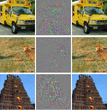
Adversarial examples (Szegedy et al., 2013).

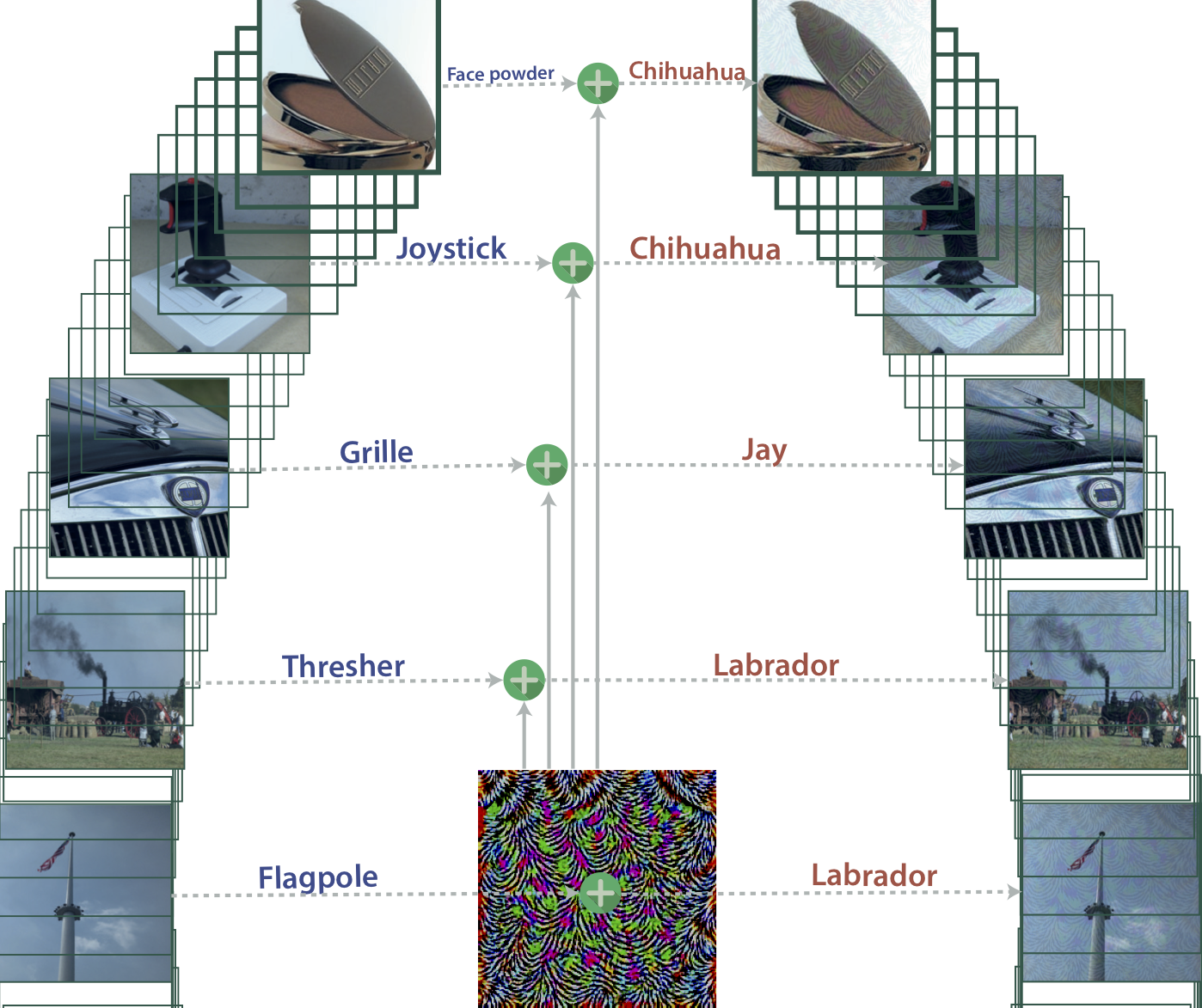
Universal Adversarial Perturbation (Moosavi-Dezfooli et al., 2017a).

Figure 2. An illustration of adversarial examples. (a) Specific perturbations for each new input. The images in the first column are inputs correctly classified, the ones in the middle are the perturbations used to induce a misclassification and the images on the last column (right) are the resulting adversarial examples. (b) Universal perturbations – only one perturbation can be applied to any picture on the left to generate adversarial examples on the right.

Optimization Attacks.

All attacks rely on optimization constructs. For example, in order to discover sensitive features, one can use the gradient taken w.r.t. one input. However, in this section we review the attacks that use optimization methods in order to search for solutions to eq. (LABEL:eq:adversarial_generic) or alternative forms and constraints.

Szegedy et al. (Szegedy et al., 2013) were the firsts to discover the DNNs sensitivity to adversarial examples and coin the term adversarial examples. The authors used limited memory box constrained optimization (L-BFGS) in order to approximate the minimum perturbation needed to change the label of an input, as in eq. (LABEL:eq:adversarial_generic). The initial experimental results showed that the minimum average distortion is very low, and can not be distinguished by human observers. This publication was the first to discover this behavior of DNNs and triggered a large array of publications.

Carlini and Wagner (Carlini and Wagner, 2017c) proposed an alternative form to eq. (LABEL:eq:adversarial_generic) in which the classification function is replaced due to its non-linear character. The alternative function is chosen s.t. $f({\bm{x}}+\eta)=\hat{y}$ if and only if $f({\bm{x}}+\eta)\leq 0$ (this is a linear constraint). This formulation allows the use of powerful optimization methods in order to search for very small perturbations and remains, at the time of writing this paper, one of the state-of-the-art attacks. Given its popularity, we will refer to this attack as the Carlini and Wagner attack.

The DeepFool attack (Moosavi Dezfooli et al., 2016) assumes DNNs behave linear around an input and projects the point to a separation plane between two classes. In the case of multi-class classifiers, the separation plane represents the face of a polyhedron whose faces are discriminants to other classes. The attack assumes the surface that separates two classes is defined by an implicit equation s.t. the geometrical normal is equal to its gradient vector.

Moosavi-Dezfooli et al.(Moosavi-Dezfooli et al., 2017a) use the DeepFool attack iteratively for all images in the training data set in order to find an universal perturbation – one that can be applied to any sample from the training set. An illustration of universal perturbation can be seen in Figure 2. Several passes over the training data set are required in order to improve the quality of the perturbation. At the end of the procedure, however, the method succeeds in finding image-agnostic perturbations which cause misclassifications with high confidence.

Although most publications consider adversarial examples in close resemblance to inputs drawn from the training set, Nguyen et al. (Nguyen et al., 2015) craft special images which can not be understood by human observers, but can generate a targeted classification with high accuracy. The authors leverage evolutionary algorithms in order to evolve candidate solutions that can fool DNNs. The fitness function evaluates candidates by sending the image to a target DNN.

Similarly, Su et al. (Su et al., 2019) use differential evolution – an evolutionary optimization method that ensures high population diversity – to generate adversarial perturbations. The output of the final softmax layer of a DNN is used as a fitness function for the algorithm; for targeted attacks the fitness function aims to increase the probability of a certain class, while for untargeted attacks it aims to decrease the probability of the true class. While it requires less information about the model under attack, this attack performs poorly when compared to gradient-based methods.

The attacks using the optimization strategy are generally precise in finding minimum perturbations or very good approximations of it. Although they are more complex than other types of attacks (because they require more iterations or use different optimization methods), most optimization based attacks are still state-of-the-art. From a security standpoint, an interesting approach is also to generate images that are not intelligible to humans, but can cause misclassifactions. This phenomenon links to several points in Section 9.

Sensitivity Analysis Attacks.

In order to overcome the speed drawbacks of the L-BFGS attack and following the linearity hypothesis introduced in the previous section, Goodfellow et al. (Goodfellow et al., 2015) proposed to sum small perturbations in the direction of the loss gradient taken w.r.t. one input. Moving a small step in the direction of the gradient results in taking a step towards maximizing the loss function. Analyzing the gradient of the loss function w.r.t. the input is often referred to as sensitivity or saliency analysis (Yeung et al., 2010) and reveals the importance of one feature in the decision process. Formally, the perturbation resulting from this simple attack (called Fast Gradient Sign (FGS)) is defined as: $\eta={\epsilon}\operatorname{sign}\left(\nabla_{\bm{x}}l({\bm{\theta}},{\bm{x}},y)\right)$. The value of $\epsilon$ controls the size of a perturbation and impacts the sensitivity of a human observer. Because this attack only requires the computation of the gradient vector, it is fast to apply and can be used to quickly generate new training data. However, this method trades precision for speed.

In order to increase the precision of FGS, Kurakin et al. (Kurakin et al., 2016b) propose to apply this method iteratively and, similar to the gradient clipping procedure, limit the value of a pixel by an upper bound. Moreover, the authors propose to use this method in a targeted fashion, by maximizing the likelihood for a chosen class. Madry et al. (Madry et al., 2018) extend the iterative attack proposed in (Kurakin et al., 2016b) by iteratively applying projected gradient descent (PGD) (Boyd and Vandenberghe, 2004) in order to search for a perturbation that can approximate the p-norm ball around an input. The use of PGD suggests the approximation is tractable and a large part of the loss landscape can be explored through it. If such a perturbation can be found and can approximate the entire p-norm ball, then protecting against it means one can protect against any perturbation in the norm ball.

Sharp curvatures near a data point can mask the true direction of steepest ascent and burden the discovery of adversarial examples with single-shot gradient methods (Kurakin et al., 2016a). In order to escape this phenomenon, Tramèr et al.(Tramèr et al., 2017a) introduce an attack that precedes single-shot attacks with a randomization step. Randomised Single Step Attack (RSSA) (Tramèr et al., 2017a) searches for an adversarial example starting every time from a random vicinity of the input data point, thus avoiding gradient masking (a phenomenon discussed in Section 7.4).

Dong et al. (Dong et al., 2018) proposed to boost the iterative version of FGS using gradient momentum. As in the case of gradient descent, momentum can stabilize the update directions and help escape poor local minimum/maxima by accumulating a velocity vector in the gradient direction. Setting the velocity vector to $0$ is equivalent to the normal FGS attack.

Papernot et al. (Papernot et al., 2016b) introduced an attack based solely on saliency analysis (Yeung et al., 2010). In order to discover the importance of each pixel in the decision process, a saliency map is generated by computing the forward derivative (forward Jacobian) of the function learned by a DNN. This method contrasts with early methods introduced in this section, which use the backward gradient of the loss function. The forward derivative allows to find better input feature, which ultimately lead to significant changes in the DNN output. However, its inherent computational costs for big images limits the impact of this method.

Similarly, Khrulkov and Oseledets (Khrulkov and Oseledets, 2018) used the Jacobian matrix to construct universal adversarial perturbations exploiting the singular value vectors of the feature maps while Huang et al. (Huang et al., 2015) use the Jacobian matrix to compute the linear approximation of a DNN output. The approximation for the normal and the perturbed case gives the minimal perturbation.

For cases when the gradient can not be well approximated – a phenomena called gradient masking and presented in Section 7.4 – Athalye et al. (Athalye et al., 2018a) introduced an attack which replaces the gradient of a non-differentiable layer with a differentiable approximation. Thus, the gradient of a DNN can be approximated by performing the forward pass through the whole network, but on the backward pass each layer is replaced by its approximation. As long as the two functions are similar, the slightly inaccurate gradients prove useful in constructing adversarial examples.

Chen et al. (Chen et al., 2018a) extrapolate the Carlini and Wagner attack (Carlini and Wagner, 2017c) from elastic-net regularization – a mixture of penalty functions used for high-dimensional feature selection.This algorithm is a bridge between optimization and sensitivity analysis methods because it uses different minimization techniques to discover sensitive features and, thus, adversarial examples.

The attacks based on sensitivity analysis are, generally, faster than the attacks based on the optimization strategy and can be more easily applied in training models with adversarial examples. In fact, training with an approximation of the p-norm ball around an input generated with PGD is one of the state-of-the-art defenses. However, these attacks are often less precise than the attacks based on the optimization strategy. Evaluating defenses against weak attacks might lead to a false sense of security, a topic we touch upon in Section 7.4.

Generative attacks.

Until now we introduced attacks that modify a sample from the data generating distribution by adding an adversarial perturbation. However, data samples might not always be available. In this section, we cover adversarial attacks based on generative models - a class of machine learning algorithms that learn to estimate a probability distribution by looking at samples drawn from it. The model is later used to produce artificial examples belonging to the same distribution. The goal is to generate examples that are similar to training samples, but not exactly the same. In particular, two generative models are used: (1) Variational Auto-Encoders (VAE) (Kingma and Welling, 2013; Rezende and Wierstra, 2014) and (2) Generative Adversarial Networks (GAN) (Goodfellow et al., 2014).

Baluja and Fischer (Baluja and Fischer, 2018) trained a DNN that transforms an input into an adversarial example. The transformation network is trained to fool a target network or to generate examples transferable to a larger range of networks. The authors use two approaches to generate adversarial examples: (1) using a residual network to generate a perturbation and (2) using auto-encoders. In practice, using auto-encoders yields better results and successfully scales to large data sets. The model is efficient to train, fast to execute, and produces diverse adversarial examples. Moreover, once the network is trained, the generation of adversarial examples only takes one step, suggesting its efficiency in adversarial training. However, this approach was not investigated.

Zhao et al. (Zhao et al., 2018a) search for adversarial examples in the deep representation of the input data (instead of searching directly in the input space). For this, a generator is trained to map random noise vectors to samples from the input distribution (from noise to input domain). A second generative model, called inverter, is trained to map data instances to corresponding dense representations (from input domain to noise). This is equivalent to finding an adversary in an underlying vector space which defines the data generation distribution and then map it back to the input space with the help of a generative model. However, the perturbations obtained through this method are far from the original inputs and can easily be spotted by human observers.

Poursaeed et al. (Poursaeed et al., 2018) trained a generative model to generate image dependent and independent perturbations; leading to specific or universal adversarial examples. However, in the universal case, the generator’s loss function is a linear combination of the loss functions of the target models, which makes it heavily dependent on the model under attack. Song et al. (Song et al., 2018b) used a generative model, similar to (Baluja and Fischer, 2018) against strong, certified defenses. Their results show that generative models can easily break defenses focusing on the p-norm ball, even though the defense guarantees no adversarial perturbation can be found in this region.

Generative models learn to approximate a distribution, from which we can sample new data. In the case of adversarial examples, generative models learn the distribution of perturbations, assuming that all perturbations are identically distributed. Although this assumption can be restrictive, even in this setting they are able to find powerful perturbations. However, training generative models often requires more resources and are rarely used in practical applications of adversarial examples.

6.1.2. Geometric Attacks

By now we have introduced algorithms that craft perturbations from noise. In this section, we review some attacks that use more natural, geometric transformations such as rotation or translation to construct adversarial examples.

Engstrom et al. (Engstrom et al., 2017) showed that only simple transformations - rotations and translations - are sufficient to create adversarial examples. These transformations are easy to craft and realistic in various operational scenarios. The authors propose several methods ranging from randomly sampling different transformations to grid search or gradient approaches. Depending on the chosen method, the drop in accuracy ranges from $34-90\%$ on models trained with data augmentation techniques (already including affine transformations).

ManiFool (Kanbak et al., 2018) searches for the smallest, worst-case, geometrical transformation that can fool DNNs. Similar to the perturbations generated by optimization or sensitivity based methods, these perturbations are imperceptible to human observers. The main idea behind ManiFool is simply to iteratively move from an image sample towards the decision boundary where the classification decision changes, while staying on the geometrical transformation manifold. In particular, the authors use a combination of rotation, translation and scaling transformations.

Xiao et al. (Xiao et al., 2018) proposed to change the geometry of the scene, while keeping the original appearance. Instead of imposing norm constraints on the pixel space, the authors introduce a new regularization loss on the local geometric distortion. The perceptual quality of the adversarial examples remains high, while most defenses fail against this attack. In a similar fashion, Zhang et al. (Zhang et al., 2019) change the geometry of the scene before applying the Carlini and Wagner attack. In this case, small transformations find inputs that are far away from the training data and lie in ’blind spots’ which are not covered by defenses. Once perturbed, these inputs lead to powerful attacks able to fool certified defenses. Although in this case the transformation is not the attack, it is an important preprocessing step which enables it.

Instead of using one transformation, Athalye et al. (Athalye et al., 2018b) search for perturbations over a distribution of transformations. In the 2D case, the authors use a random distribution of affine transformations, while in the 3D case they consider textures and shape. This technique is able to synthesize adversarial examples robust to defenses which use input transformations.

Pei et al. (Pei et al., 2017) proposed a framework for verifying the robustness of computer vision algorithms against natural perturbation such as rotation, translation or reflection (but also contrast, brightness or erosion). These adversarial examples are proved to be strong against state-of-the art classifiers, making the authors argue they are even stronger than gradient-based attacks. However, more evidence is needed to test this claim.

Geometrical transformations are thought to occur more frequently in the data acquisition process. However, most methods introduced in this section require carefully tuned transformations, which might limit this claim. Nonetheless, sensitivity to geometric transformations for models trained with data augmentation techniques shows that algorithms do not learn to abstract general transformations, but only to fit the training data.

6.2. Black box Attacks

The fact that adversarial examples generated for a model can transfer to others, regardless of architecture, was first observed by Szegedy et al. (Szegedy et al., 2013). However, this property was only later explored by Papernot et al. (Papernot et al., 2016a) in an attempt to evaluate black-box attacks. The authors examine how adversarial examples crafted on one model can transfer between several ML techniques such as linear regression, SVMs or DNNs. In such cases, an attacker has partial or full knowledge of the training data and can train a substitute model with it.

Later, Papernot et al. (Papernot et al., 2017) developed and evaluated practical black-box attacks against DNNs. In order to construct adversarial examples for a target model without any information available, the authors train a substitute model with data generated by the adversary and labeled by querying the target model. Afterwards, adversarial examples are crafted using attacks based on sensitivity analysis on the substitute model and transferred to the target model. In order to properly evaluate their technique, the authors attack various DNNs models hosted online by large companies and are able to generate misclassifications in most cases.

Liu et al. (Liu et al., 2016) generate adversarial examples for an ensemble of methods, hypothesizing that examples that transfer across several substitute models are more likely to transfer across a large array of black-box models. Their work is also the first attempt to scale black-box attacks on large data sets. Experimental results show that, in a targeted fashion, the precision of back-box attacks is quite low i.e. the adversarial examples do not maintain their intended class. However, if adversarial examples are used for untargeted black-box attacks, the success rate increases significantly.

Bhagoji et al. (Bhagoji et al., 2017) present an attack that removes the need to train substitute models. The authors approximate the gradient of a black-box model w.r.t. one input using the finite difference method and show its success by attacking pre-trained models or cloud deployed ones. Similarly, Chen et al. (Chen et al., 2017) present an attack called Zeroth Order optimisation (ZOO), that uses a derivative free optimization model. This method can estimate the gradient across the perturbation’s direction taking into consideration the value of the objective function at two neighboring points (corresponding to adding or subtracting a small perturbation). The experimental results show ZOO outperforms black box attacks that artificially train a substitute model (Papernot et al., 2017; Papernot et al., 2016a).

Another method that avoids training a substitute models was proposed by Narodytska and Kasiviswanathan (Narodytska and Kasiviswanathan, 2017). The authors use an iterative search procedure to explore the local neighborhood of a datapoint and refine the adversarial perturbation. This information provides an approximation of the gradient of the loss function w.r.t. to the input and, thus, provides valuable information about the sensitive pixels. Experimental results show good accuracy even for very deep networks. Other publications use genetic algorithms to synthesize adversarial examples (Alzantot et al., 2018) or to estimate the gradients (Ilyas et al., 2018) in order to generate adversarial examples in limited domains (such as limited queries or information). Outside image recognition, black-box adversarial examples have been used against malware detection systems (Rosenberg et al., 2017).

Black-box attacks rely on estimating the gradient’s direction and using it to generate perturbations. The applicability of substitute models is further discussed in Section 8, where the ability to transfer adversarial examples between different models is presented. Besides, other estimation techniques show good performance and have been tested with success in real life scenarios such as cloud ML service providers.

7. Defences

Similar to the attack evaluation introduced in Section 6, we provide a qualitative and a quantitative evaluation of each defense. The qualitative evaluation measures the performance of one defense against various attacks, its complexity and the testing setup, while the quantitative evaluation measures the literature impact. Each dimensions of both the qualitative and the quantitative assessment is measured on a categorical scale, ranging from low (*), medium(**) and high(***). The final score is computed by averaging over the attributes described below.

• Defense strength. The defense strength evaluates how powerful a defense is against different attacks (** or ***, depending on the attack’s strength) or if a defense was broken (*).

• Defense complexity. The defense complexity evaluates how easy it is to apply one defense (* if the defense is relatively easy to deploy, up to *** if the defense requires changing the model completely).

• Experimental setup. The experimental setup measures how thoroughly the defense was tested; if a threat model is presented (* if no, ** if the threat model is incomplete and *** if a correct threat model is presented), against which attacks is the defense tested (*, ** or ***, depending on the attack strength), and which data sets were used during evaluation (same as for attacks).

The quantitative evaluation is the same as for attacks: the ratio between the number of citations and the number of months since publication, as indicated by Google Scholar. Although bibliometrics are not a direct indicator of quality, they can be a good proxy to influential papers for a novice reader.

The results are presented together with the defense strategies discussed in Section 3.2 in Table 2. We note that the strongest defenses are the certified ones, although they also involve higher complexity. Whenever the perturbation space around a highly dimensional input can be well estimated, training with adversarial examples also leads to strong defenses (as in the case of Madry). Unfortunately the least complex defenses – i.e. guards – are also the least powerful. More details follow in the next sections. We conclude with a discussion the overall efficacy of the defenses (Section 7.3) and with a note on the evaluation of future defenses (Section 7.4).

7.1. Guards

Guards add a pre-processing step to the classification pipeline, in which adversarial examples are either detected or their impact is diminished by transforming the input. Because they do not alter the target model, guards have great potential.

Adversarial detectors are suited for tasks where refusing to process an input or discarding a classification is not mission critical. For example, an object detector from a cloud storage provider can refuse to classify one input, but an autonomous vehicle might not be able do so (since the input can be an important traffic sign). Moreover, based on the constructs used, adversarial detectors can also suffer from lack of robustness. Input transformations show great potential because they do not require any training and are easy to deploy. However, they can suffer from the same disadvantage as adversarial detectors because transforming an input might introduce other side effects. For example, compressing a high resolution medical image can lead to loss of accuracy.

7.1.1. Detection of Adversarial Examples.

Adversarial detectors use a variety of distinct features, as follows. Grosse et al. (Grosse et al., 2017) used a model agnostic statistical test to check if adversarial examples are outside the training data distribution. They observe that adversarial examples generated with some attacks can be found in different regions of the output surface than normal inputs and can be detected using statistical testing. Gong et al. (Gong et al., 2017) trained a separate DNN only with adversarial examples, able to successful detect adversarial examples with very small perturbations. Metzen et al. (Metzen et al., 2017) also trained a DNN for adversarial examples but, this time, the authors use the output of the DNN’s hidden layers. This techniques shows good result against weak attacks, but the detector’s performance diminishes agains iterative attacks. Similarly, Li and Li(Li and Li, 2017) developed an adversarial detector based on features extracted at every layer of a convolutional neural network. The authors treat an image as a distribution of pixels that can be used to collect statistics and used statistics from the hidden layers to train an adversarial detector.

Feinman et al. (Feinman et al., 2017) trained a linear detector using two distinct features: (1) the kernel density estimates in the subspace of the last layer and (2) the bayesian uncertainty estimates extracted from the drop-out layers (Gal and Ghahramani, 2016). They show that the bayesian uncertainty estimates are typically higher for adversarial examples, but not enough to successfully detect them. SafetyNet (Lu et al., 2017a) enforces an attacker to solve a discrete optimization problem. Each activation of a ReLU layer is quantized in order to generate a discrete code (assumed to be different for adversarial examples and normal inputs), later used to train an RBF-SVM adversarial detector with high accuracy.

Zhang et al. (Zhao et al., 2018b) proposed a new detection mechanism that hides the input labels from the adversary. This will prevent an attacker from maximizing the loss, given an input and a label and, thus, from creating an adversarial example. The authors define a one-to-one encoding scheme from true labels to code vectors. In order to detect adversarial examples, one can verify if the code vector computed from an input matches the signature of a class with certain precision. If the output is negative, the input is treated as an adversarial example. This approach shows good results on small data sets, but was not tested on more complex problems.

Abbasi and Gagné (Abbasi and Gagné, 2017) developed an ensemble of detectors based on the confusion matrix of each classifier. The underlying idea is that adversarial instances originating from a given class tend to fall into a small subset of incorrect classes. Therefore, developing an ensemble of detectors which can distinguish between confusion classes can more easily spot adversarial examples. However, this claim was only evaluated on toy networks and data sets. Meng and Chen (Meng and Chen, 2017) trained a model which distinguishes between a test and training input using the distance between an input and the data manifold. A thresholding function later decides if an input is normal or adversarial. However, the method is based on the existence of a distance function between an input and the data manifold.

Lee et al. (Lee et al., 2017) proposed a generative training method in which two DNNs are trained alternatively. The first network generates adversarial examples, while the second tries to correctly classify benign and adversarial examples. Similarly, Song et al. (Song et al., 2018a) used generative networks to purify adversarial examples and search for their true labels. The authors run, at first, a statistical test to detect if an input belongs to the data generation distribution and, if the test fails, recover the input using generative models. Ghosh et al. (Ghosh et al., 2018) designed a generative model that finds a latent random variable such that the input and its label become conditionally independent given the latent variable. The latent space is chosen as a mixture of Gaussians, such that each mixture component represents one of the classes in the data. Inferring the label given the latent encoding is done by computing the contribution of the mixture components. Adversarial samples are rejected based on thresholding the encoder and decoder outputs. For example, if the distance between the sample encoding and the encoding of the predicted class in the latent space is below a threshold.

Although a wide range of adversarial detectors have been developed, using very distinct features, many of them fail to detect strong, adaptive attacks. Moreover, their ability to generalize to new attacks is limited –  as new training is needed for new attacks – thus reducing their applicability.

7.1.2. Input Transformation.

Input transformations are thought to restrict the space of adversarial examples, therefore diminishing their impact. Guo et al. (Guo et al., 2018) suggest the use of several transformations: ”bit-depth reduction, JPEG compression, total variance minimization and image quilting” (Guo et al., 2018) as a pre-processing step to a convolutional classifier. The idea of using JPEG compression was also explored in (Dziugaite et al., 2016; Das et al., 2017; Shaham et al., 2018). Variance minimization and image quilting prove, in practice, the most effective transformations. Shaham et al. (Shaham et al., 2018) experiment with other input transformations: low-pass filters, PCA, low resolution wavelet approximations and soft-thresholding. They found all transformations provide some robustness against strong white and black box attacks. Xie et al. (Xie et al., 2018) propose to use two simple randomization operations: (1) random resizing of input images and (2) random padding with zeros around the input images. However, none of these approaches provide robustness against strong attacks.

Thermometer one hot encoding (Buckman et al., 2018) breaks the linear behavior of DNNs (suggested with the linearity hypothesis) by pre-processing the input with an extremely non-linear function. Instead of replacing a real number with its counterpart transformation, the authors replace each real number with a binary vector. Multiplying the input vector with the network’s weight enables different input values to use different parameters of the network. Inspired by thermometer encoding (Buckman et al., 2018), Rakin et al. (Rakin et al., 2018) proposed to process the input data using an ensemble of methods which includes the tanh function, batch normalization, thermometer encoding and one hot encoding. When used in combination with adversarial training, such methods show an increase in robustness because the resulting DNNs are less linear than normal ones. However, this increase is not powerful enough to protect against all adversarial examples.

Chen et al. (Chen et al., 2018b) proposed a pre-processing technique that can successfully mask the gradients, even for iterative attackers. Therefore, without access to the gradients, an attacker can not mount certain types of attacks. Their proposal is based on encoding the whole input space using a small set of separable codewords and training a classifier on the encoded information. Similarly, Liang et al. (Liang et al., 2017) treat perturbations as noise and use noise reduction methods in order to mitigate their threat. These methods show improvements for small data sets such as MNIST or CIFAR-10, but no improvements on larger data sets such as ImageNet.

In general, input transformations lead to stochastic gradients, which make attacks based on sensitivity analysis harder to mount. However, when tested against attacks using the optimization strategy, most input transformation defenses fail. We discuss this weakness in Section 7.4.

7.2. Defense by Design

This class of defenses alter the model, the data or the learning procedure in order to increase robustness. As opposed to guards, where some degree of robustness is achieved earlier in the processing pipeline, proactive defenses aim to design better architectures or training procedures.

7.2.1. Adversarial Traning.

Including adversarial examples in the training data set is a form of regularization (Girosi et al., 1995) i.e. a strategy designed to reduce the test error, possibly affecting the training error. Goodfellow et al. (Goodfellow et al., 2015) found that training with adversarial examples generated with the FGS attack, is an effective regularizer. However, because the attack is not strong, the training procedure does not increase robustness significantly. Sinha et al. (Sinha et al., 2018a) proposed a new training framework which assumes that simultaneous gradient updates should be statistically indistinguishable from each other. Thus, the gradient can be regularized in order to remove salient information, which can lead to adversarial examples. However, this phenomenon leads to masking the gradient and only protects against sensitivity analysis attacks. Lyu et al. (Lyu et al., 2015) abstracted from these a family of gradient based perturbations that can be used as regularization techniques. Their work is a generalization of the FGS-based training procedure for all possible norms. Roth et al. (Roth et al., 2018) proposed a similar method to regularize the gradients focused on the correlation structure of the perturbations. However, this method is data dependent and can only be used with certain types of perturbations.

Another way of training with adversarial examples is to completely exclude clean examples from the training procedure. This method is equivalent to training on the worst inputs possible, as in eq. (5). Solving the inner maximization problem increases the training time and might not always be tractable. In practice, however, approximating the result works very well.

Shaham et al. (Shaham et al., 2015) first investigated the min-max training procedure from eq. (5), but found the inner maximization problem intractable. Therefore, they propose to minimize an alternative form, in which they only evaluate a single step of the gradient (ascent and descent, corresponding to the steps in eq. (5)). Trying to solve the same problem, Huang et al. (Huang et al., 2015) use linear approximation to approximate the inner maximization problem. Madry et al. (Madry et al., 2018) use PGD for the inner maximization problem and suggest the problem is, in fact, tractable. In order to explore a large part of the loss landscape, PGD is restarted from many points in the ball around an input. Surprisingly, although there are many local maxima spread widely apart within this space, they tend to have very well concentrated loss values. This suggests that an adversarial example found by this method is representative for all adversarial examples generated with first order methods.

Tramèr et al. (Tramèr et al., 2017a) developed a technique that augments training data with adversarial examples crafted on other static, pre-trained, models. Training with ensemble methods increases the diversity of perturbations seen during training. This is equivalent to enhancing the uncertainty sets with examples crafted on other models. Dhillon et al. (Dhillon et al., 2018) define a min-max zero-sum game between an adversary and a DNN. The strategy for this game is to prune a random subset of activations (e.g. those with smaller magnitude) and scale-up the survivors in order to compensate. This approach is similar to the dropout technique, where the activations with high absolute values have a higher chance of being sampled.

In practice, adversarial training with the worse case perturbation yields very good results. The Madry (Madry et al., 2018) training procedure, which approximates the inner maximization problem using PGD is a state-of-the-art defense. Finding new and faster approximation methods was not explored in depth and remains an open question.

7.2.2. Architectural Defenses.

Some defenses propose to change the model’s architecture by either imposing layer-wise constraints or by altering the final layer. One of the first proposals uses distillation – a transfer learning method in which smaller DNNs are trained with knowledge extracted from larger DNNs (Hinton et al., 2015). Papernot et al. (Papernot et al., 2016c) used distillation in order to increase the DNNs robustness. However, instead of using multiple DNNs in the training process, distillation is used for a single DNN. As opposed to the original distillation mechanism, the same network architecture is used both for training and distillation. Cisse et al. (Cisse et al., 2017) introduced a regularization scheme that constrains the Lipschitz constant layer-wise, thus avoiding any exponential growth of the constant. In this setting, a regularization scheme (such as weight decay) applied to the last layer controls the overall Lipschitz constant of the network.

Similarly, Gu and Rigazio (Gu and Rigazio, 2014) proposed a new network architecture, called deep contractive networks, which imposes a layer-wise constraint. This constraint minimizes the network’s output variance w.r.t. perturbations in the input s.t. a trained model can achieve robustness for perturbations around training data points. Nayebi and Ganguli (Nayebi and Ganguli, 2017) developed a new training scheme inspired by biophysical principles in neural circuits. Following the idea suggested by Goodfellow et al. (Goodfellow et al., 2015) that adversarial examples are due to the linear summing of high dimensional input with small weights, the authors propose to force neural networks to operate in a non-linear, saturated, regime. In order to enforce this constraint, the authors ensure that each element of the Jacobian matrix of the model is sufficiently small s.t. the model becomes insensitive to perturbations.

DeepCloak (Gao et al., 2017) removes features not used in classification in order to increase robustness to adversarial examples. To identify unnecessary features, adversarial samples are tested against the clean example. In order to remove the features, a mask layer is introduced before the logits layer. The mask serves as a selector, keeping the necessary features and setting the unnecessary to null. Lamb et al. (Lamb et al., 2018) identify which hidden states are off the data manifold and map these states back to parts of the data manifold where the network performs better. This process consists of inserting de-noising auto-encoders at crucial points between layers of the original network in order to clean up the transformed data points which may lie outside the data manifold. Dumont et al. (Dumont et al., 2018) investigated the resistance to adversarial attacks of three rotation-equivariant network architectures (Cohen and Welling, 2016). They discover that rotation equivariant networks are significantly more robust to attacks based on small translations and rotations, but marginally robust against attacks based on local geometric distortions.

Sun et al. (Sun et al., 2017) proposed to use data dependent weights for each hidden layers of DNNs. The weights are generated using HyperNetworks (Ha et al., 2017) – a training technique in which a DNN generates the weights for another. The weights create an inductive bias specific to the training set which alleviates the effect of adversarial examples for small perturbations. Pontes-Filho and Liwicki (Pontes-Filho and Liwicki, 2018) proposed to use bidirectional learning in order to increase robustness to adversarial examples. Bidirectional learning trains two models – the first on the inputs and the second on a reversed copy of the inputs. However, in (Pontes-Filho and Liwicki, 2018), a single model is trained to behave both as a discriminative and generative model. Therefore, the same model can be a classifier and a generator in the same time. This behavior is achieved using an un-directed DNN that back-propagates the errors in both directions – each direction of the network has its own biases and the weights are shared.

Dense associative models (Krotov and Hopfield, 2016) store a set of vectors in memory, corresponding to the learnt patterns. For example, pixel characteristics (such as intensity) can be stored together with the corresponding label. At query time, the model tries to recover the memory sequences from incomplete data (corresponding to variations of an input, or perturbations). If strong perturbations are applied to an input, the model will fail to recover the original label and consider the input adversarial.

Given the linear conjecture, introduced in Section 5, which states that adversarial examples exploit the linear behavior of DNNs, a normal attempt to increase robustness is to use more non-linear activation functions. Goodfellow et al. (Goodfellow et al., 2015) suggested that RBF networks – which behave in a non-linear manner – are naturally immune to adversarial examples and have low confidence when they are fooled. However, RBF units can not generalize very well and do not achieve the same performance as ReLU based DNNs. Krotov and Hopfield (Krotov and Hopfield, 2017) tried to replace ReLU activations with higher rectified polynomials and observed an increase in robustness. However, the increase is not sufficient to completely remove the adversarial phenomenon.

Several publications suggested that DNNs capacity increases their robustness to adversarial examples(Madry et al., 2018; Kurakin et al., 2016b; Rozsa et al., 2016a). However, this correlation was not further investigated .

7.2.3. Certified Defenses

Certified defenses rely on formal verification techniques in order to guarantee that robustness holds within the bounds defined in Section 4,for the training data set. Certified defenses can be broadly classified based on the guarantees they give in (1) exact, deterministic guarantees –  which give a proof of robustness, (2) one-sided guarantees – which find a lower or an upper bound for robustness, (3) converging lower or upper bound or (4) statistical guarantees, which quantify the probability that a model is robust (Huang et al., 2018).

Proving deterministic guarantees for robustness has been formulated as a constrained solving problem where solutions are searched using SMT or mixed integer solvers. Two approaches, namely Reluplex (Katz et al., 2017) and Planet (Ehlers, 2017), use SMT solvers to verify robustness constraints for DNNs with ReLU activations. Reluplex adapts the Simplex algorithm with rules for non-convex optimization in order to handle ReLU function, while Planet uses linear approximation in order to over-approximate the network’s behavior. If a property is not satisfied, these algorithms return counterexamples, which constitutes valid adversarial examples. Carlini et al. (Carlini et al., 2018) extends Reluplex to verify $p_{1}$ and $p_{\infty}$ norm adversarial examples by encoding absolute values using ReLUs. Scaling SMT/SAT solvers for larger models is, however, difficult and remains an open issue.

Other approaches have focused on certifying lower or upper bounds on the existence of adversarial examples. Wong and Kolter (Wong and Kolter, 2018) consider a convex outer approximation of the set of activation values which can be reached using adversarial examples and use linear programming to minimize the loss in this region. The dual of the linear program can be specified as a DNN, making the process efficient. Dvijotham et al. (Dvijotham et al., 2018) propose a similar form in which the dual problem is formulated and solved using a Lagragian relaxation of the optimization problem, thus obtaining an upper bound on the robustness against adversarial examples. A different method to certify lower or upper bounds is to encode the inputs in an abstract domain, which contains all perturbations (e.g. a zonotope), and train with it (Mirman et al., 2018; Gehr et al., 2018; Yang et al., 2019). Similarly, Gowal et al. (Gowal et al., 2018) use interval bound propagation for training verifiable robust models. These approaches are very effective and can scale to larger models.

Huang et al. (Huang et al., 2017a) give proofs of convergence using SMT solvers by exhaustively searching for perturbations in a given norm ball, at each layer of DNNs. Later, Wicker et al. (Wicker et al., 2018) and Wu et al. (Wu et al., 2018) extend the search using Monte-Carlo tree search methods. The publications discussed in Section 4, however, give statistical guarantees to robustness (Bastani et al., 2016; Weng et al., 2018; Ruan et al., 2018).

Through their ability to guarantee that perturbations within some bounds can not cause misclassifications, certified defenses are well suited for tasks where robustness is paramount. However, some techniques (such as using SMT solvers) are very complex, require more training resources and often do not scale to deep models. Therefore, their applicability is reduced. Moreover, guarantees can be given only for the training data set. As discussed in the following section, there are attacks which can bypass these defenses.

7.3. On the Overall Efficacy of Adversarial Defenses

One limitation of most publications presented in the previous sections is the lack of rigorous evaluation. With the exception of defenses that guarantee robustness within some bounds, other publications do not provide sufficient evidence for their effectiveness. Therefore, the efficacy of these defenses is often over-emphasized. Fortunately, some publications questioned their success and showed some defenses are, in fact, not effective.

Carlini and Wagner (Carlini and Wagner, 2017a) evaluated the efficacy of adversarial detection methods and proved that most detectors perform poorly when faced with strong, iterative, attacks. In particular, the authors use the Carlini and Wagner attack (Carlini and Wagner, 2017c) to show that none of the detectors – (Bhagoji et al., 2018; Feinman et al., 2017; Gong et al., 2017; Grosse et al., 2017; Hendrycks and Gimpel, 2016; Metzen et al., 2017; Li and Li, 2017) – efficiently detect adversarial examples and that their reported results do not reflect the reality. Moreover, Athalye et al. (Athalye et al., 2018b) broke the (Lu et al., 2017b) detector. In another paper, Carlini and Wagner (Carlini and Wagner, 2017b) show that MagNet (Meng and Chen, 2017) is also easily defeated by adaptive attacks.

Conversely, Athalye et al. (Athalye et al., 2018a) showed that 7 out of 9 defenses published at ICLR 2018 as non-certified defenses suffer from gradient masking (a phenomenon described in the next section) and are not efficient against the BPDA attack (Table 1). Although the other 2 defenses do not suffer from gradient masking, they have also been broken. He et al. (He et al., 2017) show that combining adversarial defenses in an ensemble defense is also not effective, while Sharma and Chen (Sharma and Chen, 2017) broke the adversary training method based on the Madry attack (Madry et al., 2018). Moreover, certified defenses can be bypassed using generative models (Poursaeed et al., 2018) or with perturbations outside the pixel norm ball (Liu et al., 2018b). Zhang et al. (Zhang et al., 2019) showed that robust adversarial training and certified defenses only protect in regions close to the training data, but fail to protect against inputs away from these regions.

Given these results, the overall efficacy of all adversarial defenses is under scrutiny. A protocol for defense evaluation is presented in the following section.

7.4. Gradient Masking and Defense Evaluation

Many defenses alleviate the model’s sensitivity to small changes in the input by minimizing the gradients during the learning phase or constructing models without useful gradients. However, forbidding access to gradient information is not enough to limit an attacker from constructing adversarial examples (Papernot et al., 2017). This phenomenon, called gradient masking (Papernot et al., 2018, 2017) was identified to give a false sense of security and leads to an improper evaluation of adversarial defenses (Athalye et al., 2018a; Tramèr et al., 2017a; Carlini and Wagner, 2017a). For example, Galloway et al. (Galloway et al., 2017) found that binarized neural networks exhibit stronger gradient masking, which sometimes gives them an advantage over full precision models, however, these methods only provide apparent robustness. Defenses that exploit gradient masking can be sometimes broken with stronger attacks (Carlini and Wagner, 2017a; Carlini et al., 2019).

Moreover, applying a defense may lead to a false sense of security because current defenses imply an attacker does not know the defense is used. The subject of correctly evaluating adversarial defenses is at the forefront of research in adversarial examples and has proven to be not trivial (Carlini et al., 2019). Carlini et al. (Carlini et al., 2019) provide a methodological foundation for evaluating adversarial defenses. Their suggestions are based on skepticism of the results and evaluation against strong, adaptive, attacks: the attack models should include the possible defense mechanisms employed. Therefore, the evaluation must include the budget an attacker needs to spend in order to break a defense she knows. At this moment, their work suggest the best protocol for evaluating new defenses and should be considered whenever a new defense is designed.

8. Transferability

Besides the existence of adversarial examples, Szegedy et al. (Szegedy et al., 2013) showed that adversarial examples can transfer between different ML models. This phenomenon was later explored by Papernot et al. (Papernot et al., 2016a), who studied the ability to transfer adversarial examples not only between DNNs, but also between different ML techniques. The authors identified two types of transferable adversarial examples: (1) intra-technique examples – which transfer between models trained with the same ML method and (2) cross-technique examples – which transfer between models using different methods. Papernot et al. found that all ML models are vulnerable to intra-technique adversarial examples. The phenomenon shows stronger for differentiable models than for non-differentiable models. In regard to cross-technique adversarial examples, linear models, SVMs, decision trees or ensembles of models are more vulnerable between themselves compared to DNNs, which maintain some resilience against such techniques. Later, Demontis et al. (Demontis et al., 2019) showed that transferability is dependent on the input gradient’s size (for the target classifier) and on the loss variance for the base base classifier. Less complex or regularized models, which lead to smaller input gradients, tend to be more robust.

Liu et al. (Liu et al., 2016) investigated the transferability phenomenon at larger scale, using the ImageNet data set and various DNNs architectures. Moreover, the authors discuss transferability in close relation to the attacker’s goals (Section 3.1): (1) to cause an untargeted or (2) a targeted misclassification. The experimental results show untargeted attacks transfer easily intra-technique. In contrast, targeted attacks do not maintain labels during transfer. Moreover, when only the hyper-parameters vary (but the architecture is preserved), transferability is not consistent, revealing that transferability depends on hyper-parameters. The results are strengthened by Su et al. (Su et al., 2018) who run a large scale study of transferability between different DNN architectures and show that targeted adversarial examples do not transfer between architectures. However, transferability can be used to reverse engineer models and find the base architecture.

Tramèr et al. (Tramèr et al., 2017b) show empirical evidence that different models draw similar decision boundaries and proposed a method to measure the space where adversarial examples can be found. Following the hypothesis that adversarial examples inhabit large, continuous regions instead of small pockets of the manifold (Section 5), the authors measure the number of orthogonal perturbations that can lead to misclassifications. Although these vectors are not sufficient to represent a basis of the adversarial space, they are a good indicator of its size. Experimental results show this number depends on the network architecture. Nonetheless, even small adversarial spaces are sufficient to intersect across different models and give transferable examples. This study also shows that transferability is inherent to models which learn feature spaces with non-robust properties in the input space; an idea further developed in (Ilyas et al., 2019). If models were to learn (or designed to select) distinct features with robust properties in the input space, it would be impossible to transfer adversarial examples. Therefore, transferability emerges as a consequence of algorithm design.

In summary, the literature brings empirical evidence to show that different ML algorithms learn a close representation of the input space. Therefore, evading a region corresponding to a correct class with sufficient distance from the boundaries would most certainly transfer between models. However, while the representation of classes is similar, they are not distributed alike in the output space, making it harder to transfer an input in a desired target region.

9. Discussion

The literature on adversarial examples makes different claims about their impact on security and safety, although in practice all publications use the definition of robustness from Section 4 as a proxy to either of these notions. In this section we discuss the relevance of robustness to security and safety and the economics of building more robust models. Moreover, since p-norm is the dominant similarity metric, we also comment on its relevance. This section ends with a discussion on the representations learned by DNNs and how they impact adversarial examples.

On the relevance of robustness to security.

Gilmer et al. (Gilmer et al., 2018a) express some skepticism about whether adversarial examples are always a serious security concern. Here it is interesting to note again that much of the early work on adversarial machine learning (Lowd and Meek, 2005; Barreno et al., 2010) concerned applications of ML for security tasks, such as detecting spam, malware, or network intrusions. In such applications there is by definition an attacker interested in causing misclassification, as the whole point of the system is to defend against such an attacker, and hence misclassifications - esp. false negatives – clearly have a security impact. By contrast, most recent work on adversarial learning focuses on computer vision. While adversarial examples may seem worrying thinking of some applications of computer vision, say automated driving, this does not imply that there is an interesting way for attackers to exploit it. For example, Eykholt et al. (Eykholt et al., 2018) use perturbed stop signs to attack autonomous vehicles. However, the perturbations are far from sensible and can be detected by human observers. Simply obscuring or removing the stop sign or may be easier ways to achieve the same effect.

Since adversarial examples rely on small perturbations, which can not be distinguished by human observers, they seem to be appropriate for attacks on systems which interact with humans or when the content of the message should not be heavily modified. However, until now there are not many scenarios in which the lack of robustness defined as in Section 4 has strong security consequences. Searching for attacks which can only be mounted with adversarial examples against systems that do not carry out security tasks is important to assess their real impact on security.

On the relevance of robustness to safety.

From an engineering perspective, safety is the ability of a system to protect its users from harmful or non-desirable outcomes. The distinction between security and safety is that security protects a system against intentional, malicious, attacks while safety protects a system from unintended mishaps in the operational environment. Some publications aim to improve or validate the safety of DNNs – e.g. (Huang et al., 2017a; Lu et al., 2017a; Gehr et al., 2018). However, safety is an inherent property of a system and not of an algorithm solely. Moreover, safety becomes important when a system can produce physical or material damage to humans, assets or the environment. Talking about safety for systems without such impact – e.g. an image based search engine using ML – is futile. In order to guarantee safety, one should make sure that possible errors are detected and contained inside the system without affecting its normal operation. Take again the example of an autonomous vehicle. If the outcome of its computer vision system is cross checked with information coming from maps, the effect of using adversarial examples on traffic signs can be detected and contained inside the system, reducing their impact on safety.

The discussion of ML safety in relation to the robustness definition from Section 4 should take into account the operational environment of an algorithm because some perturbations (such as those needed to build adversarial examples) may never appear in some environments, but may be common in others. Besides, it might also be interesting to benchmark an algorithm and increase its robustness to common corruptions and perturbations (Hendrycks and Dietterich, 2019). Following this direction may reveal spots where current algorithms fail although the operational settings are natural and can be more relevant for safety. Moreover, searching for distance metrics to better reflect the uncertainties in the operational environment of a system may lead to new threats to safety.

On the relevance of p-norm.

The dominant similarity metric in the literature is the p-norm distance defined in Section 2. Choosing an adequate metric is still an open question. However, since there are no solutions to robustness for the p-norm distance, it is hard to believe that using other metrics will result in more robust models (Carlini et al., 2019). Nonetheless, there is an increased interest to explore new distance functions, e.g. the Wasserstein distance (Wong et al., 2019) or using physical parameters underlying the image formation process (Liu et al., 2018b). This is an interesting direction to pursue, which may lead to new attack and defense strategies and new insights about ML algorithms. We argue that the p-norm remains relevant for experimental settings; however, it must be paired with relevant threat models in order to evaluate its impact in security and search for operational environments where it impacts safety. Exploring new metrics and scenarios in which lack of robustness poses threats to safety or security is an important direction for future research.

On the economics of defending against adversarial examples.

Until now there seems to be a tradeoff between accuracy and robustness to adversarial examples, inherent to the algorithms and the training methods used. Moreover, the results presented in Section 5 suggest that training models robust to adversarial examples requires more resources than non-robust ones. This means robustness comes at a cost. Whether these cost are acceptable, and how high they can be, will depend on the application and the context. Given that ML systems are not widely deployed and, as mentioned earlier, the real impact of adversarial examples on safety and security is still to be determined, it remains to be seen which defenses can be cost-effective in practice.

On the representations learned by DNNs.

The sensitivity of DNNs to adversarial examples raises questions about their ability to learn high level abstractions from data. Although it is believed that increasing the depth of a network helps increasing the level of abstraction and it was observed that early layers in convolutional networks learn filters that resemble contour extractors, while deeper layers learn more complex patterns, DNNs seem to learn superficial abstractions restricted to the space on which they operate. In object recognition, the training objectives lie in pixel space, and not in a conceptual or relational space. Pixel spaces are necessary for extracting first order information about the task, but seem to be insufficient for higher level abstractions needed to overcome complex perception systems. Moreover, the capacity to create adversarial inputs which are not intelligible by humans (as in (Nguyen et al., 2015)) shows that DNNs use different features than we wish for. Research in adversarial examples strengthen the conclusions from Jo and Bengio (Jo and Bengio, 2017) which analyzed convolutional networks in different regimes and showed they exhibit a tendency to learn surface regularities rather than higher-level abstract concepts. Therefore, adversarial examples might be intrinsic to the methods used to solve ML related tasks or to the current training procedures. In this context, it is interesting to search for models which learn a better representation of the world and which may solve the sensitivity to adversarial examples as a side effect.

10. Conclusions and Future Research

We focused on several aspects of the adversarial examples phenomenon, in an attempt to provide a comprehensive and self contained survey of this field of research. In particular, we focused on explaining the hypotheses on the existence of adversarial examples, position the phenomenon in the security and robustness context, describe and characterize the attacks and defenses proposed in the literature and present the ability of adversarial examples to transfer between different ML techniques. In the appendix we have included examples of software libraries and competitions for developing attacks and defenses.

To conclude, we note that adversarial examples are an intriguing phenomenon of ML algorithms and their existence can raise both safety or security alarms. However, their true impact on safety and securiity is hard to estimate at this moment in time. A key take away is that the phenomenon of adversarial examples has no generally accepted explanation or solution. Moreover, until now all defenses (including the ones using formal verification) have been broken. Therefore, the field remains active and spans several future research directions.

At first, since no universally accepted conjecture on the existence of adversarial examples exist, a more fundamental approach is required. Such an inquiry can use methods from topology (to analyze the data manifold or the decision boundaries), from statistics (to extract information about distribution of adversarial examples) or from learning theory (to investigate in which theoretical settings the resources needed for training robust models can be decreased). Nonetheless, such an inquiry must be accompanied by practical reasoning about the impact of adversarial examples on security by developing, for example, new threat models. Similarly for safety, by searching for operational scenarios in which the deployment of ML algorithms is hindered by adversarial examples or searching for scenarios that require new ways to measure and certify robustness.

Secondly, the use of certified defenses suggests robustness within certain bounds can be achieved (or, at least, precisely measured). It is interesting to search for new certified defenses with small computational complexity, which can better scale to large models. When designing new certified defenses it is important to consider how new techniques can help increase the bounds for robustness and not only precisely measure it. Moreover, in ideal settings, new defenses should alter the models as little as possible and should help already trained models too. Besides, it is important to search for spaces where certify defenses fail or investigate attacks which can break them. At the moment, this research is sparse, giving some indications that certified defenses can also be bypassed (Poursaeed et al., 2018).

Thirdly, although asymptotic results suggest solving the adversarial examples problem requires more resources (data or computational), searching for new approximate solutions is essential. For other tasks, theoretical results suggest similar limits, although approximate solutions already achieve very good results. Therefore, finding better methods to approximate the perturbation space and train robust models in low data regimes is an interesting research direction.

Lastly, one important take away from analyzing the phenomenon of adversarial examples is that ML and, in particular, DNNs operate in spaces less abstract than humans do. Therefore, perturbations with no impact in the human space have a large impact in the algorithmic space. We may compare adversarial examples with human optical illusions, where one is fooled by perceiving individual stimuli as a whole or illusions that create images different from the objects that make them (e.g. the rabbit-duck illusion). These subjective stances humans experience, called qualia, have been long studied in philosophy and psychology and are common in the space of human cognition or emotion. However, human beings are able to identify when such phenomenons occur (most humans can identify an optical illusion as an optical illusion, but can not classify its content correctly). Moreover, the effect of illusions or subjective beliefs can be removed by humans through rational analysis. This type of analysis has been identified as using the ’slower’ part of our cognition system, which seems to be missing from the way ML models are currently built. If limited by time, humans can also be fooled by adversarial examples (Elsayed et al., 2018). However, our capacity to engage in rational analysis and adapt to the environment removes such threats and remains to be implemented in machines.

Appendix A Tools and Competitions

The libraries from Table 4 implement some of the attacks and defenses presented in this paper. Moreover, there is an increasing number of competitions for developing new attacks and defense, some of which are mentioned in Table 4.

Name	Link
CleverHans	https://cleverhans.readthedocs.io
Foolbox	https://foolbox.readthedocs.io
Adversarial Toolbox	https://adversarial-robustness-toolbox.readthedocs.io/
Advertorch	https://github.com/BorealisAI/advertorch

Table 3. List of libraries for attacks and defenses.

Name	Link
Unrestricted Adv. Examples	https://tinyurl.com/y3xrgoy2
Adv. Vision Challenge	https://tinyurl.com/y5hhwomk
CAAD	https://tinyurl.com/rrk7e78

Table 4. List of adversarial competitions.

References

- (1)
- Abbasi and Gagné (2017) Mahdieh Abbasi and Christian Gagné. 2017. Robustness to adversarial examples through an ensemble of specialists. arXiv:1702.06856.
- Akhtar and Mian (2018) Naveed Akhtar and Ajmal Mian. 2018. Threat of adversarial attacks on deep learning in computer vision: A survey. IEEE Access (2018).
- Alzantot et al. (2018) Moustafa Alzantot, Yash Sharma, Supriyo Chakraborty, and Mani Srivastava. 2018. GenAttack: Practical Black-box Attacks with Gradient-Free Optimization. arXiv:1805.11090.
- Athalye et al. (2018a) Anish Athalye, Nicholas Carlini, and David Wagner. 2018a. Obfuscated gradients give a false sense of security: Circumventing defenses to adversarial examples. ICML (2018).
- Athalye et al. (2018b) Anish Athalye, Logan Engstrom, Andrew Ilyas, and Kevin Kwok. 2018b. Synthesizing robust adversarial examples. ICML (2018).
- Baluja and Fischer (2018) Shumeet Baluja and Ian Fischer. 2018. Adversarial transformation networks: Learning to generate adversarial examples. In AAAI.
- Barreno et al. (2010) Marco Barreno, Blaine Nelson, Anthony D. Joseph, and JD. Tygar. 2010. The security of machine learning. Machine Learning (2010).
- Barreno et al. (2006) Marco Barreno, Blaine Nelson, Russell Sears, Anthony D. Joseph, and J. Doug Tygar. 2006. Can machine learning be secure?. In ASIACCS. ACM.
- Bastani et al. (2016) Osbert Bastani, Yani Ioannou, Leonidas Lampropoulos, Dimitrios Vytiniotis, Aditya Nori, and Antonio Criminisi. 2016. Measuring neural net robustness with constraints. NeurIPS (2016).
- Behzadan and Munir (2017) Vahid Behzadan and Arslan Munir. 2017. Vulnerability of deep reinforcement learning to policy induction attacks. In Int. Conference on Machine Learning and Data Mining in Pattern Recognition. Springer.
- Ben-Tal et al. (2009) Aharon Ben-Tal, Laurent El Ghaoui, and Arkadi Nemirovski. 2009. Robust optimization. Princeton University Press.
- Bhagoji et al. (2018) Arjun Nitin Bhagoji, Daniel Cullina, Chawin Sitawarin, and Prateek Mittal. 2018. Enhancing robustness of machine learning systems via data transformations. In CISS. IEEE.
- Bhagoji et al. (2017) Arjun Nitin Bhagoji, Warren He, Bo Li, and Dawn Song. 2017. Exploring the Space of Black-box Attacks on Deep Neural Networks. arXiv:1712.09491.
- Biggio et al. (2014) Battista Biggio, Giorgio Fumera, and Fabio Roli. 2014. Security evaluation of pattern classifiers under attack. In TKDE. IEEE.
- Biggio et al. (2012) Battista Biggio, Blaine Nelson, and Pavel Laskov. 2012. Poisoning attacks against support vector machines. arXiv:1206.6389.
- Biggio and Roli (2018) Battista Biggio and Fabio Roli. 2018. Wild patterns: Ten years after the rise of adversarial machine learning. Pattern Recognition (2018).
- Boyd and Vandenberghe (2004) Stephen Boyd and Lieven Vandenberghe. 2004. Convex optimization. Cambridge University Press.
- Brückner et al. (2012) Michael Brückner, Christian Kanzow, and Tobias Scheffer. 2012. Static prediction games for adversarial learning problems. JMLR (2012).
- Bubeck et al. (2018) Sébastien Bubeck, Eric Price, and Ilya Razenshteyn. 2018. Adversarial examples from computational constraints. arXiv:1805.10204.
- Buckman et al. (2018) Jacob Buckman, Aurko Roy, Colin Raffel, and Ian Goodfellow. 2018. Thermometer encoding: One hot way to resist adversarial examples. ICLR (2018).
- Carlini et al. (2019) Nicholas Carlini, Anish Athalye, Nicolas Papernot, Wieland Brendel, Jonas Rauber, Dimitris Tsipras, Ian J. Goodfellow, Aleksander Madry, and Alexey Kurakin. 2019. On Evaluating Adversarial Robustness. arXiv:1902.06705 (2019).
- Carlini et al. (2018) Nicholas Carlini, Guy Katz, Clark Berret, and David Dill. 2018. Provably Minimally-Distorted Adversarial Examples. arXiv:1711.00851.
- Carlini et al. (2016) Nicholas Carlini, Pratyush Mishra, Tavish Vaidya, Yuankai Zhang, Micah Sherr, Clay Shields, David Wagner, and Wenchao Zhou. 2016. Hidden Voice Commands. In USENIX Security.
- Carlini and Wagner (2017a) Nicholas Carlini and David Wagner. 2017a. Adversarial examples are not easily detected: Bypassing ten detection methods. In AISec. ACM.
- Carlini and Wagner (2017b) Nicholas Carlini and David Wagner. 2017b. Magnet and ”Efficient defenses against adversarial attacks” are not robust to adversarial examples. arXiv:1711.08478.
- Carlini and Wagner (2017c) Nicholas Carlini and David Wagner. 2017c. Towards evaluating the robustness of neural networks. In S&P. IEEE.
- Carlini and Wagner (2018) Nicholas Carlini and David Wagner. 2018. Audio adversarial examples: Targeted attacks on speech-to-text. arXiv:1801.01944.
- Chen et al. (2018b) Jiefeng Chen, Xi Wu, Yingyu Liang, and Somesh Jha. 2018b. Improving Adversarial Robustness by Data-Specific Discretization. arXiv:1805.07816.
- Chen et al. (2018a) Pin-Yu Chen, Yash Sharma, Huan Zhang, Jinfeng Yi, and Cho-Jui Hsieh. 2018a. EAD: elastic-net attacks to deep neural networks via adversarial examples. In AAAI.
- Chen et al. (2017) Pin-Yu Chen, Huan Zhang, Yash Sharma, Jinfeng Yi, and Cho-Jui Hsieh. 2017. ZOO: Zeroth order optimization based black-box attacks to deep neural networks without training substitute models. In AISec. ACM.
- Cisse et al. (2017) Moustapha Cisse, Piotr Bojanowski, Edouard Grave, Yann Dauphin, and Nicolas Usunier. 2017. Parseval networks: Improving robustness to adversarial examples. ICML (2017).
- Cohen and Welling (2016) Taco Cohen and Max Welling. 2016. Group equivariant convolutional networks. ICML (2016).
- Cullina et al. (2018) Daniel Cullina, Arjun Nitin Bhagoji, and Prateek Mittal. 2018. PAC-learning in the presence of evasion adversaries. arXiv:1806.01471.
- Dalvi et al. (2004) Nilesh Dalvi, Pedro Domingos, Sumit Sanghai, Deepak Verma, et al. 2004. Adversarial classification. In SIGKDD. ACM.
- Das et al. (2017) Nilaksh Das, Madhuri Shanbhogue, Shang-Tse Chen, Fred Hohman, Li Chen, Michael E. Kounavis, and Duen Horng Chau. 2017. Keeping the bad guys out: Protecting and vaccinating deep learning with JPEG compression. arXiv:1705.02900.
- Demontis et al. (2019) Ambra Demontis, Marco Melis, Maura Pintor, Matthew Jagielski, Battista Biggio, Alina Oprea, Cristina Nita-Rotaru, and Fabio Roli. 2019. Why do adversarial attacks transfer? explaining transferability of evasion and poisoning attacks. In USENIX Security.
- Demontis et al. (2016) Ambra Demontis, Paolo Russu, Battista Biggio, Giorgio Fumera, and Fabio Roli. 2016. On security and sparsity of linear classifiers for adversarial settings. In Int. Workshops on SPR and SSPR. Springer.
- Dhillon et al. (2018) Guneet S. Dhillon, Kamyar Azizzadenesheli, Zachary C. Lipton, Jeremy Bernstein, Jean Kossaifi, Aran Khanna, and Anima Anandkumar. 2018. Stochastic activation pruning for robust adversarial defense. arXiv:1803.01442.
- Dong et al. (2018) Yinpeng Dong, Fangzhou Liao, Tianyu Pang, Hang Su, Jun Zhu, Xiaolin Hu, and Jianguo Li. 2018. Boosting adversarial attacks with momentum. In CVPR. IEEE.
- Dumont et al. (2018) Beranger Dumont, Simona Maggio, and Pablo Montalvo. 2018. Robustness of Rotation-Equivariant Networks to Adversarial Perturbations. arXiv:1802.06627.
- Dvijotham et al. (2018) Krishnamurthy Dvijotham, Robert Stanforth, Sven Gowal, Timothy Mann, and Pushmeet Kohli. 2018. A dual approach to scalable verification of deep networks. UAI (2018).
- Dziugaite et al. (2016) Gintare Karolina Dziugaite, Zoubin Ghahramani, and Daniel M. Roy. 2016. A study of the effect of jpg compression on adversarial images. arXiv:1608.00853.
- Ehlers (2017) Ruediger Ehlers. 2017. Formal verification of piece-wise linear feed-forward neural networks. Int. Symposium on Automated Technology for Verification and Analysis (2017).
- Elsayed et al. (2018) Gamaleldin Elsayed, Shreya Shankar, Brian Cheung, Nicolas Papernot, Alexey Kurakin, Ian Goodfellow, and Jascha Sohl-Dickstein. 2018. Adversarial examples that fool both computer vision and time-limited humans. NeurIPS (2018).
- Engstrom et al. (2017) Logan Engstrom, Dimitris Tsipras, Ludwig Schmidt, and Aleksander Madry. 2017. A rotation and a translation suffice: Fooling CNNs with simple transformations. arXiv:1712.02779.
- Evtimov et al. (2017) Ivan Evtimov, Kevin Eykholt, Earlence Fernandes, Tadayoshi Kohno, Bo Li, Atul Prakash, Amir Rahmati, and Dawn Song. 2017. Robust physical-world attacks on deep learning models. arXiv:1707.08945.
- Eykholt et al. (2018) Kevin Eykholt, Ivan Evtimov, Earlence Fernandes, Bo Li, Amir Rahmati, Chaowei Xiao, Atul Prakash, Tadayoshi Kohno, and Dawn Song. 2018. Robust Physical-World Attacks on Deep Learning Visual Classification. In CVPR. IEEE.
- Fawzi et al. (2018a) Alhussein Fawzi, Hamza Fawzi, and Omar Fawzi. 2018a. Adversarial vulnerability for any classifier. arXiv:1802.08686.
- Fawzi et al. (2015) Alhussein Fawzi, Omar Fawzi, and Pascal Frossard. 2015. Fundamental limits on adversarial robustness. In ICML Workshop.
- Fawzi et al. (2018b) Alhussein Fawzi, Omar Fawzi, and Pascal Frossard. 2018b. Analysis of classifiers’ robustness to adversarial perturbations. Machine Learning (2018).
- Fawzi et al. (2016) Alhussein Fawzi, Seyed-Mohsen Moosavi-Dezfooli, and Pascal Frossard. 2016. Robustness of classifiers: from adversarial to random noise. NeurIPS (2016).
- Feinman et al. (2017) Reuben Feinman, Ryan R. Curtin, Saurabh Shintre, and Andrew B. Gardner. 2017. Detecting adversarial samples from artifacts. arXiv:1703.00410.
- Gal and Ghahramani (2016) Yarin Gal and Zoubin Ghahramani. 2016. Dropout as a bayesian approximation: Representing model uncertainty in deep learning. ICML (2016).
- Galloway et al. (2017) Angus Galloway, Graham W. Taylor, and Medhat Moussa. 2017. Attacking binarized neural networks. arXiv:1711.00449.
- Gao et al. (2017) Ji Gao, Beilun Wang, Zeming Lin, Weilin Xu, and Yanjun Qi. 2017. Deepcloak: Masking deep neural network models for robustness against adversarial samples. ICLR (2017).
- Gehr et al. (2018) Timon Gehr, Matthew Mirman, Dana Drachsler-Cohen, Petar Tsankov, Swarat Chaudhuri, and Martin Vechev. 2018. Ai 2: Safety and robustness certification of neural networks with abstract interpretation. In S&P. IEEE.
- Ghosh et al. (2018) Partha Ghosh, Arpan Losalka, and Michael J. Black. 2018. Resisting Adversarial Attacks using Gaussian Mixture Variational Autoencoders. arXiv:1806.00081.
- Gilmer et al. (2018a) Justin Gilmer, Ryan P. Adams, Ian Goodfellow, David Andersen, and George E. Dahl. 2018a. Motivating the Rules of the Game for Adversarial Example Research. arXiv:1807.06732.
- Gilmer et al. (2018b) Justin Gilmer, Luke Metz, Fartash Faghri, Samuel S. Schoenholz, Maithra Raghu, Martin Wattenberg, and Ian Goodfellow. 2018b. Adversarial spheres. arXiv:1801.02774.
- Girosi et al. (1995) Federico Girosi, Michael Jones, and Tomaso Poggio. 1995. Regularization theory and neural networks architectures. Neural computation (1995).
- Globerson and Roweis (2006) Amir Globerson and Sam Roweis. 2006. Nightmare at test time: robust learning by feature deletion. ICML (2006).
- Gong et al. (2017) Zhitao Gong, Wenlu Wang, and Wei-Shinn Ku. 2017. Adversarial and clean data are not twins. arXiv:1704.04960.
- Goodfellow (2018) Ian Goodfellow. 2018. Gradient Masking Causes CLEVER to Overestimate Adversarial Perturbation Size. arXiv:1804.07870.
- Goodfellow et al. (2014) Ian Goodfellow, Jean Pouget-Abadie, Mehdi Mirza, Bing Xu, David Warde-Farley, Sherjil Ozair, Aaron Courville, and Yoshua Bengio. 2014. Generative adversarial nets. NeurIPS (2014).
- Goodfellow et al. (2015) Ian Goodfellow, Jonathon Shlens, and Christian Szegedy. 2015. Explaining and Harnessing Adversarial Examples. ICLR (2015).
- Gowal et al. (2018) Sven Gowal, Krishnamurthy Dvijotham, Robert Stanforth, Rudy Bunel, Chongli Qin, Jonathan Uesato, Timothy Mann, and Pushmeet Kohli. 2018. On the effectiveness of interval bound propagation for training verifiably robust models. arXiv:1810.12715.
- Grosse et al. (2017) Kathrin Grosse, Praveen Manoharan, Nicolas Papernot, Michael Backes, and Patrick McDaniel. 2017. On the (statistical) detection of adversarial examples. arXiv:1702.06280.
- Grosse et al. (2016) Kathrin Grosse, Nicolas Papernot, Praveen Manoharan, Michael Backes, and Patrick McDaniel. 2016. Adversarial perturbations against deep neural networks for malware classification. arXiv:1606.04435.
- Gu and Rigazio (2014) Shixiang Gu and Luca Rigazio. 2014. Towards deep neural network architectures robust to adversarial examples. arXiv:1412.5068.
- Guo et al. (2018) Chuan Guo, Mayank Rana, Moustapha Cisse, and Laurens van der Maaten. 2018. Countering adversarial images using input transformations. ICLR (2018).
- Ha et al. (2017) David Ha, Andrew Dai, and Quoc V Le. 2017. Hypernetworks. ICLR (2017).
- He et al. (2016) Kaiming He, Xiangyu Zhang, Shaoqing Ren, and Jian Sun. 2016. Deep residual learning for image recognition. In CVPR. IEEE.
- He et al. (2017) Warren He, James Wei, Xinyun Chen, Nicholas Carlini, and Dawn Song. 2017. Adversarial example defense: Ensembles of weak defenses are not strong. In USENIX WOOT.
- Hein and Andriushchenko (2017) Matthias Hein and Maksym Andriushchenko. 2017. Formal guarantees on the robustness of a classifier against adversarial manipulation. NeurIPS (2017).
- Hendrycks and Dietterich (2019) Dan Hendrycks and Thomas Dietterich. 2019. Benchmarking neural network robustness to common corruptions and perturbations. ICLR (2019).
- Hendrycks and Gimpel (2016) Dan Hendrycks and Kevin Gimpel. 2016. Early methods for detecting adversarial images. ICLR Workshop (2016).
- Hinton et al. (2015) Geoffrey Hinton, Oriol Vinyals, and Jeff Dean. 2015. Distilling the knowledge in a neural network. arXiv:1503.02531.
- Hu and Tan (2017) Weiwei Hu and Ying Tan. 2017. Generating adversarial malware examples for black-box attacks based on GAN. arXiv:1702.05983.
- Huang et al. (2015) Ruitong Huang, Bing Xu, Dale Schuurmans, and Csaba Szepesvári. 2015. Learning with a strong adversary. arXiv:1511.03034.
- Huang et al. (2017b) Sandy Huang, Nicolas Papernot, Ian Goodfellow, Yan Duan, and Pieter Abbeel. 2017b. Adversarial attacks on neural network policies. ICLR Workshop (2017).
- Huang et al. (2018) Xiaowei Huang, Daniel Kroening, Marta Kwiatkowska, Wenjie Ruan, Youcheng Sun, Emese Thamo, Min Wu, and Xinping Yi. 2018. Safety and Trustworthiness of Deep Neural Networks: A Survey. arXiv:1812.08342.
- Huang et al. (2017a) Xiaowei Huang, Marta Kwiatkowska, Sen Wang, and Min Wu. 2017a. Safety verification of deep neural networks. In CAV. Springer.
- Huber (2011) Peter J. Huber. 2011. Robust statistics. In Int. Encyclopedia of Statistical Science. Springer.
- Huster et al. (2018) Todd Huster, Cho-Yu Jason Chiang, and Ritu Chadha. 2018. Limitations of the Lipschitz constant as a defense against adversarial examples. In ECML PKDD. Springer.
- Ilyas et al. (2018) Andrew Ilyas, Logan Engstrom, Anish Athalye, and Jessy Lin. 2018. Black-box Adversarial Attacks with Limited Queries and Information. ICML (2018).
- Ilyas et al. (2019) Andrew Ilyas, Shibani Santurkar, Dimitris Tsipras, Logan Engstrom, Brandon Tran, and Aleksander Madry. 2019. Adversarial Examples Are Not Bugs, They Are Features. arXiv:1905.02175 (2019).
- Izmailov et al. (2018) Rauf Izmailov, Shridatt Sugrim, Ritu Chadha, Patrick McDaniel, and Ananthram Swami. 2018. Enablers of Adversarial Attacks in Machine Learning. In MILCOM. IEEE.
- Jo and Bengio (2017) Jason Jo and Yoshua Bengio. 2017. Measuring the tendency of CNNs to learn surface statistical regularities. arXiv:1711.11561.
- Kanbak et al. (2018) Can Kanbak, Seyed-Mohsen Moosavi-Dezfooli, and Pascal Frossard. 2018. Geometric robustness of deep networks: analysis and improvement. In CVPR. IEEE.
- Katz et al. (2017) Guy Katz, Clark Barrett, David L. Dill, Kyle Julian, and Mykel J. Kochenderfer. 2017. Reluplex: An efficient SMT solver for verifying deep neural networks. In CAV. Springer.
- Khrulkov and Oseledets (2018) Valentin Khrulkov and Ivan Oseledets. 2018. Art of singular vectors and universal adversarial perturbations. In CVPR. IEEE.
- Kingma and Welling (2013) Diederik P. Kingma and Max Welling. 2013. Auto-encoding variational Bayes. arXiv:1312.6114.
- Kołcz and Teo (2009) Aleksander Kołcz and Choon Hui Teo. 2009. Feature weighting for improved classifier robustness. In CEAS.
- Kreuk et al. (2018) Felix Kreuk, Assi Barak, Shir Aviv-Reuven, Moran Baruch, Benny Pinkas, and Joseph Keshet. 2018. Adversarial Examples on Discrete Sequences for Beating Whole-Binary Malware Detection. arXiv:1802.04528.
- Krotov and Hopfield (2016) Dmitry Krotov and John J. Hopfield. 2016. Dense associative memory for pattern recognition. NeurIPS (2016).
- Krotov and Hopfield (2017) Dmitry Krotov and John J. Hopfield. 2017. Dense associative memory is robust to adversarial inputs. Neural Computation (2017).
- Kurakin et al. (2016a) Alexey Kurakin, Ian Goodfellow, and Samy Bengio. 2016a. Adversarial examples in the physical world. arXiv:1607.02533.
- Kurakin et al. (2016b) Alexey Kurakin, Ian Goodfellow, and Samy Bengio. 2016b. Adversarial machine learning at scale. arXiv:1611.01236.
- Lamb et al. (2018) Alex Lamb, Jonathan Binas, Anirudh Goyal, Dmitriy Serdyuk, Sandeep Subramanian, Ioannis Mitliagkas, and Yoshua Bengio. 2018. Fortified Networks: Improving the Robustness of Deep Networks by Modeling the Manifold of Hidden Representations. arXiv:1804.02485.
- Larochelle et al. (2009) Hugo Larochelle, Yoshua Bengio, Jérôme Louradour, and Pascal Lamblin. 2009. Exploring strategies for training deep neural networks. JMLR 10, Jan (2009).
- Laskov et al. (2014) Pavel Laskov et al. 2014. Practical evasion of a learning-based classifier: A case study. In S&P. IEEE.
- Lee et al. (2017) Hyeungill Lee, Sungyeob Han, and Jungwoo Lee. 2017. Generative Adversarial Trainer: Defense to Adversarial Perturbations with GAN. arXiv:1705.03387.
- Li et al. (2018) Shasha Li, Ajaya Neupane, Sujoy Paul, Chengyu Song, Srikanth V. Krishnamurthy, Amit K. Roy Chowdhury, and Ananthram Swami. 2018. Adversarial perturbations against real-time video classification systems. arXiv:1807.00458.
- Li and Li (2017) Xin Li and Fuxin Li. 2017. Adversarial Examples Detection in Deep Networks with Convolutional Filter Statistics.. In ICCV. IEEE.
- Liang et al. (2017) Bin Liang, Hongcheng Li, Miaoqiang Su, Xirong Li, Wenchang Shi, and Xiaofeng Wang. 2017. Detecting Adversarial Examples in Deep Networks with Adaptive Noise Reduction. arXiv:1705.08378.
- Lin et al. (2017) Yen-Chen Lin, Zhang-Wei Hong, Yuan-Hong Liao, Meng-Li Shih, Ming-Yu Liu, and Min Sun. 2017. Tactics of adversarial attack on deep reinforcement learning agents. IJCAI (2017).
- Liu et al. (2018b) Hsueh-Ti Derek Liu, Michael Tao, Chun-Liang Li, Derek Nowrouzezahrai, and Alec Jacobson. 2018b. Beyond Pixel Norm-Balls: Parametric Adversaries using an Analytically Differentiable Renderer.
- Liu et al. (2018a) Qiang Liu, Pan Li, Wentao Zhao, Wei Cai, Shui Yu, and Victor CM Leung. 2018a. A Survey on Security Threats and Defensive Techniques of Machine Learning: A Data Driven View. IEEE Access (2018).
- Liu et al. (2016) Yanpei Liu, Xinyun Chen, Chang Liu, and Dawn Song. 2016. Delving into transferable adversarial examples and black-box attacks. arXiv:1611.02770.
- Lowd and Meek (2005) Daniel Lowd and Christopher Meek. 2005. Adversarial learning. In SIGKDD. ACM.
- Lu et al. (2017a) Jiajun Lu, Theerasit Issaranon, and David A. Forsyth. 2017a. SafetyNet: Detecting and Rejecting Adversarial Examples Robustly. In ICCV. IEEE.
- Lu et al. (2017b) Jiajun Lu, Hussein Sibai, Evan Fabry, and David Forsyth. 2017b. Standard detectors aren’t (currently) fooled by physical adversarial stop signs. arXiv:1710.03337.
- Luo et al. (2015) Yan Luo, Xavier Boix, Gemma Roig, Tomaso Poggio, and Qi Zhao. 2015. Foveation-based mechanisms alleviate adversarial examples. arXiv:1511.06292.
- Lyu et al. (2015) Chunchuan Lyu, Kaizhu Huang, and Hai-Ning Liang. 2015. A unified gradient regularization family for adversarial examples. In ICDM. IEEE.
- Madry et al. (2018) Aleksander Madry, Aleksandar Makelov, Ludwig Schmidt, Dimitris Tsipras, and Adrian Vladu. 2018. Towards deep learning models resistant to adversarial attacks. ICLR (2018).
- Meng and Chen (2017) Dongyu Meng and Hao Chen. 2017. Magnet: a two-pronged defense against adversarial examples. In ACM CCS. ACM.
- Metzen et al. (2017) Jan Hendrik Metzen, Tim Genewein, Volker Fischer, and Bastian Bischoff. 2017. On detecting adversarial perturbations. ICLR (2017).
- Mirman et al. (2018) Matthew Mirman, Timon Gehr, and Martin Vechev. 2018. Differentiable abstract interpretation for provably robust neural networks. ICML (2018).
- Mitchell et al. (1997) Tom M. Mitchell et al. 1997. Machine learning. 1997. Burr Ridge, IL: McGraw Hill (1997).
- Moosavi-Dezfooli et al. (2017a) Seyed-Mohsen Moosavi-Dezfooli, Alhussein Fawzi, Omar Fawzi, and Pascal Frossard. 2017a. Universal adversarial perturbations. In CVPR. IEEE.
- Moosavi-Dezfooli et al. (2017b) Seyed-Mohsen Moosavi-Dezfooli, Alhussein Fawzi, Omar Fawzi, Pascal Frossard, and Stefano Soatto. 2017b. Analysis of universal adversarial perturbations. arXiv:1705.09554.
- Moosavi-Dezfooli et al. (2018) Seyed-Mohsen Moosavi-Dezfooli, Alhussein Fawzi, Omar Fawzi, Pascal Frossard, and Stefano Soatto. 2018. Robustness of Classifiers to Universal Perturbations: A Geometric Perspective. ICLR (2018).
- Moosavi Dezfooli et al. (2016) Seyed Mohsen Moosavi Dezfooli, Alhussein Fawzi, and Pascal Frossard. 2016. Deepfool: a simple and accurate method to fool deep neural networks. In CVPR. IEEE.
- Narodytska and Kasiviswanathan (2017) Nina Narodytska and Shiva Prasad Kasiviswanathan. 2017. Simple Black-Box Adversarial Perturbations on Deep Neural Networks. arXiv:1612.06299.
- Nayebi and Ganguli (2017) Aran Nayebi and Surya Ganguli. 2017. Biologically inspired protection of deep networks from adversarial attacks. arXiv:1703.09202.
- Nguyen et al. (2015) Anh Nguyen, Jason Yosinski, and Jeff Clune. 2015. Deep neural networks are easily fooled: High confidence predictions for unrecognizable images. In CVPR. IEEE.
- Papernot (2018) Nicolas Papernot. 2018. A Marauder’s Map of Security and Privacy in Machine Learning. arXiv:1811.01134.
- Papernot et al. (2016a) Nicolas Papernot, Patrick McDaniel, and Ian Goodfellow. 2016a. Transferability in machine learning: from phenomena to black-box attacks using adversarial samples. arXiv:1605.07277.
- Papernot et al. (2017) Nicolas Papernot, Patrick McDaniel, Ian Goodfellow, Somesh Jha, Z Berkay Celik, and Ananthram Swami. 2017. Practical black-box attacks against machine learning. In ASIACCS. ACM.
- Papernot et al. (2016b) Nicolas Papernot, Patrick McDaniel, Somesh Jha, Matt Fredrikson, Z. Berkay Celik, and Ananthram Swami. 2016b. The limitations of deep learning in adversarial settings. In EuroS&P. IEEE.
- Papernot et al. (2018) Nicolas Papernot, Patrick McDaniel, Arunesh Sinha, and Michael P. Wellman. 2018. SoK: Security and privacy in machine learning. In EuroS&P. IEEE.
- Papernot et al. (2016c) Nicolas Papernot, Patrick McDaniel, Xi Wu, Somesh Jha, and Ananthram Swami. 2016c. Distillation as a defense to adversarial perturbations against deep neural networks. In S&P. IEEE.
- Pei et al. (2017) Kexin Pei, Yinzhi Cao, Junfeng Yang, and Suman Jana. 2017. Towards practical verification of machine learning: The case of computer vision systems. arXiv:1712.01785.
- Pontes-Filho and Liwicki (2018) Sidney Pontes-Filho and Marcus Liwicki. 2018. Bidirectional Learning for Robust Neural Networks. arXiv:1805.08006.
- Poursaeed et al. (2018) Omid Poursaeed, Isay Katsman, Bicheng Gao, and Serge Belongie. 2018. Generative adversarial perturbations. In CVPR. IEEE.
- Rakin et al. (2018) Adnan Siraj Rakin, Zhezhi He, Boqing Gong, and Deliang Fan. 2018. Blind pre-processing: A robust defense method against adversarial examples. arXiv:1802.01549.
- Rezende and Wierstra (2014) Shakir Mohamed Rezende, Danilo Jimenez and Daan Wierstra. 2014. Stochastic backpropagation and approximate inference in deep generative models. arXiv:1401.4082.
- Rosenberg et al. (2017) Ishai Rosenberg, Asaf Shabtai, Lior Rokach, and Yuval Elovici. 2017. Generic Black-Box End-to-End Attack against RNNs and Other API Calls Based Malware Classifiers. arXiv:1707.05970.
- Roth et al. (2018) Kevin Roth, Aurelien Lucchi, Sebastian Nowozin, and Thomas Hofmann. 2018. Adversarially Robust Training through Structured Gradient Regularization. arXiv:1805.08736.
- Rozsa et al. (2016a) Andras Rozsa, Manuel Günther, and Terrance E. Boult. 2016a. Are accuracy and robustness correlated. In ICMLA. IEEE.
- Rozsa et al. (2016b) Andras Rozsa, Manuel Gunther, and Terrance E. Boult. 2016b. Towards robust deep neural networks with BANG. arXiv:1612.00138.
- Ruan et al. (2018) Wenjie Ruan, Xiaowei Huang, and Marta Kwiatkowska. 2018. Reachability analysis of deep neural networks with provable guarantees. IJCAI (2018).
- Rubinstein et al. (2009) Benjamin IP. Rubinstein, Blaine Nelson, Ling Huang, Anthony D. Joseph, Shing-hon Lau, Satish Rao, Nina Taft, and JD. Tygar. 2009. Antidote: understanding and defending against poisoning of anomaly detectors. In SIGCOMM. ACM.
- Russu et al. (2016) Paolo Russu, Ambra Demontis, Battista Biggio, Giorgio Fumera, and Fabio Roli. 2016. Secure kernel machines against evasion attacks. In AISec. ACM.
- Sabour et al. (2015) Sara Sabour, Yanshuai Cao, Fartash Faghri, and David J. Fleet. 2015. Adversarial manipulation of deep representations. arXiv:1511.05122.
- Salman et al. (2019) Hadi Salman, Greg Yang, Huan Zhang, Cho-Jui Hsieh, and Pengchuan Zhang. 2019. A Convex Relaxation Barrier to Tight Robust Verification of Neural Networks. ICLR Workshop (2019).
- Schmidt et al. (2018) Ludwig Schmidt, Shibani Santurkar, Dimitris Tsipras, Kunal Talwar, and Aleksander Madry. 2018. Adversarially Robust Generalization Requires More Data. NeurIPS (2018).
- Shaham et al. (2018) Uri Shaham, James Garritano, Yutaro Yamada, Ethan Weinberger, Alex Cloninger, Xiuyuan Cheng, and Kelly Stanton. 2018. Defending against Adversarial Images using Basis Functions Transformations. arXiv:1803.10840.
- Shaham et al. (2015) Uri Shaham, Yutaro Yamada, and Sahand Negahban. 2015. Understanding adversarial training: Increasing local stability of neural nets through robust optimization. arXiv:1511.05432.
- Sharif et al. (2016) Mahmood Sharif, Sruti Bhagavatula, Lujo Bauer, and Michael K. Reiter. 2016. Accessorize to a crime: Real and stealthy attacks on state-of-the-art face recognition. In SIGSAC. ACM.
- Sharma and Chen (2017) Yash Sharma and Pin-Yu Chen. 2017. Breaking the Madry Defense Model with L1-based Adversarial Examples. arXiv:1710.10733.
- Sinha et al. (2018a) Ayan Sinha, Zhao Chen, Vijay Badrinarayanan, and Andrew Rabinovich. 2018a. Gradient Adversarial Training of Neural Networks. arXiv:1806.08028.
- Sinha et al. (2018b) Aman Sinha, Hongseok Namkoong, and John Duchi. 2018b. Certifying some distributional robustness with principled adversarial training. ICLR (2018).
- Song et al. (2018a) Yang Song, Taesup Kim, Sebastian Nowozin, Stefano Ermon, and Nate Kushman. 2018a. PixelDefend: Leveraging generative models to understand and defend against adversarial examples. ICLR (2018).
- Song et al. (2018b) Yang Song, Rui Shu, Nate Kushman, and Stefano Ermon. 2018b. Constructing unrestricted adversarial examples with generative models. NeurIPS (2018).
- Sra et al. (2012) Suvrit Sra, Sebastian Nowozin, and Stephen J. Wright. 2012. Optimization for machine learning. MIT Press.
- Su et al. (2018) Dong Su, Huan Zhang, Hongge Chen, Jinfeng Yi, Pin-Yu Chen, and Yupeng Gao. 2018. Is Robustness the Cost of Accuracy?–A Comprehensive Study on the Robustness of 18 Deep Image Classification Models. In ECCV.
- Su et al. (2019) Jiawei Su, Danilo Vasconcellos Vargas, and Kouichi Sakurai. 2019. One pixel attack for fooling deep neural networks. IEEE Transactions on Evolutionary Computation (2019).
- Sun et al. (2017) Zhun Sun, Mete Ozay, and Takayuki Okatani. 2017. HyperNetworks with statistical filtering for defending adversarial examples. arXiv:1711.01791.
- Sutskever et al. (2014) Ilya Sutskever, Oriol Vinyals, and Quoc V. Le. 2014. Sequence to sequence learning with neural networks. NeurIPS (2014).
- Szegedy et al. (2013) Christian Szegedy, Wojciech Zaremba, Ilya Sutskever, Joan Bruna, Dumitru Erhan, Ian Goodfellow, and Rob Fergus. 2013. Intriguing properties of neural networks. arXiv:1312.6199.
- Tabacof and Valle (2016) Pedro Tabacof and Eduardo Valle. 2016. Exploring the space of adversarial images. JCNN (2016).
- Tanay and Griffin (2016) Thomas Tanay and Lewis Griffin. 2016. A boundary tilting persepective on the phenomenon of adversarial examples. arXiv:1608.07690.
- Thys et al. (2019) Simen Thys, Wiebe Van Ranst, and Toon Goedemé. 2019. Fooling automated surveillance cameras: adversarial patches to attack person detection. arXiv:1904.08653.
- Tramèr et al. (2017a) Florian Tramèr, Alexey Kurakin, Nicolas Papernot, Ian Goodfellow, Dan Boneh, and Patrick McDaniel. 2017a. Ensemble adversarial training: Attacks and defenses. arXiv:1705.07204.
- Tramèr et al. (2017b) Florian Tramèr, Nicolas Papernot, Ian Goodfellow, Dan Boneh, and Patrick McDaniel. 2017b. The space of transferable adversarial examples. arXiv:1704.03453.
- Tsipras et al. (2019) Dimitris Tsipras, Shibani Santurkar, Logan Engstrom, Alexander Turner, and Aleksander Madry. 2019. Robustness may be at odds with accuracy. ICLR (2019).
- Valiant (1984) Leslie G. Valiant. 1984. A theory of the learnable. In ACM Symp. on Theory of Computing. ACM.
- Vaswani et al. (2017) Ashish Vaswani, Noam Shazeer, Niki Parmar, Jakob Uszkoreit, Llion Jones, Aidan N Gomez, Łukasz Kaiser, and Illia Polosukhin. 2017. Attention is all you need. NeurIPS (2017).
- Wei et al. (2018) Xingxing Wei, Siyuan Liang, Xiaochun Cao, and Jun Zhu. 2018. Transferable Adversarial Attacks for Image and Video Object Detection. arXiv:1811.12641.
- Weng et al. (2018) Tsui-Wei Weng, Huan Zhang, Pin-Yu Chen, Jinfeng Yi, Dong Su, Yupeng Gao, Cho-Jui Hsieh, and Luca Daniel. 2018. Evaluating the Robustness of Neural Networks: An Extreme Value Theory Approach. ICLR (2018).
- Wicker et al. (2018) Matthew Wicker, Xiaowei Huang, and Marta Kwiatkowska. 2018. Feature-guided black-box safety testing of deep neural networks. In TACAS 2018. Springer.
- Wong and Kolter (2018) Eric Wong and J. Zico Kolter. 2018. Provable defenses against adversarial examples via the convex outer adversarial polytope. ICML (2018).
- Wong et al. (2019) Eric Wong, Frank R. Schmidt, and J. Zico Kolter. 2019. Wasserstein Adversarial Examples via Projected Sinkhorn Iterations. arXiv:1902.07906.
- Wu et al. (2018) Min Wu, Matthew Wicker, Wenjie Ruan, Xiaowei Huang, and Marta Kwiatkowska. 2018. A Game-Based Approximate Verification of Deep Neural Networks with Provable Guarantees. arXiv:1807.03571.
- Xiao et al. (2018) Chaowei Xiao, Jun-Yan Zhu, Bo Li, Warren He, Mingyan Liu, and Dawn Song. 2018. Spatially transformed adversarial examples. ICLR (2018).
- Xie et al. (2018) Cihang Xie, Jianyu Wang, Zhishuai Zhang, Zhou Ren, and Alan Yuille. 2018. Mitigating Adversarial Effects through Randomization. ICLR (2018).
- Xie et al. (2017) Cihang Xie, Jianyu Wang, Zhishuai Zhang, Yuyin Zhou, Lingxi Xie, and Alan Yuille. 2017. Adversarial examples for semantic segmentation and object detection. In CV. IEEE.
- Xu et al. (2016) Weilin Xu, Yanjun Qi, and David Evans. 2016. Automatically Evading Classifiers. In Network and Distributed Systems Symposium.
- Yakura and Sakuma (2018) Hiromu Yakura and Jun Sakuma. 2018. Robust audio adversarial example for a physical attack. arXiv:1810.11793.
- Yang et al. (2019) Pengfei Yang, Jiangchao Liu, Jianlin Li, Liqian Chen, and Xiaowei Huang. 2019. Analyzing Deep Neural Networks with Symbolic Propagation: Towards Higher Precision and Faster Verification. arXiv:1902.09866.
- Yeung et al. (2010) Daniel S. Yeung, Ian Cloete, Daming Shi, and Wing Y Ng. 2010. Sensitivity analysis for neural networks. Springer.
- Zhang et al. (2018) Chiliang Zhang, Zhimou Yang, and Zuochang Ye. 2018. Detecting Adversarial Perturbations with Saliency. arXiv:1803.08773.
- Zhang et al. (2019) Huan Zhang, Hongge Chen, Zhao Song, Duane Boning, Inderjit S Dhillon, and Cho-Jui Hsieh. 2019. The limitations of adversarial training and the blind-spot attack. ICLR (2019).
- Zhao et al. (2018b) Pinlong Zhao, Zhouyu Fu, Qinghua Hu, Jun Wang, et al. 2018b. Detecting Adversarial Examples via Key-based Network. arXiv:1806.00580.
- Zhao et al. (2018a) Zhengli Zhao, Dheeru Dua, and Sameer Singh. 2018a. Generating Natural Adversarial Examples. ICLR.