Exergetic Port-Hamiltonian Systems: Modelling Basics

Abstract

Port-Hamiltonian systems theory provides a structured approach to modelling, optimization and control of multiphysical systems. Yet, its relationship to thermodynamics seems to be unclear. The Hamiltonian is traditionally thought of as energy, although its meaning is exergy. This insight yields benefits: 1. Links to the GENERIC structure are identified, making it relatively easy to borrow ideas from a popular framework for nonequilibrium thermodynamics. 2. The port-Hamiltonian structure combined with a suitable bond-graph syntax is expected to become a main ingredient in thermodynamic optimization methods akin to exergy analysis and beyond. The intuitive nature of exergy and diagrammatic language facilitates interdisciplinary communication that is necessary for implementing sustainable energy systems and processes. Port-Hamiltonian systems are cyclo-passive, meaning that a power-balance equation immediately follows from their definition. For exergetic port-Hamiltonian systems, cyclo-passivity is synonymous with degradation of energy and follows from the first and the second law of thermodynamics being encoded as structural properties.

1 Introduction

1.1 Energy versus exergy

Energy is the most famous conserved quantity and serves as a lingua franca throughout physics and beyond. However, analysis of technical systems based on the first law of thermodynamics alone (energy analysis) is often not helpful or even misleading because the quality of the energy that is exchanged between components or subsystems is not taken into account [1]. For instance, $100\text{\,}\mathrm{W}$ of heating power can be obtained from $100\text{\,}\mathrm{W}$ of electric power but the same heating power cannot be used to again generate $100\text{\,}\mathrm{W}$ of electric power, even if an ideal engine without losses is assumed. This is due to the second law of thermodynamics which states that entropy (microscopic disorder) can only be produced, never destroyed. Because of irreversible degradation, energy should not be regarded as a resource, given that resource means having potential to cause change that is observable on the macroscopic level.

In contrast, exergy [2] (also referred to as available energy (of body and medium) [3, 4, 5] and availability [6]) takes energy quality into account. For instance, $100\text{\,}\mathrm{W}$ of electric power can be fully utilized to do work, assuming and ideal engine. Thus, electric power can be understood as an energy rate (energetic power) as well as an exergy rate (exergetic power). In contrast to that, the amount of work which can be obtained from a $100\text{\,}\mathrm{W}$ heat source assuming again an ideal engine is bounded by the Carnot efficiency and depends not only on the source temperature but also on the environment temperature. If the source has a temperature of $375\text{\,}\mathrm{K}$ and the environment has a temperature of $300\text{\,}\mathrm{K}$, then the Carnot efficiency is $($375\text{\,}\mathrm{K}$-$300\text{\,}\mathrm{K}$)/$375\text{\,}\mathrm{K}$=0.2$. Consequently, the energetic power of $100\text{\,}\mathrm{W}$ amounts to $20\text{\,}\mathrm{W}$ of exergetic power, meaning that no more than $20\text{\,}\mathrm{W}$ worth of work can be generated from it in the given environment. If this heat source would be an electric heater then its exergy destruction rate would consequently be $80\text{\,}\mathrm{W}$.

1.2 Exergy analysis and thermodynamic optimization

Exergy destruction rates (also called irreversibility rates) are instrumental for thermodynamic optimization [7, 8, 9, 1]. Loss of exergy is proportional to production of entropy with the proportionality factor being the environment temperature. Hence, the Exergy Analysis method (in its original form), compares the system under study to its reversible counterpart. In particular for heat engines, operation in the reversible limit implies infinitesimal heat transfer rates and thus zero power. Consequently, the Carnot efficiency is a limit which is never attained in applications.

This mismatch between practice and the well-established quasistatic reversible theory prompted the emergence of Finite-Time Thermodynamics (FTT) in the mid-1970s, see [10] for a review. The central goal of FTT is to establish more realistic performance limits for the operation of systems featuring irreversible processes under finite-time constraints. In this case, different objective functions generally lead to different optima. However, all interesting objectives make some trade-off between minimizing exergetic losses (reversible limit) and maximizing power (‘free-fuel limit’). In the big picture, the latter extreme pays off only when utilizing exergy that otherwise would be lost (e.g. solar energy and low-temperature heat). Regarding consumption of carbon-based resources, ecological criteria are of utmost relevance. The FTT literature is almost completely confined to simple (endoreversible) models [11, 12] that consider only very few irreversible processes. In this way, performance bounds are computed for different ecological and economical objectives using variational methods and in particular (averaged) optimal control theory. This has led to general insight and principles [13] but a considerable gap between theory and applications still remains.

1.3 Purpose of this research

Human energy systems and industrial processes urgently need to achieve higher total efficiencies while shifting dependencies to renewable resources. This requires integration of different energy domains and a high-level of interconnection (with prosumers). Ultimately, we need to deal with quite complex networks whose nonlinear transient dynamics are crucial. In fact, this holds true for many applications, from sustainable heat engine technologies to large-scale district heating networks. Thus, the development of a practical framework to support engineering efforts in these directions is of great importance. In particular due to their compositional nature, exergetic port-Hamiltonian systems provide a solid foundation for optimization- and control-oriented modelling of energy systems and processes. Their diagrammatic language helps to formulate, understand and communicate models and optimization goals in interdisciplinary environments. In [14], the use of ‘bond graph type of diagrams’ has been suggested as an alternative to Grassmann diagrams which are commonly used as a visualization tool for (steady-state) exergy analysis. Linking diagrammatic expressions directly to the physical and mathematical structure of the underlying models makes exergetic port-Hamiltonian systems a powerful tool for (transient) exergy analysis and related thermodynamic optimization methods. Multi-energy systems, regenerative thermal engines and heat pumps, as well as buildings are some interesting application areas which could benefit from this research.

1.4 Port-Hamiltonian systems and thermodynamics

In traditional systems theory, building blocks interact by exchanging arbitrary signals. In contrast to that, the essence of port-Hamiltonian systems theory is to endow models of physical systems with a geometric structure, called Dirac structure [15, 16, 17, 18, 19], that expresses the exchange of power among system components and possibly across system boundaries. The central structural property of a port-Hamiltonian (sub)system is a power balance equation which relates the stored power, the dissipated power and the supplied power. By definition, the dissipated power is always non-negative, and consequently, the stored power is always less than or equal to the supplied power. This property is referred to as cyclo-passivity (or cyclo-dissipativity). If the storage function (Hamiltonian) is bounded from below (implying finite storage capacity), the system is said to be passive (or dissipative). If the dissipated power is always zero, the system is said to be (cyclo-)lossless, see [20, 21, 22].

As in classical Hamiltonian mechanics, the storage function of a port-Hamiltonian system is traditionally thought of as an ‘energy’ function. Hence, the power balance equation should be of energetic type and ‘dissipated power’ should refer to the rate at which ‘energy’ is lost due to phenomena such as mechanical damping or electrical resistance. Such use of language is clearly at odds with the first law of thermodynamics.

Many popular applications of port-Hamiltonian systems are confined to the electro-mechanical realm where internal energy (a macroscopic abstraction of mechanical energy at the microscopic level) does not affect the dynamics of interest. In [23] it is stated that for isothermal systems the Hamiltonian represents ‘free energy’ which can be lost. Indeed, in the isothermal case, the three concepts Helmholtz free energy, Gibbs free energy and exergy are closely related.

Following inspiration from bond-graph modelling, previous attempts to include thermal phenomena in the port-Hamiltonian framework relied on non-linear power-continuous transformers. In [24], a port-Hamiltonian model of thermal conduction in a solid is presented. Entropy is used as a state variable and the internal energy is accounted for in the energetic Hamiltonian. Heat conduction is understood as a power-continuous energy transformation process which produces entropy. According to the first law of thermodynamics, this must lead to lossless systems. In this case, the port-Hamiltonian structure does not encode that the dynamics is severely constrained by the second law of thermodynamics. In other words, degradation of energy and its implication on stability does not manifest in the port-Hamiltonian structure.

A source of possible confusion is that the ‘Hamiltonian’ of a dissipative port-Hamiltonian system not only generates a Hamiltonian dynamics but also a dissipative gradient dynamics. In thermodynamics, dissipation is synonymous with entropy production. Therefore, it is not surprising that entropy appears next to energy in the exergetic Hamiltonian. For exergetic port-Hamiltonian systems, the systems-theoretic meaning [20] agrees with the thermodynamic meaning.

1.5 Related frameworks

Later attempts to properly unify port-Hamiltonian systems with thermodynamics diverged into three distinct frameworks: Firstly, just like exergetic port-Hamiltonian systems, Irreversible Port-Hamiltonian Systems [25] use the extensive thermodynamic variables as state variables but their structure is significantly different. The modification is necessary to encode not only the first but also the second law of thermodynamics while sticking with the total energy as the Hamiltonian function. Secondly, contact geometry is a natural setting for thinking about Legendre transformations which has been used in equilibrium thermodynamics since [26]. The contact-geometric approach has been extended to nonequilibrium thermodynamics and open systems, see e.g. [27]. The core idea is to enlarge the state space such that it also includes the intensive variables. The dynamics are then restricted to a Lagrangian submanifold which is generated by a thermodynamic potential and thus expresses material properties. For one and the same thermodynamic system, there are two contact-geometric descriptions, namely one where energy (or a Legendre transformation of it) and one were entropy (or a Legendre transformation of it) is used as the generating function of the Legendre submanifold. Thirdly, Port-Thermodynamic Systems [28] are based on a symplectization of the contact-geometric description. By adding one more dimension to the state space, energetic and entropic representations can be expressed simultaneously as projectivizations. A comparison of the advantages and (current) limitations of the different frameworks is missing in the literature and is also beyond the scope of the present article. Yet, the order in which we listed the three frameworks reflects a trend of adding more geometric structure and in the two latter cases also more redundant state variables. While this may be advantageous for certain purposes, it has drawbacks as well. Successful application of a modelling framework also critically depends on how easily it can be picked up by practitioners. Exergetic port-Hamiltonian systems shine because of their relative simplicity and their readily available diagrammatic language. This fits one of our main research goals, namely to develop a framework which can form an adequate basis for various near-term engineering efforts to tackle the sustainability crisis.

1.6 The GENERIC framework

In the 1980s, some researchers started to combine reversible Hamiltonian dynamics with dissipative gradient dynamics [29, 30, 31, 32]. The resulting framework for nonequilibrium thermodynamics has later been termed GENERIC, an acronym for General Equation for Non-Equilibrium Reversible-Irreversible Coupling [33, 34]. After the appearance of many articles and two monographs [35, 36], its active development continues.

Thermodynamic systems consist of an extremely large number of constituents and therefore can be seen at multiple scales. At the microscopic scale, their governing equations are widely-believed to be invariant under time-reversal transformation [37] and the Hamiltonian formalism is a natural choice to express the reversible energy exchange between kinetic and potential energy domains of the numerous constituents. Despite of this microscopic reversibility, the dynamics turn out to be biased at a more macroscopic scale: An isolated system relaxes and thereby approaches its equilibrium state which maximizes entropy. In some sense, entropy arises because of the uncertainty (incomplete information) regarding the microscopic state. Entropy production can be seen from the information perspective as a dynamic maximally-unbiased (MaxEnt) estimate given only knowledge about mesoscopic/macroscopic quantities [38, 39].

The relaxation processes can be modelled directly at a more macroscopic scale as (generalized) gradient dynamics. This requires three ingredients: 1. An adequate choice of state variables to describe the system at the desired scale. 2. An entropy function which tends to its constrained maximum during the approach to equilibrium. 3. A dissipation potential which yields the constitutive relations describing the relaxation processes, see e.g. [40]. Gradient dynamics uses quadratic potentials, whereas generalized gradient dynamics uses non-quadratic potentials, see [41] for a statistical motivation. Gradient dynamics is essentially equivalent to Linear Irreversible Thermodynamics (LIT) [41]. In LIT, thermodynamic fluxes (such as heat flux) depend linearly on thermodynamic forces (such as temperature differences). However, the linear relations (such as Fourier’s law) may depend arbitrarily on the state (like in the case of temperature-dependent thermal conductivity). A large class of relaxation phenomena (including irreversible transport phenomena) can be modelled using gradient dynamics / LIT, see for instance [42]. An exception are thermodynamic systems which are so far from equilibrium that the concept of temperature loses its meaning. In other words, systems for which a local equilibrium assumption cannot be made. Some of them can be modelled by the Boltzmann equation. In this case, the GENERIC formulation hinges on a non-quadratic dissipation potential [33]. Alternatively, constitutive relations of irreversible processes may be stated in the even more general quasi-linear form. This amounts to the choice of a symmetric, positive semidefinite linear operator (called dissipation operator) which may depend on the system’s state and on the differential of the entropy function with respect to the state variables, see [43]. The quasi-linear form is equivalent to (generalized) gradient dynamics if the dissipation operator fulfils an integrability condition [40]. If the operator does not depend on the differential of the entropy function, this condition is trivially satisfied and the resulting relations are essentially equivalent to LIT [35]. Since we are going to use internal energy as a thermodynamic potential and consequently entropy as a state variable (see in particular 5.2), the differential of the entropy function is constant. Thus, we may consider gradient dynamics, quasi-linear relations, and LIT as essentially equivalent.

According to [37], the GENERIC fixes a splitting: The Hamiltonian dynamics have to be invariant under time-reversal transformation, and they must conserve entropy. The (generalized) gradient dynamics may not be time-reversal invariant, they must conserve energy, and they must be dissipative. Both contributions have to conserve mass and volume. The GENERIC framework guides the modelling process and asserts thermodynamic consistency of evolution equations. Some progress has been made to derive structure-preserving integration methods [44] and to extend the framework to open systems using ideas from port-Hamiltonian theory [45, 46].

1.7 Port-Hamiltonian systems and exergy

It was realized in [47] that exergy can be used as a storage function for passivity-based control. This idea has been picked up several times in the literature on port-Hamiltonian systems, see e.g. [48, 49]. However, exergy was not used as the Hamiltonian generating the dynamics, but as an additional quantity used for control design.

In [50] it was shown how the GENERIC formulation of a compressible fluid can be rewritten as a port-Hamiltonian system by using an exergy-like Hamiltonian and by factorizing the dissipation operator. The approach was used in [51] for modelling of district heating networks. Since both the GENERIC and the port-Hamiltonian framework combine Hamiltonian and gradient dynamics, it is not too surprising that such a reformulation is possible.

1.8 Contribution

The result in [50] suggests that the port-Hamiltonian framework may be linked to the GENERIC by using exergy as a Hamiltonian function. We continue to investigate this idea more deeply. In doing so, we arrive at a physically sound interpretation of dissipativity in the context of classical (i.e. isothermal) port-Hamiltonian systems. Furthermore, we start with the development of a thermodynamic modelling framework: Exergetic port-Hamiltonian systems borrow from the rich thermodynamic theory of the GENERIC framework and combine it with the port-Hamiltonian structure that is well suited for interconnection, optimization and control. In contrast to the result in [50], the framework does not rely on the factorization of the dissipation operator in the GENERIC. Instead, it is based on a refined definition of resistive structure that is in agreement with thermodynamic theory. Throughout, we showcase the diagrammatic representation of exergetic port-Hamiltonian systems based on a slightly adapted bond-graph syntax.

1.9 Assumptions and current limitations

The framework is inherently limited to systems for which the local equilibrium assumption can be made. It thus seems adequate to limit ourselves to quadratic dissipation potentials and the perspective of Linear Irreversible Thermodynamics.

In this article, we restrict ourselves to the finite-dimensional (lumped-parameter) setting. Further, the examples in this work do not include systems with mass transfer or chemical reactions. Despite making extensive use of a bond-graph syntax, we defer its precise definition to later.

1.10 Outline

In Section 2 we state the relevant definitions. In Section 3 we elaborate on the physical meaning of exergy. In Section 4 we show that the present framework seamlessly extends classical port-Hamiltonian theory which (implicitly) assumes equilibrium with an isothermal environment. In Section 5 we concern ourselves with the modelling non-isothermal systems. In Section 6 we state our conclusions.

Terminology and notation

We always use the word ‘energy’ in the thermodynamic sense. We use Latin letters for extensive quantities and lowercase Greek letters for intensive quantities. In particular, we use $u$ for internal energy, $s$ for entropy, $\theta$ for temperature, $v$ for volume, $\pi$ for pressure, $m$ for mass, and $\mu$ for chemical potential. Uppercase $U$, $S$, $\ldots$ denote corresponding potential functions. We use $N$ for total mass because $M$ is used for the dissipation operator in the GENERIC. A system or process is called closed if mass (of every type of atom) is constant. It is called isochoric/isothermal/isobaric if volume/temperature/pressure is constant.

For tensorial quantities, we use (abstract) index notation with Einstein’s convention: Indices of contravariant slots are written as superscript and indices of covariant slots are written as subscript. Repeated indices (up-down pairs) imply contraction. With $\mathcal{X}$ a smooth manifold, $T\mathcal{X}$ denotes the tangent bundle and $T^{*}\mathcal{X}$ the cotangent bundle over $\mathcal{X}$. We write $\mathcal{A}\rightarrow\mathcal{X}$ for a general vector bundle with total space $\mathcal{A}$ and base space $\mathcal{X}$. When the latter is clear from the context, we just write $\mathcal{A}$. For vector bundles $\mathcal{A}\rightarrow\mathcal{X}$ and $\mathcal{B}\rightarrow\mathcal{X}$, $\mathcal{A}\oplus\mathcal{B}$ is the vector bundle over $\mathcal{X}$ where $\forall x\in\mathcal{X}\colon{(\mathcal{A}\oplus\mathcal{B})}_{x}=\mathcal{A}_{x}\times\mathcal{B}_{x}$. Given a contravariant $2$-tensor field $L\in\Gamma(T\mathcal{X}\otimes T\mathcal{X})$, the sharp map $L^{\sharp}\colon T^{*}\mathcal{X}\rightarrow T\mathcal{X}$ is the (curried) function defined by $\forall\alpha,\,\beta\in\Gamma\big{(}T^{*}\mathcal{X}\big{)}\colon(L^{\sharp}(\alpha))(\beta)=L(\alpha,\beta)$. Dually, the flat map $\omega^{\flat}\colon T\mathcal{X}\rightarrow T^{*}\mathcal{X}$ corresponding to a covariant $2$-tensor field $\omega\in\Gamma(T^{*}\mathcal{X}\otimes T^{*}\mathcal{X})$ is a bundle map form the tangent to the cotangent bundle. Its name derives from the fact that in index notation, it lowers the up-index of a tangent vector $X^{j}$ into the down-index of the covector $\alpha_{i}=\omega_{ij}\,X^{j}$.

2 Fundamental definitions

To streamline the following presentation, in this section we state suitable definitions of GENERIC and port-Hamiltonian systems and their underlying geometric structures.

2.1 Definitions related to the GENERIC framework

Symplectic structures are quintessential in Hamiltonian mechanics. Poisson structures are more general, allowing a type of degeneracy that encodes conserved quantities other than energy. For details we refer to [52, 53].

Definition 2.1 (Poisson structure).

Let $\mathcal{X}$ be a state manifold. Let $f,g,h\in C^{\infty}(\mathcal{X})$ be arbitrary smooth functions (observables) on $\mathcal{X}$. A Poisson structure on $\mathcal{X}$ is a bilinear and antisymmetric map $\poissonbracket{\cdot}{\cdot}\colon C^{\infty}(\mathcal{X})\times C^{\infty}(\mathcal{X})\rightarrow C^{\infty}(\mathcal{X})$ called Poisson bracket, which fulfils the Jacobi identity $\poissonbracket{\poissonbracket{f}{g}}{h}=\poissonbracket{\poissonbracket{f}{h}}{g}+\poissonbracket{f}{\poissonbracket{g}{h}}$ and the Leibniz rule $\poissonbracket{f\,g}{h}=f\,\poissonbracket{g}{h}+g\,\poissonbracket{f}{h}$. ∎

A Poisson structure on $\mathcal{X}$ makes the $\mathbb{R}$-vector space of smooth functions $C^{\infty}(\mathcal{X})$ into a $\mathbb{R}$-algebra. This so-called Poisson algebra is an abstract Lie algebra since for some fixed $h\in C^{\infty}(\mathcal{X})$, $X_{h}:=\poissonbracket{\cdot}{h}\colon C^{\infty}(\mathcal{X})\rightarrow C^{\infty}(\mathcal{X})$ is a $\mathbb{R}$-derivation on this algebra by virtue of the Jacobi identity, i.e. $X_{h}(\poissonbracket{f}{g})=\poissonbracket{X_{h}(f)}{g}+\poissonbracket{f}{X_{h}(g)}$.

Vector fields are (isomorphic to) derivations on the commutative $\mathbb{R}$-algebra of smooth functions $C^{\infty}(\mathcal{X})$ with pointwise multiplication. The Leibniz rule says that for some fixed $h$ we have $X_{h}(f\cdot g)=f\cdot X_{h}(g)+X_{h}(f)\cdot g$ and thus it asserts that $X_{h}$ is a vector field.

The Leibniz rule also implies that for some $f,g\in C^{\infty}(\mathcal{X})$, their bracket $\poissonbracket{f}{g}$ depends only on the differentials $df,dg\in\Gamma(T^{*}\mathcal{X})$. It follows that the Poisson bracket can be defined in terms of an antisymmetric contravariant $2$-tensor field $L\in\Gamma\big{(}\wedge^{2}T\mathcal{X}\big{)}$ like so: $\left.\poissonbracket{f}{g}\right|_{x}=\partialderivative{f}{x^{i}}\,L^{ij}(x)\,\partialderivative{g}{x^{j}}$. In terms of the Poisson bivector (field) $L$, the Jacobi identity can be expressed as $L^{il}\,\partialderivative{L^{jk}}{x^{l}}+L^{jl}\,\partialderivative{L^{ki}}{x^{l}}+L^{kl}\,\partialderivative{L^{ij}}{x^{l}}=0$.

Definition 2.2 (Hamiltonian vector field).

Let $\mathcal{X}$ be a state manifold and let $\poissonbracket{\cdot}{\cdot}$ be a Poisson structure on $\mathcal{X}$ which is defined by a Poisson bivector $L$. Let $H\in C^{\infty}(\mathcal{X})$. Then, $X_{H}=\poissonbracket{\cdot}{H}=L^{\sharp}(dH)$ is called the Hamiltonian vector field corresponding to the Hamiltonian (function) $H$. ∎

The Jacobi identity also implies that the map $C^{\infty}(\mathcal{X})\rightarrow\Gamma(T\mathcal{X})$, $h\mapsto X_{h}$ is a Lie algebra antihomomorphism from the Poisson algebra (of generating functions) to the Jacobi-Lie algebra of (Hamiltonian) vector fields, i.e. $\poissonbracket{f}{h}\mapsto\commutator{X_{h}}{X_{f}}$.

Definition 2.3 (Hamiltonian system).

A Hamiltonian system is a triple $\left(\mathcal{X},\,\poissonbracket{\cdot}{\cdot},\,H\right)$ where $\mathcal{X}$ is a state manifold, $\poissonbracket{\cdot}{\cdot}$ is a Poisson structure on $\mathcal{X}$ defined by a Poisson bivector $L\in\Gamma\big{(}\wedge^{2}T\mathcal{X}\big{)}$, and $H\in C^{\infty}(\mathcal{X})$ is a Hamiltonian function. An observable $f\in C^{\infty}(\mathcal{X})$ evolves according to $\dot{f}=\poissonbracket{f}{H}=X_{H}(f)$. The state $x$ evolves according to $\dot{x}=X_{H}$, i.e. $\dot{x}^{i}=L^{ij}(x)\,\partialderivative{H}{x^{j}}$. ∎

Due to antisymmetry, $\dot{H}=\poissonbracket{H}{H}=0$, i.e. the Hamiltonian is conserved. If $L^{\sharp}\colon T^{*}\mathcal{X}\rightarrow T\mathcal{X}$ is degenerate, there exist distinguished observables $C_{i}\in C^{\infty}(\mathcal{X})$ called Casimir functions such that for all $x\in\mathcal{X}$ we have $L^{ij}(x)\,\partialderivative{C_{i}}{x^{j}}=0$. Any function of Casimirs is a (dependent) Casimir. In particular, this holds for the Poisson bracket of two Casimirs. Locally, the number of independent Casimirs is equal to the dimension of the kernel of $L^{\sharp}(x)$. Since $\dot{C}_{i}=\poissonbracket{C_{i}}{H}=0$ for any generating function $H$, these conserved quantities are referred to as structural invariants.

Example 2.4 (harmonic oscillator).

Let $\mathcal{X}=\mathbb{R}^{2}\ni x=\left(q,\,p\right)$. In the canonical position and momentum coordinates, the bivector

$$L=\left[\begin{array}[]{rr}0&1\\ -1&0\end{array}\right]$$

defines a constant Poisson structure on $\mathcal{X}$ for which the Jacobi identity is trivially satisfied. The Hamiltonian $H\colon\mathcal{X}\rightarrow\mathbb{R}$, $H(x)=q^{2}/\left(2\,c\right)+p^{2}/\left(2\,m\right)$ represents the system’s energy. The constant $c$ is the compliance of the spring and $m$ is the mass. ∎

To define reversibility and irreversibility, we consider a transformation applied to the equations of motion, which primarily reverses time but also flips the sign of state quantities having odd parity. The concept of even and odd parities is purely axiomatic. It reflects our expectation that certain quantities, like velocities and momenta, flip their sign/direction (odd parity) when a recording is suddenly played backwards, whereas most other quantities, like energy, entropy, configuration, pressure and temperature momentarily stay the same (even parity).

Definition 2.5 (time-reversal transformation).

Time-reversal transformation $\mathrm{TRT}$ is defined as $\mathrm{TRT}(y)=\mathrm{P}(y)\,y$ where $\mathrm{P}(y)=\pm 1$ is the parity of quantity $y$. Hence, we have $\mathrm{TRT}\circ\mathrm{TRT}=\mathrm{id}$. For time derivatives, $\mathrm{TRT}\bigl{(}\derivative{y}{t}\bigr{)}=-\derivative{t^{\prime}}\bigl{(}\mathrm{TRT}(y)\bigr{)}$ where $t^{\prime}$ is the reversed time. ∎

Theorem 2.6 (reversibility of Hamiltonian dynamics).

Evolution equations of a Hamiltonian system $\dot{x}^{i}=L^{ij}\,\partialderivative{H}{x^{j}}$ are invariant under $\mathrm{TRT}$ (reversible) if and only if $-\mathrm{P}(x^{i})=\mathrm{P}(L^{ij})\,\mathrm{P}(x^{j})$. ∎

Proof.

The condition follows from requiring equality of the original evolution equation and the transformed one. Applying $\mathrm{TRT}$ to the left-hand side yields

$$\mathrm{TRT}\biggl{(}\derivative{x^{i}}{t}\biggr{)}=-\derivative{t^{\prime}}\bigl{(}\mathrm{TRT}(x^{i})\bigr{)}=-\derivative{t^{\prime}}\bigl{(}\mathrm{P}(x^{i})\,x^{i}\bigr{)}=-\derivative{x^{i}}{t^{\prime}}\,\mathrm{P}(x^{i})$$

since the parities are constant. Applying $\mathrm{TRT}$ to the right-hand side yields

$$\mathrm{TRT}\biggl{(}L^{ij}\,\partialderivative{H}{x^{j}}\biggr{)}=\mathrm{P}(L^{ij})\,L^{ij}\,\partialderivative{H}{\bigl{(}\mathrm{P}(x^{j})\,x^{j}\bigr{)}}=L^{ij}\,\partialderivative{H}{x^{j}}\,\mathrm{P}(L^{ij})\,\mathrm{P}(x^{j})\,.$$

Thus, the transformed equations are equal to the original equations if and only if $-\mathrm{P}(x^{i})=\mathrm{P}(L^{ij})\,\mathrm{P}(x^{j})$. ∎

Regarding 2.4, the condition holds because for a constant $L$ all parities $\mathrm{P}(L^{ij})$ are even and we have $\mathrm{P}(q)=1$, $\mathrm{P}(p)=-1$. For more details we refer to [37].

Definition 2.7 (gradient structure).

Let $\mathcal{X}$ be a state manifold. A gradient structure on $\mathcal{X}$ is a dissipation potential $\Psi\colon T^{*}\mathcal{X}\rightarrow\mathbb{R}$ with $\Psi(x,x^{*})=\frac{1}{2}\,x^{*}_{i}\,M^{ij}(x)\,x^{*}_{j}$ where $M$ is a symmetric positive semidefinite tensor (field). ∎

Thus, the dissipation potential $\Psi$ is quadratic and convex in $x^{*}\in T^{*}_{x}\mathcal{X}$.

Definition 2.8 (gradient system).

A gradient system is a triple $\left(\mathcal{X},\,\Psi,\,S\right)$ where $\mathcal{X}$ is the state space, $\Psi$ defines the gradient structure on $\mathcal{X}$, and $S\in C^{\infty}(\mathcal{X})$ is the entropy function. The state evolves according to $\dot{x}=\left.\partialderivative{\Psi}{z}\right|_{z=\partialderivative{S}{x}}$ which means $\dot{x}^{i}=M^{ij}(x)\,\partialderivative{S}{x^{j}}$. Due to positive semidefiniteness of $M$, $\dot{S}\geq 0$, i.e. the dynamics is dissipative. ∎

If the dissipation operator $M^{\sharp}\colon T^{*}\mathcal{X}\rightarrow T\mathcal{X}$ is degenerate, there exist conserved quantities called ‘metric Casimirs’ [40]. For details regarding (generalized) gradient dynamics we refer to [41, 36] and references therein.

Theorem 2.9 (irreversibility of gradient dynamics).

Evolution equations of a gradient system $\dot{x}^{i}=M^{ij}\,\partialderivative{S}{x^{j}}$ are strictly not invariant under $\mathrm{TRT}$ (i.e. irreversible) if and only if $\mathrm{P}(x^{i})=\mathrm{P}(M^{ij})\,\mathrm{P}(x^{j})$. ∎

Proof.

The proof proceeds along the same lines as the proof of 2.6, except that inequality of the original and the transformed evolution equation is required. ∎

Definition 2.10 (GENERIC system).

A GENERIC system is a $5$-tuple $\left(\mathcal{X},\,\poissonbracket{\cdot}{\cdot},\,\Psi,\,E,\,S\right)$ where $\mathcal{X}$ is the state space, $\poissonbracket{\cdot}{\cdot}$ defines the Poisson structure, $\Psi$ defines the gradient structure, $E\in C^{\infty}(\mathcal{X})$ is the energy function, and $S\in C^{\infty}(\mathcal{X})$ is the entropy function. $\left(\mathcal{X},\,\poissonbracket{\cdot}{\cdot},\,E\right)$ is required to be reversible according to 2.6. $\left(\mathcal{X},\,\Psi,\,S\right)$ is required to be irreversible according to 2.9. The entropy function must be a symplectic Casimir, i.e. $L^{ij}\,\partialderivative{S}{x^{j}}=0$, making the Hamiltonian dynamics non-dissipative. The energy function must be a metric Casimir, i.e. $M^{ij}\,\partialderivative{E}{x^{j}}=0$, making the gradient dynamics energy-conserving. Further, total mass $N$ and volume $V$ must be both symplectic and metric Casimirs. The state evolves according to $\dot{x}^{i}=L^{ij}(x)\,\partialderivative{E}{x^{j}}+M^{ij}(x)\,\partialderivative{S}{x^{j}}$. ∎

2.2 Definitions related to port-Hamiltonian systems

In the case of a Poisson bivector $L\in\Gamma\big{(}\wedge^{2}T\mathcal{X}\big{)}$, degeneracy of $L^{\sharp}\colon T^{*}\mathcal{X}\rightarrow T\mathcal{X}$ is related to conserved quantities, whereas in the case of a presymplectic form $\omega\in\Gamma\big{(}\wedge^{2}T^{*}\mathcal{X}\big{)}$, degeneracy of $\omega^{\flat}\colon T\mathcal{X}\rightarrow T^{*}\mathcal{X}$ is related to algebraic constraints. Dirac structures combine both directions/features, see [15, 54]. Further, their definition may involve vector bundles more general than $T\mathcal{X}\oplus T^{*}\mathcal{X}$ allowing for interconnection of systems in the port-Hamiltonian framework, see [17, 55, 56, 19]. Instead of referring to (components of) tangent and cotangent vectors, one speaks more generally of flows and efforts. Dirac structures admit various representations. We base the following definition on a particular one, namely the hybrid input-output representation [57, 58].

Definition 2.11 (Dirac structure).

Let $\mathcal{X}$ be a manifold. Let $\mathcal{F}\rightarrow\mathcal{X}$ be a vector bundle which may have (a subbundle of) $T\mathcal{X}$ as a subbundle and let $\mathcal{E}$ be the dual bundle of $\mathcal{F}$. A Dirac structure $\mathcal{D}$ on $\mathcal{F}\rightarrow\mathcal{X}$ is a subbundle of $\mathcal{F}\oplus\mathcal{E}$ admitting the following representation (after grouping components of $\mathcal{F}$ and $\mathcal{E}$): For every $x\in\mathcal{X}$,

$$\mathcal{D}_{x}=\left\{\left(\left[\begin{array}[]{c}f^{A}\\ \hline\cr f^{B}\end{array}\right],\,\left[\begin{array}[]{c}e_{A}\\ \hline\cr e_{B}\end{array}\right]\right)\in\mathcal{F}_{x}\times\mathcal{E}_{x}\>\mid\>\left(\left[\begin{array}[]{c}f^{A}\\ \hline\cr e_{B}\end{array}\right]\,=\,J(x)\,\left[\begin{array}[]{c}e_{A}\\ \hline\cr f^{B}\end{array}\right]\right)\right\}$$

with $J(x)$ a skew-symmetric linear map. ∎

Compared to the kernel representation, this representation is biased in the sense that flows $f\in\mathcal{F}$ and efforts $e\in\mathcal{E}$ are grouped into ‘inputs’ $e_{A}$, $f^{B}$ and ‘outputs’ $f^{A}$, $e_{B}$. This makes it suitable for encoding computational causality, see 4.3. Dirac structures model a power-conserving interconnection of system components since the net power $e_{i}\,f^{i}$ vanishes due to skew-symmetry of $J(x)$. Integrability of Dirac structures is discussed in [15, 17, 54, 18].

Definition 2.12 (resistive structure).

Let $\mathcal{X}$ be a manifold. Let $\mathcal{F}\rightarrow\mathcal{X}$ be a vector bundle and let $\mathcal{E}$ be the dual bundle of $\mathcal{F}$. A resistive structure $\mathcal{R}$ on $\mathcal{F}\rightarrow\mathcal{X}$ is a subbundle of $\mathcal{F}\oplus\mathcal{E}$ admitting the following representation: For every $x\in\mathcal{X}$,

$$\mathcal{R}_{x}=\left\{\left(f,\,e\right)\in\mathcal{F}_{x}\times\mathcal{E}_{x}\>\mid\>f^{i}=R^{ij}(x)\,e_{j}\right\}$$

with $R$ a contravariant symmetric positive semidefinite $2$-tensor (field). ∎

Consequently, the dissipated power $e_{i}\,f^{i}$ is always non-negative. The definition can be generalized by using a hybrid input-output or kernel representation but it is not necessary for our purposes.

Definition 2.13 (port-Hamiltonian system).

A port-Hamiltonian system is a $6$-tuple $\left(\mathcal{X},\,\mathcal{F}_{R},\,\mathcal{F}_{B},\mathcal{D},\,\mathcal{R},\,H\right)$ where $\mathcal{X}$ is the state space, $\mathcal{F}_{R}\rightarrow\mathcal{X}$ is the bundle of resistive flows, $\mathcal{F}_{B}\rightarrow\mathcal{X}$ is the bundle of boundary flows, $\mathcal{D}$ is the Dirac structure on $T\mathcal{X}\oplus\mathcal{F}_{R}\oplus\mathcal{F}_{B}$, $\mathcal{R}$ is the resistive structure on $\mathcal{F}_{R}$, and $H\in C^{\infty}(\mathcal{X})$ is the Hamiltonian. For an isolated system (where $\mathcal{F}_{B}$ is the zero vector bundle), the dynamics is determined by $\left(\dot{x},\,f^{R},\,0,\,\differential H,\,e_{R},\,0\right)\in\mathcal{D}\>,\>\left(f^{R},e_{R}\right)\in\mathcal{R}$. ∎

We call $\left(f^{S},\,e_{S}\right)=\left(\dot{x},\,\differential H\right)$ the storage, $\left(f^{R},\,e_{R}\right)$ the resistive and $\left(f^{B},\,e_{B}\right)$ the boundary port (variables). From $\left(f^{S},\,f^{R},\,f^{B},\,e_{S},\,e_{R},\,e_{B}\right)\in\mathcal{D}$ it follows that the stored power $e_{S}\,f^{S}$ plus the dissipated power $e_{R}\,f^{R}\geq 0$ is equal to the supplied power $-e_{B}\,f^{B}$ (cyclo-passivity).

For now, we skip a formal definition of the composition of port-Hamiltonian systems (see [55, 56, 19]). We also skip a formal definition of the bond-graph syntax used in the following sections.

3 Exergy and its physical meaning

Work can universally and fully be turned into heat. However, this does not hold for the reverse direction. For biological life and engineering, production of work is central. Work is a form of energy exchange which carries 100% exergy content because all work can do work, according to Newton’s third law, Kirchhoff’s circuit laws, etc. In a certain sense, work is energy which is under our control, because it is exchanged at ‘our’ mesoscale. The mental and computational models behind our engineered devices are able to resolve all relevant degrees of freedom which are involved in exchange of work. The first (widely known) study of physical laws which limit production of work was by Carnot [59]. He observed that the passage of ‘caloric’ (heat) from a high to a low temperature level allows the production of work. His theory was developed further by Thomson (Kelvin). Carnot’s theory allowed Thomson to introduce the concept of absolute temperature [60] which in turn allowed him and Joule to give a concrete expression for the amount of work which can be produced by Carnot’s ideal engine [61]. Soon after, Clausius formulated the first law of thermodynamics as we know it today [62]. At roughly the same time, Thomson also introduced the concept of available energy [63]. Some years later, Clausius introduced the concept of entropy to efficiently express the second law of thermodynamics [64]. Seventeen years later, Gibbs was able to give a more concrete expression to Thomson’s concept of available energy [3]. The concept was further developed by Keenan (who called it availability) [6]. Rant gave the concept the name exergy [2]. Since then, there has been active development of thermodynamic design and optimization methods based on and related to exergy (analysis), see the engineering monographs [7, 8, 65, 1]. With hindsight, we could say that the idea which Carnot had about ‘caloric’ matured to eventually become the exergy concept. For him, ‘caloric’ was always conserved because he conducted his study by imagining an ideal engine.

As a main takeaway, it is crucial to distinguish between reversible/nondissipative and irreversible/dissipative processes. Exergy is a thermodynamic quantity which is conserved by the former and destroyed by the latter. We can divide exergy components into two kinds, namely pure exergy components (kinetic, potential, magnetic, electric), which can be exchanged as work and so-called physical exergy components (corresponding to internal energy), which are involved in irreversible processes.

The upshot of Thomson’s 1852 paper [63] introducing the available energy concept was that eventually all available energy will be destroyed. However, the boundary conditions and expansion rate of the universe are not well known to mankind and therefore we must not conclude that the physical universe approaches thermodynamic equilibrium [66] which in this context is often referred to as the dead state (of the system) or heat death (of the universe). This uncertainty and the pessimism about life carried by this terminology speak against its use.

Every engine has an underlying operational design which allows it to extract part of its exergy input and turn it into work, according to the intent of its designers. Similarly, biological life can be understood as the interaction of open thermodynamic systems which function based on an ‘operational design’ (DNA, etc.). This is in stark contrast to other (umanaged) thermodynamic processes in nature which merely happen spontaneously [67]. Real machines and beings destroy exergy, meaning that they cannot operate completely reversibly. Some level of exergy destruction is required to meet robustness and performance requirements.

The first and second law of thermodynamics are in principle not required to model and simulate physical systems. However, they serve important purposes: On the one hand, they limit the set of physically meaningful governing equations, which provides structure and guidance in the modelling process. Indeed, all models expressible in the GENERIC and the introduced framework are coherent with the two laws. On the other hand, they are of utmost relevance for developing the operational design, which is by no means less important than the underlying physical laws, at least for engineers. The proposed framework informs the design process by clearly indicating how the theoretically available work is lost or used by the system.

In the GENERIC and the present framework, the distinction between reversible and irreversible processes manifests itself in two types of relations, namely Poisson/Dirac and gradient/resistive structures. In the GENERIC, each type has an associated generating function: The reversible dynamics is generated by the (total) energy function and the irreversible dynamics is generated by the entropy function. For exergetic port-Hamiltonian systems, reversible and irreversible aspects are combined into a single storage function. This exergetic Hamiltonian is understood as a multiphysical and systems-theoretical generalization of what Gibbs called the ‘available energy of body and medium’ [3]. The environment (medium) is an infinite reservoir. It servers as a reference for assessing the potential of the system (body) to do work as it relaxes to equilibrium (with itself and the environment). Since the environment is always in equilibrium (with itself), its exergy content is zero by definition. Thus, we can always consider the environment as part of the system (without changing its Hamiltonian). More concretely, the environment can be understood as an atmosphere whose temperature and pressure remain constant. For many energy systems such as regenerative heat engines or district heating networks, a typical weather condition or ground temperature serves as a natural reference. In summary, the exergy content of a system (including its environment) is the amount of work that can be extracted in the reversible limit before the system reaches its equilibrium state where its exergy content becomes zero.

3.1 Reversible heat exchange and the Carnot engine

The maximum amount of work which can be extracted from heat was studied by Carnot [59] using the concept of an ideal heat engine, see e.g. [68] (p. 118). Since the engine executes a fully reversible cycle, it generates no entropy and achieves the highest efficiency which is possible for any heat engine operating between the two given thermal reservoirs.

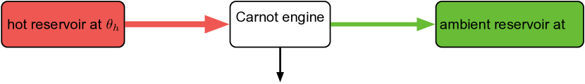
Figure 1: A Carnot engine operating between two isothermal reservoirs. In each cycle, the fictitious engine consumes the heat $Q_{\text{in}}$ at the temperature level $\theta_{h}$ and rejects the heat $Q_{\text{out}}$ at the temperature level $\theta_{0}$ to perform the work $W_{\text{out}}$. Entropy is conserved.

Figure 1 depicts a Carnot engine extracting work from a hot reservoir with constant temperature $\theta_{h}$. The reversible heat intake per cycle $Q_{\text{in}}>0$ is associated with an entropy intake $s_{\text{in}}=Q_{\text{in}}/\theta_{h}>0$. Cyclic operation implies that entropy cannot accumulate in the engine. Reversible operation implies that no entropy is generated in the engine. Consequently, the intake of entropy $s_{\text{in}}$ is balanced by a discharge of entropy $s_{\text{out}}=s_{\text{in}}$. This is associated with a reversible discharge of heat $Q_{\text{out}}=\theta_{0}\,s_{\text{out}}>0$ to the ambient reservoir at constant temperature $\theta_{0}$.

The entropy balance equation $s_{\text{out}}=s_{\text{in}}$ can thus be written as

$$\frac{1}{\theta_{h}}\,Q_{\text{in}}\>=\>\frac{1}{\theta_{0}}\,Q_{\text{out}}\,.$$ (1)

This yields the energy balance equation

$$W_{\text{out}}\>=\>Q_{\text{in}}\>-\>Q_{\text{out}}\>\overset{\eqref{eq:carnot_entropy_balance}}{=}\>Q_{\text{in}}\>-\>\frac{\theta_{0}}{\theta_{h}}\,Q_{\text{in}}\\ \>=\>\frac{\theta_{h}-\theta_{0}}{\theta_{h}}\,Q_{\text{in}}\,.$$ (2)

The ratio

$$\eta_{\text{Carnot}}\>=\>\frac{\theta_{h}-\theta_{0}}{\theta_{h}}\><\>1$$ (3)

is called Carnot efficiency and expresses how much work $W_{\text{out}}$ can be obtained for a given heat intake $Q_{\text{in}}$ in the reversible limit. Consequently, we call $\dot{W}=\eta_{\text{Carnot}}\>\dot{Q}$ the exergetic power of the heat source and note that it is defined relative to a fixed reference temperature $\theta_{0}$. Heat exchanged at a higher temperature carries more exergy.

As an aside, when irreversibility of thermal conduction is considered, the efficiency in the opposite extreme (maximum-work or ‘free-fuel’ limit) was studied via the Curzon-Ahlborn engine [69, 70]. Surprisingly, it turns out to be of a similar form, namely $\eta_{\text{CA}}=1-\sqrt{\theta_{0}/\theta_{h}}$. For exergetic port-Hamiltonian systems, the Carnot efficiency is immediately relevant, since Dirac structures model reversible exchange of power, generalizing ideal wires from circuit theory.

3.2 Exergetic storage function

Let us consider a closed and isochoric system with entropy $s$ and internal energy $u$ given according to its fundamental equation $u=U(s)$. We assume that the system is in equilibrium with itself but not necessarily with its environment. The system’s exergy $A$ is

$$A(s)\>=\>U(s)\>-\>U(s_{0})\>-\>\theta_{0}\left(s-s_{0}\right)$$ (4)

where $s_{0}$ is its entropy once the overall system has reached its equilibrium state. Thus, an infinitesimal change of exergy is written as $\differential A=\bigl{(}\theta(s)-\theta_{0}\bigr{)}\,\differential s$ with $\theta(s)=\partialderivative{U(s)}{s}$. Reversible exchange of heat power $\dot{Q}$ at the temperature level $\theta$ is associated with an entropy exchange rate $\dot{s}=\frac{1}{\theta}\,\dot{Q}$. Consequently, the corresponding exergetic power is given as

$$\dot{A}=\bigl{(}\theta(s)-\theta_{0}\bigr{)}\dot{s}=\frac{\theta-\theta_{0}}{\theta}\,\dot{Q}\,.$$ (5)

The exergetic power $\dot{A}$ is equal to the (energetic) thermal power $\dot{Q}$ multiplied with the Carnot efficiency which is defined by the temperature $\theta$ at which the thermal power is exchanged and the environment temperature $\theta_{0}$, see Equation 3.

Now, let us consider a closed system with entropy $s$, volume $v$, and internal energy $u$ given according to its fundamental equation $u=U(s,v)$. The system further has potential energy $E_{\text{pot}}$ depending on its configuration $q$ and kinetic energy $E_{\text{kin}}$ depending on its momentum $p$. Its exergy $A$ is

$$A(s,v,q,p)\>=\>U(s,v)-U(s_{0},v_{0})\>-\>\theta_{0}\left(s-s_{0}\right)\>+\>\pi_{0}\left(v-v_{0}\right)\>+\\ +\>E_{\text{pot}}(q)-E_{\text{pot}}(q_{0})\>+\>E_{\text{kin}}(p)\,.$$ (6)

The exergy function is obtained from the energy function by adding linear terms which determine the equilibrium and constant terms which make the exergy zero at equilibrium. The physical meaning of the term linear in $s$ has been explained above using the Carnot engine as a theoretical device. The meaning of the term linear in $v$ can be explained as follows: The infinitesimal change of exergy caused by an infinitesimal change of volume is $\bigl{(}\pi(s,v)-\pi_{0}\bigr{)}\,\differential v$ with pressure $\pi(s,v)=-\partialderivative{U(s,v)}{v}$. If the system expands at the rate $\dot{v}$, it has to displace the atmosphere which is assumed to have a fixed pressure $\pi_{0}$. This requires the mechanical power $\pi_{0}\,\dot{v}$. Hence, only $\left(\pi-\pi_{0}\right)\dot{v}$ remains as exergetic power. The first line in Equation 6 represents the physical exergy, while the second line represents the (macroscopic) mechanical energy/exergy. The constant $-E_{\text{pot}}(q_{0})$, corresponding to the configuration with least potential energy, makes the total exergy zero in the equilibrium state.

In the sequel, we usually omit the constant terms in the exergy function to save space and because in practice these constants are often not known a priori. In general, we consider potentials differing only by an additive constant to be equivalent.

3.3 Two similar viewpoints

According to 2.10, the state of a GENERIC system evolves according to $\dot{x}^{i}=L^{ij}(x)\,\partialderivative{E}{x^{j}}+M^{ij}(x)\,\partialderivative{S}{x^{j}}$. Using the degeneracy conditions, we can rewrite this as

$$\dot{x}^{i}\>=\>\left(\theta_{0}\,L^{ij}(x)-M^{ij}(x)\right)\partialderivative{\Phi}{x^{j}}$$ (7a)

with a single generating function $$\Phi=-S+\frac{1}{\theta_{0}}\,E+\frac{\pi_{0}}{\theta_{0}}\,V-\frac{\mu_{0}}{\theta_{0}}\,N \frac{1}{\theta_{0}},\,\frac{\pi_{0}}{\theta_{0}},\,\frac{\mu_{0}}{\theta_{0}}\in\mathbb{R}^{+} x_{0} \Phi x_{0} \Phi$$ where are some constant multipliers. The GENERIC models the approach to the equilibrium state and is a Lyapunov function for the stability of  [33, 36]. Adding some constant shifts, can equivalently be defined as

$$\Phi(x)=-S(x)+\frac{1}{\theta_{0}}\bigl{(}E(x)-E(x_{0})\bigr{)}+\frac{\pi_{0}}{\theta_{0}}\bigl{(}V(x)-V(x_{0})\bigr{)}-\frac{\mu_{0}}{\theta_{0}}\bigl{(}N(x)-N(x_{0})\bigr{)}\,.$$ (7b)

Equation 7b shows the relationship between GENERIC and the maximum entropy principle: The equilibrium state $x_{0}$ maximizes the entropy $S$ under the constraints of constant total energy $E$, volume $V$, and mass $N$. Thus, $\frac{1}{\theta_{0}}$, $\frac{\pi_{0}}{\theta_{0}}$ and $\frac{\mu_{0}}{\theta_{0}}$ can be seen as Lagrange multipliers for constraints stemming from fundamental conservation laws that hold for isolated systems. The multipliers are thus determined by the values of the intensive variables at equilibrium, as already suggested by the notation.

We can also write the GENERIC in the unconventional, yet equivalent form

$$\dot{x}^{i}\>=\>\left(L^{ij}(x)-\frac{1}{\theta_{0}}M^{ij}(x)\right)\partialderivative{A}{x^{j}}$$ (8a)

with generating function

$$A(x)\>=\>E(x)-E(x_{0})-\theta_{0}\bigl{(}S(x)-S(x_{0})\bigr{)}+\pi_{0}\bigl{(}V(x)-V(x_{0})\bigr{)}-\mu_{0}\bigl{(}N(x)-N(x_{0})\bigr{)}\,.$$ (8b)

While Equation 7b corresponds to maximizing entropy subject to constraints which must be satisfied for an isolated system, Equation 8b corresponds to minimizing the exergy function defined by Equation 8b. If we consider a system consisting of a subsystem (body) together with an infinitely large environment (medium), Equation 8b may be seen as a Lagrangian for the maximum amount of work $E(x)-E(x_{0})$ that can be extracted from the overall system while keeping its total entropy $S$, the volume $V$ and the mass $N$ constant. Since the medium is infinitely large, its intensive variables are equal to the intensive variables of the overall system at equilibrium. These variables are the Lagrange multipliers $\theta_{0},\,\pi_{0},\,\mu_{0}$. Of course, Equation 8b is also a Lyapunov function for thermodynamic equilibrium. This makes immediate sense since, again, exergy is the amount of work which can be extracted from the system until it reaches thermodynamic equilibrium where no (spontaneous) changes can occur [6].

We conclude that we are dealing with two similar viewpoints, namely one which is biased towards entropy and relaxation and another one which is biased towards energy and its degradation. The former is more natural for the GENERIC framework, while the latter is taken by exergetic port-Hamiltonian systems.

4 Isothermal systems

In this section, we introduce classical dissipative port-Hamiltonian systems by means of the simplest example, namely the damped harmonic oscillator. After a discussion of the physical meaning of the Hamiltonian function, we will see how a subtle modification of the oscillator model leads us to an isothermal exergetic port-Hamiltonian system. We conclude that the present framework is a straightforward extension of the classical theory. The extension provides a thermodynamic structure to port-Hamiltonian systems which can be understood as a compositional version of the GENERIC structure.

4.1 Classical port-Hamiltonian systems

In the classical port-Hamiltonian framework, physical systems are ultimately comprised of energy storage components, energy routing components, and (free) energy dissipating components, as the following example shows:

Example 4.1 (classical model of the damped harmonic oscillator).

The free vibration of the damped oscillator in Figure 2(a) is commonly modelled via the differential equation $m\,\ddot{q}+d\,\dot{q}+\frac{1}{c}\,q\,=\,0$, where $q$ is the displacement, $m$ is the mass, $d$ is the damping coefficient, and $c$ is the spring compliance.

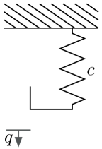
(a) sketch

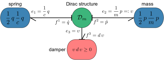
(b) bond-graph expression

Figure 2: Damped harmonic oscillator.

The port-Hamiltonian formulation uses separate state variables for each storage component, namely the extension of the spring $q$ and the momentum of the mass $p$. Figure 2(b) shows a bond-graph expression of the port-Hamiltonian system. Regarding the syntax, blue boxes represent storage components, green boxes represent the Dirac structure, and red boxes represent the resistive structure. The sum of the terms annotated inside the blue boxes represents the Hamiltonian $H$. The term annotated inside the red box represents the dissipated power. An arrowhead on every bond indicates the direction in which power flows when the respective pairing $e_{i}\,f^{i}$ (fixed $i$) takes a positive value. We fix this direction such that positive values correspond to stored power, dissipated power, and power supplied to other systems. This will allow us to eventually omit the arrowheads resulting in clearer diagrams and simplified communication. For now, we also annotate each bond with a causal stroke: A transversely-oriented bar is placed on that end which assigns the value of the flow variable, see 4.3 at the end of the section. In this article, we additionally annotate each bond with formulaic expressions of its associated flow and effort variables.

The state $x=\left(q,\,p\right)\in\mathcal{X}=\mathbb{R}^{2}$ evolves according to

$$\left(f^{1},\,f^{2},\,e_{1},\,e_{2}\right)\> =\>\left(\dot{q},\,\dot{p},\,\frac{\partial H}{\partial q}(x),\,\frac{\partial H}{\partial p}(x)\right)$$ (9a)

$$\left[\begin{array}[]{c}f^{1}\\ f^{2}\\ \hline\cr e_{3}\end{array}\right]\> =\>\left[\begin{array}[]{rr|r}0&1&0\\ -1&0&-1\\ \hline\cr 0&1&0\end{array}\right]\,\left[\begin{array}[]{c}e_{1}\\ e_{2}\\ \hline\cr f^{3}\end{array}\right]$$ (9k)

$$f^{3}\> =\>d\,e_{3}\,.$$ (9l)

Equation 9a defines the storage port (blue components). The matrix in Equation 9k defines the Dirac structure (green component), see 2.11. Its first two rows (and columns) are related to storage and thus to the bundle $T\mathcal{X}\oplus T^{*}\mathcal{X}$. The last row is related to the trivial bundle $\mathbb{R}\times\mathbb{R}^{*}\rightarrow\mathcal{X}$ which also appears in the definition of the resistive structure (red component) based on Equation 9l, see 2.12. Damper and mass interact via the power-conjugate variables $e_{3}=\upsilon$ (velocity) and $f^{3}=d\,\upsilon$ (damping force). The Hamiltonian $H\colon\mathcal{X}\rightarrow\mathbb{R}$ is the same as in 2.4. Since $H$ is bounded from below, the system is passive. ∎

The damper represents an irreversible process that conserves energy as it turns work into heat. However, Figure 2(b) shows the damper as a one-port component and the power $e_{3}\,f^{3}$ going into it disappears, meaning that it is not balanced by an outgoing power of equal amount. Thus, there is an obvious discrepancy between the port-Hamiltonian structure and the first law of thermodynamics, at least as long as we believe that the Hamiltonian represents energy in the thermodynamic sense.

For classical port-Hamiltonian systems we can argue from a thermodynamics viewpoint as follows: A reversible interaction with a thermal reservoir of constant temperature is (implicitly) assumed in the modelling process. The interaction maintains thermal equilibrium of the system and the (waste heat) reservoir (i.e. environment), thereby making the overall system isothermal.

In [23] (p. 25), it is stated that the physical meaning of the Hamiltonian (of a classical dissipative port-Hamiltonian system) is ‘free energy’, rather than energy. In equilibrium thermodynamics, the Helmholtz free energy is a thermodynamic potential obtained from the internal energy via a Legendre transformation with respect to entropy. A potential contains all thermodynamic information about the behaviour of a material at equilibrium, see e.g. [36] (p. 10). The thermodynamic potential named after Helmholtz is called a free energy because the maximum entropy principle applied to an isothermal and isochoric non-equilibrium system implies the minimization of its free energy. The difference between its free energy in the initial state and its free energy in the equilibrium state corresponds to the maximum (reversible) work production which can occur as the system passes from the initial to the equilibrium state while interacting with the isothermal reservoir at the same temperature, see e.g. [68] (ch. 6). The statement that the Hamiltonian is a ‘free energy’ can thus be explained as follows: An (irrelevant) additive constant in the Hamiltonian may be identified with the combined Helmholtz free energy corresponding to all (neglected) internal energy storage of the overall system. Hence, the term ‘free energy’, as used in [23], additively combines electro-mechanical energy components and (constant) Helmholtz free energy components corresponding to internal energy storage in the isothermal system and environment. The electro-mechanical energy components have no entropy content since all related degrees of freedom are resolved by the model. Therefore, they are not Legendre-transformed quantities. In this (perhaps not obvious) sense, the Hamiltonian is a (Helmholtz) free energy. The GENERIC literature also mentions that Helmholtz free energy can be used as a single generator for isothermal systems [36] (p. 136).

The idea of summing different electro-mechanical and ‘free energy’ components is more commonly understood within the more general exergy concept. Indeed, for isothermal and isochoric systems, the total Helmholtz free energy essentially coincides with exergy. Similarly, for isothermal and isobaric systems, the total Gibbs free energy essentially coincides with exergy, see [6].

Inspired by bond-graph modelling, the wish to model non-isothermal systems and to fully express the first law within the port-Hamiltonian framework first led to the use of lossless systems, see e.g. [23]. For Equation 9, this means that a thermal port is added to the damper, making it a power-conserving component. Obviously, the passivity property of being lossless relates only to the first law of thermodynamics and ignores the second law of thermodynamics and all its implications.

4.2 Isothermal exergetic port-Hamiltonian systems

In contrast, exergetic port-Hamiltonian systems are coherent with both the first and the second law of thermodynamics and link passivity to degradation of energy. We consider the oscillator from Equation 9 as an exergetic port-Hamiltonian system:

Example 4.2 (exergetic model of the damped harmonic oscillator).

Let us explicitly assume that the system is isothermal because it is in thermal equilibrium with its environment having constant temperature $\theta_{0}$. We consider the environment as an (infinitely large) thermal reservoir. We need not consider for instance its volume, mass or chemical composition because at this point only thermal interaction with the environment is relevant. From the isothermal condition

$$\theta_{0}\overset{!}{=}\theta(s)=\partialderivative{U(s)}{s}\,,$$

it follows that $u=U(s)=\theta_{0}\,s$ is a fundamental equation for the environment. Its exergy content with respect to itself is $U(s)-\theta_{0}\,s=0$, see Equation 4. Thus, the Hamiltonian already is (or at least can be interpreted as) an exergetic storage function.

Since the damper remains at $\theta_{0}$, its exergetic heating power is zero. Therefore, it might seem reasonable to omit its thermal port, cf. [23] (p. 25). However, for exergetic port-Hamiltonian systems, this is made (or kept) explicit, as shown in Figure 3:

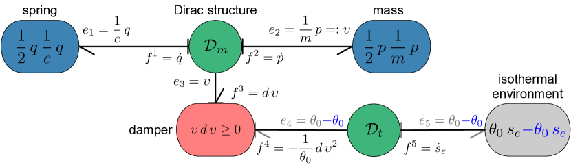
Figure 3: The exergetic port-Hamiltonian model includes the reversible exchange of heat between the damper and the isothermal environment via the Dirac structure $\mathcal{D}_{t}$.

The environment is like a storage component containing zero exergy. According to the assumption, the damper is held at the environment temperature ($e_{4}=\theta_{0}-\theta_{0}=0$). Consequently, the exergetic power $e_{4}\,f^{4}=e_{5}\,f^{5}$ vanishes. The net power at the damper $e_{3}\,f^{3}+e_{4}\,f^{4}=d\,\upsilon^{2}$ is its exergy destruction rate (or dissipated power).

The state $x=\left(q,\,p,\,s_{e}\right)\in\mathcal{X}=\mathbb{R}^{3}$ evolves according to

$$\left(f^{1},\,f^{2},\,f^{5},\,e_{1},\,e_{2},\,e_{5}\right)\> =\>\left(\dot{q},\,\dot{p},\,\dot{s}_{e},\,\frac{\partial H}{\partial q}(x),\,\frac{\partial H}{\partial p}(x),\,0\right)$$ (10a)

$$\left[\begin{array}[]{c}f^{1}\\ f^{2}\\ \hline\cr e_{3}\end{array}\right]\> =\>\left[\begin{array}[]{rr|r}0&1&0\\ -1&0&-1\\ \hline\cr 0&1&0\end{array}\right]\,\left[\begin{array}[]{c}e_{1}\\ e_{2}\\ \hline\cr f^{3}\end{array}\right]$$ (10k)

$$\left[\begin{array}[]{c}f^{5}\\ \hline\cr e_{4}\end{array}\right]\> =\>\left[\begin{array}[]{r|r}0&-1\\ \hline\cr 1&0\end{array}\right]\,\left[\begin{array}[]{c}e_{5}\\ \hline\cr f^{4}\end{array}\right]$$ (10r)

$$\left[\begin{array}[]{c}f^{3}\\ f^{4}\end{array}\right]\> =\>\frac{1}{\theta_{0}}\,d\,\left[\begin{array}[]{rr}\theta_{0}&-\upsilon\\ -\upsilon&\frac{{\upsilon}^{2}}{\theta_{0}}\end{array}\right]\,\left[\begin{array}[]{c}e_{3}\\ e_{4}\end{array}\right]$$ (10y)

where $$\upsilon=\frac{1}{m}\,p$$.

Equation 10a defines the storage port. The mass and the spring are mechanical components containing pure exergy. Therefore, no shift appears in their contribution to the Hamiltonian. The last component of the storage port corresponds to the environment. Equation 10k defines the $\mathcal{D}_{m}$ component ($m$ for mechanical) and Equation 10r defines the $\mathcal{D}_{t}$ component ($t$ for thermal) of the Dirac structure. Finally, Equation 10y defines the resistive structure.

While the diagrammatic expression for the mathematical model structure might seem unnecessarily complicated at first, the $\mathcal{D}_{t}$ component represents that the interaction of the damping process and the environment is a reversible one. At $\mathcal{D}_{t}$, local conservation of entropy holds ($f^{5}=-f^{4}$).

Regarding the syntax, it is not meaningful to directly connect a blue component (exposing a storage port) with a red component (defining resistive structure). The green components (defining reversible interconnection) mediate all exergy exchange.

By removing the shifts written in blue in Figure 3, we obtain a lossless energetic port-Hamiltonian system, asserting that the damper conserves energy, see 4.5. Equivalently, we can assert that $\left(e_{3},\,e_{4}\right)=\left(\upsilon,\,\theta_{0}\right)$ lies in the kernel of the matrix in Equation 10y.

Equation 10 reduces to

$$\dot{q} =\upsilon$$ (11a)

$$\dot{p} =-\frac{1}{c}\,q-d\,\upsilon$$ (11b)

$$\dot{s}_{e} =\frac{1}{\theta_{0}}\,d\,\upsilon^{2}\,.$$ (11c)

However, for the seemingly simpler system in Equation 11, checking thermodynamic consistency is much harder, especially for a computer. For more complex, practical examples, a structured and compositional modelling framework with a diagrammatic syntax is clearly superior. ∎

We arrive at the following conclusion: If we assume that a classical dissipative port-Hamiltonian system is in thermal equilibrium with its isothermal (and isobaric) environment then its Hamiltonian represents the exergy of the overall system. The suggested framework thus is a straigtforwad extension of the classical theory.

Remark 4.3 (causal strokes).

Causal strokes do not indicate physical causality but mark how information propagates when using an explicit time-integration scheme. Hence, at storage components, flows must be inputs. If a consistent computational causality assignment is not possible for all storage components, the model yields an implicit system of differential-algebraic equations (DAE). For instance, placing two capacitors directly in parallel results in an algebraic constraint demanding equality of voltages. In this case, inconsistent initial conditions for the DAE system are related to the ‘two capacitor paradox’. The degeneracy could be avoided by taking into account the resistance of the wire that connects the capacitors. ∎

Remark 4.4 (input-output systems).

The matrix in Equation 9k is of the form

$$\left[\begin{array}[]{c|c}L^{\sharp}&-g\\ \hline\cr{}g^{*}&0\end{array}\right]\,.$$

According to 2.11, it defines a Dirac structure on $T\mathcal{X}\oplus\mathcal{F}_{R}$ where $\mathcal{F}_{R}=\mathcal{X}\times\mathbb{R}$ is the trivial vector bundle on which the resistive structure is defined. We focus on the class of input-output systems where the bottom-right block is zero. The top-left block defines a Poisson structure on $\mathcal{X}$ and thus a Dirac structure $\mathcal{D}_{T\mathcal{X}}$ on $T\mathcal{X}$. The top-right block defines a vector bundle map $-g\colon\mathcal{F}_{R}\rightarrow T\mathcal{X}$ covering the identity on $\mathcal{X}$. The bottom-left block defines its negative dual $g^{*}$. According to Definition 4.2 in [19], $\left(T\mathcal{X},\,\mathcal{F}_{R},\,\mathcal{D}_{T\mathcal{X}},\mathcal{F}_{R}\oplus\mathcal{F}_{R}^{*},\,g\right)$ is an open forward input-output structure. Our impression is that [19] introduces a theoretically very appealing and possibly also practically useful framework for expressing the interconnection of port-Hamiltonian systems. However, Dirac structures which can directly connect a resistive and a boundary port or two different boundary ports (feed-through) are quite important in practice. ∎

Remark 4.5 (classical bond graphs with thermal port).

Let us assume for a moment that the annotated bond-graph expressions shown in this work are merely figures, rather than (yet to be defined) mathematical objects in their own right. Then, we could say that removing all shifts in the annotated components of the storage function and in the annotated expressions for the effort variables manipulates such a figure into a classical energetic bond graph corresponding to a lossless port-Hamiltonian system whose passivity property is tantamount to the first law of thermodynamics only. However, there is no corresponding straightforward modification of the equations defining the resistive structure. This is no surprise since lossless systems have no resistive structure. The red boxes must turn into power-preserving transformers. Of course, the given annotated expressions for the flows at the red boxes can straightforwardly be manipulated into the equations defining these transformers by writing them in terms of the efforts (without shifts) at the red boxes. It is important to note that the resulting equations do not follow from a structured representation enjoying certain properties, as it is the case for resistive structures in the exergetic port-Hamiltonian framework. ∎

5 Non-isothermal systems

We now come to physical modelling of non-isothermal systems. The following example shows that the Carnot efficiency naturally appears in the pairing of effort and flow variables of a bond representing (reversible) exchange of heat.

Example 5.1 (Carnot engine).

Figure 4: Bond-graph expression of a Carnot engine.

Figure 4 shows a bond-graph expression of a Carnot engine operating between a thermal reservoir at temperature $\theta_{h}$ and the environment at temperature $\theta_{0}$ which serves as a reference to define the exergetic storage function $H=H_{h}+H_{e}=H_{h}$. Again, by ignoring the shifts, we obtain the energetic power balance $\dot{Q}_{\text{in}}=\dot{Q}_{\text{out}}+\dot{W}_{\text{out}}$. Due to reversible operation, the exergetic power $-e_{1}\,f^{1}$ going into the engine is fully converted into work $e_{3}\,f^{3}$:

$$e_{3}\,f^{3}=-e_{1}\,f^{1}=-\partialderivative{H_{h}(s_{h})}{s_{h}}\,\dot{s}_{h}=-\left(\theta_{h}-\theta_{0}\right)\left(-\frac{1}{\theta_{h}}\,\dot{Q}_{\text{in}}\right)=\eta_{\text{Carnot}}\,\dot{Q}_{\text{in}}$$

According to the first law of thermodynamics, all physical systems are cyclo-lossless if the storage function represents energy. In contrast, only perfectly reversible devices, like the Carnot engine, are cyclo-lossless if the storage function represents exergy. ∎

For defining the exergetic storage function of a thermodynamic system, we need to know its internal energy as a function of entropy. In Figure 4 the thermal reservoir has a linear and thus unbounded energy function, reflecting infinite capacity. Alternatively, we could use entropy as a function of internal energy. The next example compares the two choices:

Example 5.2 (gas-filled compartment).

(a) entropy as state variable

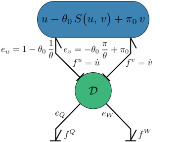
(b) internal energy as state variable

Figure 5: Bond-graph expressions of a compartment with heat and work exchange.

Figure 5 shows two bond-graph expressions for a gas-filled compartment with boundary ports for the exchange of thermal exergetic power $e_{Q}\,f^{Q}$ and work $e_{W}\,f^{W}$. $f^{Q}$ is the rate of entropy leaving the system, $f^{W}$ is its rate of compression, $e_{Q}$ is its temperature, and $e_{W}$ is its negative pressure, both relative to the environment. Figure 5(a) uses entropy and volume as state variables. Since exchange of heat/work does not change volume/entropy, $\mathcal{D}_{t}$ and $\mathcal{D}_{m}$ have the same trivial form as $\mathcal{D}_{t}$ in Figure 3 and Equation 10r. Figure 5(b) uses internal energy and volume as state variables. Exchange of work changes both variables, leading to coupling. Since entropy is used as a potential, $\mathcal{D}$ is modulated according to $\partialderivative{S}{u}=\frac{1}{\theta}$, $\partialderivative{S}{v}=\frac{\pi}{\theta}$. It is defined by

$$\left[\begin{array}[]{c}f^{u}\\ f^{v}\\ \hline\cr e_{Q}\\ e_{W}\end{array}\right]\>=\>\left[\begin{array}[]{cc|cc}0&0&-1/\left(\frac{1}{\theta}\right)&\left(\frac{\pi}{\theta}\right)/\left(\frac{1}{\theta}\right)\\ 0&0&0&-1\\ \hline\cr 1/\left(\frac{1}{\theta}\right)&0&0&0\\ -\left(\frac{\pi}{\theta}\right)/\left(\frac{1}{\theta}\right)&1&0&0\end{array}\right]\,\left[\begin{array}[]{c}e_{u}\\ e_{v}\\ \hline\cr f^{Q}\\ f^{W}\end{array}\right]\,.$$

We will henceforth use internal energy as a (local) thermodynamic potential, since this yields to simpler models. ∎

Next, we consider again the damped harmonic oscillator but this time without assuming thermal equilibrium with the environment.

Example 5.3 (non-isothermal damped harmonic oscillator).

In contrast to Equation 11, we model the damper with a thermal capacity characterized by an energy function $U$, allowing it to heat up. Further, we model heat transfer characterized by a coefficient $\alpha$, allowing the damper to cool down again. Figure 6 shows the model. Equations defining the Dirac structure according to 2.11 and the resistive structure according to 2.12 are annotated.

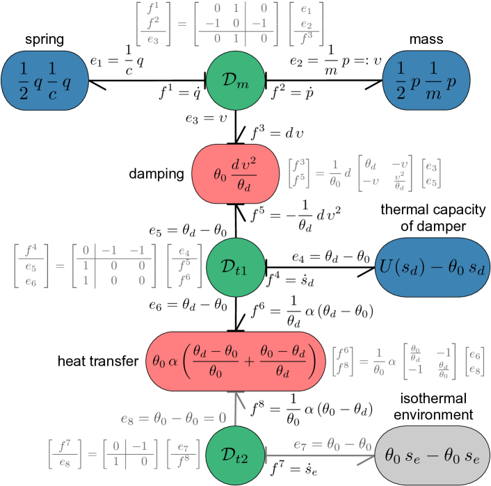
Figure 6: Bond-graph expression of a non-isothermal damped harmonic oscillator.

The damper consumes the mechanical power $e_{3}\,f^{3}$ and produces the thermal exergetic power $-e_{5}\,f^{5}=\frac{\theta_{d}-\theta_{0}}{\theta_{d}}\,d\,\upsilon^{2}$ which is its heat release rate $d\,\upsilon^{2}$ multiplied by the efficiency of a Carnot engine operating between the temperature level of the damper $\theta_{d}=\frac{\partial U(s_{d})}{\partial s}$ and that of the environment $\theta_{0}$. The net exergetic power at the damper $e_{3}\,f^{3}+e_{5}\,f^{5}=\theta_{0}\,\frac{d\,\upsilon^{2}}{\theta_{d}}$ is its exergy destruction rate which is its entropy production rate $\frac{d\,\upsilon^{2}}{\theta_{d}}$ multiplied by the environment temperature.

Once $\theta_{d}>\theta_{0}$, heat is irreversibly transferred from the damper’s thermal capacity to the environment, destroying exergy at the rate $e_{6}\,f^{6}+e_{8}\,f^{8}$. We have $e_{8}\,f^{8}=0$ because heat at the environment temperature cannot be used to do work. ∎

In summary, the green components define the Dirac structure which encodes reversible (lossless) exchange of exergy. The net exergetic power at every green component is zero. Energy and entropy are conserved. The red components define the resistive structure which encodes irreversible processes (relaxation). At every red component, the net energetic power is zero. At the same time, entropy is produced (or conserved), implying a loss (or conservation) of exergy. Cyclo-passivity consequently corresponds to the fact that exergy is either conserved or destroyed.

We now model an isolated cylinder-piston device both as an exergetic port-Hamiltonian system and as a GENERIC system.

Example 5.4 (isolated cylinder-piston device).

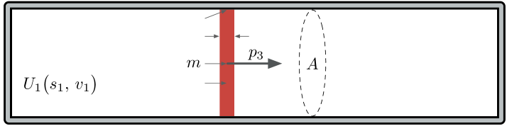
Figure 7: Isolated cylinder of cross-sectional area $A$ containing a piston with mass $m$ and momentum $p_{3}$. The gas in both compartments exchanges heat (coefficient $\alpha$) with the piston. When the piston moves, heat is added to it due to friction (coefficient $d$).

Figure 8: Bond-graph expression of the isolated cylinder-piston device in Figure 7.

Figure 7 shows a system comprising of two compartments filled with a fixed amount of ideal gas which are separated by a piston. Its state is

$$x=\left(s_{1},\,v_{1},\,s_{2},\,v_{2},\,s_{3},\,p_{3}\right)\in\mathcal{X}\subset\mathbb{R}^{6}\,.$$

Given that $U_{1}$, $U_{2}$, and $U_{3}$ are expressions for the internal energy of the two compartments and the piston, we define functions $E,\,S,\,V,\,H\in C^{\infty}(\mathcal{X})$ for total energy, entropy, volume and exergy by

$$E(x) =U_{1}(s_{1},\,v_{1})+U_{2}(s_{2},\,v_{2})+U_{3}(s_{3})+{(p_{3})}^{2}/(2\,m)$$ (12a)

$$S(x) =s_{1}+s_{2}+s_{3}$$ (12b)

$$V(x) =v_{1}+v_{2}$$ (12c)

$$H(x) =E(x)-\theta_{0}\,S(x)+\pi_{0}\,V(x)+\mathrm{const.}$$ (12d)

where $\theta_{0},\,\pi_{0}\in\mathbb{R}^{+}$ are the (now arbitrary) reference temperature and pressure, see Equation 6.

The Dirac structure $\mathcal{D}_{m}$ is defined by

$$\left[\begin{array}[]{c}f^{1}\\ f^{2}\\ f^{3}\\ \hline\cr e_{4}\end{array}\right]=\left[\begin{array}[]{rrr|r}0&0&A&0\\ 0&0&-A&0\\ -A&A&0&-1\\ \hline\cr 0&0&1&0\end{array}\right]\,\left[\begin{array}[]{c}e_{1}\\ e_{2}\\ e_{3}\\ \hline\cr f^{4}\end{array}\right].$$

The degeneracy of the top-left block corresponds to the (symplectic) Casimir $v_{1}+v_{2}$. The Dirac structures $\mathcal{D}_{t1}$, $\mathcal{D}_{t2}$ and $\mathcal{D}_{t3}$ are defined basically as in Figure 6.

The resistive structure corresponding to the damping is defined by

$$\begin{bmatrix}f^{4}\\ f^{12}\end{bmatrix}=\underbrace{\frac{1}{\theta_{0}}\,d\,\begin{bmatrix}\theta_{3}&-\upsilon_{3}\\ -\upsilon_{3}&\frac{{(\upsilon_{3})}^{2}}{\theta_{3}}\end{bmatrix}}_{R(x)}\,\begin{bmatrix}e_{4}\\ e_{12}\end{bmatrix}=\underbrace{\begin{bmatrix}\frac{1}{\upsilon_{3}}\\ -\frac{1}{\theta_{3}}\end{bmatrix}}_{C(x)}\underbrace{\begin{bmatrix}\frac{1}{\theta_{0}}\,d\,{(\upsilon_{3})}^{2}\,\theta_{3}\end{bmatrix}}_{D(x)}\underbrace{\begin{bmatrix}\frac{1}{\upsilon_{3}}&-\frac{1}{\theta_{3}}\end{bmatrix}}_{C^{\mathrm{T}}(x)}\,\underbrace{\begin{bmatrix}\upsilon_{3}\\ \theta_{3}-\theta_{0}\end{bmatrix}}_{e}.$$

The factorization $R(x)=C(x)\,D(x)\,C^{\mathrm{T}}(x)$ shows positive semidefiniteness. Energy is conserved since $C^{\mathrm{T}}(x)\,\begin{bmatrix}\upsilon_{3}&\theta_{3}\end{bmatrix}^{\mathrm{T}}=0$. The remaining term $-\theta_{0}$ in $e_{12}$ comes from $-\theta_{0}\,S(x)$ in $H$, reflecting that the entropy function generates the gradient dynamics. The resistive structure corresponding to thermal conduction between the left compartment and the piston is defined by

$$\begin{bmatrix}f^{6}\\ f^{10}\end{bmatrix}=\frac{1}{\theta_{0}}\,\alpha\,\begin{bmatrix}\frac{\theta_{3}}{\theta_{1}}&-1\\ -1&\frac{\theta_{1}}{\theta_{3}}\end{bmatrix}\,\begin{bmatrix}e_{6}\\ e_{10}\end{bmatrix}=\begin{bmatrix}\frac{1}{\theta_{1}}\\ -\frac{1}{\theta_{3}}\end{bmatrix}\begin{bmatrix}\frac{1}{\theta_{0}}\,\alpha\,{\left(\sqrt{\theta_{1}\,\theta_{3}}\right)}^{2}\end{bmatrix}\begin{bmatrix}\frac{1}{\theta_{1}}&-\frac{1}{\theta_{3}}\end{bmatrix}\,\begin{bmatrix}\theta_{1}-\theta_{0}\\ \theta_{3}-\theta_{0}\end{bmatrix}.$$

The factorization has a physical interpretation in terms of LIT: $C^{\mathrm{T}}(x)\,e$ is the thermodynamic force, $D(x)$ is the linear relation containing the relaxation/transport coefficients, and thus $D(x)\,C^{\mathrm{T}}(x)\,e$ is the thermodynamic flux, see [35]. We compare this (without much rigor) to a weak-formulation of distributed-parameter thermal conduction [46] which we reformulate in the language of exterior calculus:

$$\langle\varphi,R(x)\,\psi\rangle=\int_{\mathcal{Z}}\differential\left(\dfrac{1}{\theta}\,\varphi\right)\wedge\star\left(\frac{1}{\theta_{0}}\,\kappa\,\theta^{2}\,\differential\left(\dfrac{1}{\theta}\,\psi\right)\right)$$

Here, $\varphi$ and $\psi$ are test functions. The latter is essentially a place holder for the effort ($0$-form) $e=\theta-\theta_{0}$. The parameter $\kappa$ is the thermal conductivity. For a simple spatial domain $\mathcal{Z}$, where $A$ is a cross section perpendicular to the direction of thermal conduction and $l$ is a length in that direction, the Hodge star $\star$ essentially becomes $\frac{A}{l}$ and $\frac{A}{l}\,\kappa$ indeed corresponds to $\alpha$. In the lumped-parameter setting, the term $\theta^{2}$ is replaced by the squared geometric mean $\theta_{1}\,\theta_{3}$ of the two known temperatures.

The combined Dirac structure $\mathcal{D}\cong\mathcal{D}_{m}\oplus\mathcal{D}_{t1}\oplus\mathcal{D}_{t2}\oplus\mathcal{D}_{t3}$ is defined by

$$\left[\begin{array}[]{c}f^{1}\\ f^{2}\\ f^{3}\\ f^{5}\\ f^{7}\\ f^{9}\\ \hline\cr e_{4}\\ e_{12}\\ e_{6}\\ e_{10}\\ e_{8}\\ e_{11}\end{array}\right]=\left[\begin{array}[]{rrrrrr|rrrrrr}&&A&&&&&&&&&\\ &&-A&&&&&&&&&\\ -A&A&&&&&-1&&&&&\\ &&&&&&&&-1&&&\\ &&&&&&&&&&-1&\\ &&&&&&&-1&&-1&&-1\\ \hline\cr&&1&&&&&&&&&\\ &&&&&1&&&&&&\\ &&&1&&&&&&&&\\ &&&&&1&&&&&&\\ &&&&1&&&&&&&\\ &&&&&1&&&&&&\\ \end{array}\right]\>\left[\begin{array}[]{c}e_{1}\\ e_{2}\\ e_{3}\\ e_{5}\\ e_{7}\\ e_{9}\\ \hline\cr f^{4}\\ f^{12}\\ f^{6}\\ f^{10}\\ f^{8}\\ f^{11}\end{array}\right].$$

The top-left block $L$ defines a Poisson structure $\poissonbracket{\cdot}{\cdot}$ on $\mathcal{X}$. The top-right block $-g$ defines a vector bundle map $g\colon\mathcal{F}_{R}\rightarrow T\mathcal{X}$, see 4.4. The block-diagonal combination of the three tensors defining the component resistive structures defines the combined resistive structure $\mathcal{R}$ on $\mathcal{F}_{R}$. Then $\left(\mathcal{X},\,\mathcal{F}_{R},\,\{0\},\mathcal{D},\,\mathcal{R},\,H\right)$ is a port-Hamiltonian system. Its state evolves according to $\dot{x}=\left(L-g\,R(x)\,g^{*}\right)\differential H$. Let $M=\theta_{0}\,g\,R\,g^{*}$ define a gradient structure $\Psi$ on $\mathcal{X}$. Then $\left(\mathcal{X},\,\poissonbracket{\cdot}{\cdot},\,\Psi,\,E,\,S\right)$ defines a GENERIC system. Its state evolves according to $\dot{x}=L\,\differential E+M(x)\,\differential S$. ∎

The above shows that an isolated exergetic port-Hamiltonian system is equivalent to a GENERIC system and thus it is thermodynamically consistent. It is important to note that the systems in Equation 11 or Figure 6 are also isolated systems (including their environment). In the future, a rigorous compositional framework will enable us to assert thermodynamic consistency for open systems and their interconnection.

In the final example, we consider an electrically-heated cylinder-piston device which exchanges heat and work with the (isothermal and isobaric) environment.

Example 5.5 (heated cylinder-piston device).

Figure 9: An open cylinder with cross-sectional area $A$ and isolating walls contains an electric heater with resistance $R_{h}$. A piston with mass $m$ and momentum $p_{p}$ closes the cylinder. Attached to it is a spring with compliance $c$ and extension $q_{s}$. The gas in the compartment and the environment both exchange heat (coefficient $\alpha$) with the piston. When the piston moves, heat is added to it due to friction (coefficient $d$).

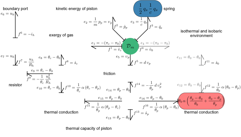
Figure 10: Bond-graph expression of the open cylinder-piston device in Figure 9.

Figure 9 depicts the device, while the bond-graph expression in Figure 10 conveys the structure of the corresponding physical model. The system is open. To determine a dynamics, we have to interconnect the electric boundary port $\left(f^{6},\,e_{6}\right)$ with another system (having the same environment) such that the composite forms an isolated system. We merely state some details which differ from previous examples.

The Dirac structure $\mathcal{D}_{m}$ is defined by

$$\left[\begin{array}[]{c}f^{1}\\ f^{2}\\ f^{3}\\ f^{4}\\ \hline\cr e_{5}\end{array}\right]=\left[\begin{array}[]{rrrr|r}0&A&0&0&0\\ -A&0&-1&A&-1\\ 0&1&0&0&0\\ 0&-A&0&0&0\\ \hline\cr 0&1&0&0&0\end{array}\right]\,\left[\begin{array}[]{c}e_{1}\\ e_{2}\\ e_{3}\\ e_{4}\\ \hline\cr f^{5}\end{array}\right].$$

The degeneracy of the top-left block corresponds to (symplectic) Casimirs $v_{c}+v_{0}$ and $v_{c}/A-q_{s}$. When the gas expands, it has to displace the isobaric environment. The corresponding mechanical work cannot be extracted and hence $e_{4}\,f^{4}=0$. Only the exergetic power $e_{1}\,f^{1}$ could possibly be extracted.

The resistive structure corresponding to the resistor is defined by

$$\begin{bmatrix}f^{7}\\ f^{9}\end{bmatrix}=\frac{1}{\theta_{0}}\,\frac{1}{R_{h}}\,\begin{bmatrix}\theta_{c}&-u_{h}\\ -u_{h}&\frac{{(u_{h})}^{2}}{\theta_{c}}\end{bmatrix}\,\begin{bmatrix}e_{7}\\ e_{9}\end{bmatrix}=\begin{bmatrix}\frac{1}{u_{h}}\\ -\frac{1}{\theta_{c}}\end{bmatrix}\begin{bmatrix}\frac{1}{\theta_{0}}\,\frac{1}{R_{h}}\,{(u_{h})}^{2}\,\theta_{c}\end{bmatrix}\begin{bmatrix}\frac{1}{u_{h}}&-\frac{1}{\theta_{c}}\end{bmatrix}\,\begin{bmatrix}u_{h}\\ \theta_{c}-\theta_{0}\end{bmatrix}$$

which is analogous to the case of friction. ∎

6 Conclusions

The compositional nature of port-Hamiltonian systems makes them attractive for modelling of interconnected and controlled physical systems. The present framework enhances classical port-Hamiltonian theory with a physically sound interpretation of dissipativity and a refined structure that ensures thermodynamic consistency. Future work must address the question how the interconnection of exergetic port-Hamiltonian systems can be formalized and implemented such that thermodynamic consistency of constituent systems implies the consistency of composite systems.

At the heart of this work lies the goal to develop a practical framework to support the design and operation of sustainable energy systems. Not only as a consequence of increasing demand for sustainable technology, teams are becoming more interdisciplinary. This is one important reason why intuitive abstractions with computational meaning are of central importance for the future of engineering. Exergetic port-Hamiltonian systems admit a diagrammatic syntax that is derived form bond-graph modelling. Future work must thus address the question how expressions in this syntax can be formalized as mathematical objects based on which computations can be performed. Once this foundation is established, exergetic port-Hamiltonian systems can become a valuable tool for thermodynamic design and optimization. Their diagrammatic syntax will help humans to think and communicate, while their underlying mathematical framework, together with modern compiler technology, will efficiently handle the tedious parts of computational procedures such as modular and hierarchical composition, model transformations, simulation, optimization, and control design. Since many and eventually possibly all such procedures will provably preserve the compositional and the thermodynamic structure, a lot of effort previously spent on arranging parts, bookkeeping and verification can then be spent on sustainable design.

Disclosure statement

No potential conflict of interest was reported by the authors.

References

- [1] J. Szargut, Exergy Method: Technical and Ecological Applications, WIT Press, 2005.
- [2] Z. Rant, Exergie, ein neues Wort für “technische Arbeitsfähigkeit”, Forschung auf dem Gebiet des Ingenieurwesens A 22 (1) (1956) 33–37. doi:10.1007/BF02592661.
- [3] J. W. Gibbs, A method of geometrical representation of the thermodynamic properties of substances by means of surfaces, Transactions of the Connecticut Academy of Arts and Sciences 2 (1873) 382–404.
- [4] R. A. Gaggioli, D. H. Richardson, A. J. Bowman, Available energy—Part I: Gibbs revisited, Journal of Energy Resources Technology 124 (2) (2002) 105–109. doi:10.1115/1.1448336.
- [5] R. A. Gaggioli, D. M. Paulus, Available energy—Part II: Gibbs extended, Journal of Energy Resources Technology 124 (2) (2002) 110–115. doi:10.1115/1.1448337.
- [6] J. H. Keenan, Availability and irreversibility in thermodynamics, British Journal of Applied Physics 2 (7) (1951) 183–192. doi:10.1088/0508-3443/2/7/302.
- [7] R. A. Gaggioli (Ed.), Thermodynamics: Second Law Analysis, Vol. 122, American Chemical Society, 1980. doi:10.1021/bk-1980-0122.
- [8] T. Kotas, The Exergy Method of Thermal Plant Analysis, Elsevier, 1985. doi:10.1016/c2013-0-00894-8.
- [9] A. Bejan, Entropy generation minimization: The new thermodynamics of finite-size devices and finite-time processes, Journal of Applied Physics 79 (3) (1996) 1191–1218. doi:10.1063/1.362674.
- [10] B. Andresen, Current trends in finite-time thermodynamics, Angewandte Chemie International Edition 50 (12) (2011) 2690–2704. doi:10.1002/anie.201001411.
- [11] M. H. Rubin, Optimal configuration of a class of irreversible heat engines. I, Physical Review A 19 (3) (1979) 1272–1276. doi:10.1103/physreva.19.1272.
- [12] M. H. Rubin, Optimal configuration of a class of irreversible heat engines. II, Physical Review A 19 (3) (1979) 1277–1289. doi:10.1103/physreva.19.1277.
- [13] P. Salamon, J. Nulton, G. Siragusa, T. Andersen, A. Limon, Principles of control thermodynamics, Energy 26 (3) (2001) 307 – 319. doi:10.1016/S0360-5442(00)00059-1.
- [14] J. A. McGovern, F. O’Toole, A virtual-system concept for exergy analysis of flow network plant; part I: Principles, in: Proceedings of International Symposium on Efficiency, Costs, Optimization and Simulation of Energy Systems, New York, NY, 1992, pp. 155–160.
- [15] T. J. Courant, Dirac manifolds, Transactions of the American Mathematical Society 319 (2) (1990) 631–661. doi:10.1090/S0002-9947-1990-0998124-1.
- [16] I. Dorfman, Dirac Structures and Integrability of Nonlinear Evolution Equations, John Wiley, Chichester, 1993.
- [17] M. Dalsmo, A. van der Schaft, On representations and integrability of mathematical structures in energy-conserving physical systems, SIAM Journal on Control and Optimization 37 (1) (1998) 54–91. doi:10.1137/s0363012996312039.
- [18] J. Merker, On the geometric structure of Hamiltonian systems with ports, Journal of Nonlinear Science 19 (6) (2009) 717–738. doi:10.1007/s00332-009-9052-3.
- [19] M. Barbero-Liñán, H. Cendra, E. G.-T. Andrés, D. M. de Diego, New insights in the geometry and interconnection of port-Hamiltonian systems, Journal of Physics A: Mathematical and Theoretical 51 (37) (2018) 375201. doi:10.1088/1751-8121/aad4ba.
- [20] J. C. Willems, Dissipative dynamical systems part I: General theory, Archive for Rational Mechanics and Analysis 45 (5) (1972) 321–351. doi:10.1007/bf00276493.
- [21] A. van der Schaft, L2-Gain and Passivity Techniques in Nonlinear Control, 3rd Edition, Springer International Publishing, 2017. doi:10.1007/978-3-319-49992-5.
- [22] A. van der Schaft, Cyclo-dissipativity revisited, IEEE Transactions on Automatic Control (2020). doi:10.1109/TAC.2020.3013941.
- [23] V. Duindam, A. Macchelli, S. Stramigioli, H. Bruyninckx (Eds.), Modeling and Control of Complex Physical Systems, Springer Berlin Heidelberg, 2009. doi:10.1007/978-3-642-03196-0.
- [24] D. Eberard, B. Maschke, Port Hamiltonian systems extended to irreversible systems: The example of the heat conduction, IFAC Proceedings Volumes 37 (13) (2004) 243–248. doi:10.1016/S1474-6670(17)31230-2.
- [25] H. Ramirez, B. Maschke, D. Sbarbaro, Irreversible port-Hamiltonian systems: a general formulation of irreversible processes with application to the CSTR, Chemical Engineering Science 89 (2013) 223–234. doi:10.1016/j.ces.2012.12.002.
- [26] R. Hermann, Geometry, physics, and systems, M. Dekker, New York, 1973.
- [27] D. Eberard, B. Maschke, A. van der Schaft, An extension of Hamiltonian systems to the thermodynamic phase space: Towards a geometry of nonreversible processes, Reports on Mathematical Physics 60 (2) (2007) 175–198. doi:10.1016/s0034-4877(07)00024-9.
- [28] A. van der Schaft, B. Maschke, Geometry of thermodynamic processes, Entropy 20 (12) (2018) 925. doi:10.3390/e20120925.
- [29] I. Dzyaloshinskii, G. Volovick, Poisson brackets in condensed matter physics, Annals of Physics 125 (1) (1980) 67–97. doi:10.1016/0003-4916(80)90119-0.
- [30] M. Grmela, Particle and bracket formulations of kinetic equations, in: Fluids and plasmas: geometry and dynamics (Boulder, Colo., 1983), Vol. 28 of Contemp. Math., Amer. Math. Soc., Providence, RI, 1984, pp. 125–132. doi:10.1090/conm/028/751978.
- [31] A. N. Kaufman, Dissipative Hamiltonian systems: A unifying principle, Physics Letters A 100 (8) (1984) 419–422. doi:10.1016/0375-9601(84)90634-0.
- [32] P. J. Morrison, Bracket formulation for irreversible classical fields, Physics Letters A 100 (8) (1984) 423–427. doi:10.1016/0375-9601(84)90635-2.
- [33] M. Grmela, H. C. Öttinger, Dynamics and thermodynamics of complex fluids. I. development of a general formalism, Phys. Rev. E 56 (1997) 6620–6632. doi:10.1103/PhysRevE.56.6620.
- [34] H. C. Öttinger, M. Grmela, Dynamics and thermodynamics of complex fluids. II. illustrations of a general formalism, Phys. Rev. E 56 (1997) 6633–6655. doi:10.1103/PhysRevE.56.6633.
- [35] H. C. Öttinger, Beyond Equilibrium Thermodynamics, John Wiley & Sons Inc, 2005.
- [36] M. Pavelka, V. Klika, M. Grmela, Multiscale Thermo-Dynamics, De Gruyter, 2018. doi:10.1515/9783110350951.
- [37] M. Pavelka, V. Klika, M. Grmela, Time reversal in nonequilibrium thermodynamics, Phys. Rev. E 90 (2014) 062131. doi:10.1103/PhysRevE.90.062131.
- [38] E. T. Jaynes, Information theory and statistical mechanics, Phys. Rev. 106 (1957) 620–630. doi:10.1103/PhysRev.106.620.
- [39] V. Klika, M. Pavelka, P. Vágner, M. Grmela, Dynamic maximum entropy reduction, Entropy 21 (7) (2019). doi:10.3390/e21070715.
- [40] M. Grmela, GENERIC guide to the multiscale dynamics and thermodynamics, Journal of Physics Communications 2 (3) (2018) 032001. doi:10.1088/2399-6528/aab642.
- [41] A. Mielke, D. R. M. Renger, M. A. Peletier, A generalization of Onsager’s reciprocity relations to gradient flows with nonlinear mobility, Journal of Non-Equilibrium Thermodynamics 41 (2) (2016). doi:10.1515/jnet-2015-0073.
- [42] S. de Groot, P. Mazur, Non-equilibrium Thermodynamics, Dover Books on Physics, Dover Publications, 1984.
- [43] M. Hütter, B. Svendsen, Quasi-linear versus potential-based formulations of force–flux relations and the GENERIC for irreversible processes: comparisons and examples, Continuum Mechanics and Thermodynamics 25 (6) (2013) 803–816. doi:10.1007/s00161-012-0289-y.
- [44] X. Shang, H. C. Öttinger, Structure-preserving integrators for dissipative systems based on reversible–irreversible splitting, Proceedings of the Royal Society A: Mathematical, Physical and Engineering Sciences 476 (2234) (2020) 20190446. doi:10.1098/rspa.2019.0446.
- [45] H. C. Öttinger, Nonequilibrium thermodynamics for open systems, Phys. Rev. E 73 (2006) 036126. doi:10.1103/PhysRevE.73.036126.
- [46] A. M. Badlyan, C. Zimmer, Operator-GENERIC Formulation of Thermodynamics of Irreversible Processes (2018). arXiv:1807.09822.
- [47] B. E. Ydstie, A. A. Alonso, Process systems and passivity via the Clausius-Planck inequality, Systems & Control Letters 30 (5) (1997) 253 – 264. doi:10.1016/S0167-6911(97)00023-6.
- [48] H. Hoang, F. Couenne, C. Jallut, Y. L. Gorrec, The port Hamiltonian approach to modeling and control of Continuous Stirred Tank Reactors, Journal of Process Control 21 (10) (2011) 1449–1458. doi:10.1016/j.jprocont.2011.06.014.
- [49] B. Zitte, B. Hamroun, F. Couenne, I. Pitault, Representation of heat exchanger networks using graph formalism, in: Proceedings of the 6th IFAC Workshop on Lagrangian and Hamiltonian Methods for Nonlinear Control (LHMNC), Valparaíso, Chile, 2018, pp. 44–49. doi:10.1016/j.ifacol.2018.06.012.
- [50] A. M. Badlyan, B. Maschke, C. Beattie, V. Mehrmann, Open physical systems: from GENERIC to port-Hamiltonian systems, in: Proceedings of the 23rd International Symposium on Mathematical Theory of Systems and Networks, Hong Kong, China, 2018, pp. 204–211.
- [51] S.-A. Hauschild, N. Marheineke, V. Mehrmann, J. Mohring, A. M. Badlyan, M. Rein, M. Schmidt, Port-Hamiltonian modeling of district heating networks, in: Progress in Differential-Algebraic Equations II, Springer International Publishing, 2020, pp. 333–355. doi:10.1007/978-3-030-53905-4_11.
- [52] A. Weinstein, The local structure of Poisson manifolds, Journal of Differential Geometry 18 (3) (1983). doi:10.4310/jdg/1214437787.
- [53] J. E. Marsden, T. S. Ratiu, Introduction to Mechanics and Symmetry, Springer New York, 1999. doi:10.1007/978-0-387-21792-5.
- [54] H. Bursztyn, A brief introduction to Dirac manifolds, in: A. Cardona, I. Contreras, A. F. Reyes-Lega (Eds.), Geometric and Topological Methods for Quantum Field Theory: Proceedings of the 2009 Villa de Leyva Summer School, Cambridge University Press, 2013, p. 4–38. doi:10.1017/CBO9781139208642.002.
- [55] J. Cervera, A. van der Schaft, A. Baños, Interconnection of port-Hamiltonian systems and composition of Dirac structures, Automatica 43 (2) (2007) 212–225. doi:10.1016/j.automatica.2006.08.014.
- [56] C. Batlle, I. Massana, E. Simo, Representation of a general composition of Dirac structures, in: IEEE Conference on Decision and Control and European Control Conference, IEEE, 2011, pp. 5199–5204. doi:10.1109/cdc.2011.6160588.
- [57] A. M. Bloch, P. E. Crouch, Representations of Dirac structures on vector spaces and nonlinear LC circuits, in: G. Ferreyra, R. Gardner, H. Hermes, H. Sussmann (Eds.), Differential Geometry and Control, American Mathematical Society, 1998, p. 103–117. doi:10.1090/pspum/064.
- [58] A. van der Schaft, D. Jeltsema, Port-Hamiltonian systems theory: An introductory overview, Foundations and Trends in Systems and Control 1 (2) (2014) 173–378. doi:10.1561/2600000002.
- [59] S. Carnot, Réflexions sur la puissance motrice de feu et sur les machines propres à développer cette puissance, Bachelier, Paris, 1824.
- [60] W. Thomson, On an absolute thermometric scale founded on Carnot’s theory of the motive power of heat, and calculated from Regnault’s observations, Philosophical Magazine (1848).
- [61] J. P. Joule, W. Thomson, XV. On the thermal effects of fluids in motion - part II, Philosophical Transactions of the Royal Society of London 144 (1854) 321–364. doi:10.1098/rstl.1854.0016.
- [62] R. Clausius, Ueber die bewegende Kraft der Wärme und die Gesetze, welche sich daraus für die Wärmelehre selbst ableiten lassen, Annalen der Physik und Chemie 155 (4) (1850) 500–524. doi:10.1002/andp.18501550403.
- [63] W. Thomson, On a universal tendency in nature to the dissipation of mechanical energy, The London, Edinburgh, and Dublin Philosophical Magazine and Journal of Science 4 (25) (1852) 304–306. doi:10.1080/14786445208647126.
- [64] R. Clausius, Ueber verschiedene für die Anwendung bequeme Formen der Hauptgleichungen der mechanischen Wärmetheorie, Annalen der Physik und Chemie 201 (7) (1865) 353–400. doi:10.1002/andp.18652010702.
- [65] A. Bejan, G. Tsatsaronis, M. J. Moran, Thermal Design and Optimization, Wiley, New York, 1996.
- [66] L. S. Wang, Exergy or the entropic drive: waste heat and free heat, International Journal of Exergy 12 (4) (2013) 491. doi:10.1504/ijex.2013.055077.
- [67] L.-S. Wang, The second law: From Carnot to Thomson-Clausius, to the theory of exergy, and to the entropy-growth potential principle, Entropy 19 (2) (2017) 57. doi:10.3390/e19020057.
- [68] H. Callen, Thermodynamics and an Introduction to Thermostatistics, 2nd Edition, John Wiley & Sons Inc, 1985.
- [69] F. L. Curzon, B. Ahlborn, Efficiency of a Carnot engine at maximum power output, American Journal of Physics 43 (1) (1975) 22–24. doi:10.1119/1.10023.
- [70] E. N. Miranda, On the maximum efficiency of realistic heat engines, International Journal of Mechanical Engineering Education 35 (1) (2007) 76–78. doi:10.7227/IJMEE.35.1.6.