Equilibrium and transient thermodynamics: A unified dissipaton–space approach

Abstract

This work presents a unified dissipaton–equation–of–motion (DEOM) theory and its evaluations on the Helmholtz free energy change due to the isotherm mixing of two isolated subsystems. One is a local impurity and another is a nonlocal Gaussian bath. DEOM constitutes a fundamental theory for such open quantum mixtures. To complete the theory, we construct also the imaginary–time DEOM formalism via an analytical continuation of dissipaton algebra, which would be limited to equilibrium thermodynamics. On the other hand, the real–time DEOM deals with both equilibrium structural and nonequilibrium dynamic properties. Its combination with the thermodynamic integral formalism would be a viable and accurate means to both equilibrium and transient thermodynamics. As illustrations, we report the numerical results on a spin–boson system, with elaborations on the underlying anharmonic features, the thermodynamic entropy versus the von Neumann entropy, and an indication of “solvent–cage” formation. Beside the required asymptotic equilibrium properties, the proposed transient thermodynamics also supports the basic spontaneity criterion.

I Introduction

Entanglement between microscopic systems and bulk environments is closely related to quantum dissipative dynamics and thermodynamics properties. Theoretically this is concerned with the total system–and–bath composite, at certain given temperature. In the thermodynamics nomenclature, such a total composite constitutes a closed system. It is in thermal contact with surrounding reservoir to maintain the constant temperature scenario.

Traditionally, quantum dissipation theories focus only on the reduced system density operator, $\rho_{\mbox{\tiny S}}(t)\equiv{\rm tr}_{\mbox{\tiny B}}\rho_{\mbox{\tiny T}}(t)$; i.e., the bath–subspace trace over the total composite $\rho_{\mbox{\tiny T}}(t)$. Analytical solutions can only be obtained for noninteracting (harmonic) systems, such as quantum Brownian oscillators.Hu922843 ; Xu09074107 ; Cal83374 ; Gra8487 ; Gra88115 ; Hor057325 ; Hor081161 ; OCo0615 ; Cam09392002 Nonperturbative and numerically exact theories are also available for anharmonic systems, with Gaussian–Wick’s bath environments. These include the path integral influence functional formalism Fey63118 and its derivative–equivalence, the hierarchical–equations–of–motion (HEOM) approach.Tan89101 ; Tan906676 ; Tan06082001 ; Yan04216 ; Xu05041103 ; Xu07031107 The imaginary–time HEOM formalism has also been developed for quantum thermodynamics problems.Tan14044114 ; Tan15144110

This work is concerned with the dissipaton–equation–of–motion (DEOM) theoryYan14054105 ; Yan16110306 ; Zha18780 and its evaluations on quantum thermodynamics properties. This theory not only recovers the HEOM formalism,Tan89101 ; Tan906676 ; Tan06082001 ; Yan04216 ; Xu05041103 ; Xu07031107 but also physically identify the original mathematical auxiliary density operators. The underlying dissipaton algebra enables DEOM an explicit theory for entanglement system–and–bath dynamics.Yan14054105 ; Yan16110306 ; Zha18780 ; Wan20041102 Demonstrated examples beyond the HEOM evaluations include the Fano interference,Zha15024112 Herzberg–Teller vibronic coupling,Zha16204109 quantum transport shot noise spectrums. Jin15234108 ; Jin18043043 ; Jin20235144 The recently developed phase–space DEOM theory enables also the evaluations on various thermal transport problems, including the dynamical heat correlation functions.Wan20041102

This paper consists of two major and closely related topics. The first one is the unified DEOM theory, with Gaussian–Wick’s bath environments in a class of decomposition schemes. We will present the latter in Sec. II and the resultant DEOM theory in Sec. III. We illustrate the unified theory with the Fano–spectrum–decomposition (FSD) schemeCui19024110 ; Zha20064107 that would be a practical choice in the extremely low–temperature regime. Note that the unified HEOM formalism with the FSD scheme had been constructed recently.Zha20064107 The unified DEOM theory would facilitate the evaluations on various system–and–bath entanglement properties of strongly correlated quantum impurity systems.Yan14054105 ; Yan16110306 ; Zha18780 ; Zha15024112 ; Zha16204109 ; Jin15234108 ; Jin18043043 ; Jin20235144 ; Wan20041102 To complete this topic, we present the equilibrium DEOM solutions in Appendix A, and further the imaginary–time DEOM in Appendix B. While the imaginary–time formalism focuses on equilibrium thermodynamics only, the real–time DEOM accesses also nonequilibrium and/or transient analogues.

The second topic of this paper is concerned with quantum evaluations on thermodynamic properties and the possible extension to transient thermodynamics problems. It is worth re-emphasizing that the total system–and–bath composite is actually a closed system in thermodynamics at constant temperature. This is exactly the quantum open system in the literature of quantum dissipation theories. In Sec. IV, we present the Second–Law–based thermodynamic integral formalism on the free–energy change.Kir35300 ; Shu71413 ; Zon08041103 ; Zon08041104 This formalism can readily be implemented with the existing DEOM theory. Apparently, the equilibrium DEOM solutions presented in Appendix A are the key ingredients for evaluating those standard thermodynamic variables. A natural extension would be anticipated to the transient thermodynamics via the real–time DEOM evaluations. We present the numerical results on a model spin–boson system and elaborate the underlying physical implications in Sec. V. Finally, we conclude this paper with Sec. VI.

II Decomposition of environments

II.1 Prelude

Let us start with total system–plus–bath composite Hamiltonian,

$$\hat{H}_{\mbox{\tiny T}}=\hat{H}_{\mbox{\tiny S}}+\hat{h}_{\mbox{\tiny B}}+\hat{H}_{\mbox{\tiny SB}}.$$ (1)

It governs the dynamics of the total composite $\rho_{\mbox{\tiny T}}(t)$. However, this is non-isolate but just a closed thermodynamic system at a given temperature $T$. The complete characterization requires also the statistical thermodynamic descriptions on environments.Wei12 ; Yan05187 ; Zhe121129 ; Xu18114103 ; Liu18245 Throughout this work we set $\hbar=1$ for the Planck constant and $\beta\equiv 1/(k_{\mbox{\tiny B}}T)$, with $k_{\mbox{\tiny B}}$ being the Boltzmann constant.

Without loss generality, we illustrate the required descriptions on environments with the single–dissipative–mode scenario, where the system–bath coupling reads

$$\hat{H}_{\mbox{\tiny S}\mbox{\tiny B}}=\hat{Q}_{\mbox{\tiny S}}\hat{F}_{\mbox{\tiny B}}.$$ (2)

The hybrid bath mode $\hat{F}_{\mbox{\tiny B}}$ assumes linear. This together with noninteracting $h_{\mbox{\tiny B}}$ constitute a Gaussian environment bath model. It applies the stochastic force, $\hat{F}_{\mbox{\tiny B}}(t)=e^{i\hat{h}_{\mbox{\tiny B}}t}\hat{F}_{\mbox{\tiny B}}e^{-i\hat{h}_{\mbox{\tiny B}}t}$, on the dissipative system mode $\hat{Q}_{\mbox{\tiny S}}$ that can be is arbitrary. Note that $\langle\hat{F}_{\mbox{\tiny B}}(t)\rangle_{\mbox{\tiny B}}=0$, in the bare–bath ensemble average, $\langle\hat{O}\rangle_{\mbox{\tiny B}}\equiv{\rm tr}_{\mbox{\tiny B}}\big{(}\hat{O}e^{-\beta\hat{h}_{\mbox{\tiny B}}}\big{)}/{\rm tr}_{\mbox{\tiny B}}e^{-\beta\hat{h}_{\mbox{\tiny B}}}$. The interacting bath spectral density acquires the ensemble averaged expression ofZhe121129

$$J(\omega)\equiv\frac{1}{2}\!\int_{-\infty}^{\infty}\!{\rm d}\omega\,e^{i\omega t}\langle[\hat{F}_{\mbox{\tiny B}}(t),\hat{F}_{\mbox{\tiny B}}(0)]\rangle_{\mbox{\tiny B}}.$$ (3)

This is an antisymmetric function and often given via such as the Browian–oscillator or Ohmic models. Moreover, the influence of a Gaussian environment at any given temperature is completely characterized by the interacting bath correlation function:

$$\langle\hat{F}_{\mbox{\tiny B}}(t)\hat{F}_{\mbox{\tiny B}}(0)\rangle_{\mbox{\tiny B}}=\frac{1}{\pi}\!\int_{-\infty}^{\infty}\!{\rm d}\omega\,\frac{e^{-i\omega t}J(\omega)}{1-e^{-\beta\omega}}.$$ (4)

This is the bosonic fluctuation–dissipation theorem.Wei12 ; Yan05187 ; Zhe121129 One can then obtain the Feynman–Vernon path–integral influence functional formalism.Fey63118

The celebrated HEOM formalismTan89101 ; Tan906676 ; Tan06082001 ; Yan04216 ; Xu05041103 ; Xu07031107 is the time–derivative equivalent to the path–integral expression. To achieve a hierarchical coupling structure, it requires $\langle\hat{F}_{\mbox{\tiny B}}(t)\hat{F}_{\mbox{\tiny B}}(0)\rangle_{\mbox{\tiny B}}$ be decomposed into basis functions, $\{\phi_{k}(t);k=1,\cdots,K\}$, that are derivatives–closed,

$$\dot{\phi}_{k}(t)=-\sum_{j=1}^{K}\Gamma_{kj}\phi_{j}(t).$$ (5)

On the other hand, in line with various optimized HEOM constructions,Hu10101106 ; Hu11244106 ; Din12224103 ; Din16204110 ; Tan15224112 ; Dua17214308 ; Din17024104 ; Ye17074111 ; Cui19024110 ; Zha20064107 one would like to have the expansion expressions of (denoting $t\geq 0$ hereafter)

$$\begin{split}\langle\hat{F}_{\mbox{\tiny B}}(t)\hat{F}_{\mbox{\tiny B}}(0)\rangle_{\mbox{\tiny B}}&=\sum_{k=1}^{K}c_{k}\phi_{k}(t),\\ \langle\hat{F}_{\mbox{\tiny B}}(0)\hat{F}_{\mbox{\tiny B}}(t)\rangle_{\mbox{\tiny B}}&=\sum_{k=1}^{K}c^{\ast}_{\bar{k}}\phi_{k}(t)=\langle\hat{F}_{\mbox{\tiny B}}(t)\hat{F}_{\mbox{\tiny B}}(0)\rangle^{\ast}_{\mbox{\tiny B}}.\end{split}$$ (6)

The second expression is the time–reversal relation.Wei12 ; Yan05187 ; Zhe121129 The associate index $\bar{k}$ is defined via $\phi_{\bar{k}}(t)\equiv\phi^{\ast}_{k}(t)$ that is also a basis set function, $\phi^{\ast}_{k}(t)\in\{\phi_{j}(t);j=1,\cdots,K\}$. Convention HEOM constructions exploit certain sum–over–poles decomposition schemes on the Fourier integrand of Eq. (4). All poles engaged are the first–order type. This results in $\{\phi_{k}(t)=e^{-\gamma_{k}t}\}$ as the basis set functions, with $\Gamma_{kj}=\delta_{kj}\gamma_{k}$ for the closure relation (5). While all Matsubara frequencies via Bose function are real, those exponents via the poles of $J(\omega)$ appear either real or complex conjugate–paired. This feature holds true for the unified basis set $\{\phi_{k}(t)\}$ exploited in Eq. (6), with the aforementioned associate index $\bar{k}$.

II.2 Fano spectrum decomposition approximant

It is well–known that for the Bose function the Padé–spectrum–decomposition (PSD) method is the best first–order–poles type.Hu10101106 ; Hu11244106 However, in the near–zero–temperature regime, even the PSD would be too expensive, due to the effective degeneracy there. The higher–order–poles would be needed. It is well–known that a $P^{\rm th}$–order pole is mathematically equivalent to the degeneracy of $P$ number first–order poles.

Consider below the Fano–spectrum–decomposition (FSD) Bose function approximant:Cui19024110 ; Zha20064107

$$\frac{1}{1-e^{-\beta\omega}}\simeq f^{\text{\tiny PSD}}_{N_{0}}(\omega,T_{0};T)+\sum_{d=1}^{D}f_{d}(\omega,T;T_{0},K_{d}).$$ (7)

The first term, $f^{\text{\tiny PSD}}_{N_{0}}(\omega,T_{0};T)$, selects $N_{0}$ number of PSD poles at a reference temperature, $T_{0}>T$, but with the $k_{\mbox{\tiny B}}T/\omega$ contribution intact. The second sum engages individual $K^{\rm th}_{d}$–order–poles, with

$$f_{d}(\omega,T;T_{0},K_{d})=\frac{b_{d}\omega/\check{\gamma}_{d}}{[(1+\omega/\check{\gamma}_{d})^{2}]^{K_{d}}}.$$ (8)

The dimensionless FSD parameters, $a_{d}\equiv 1/(\beta_{0}\check{\gamma}_{d})$ and $b_{d}$, for those practically used values of $T_{0}/T\gg 1$ and $D$ are well–tabulated.Cui19024110 ; Zha20064107

The FSD scheme leads to the interacting bath correlation function the form of

$$\langle\hat{F}_{\mbox{\tiny B}}(t)\hat{F}_{\mbox{\tiny B}}(0)\rangle_{\mbox{\tiny B}}=\sum_{j=1}^{K_{0}}\eta_{j}e^{-\gamma_{j}t}+\sum_{d=1}^{D}C_{d}(t;K_{d}).$$ (9)

The first term, with $K_{0}=N_{0}+N_{J}$, resembles the result of the convention sum–over–poles scheme on the Fourier integrand of Eq. (4). Beside the those via $f^{\text{\tiny PSD}}_{N_{0}}(\omega,T_{0};T)$, the first terms of Eq. (7), it engages also $N_{J}$ number of first–order poles from the bath spectral density $J(\omega)$. The second–term in Eq. (9) arises from the individual $K^{\rm th}_{d}$–order poles via Eq. (8), with

$$C_{d}(t;K_{d})=\sum_{j=1}^{K_{d}}\check{\eta}_{dj}(\check{\gamma}_{d}t)^{j-1}e^{-\check{\gamma}_{d}t}=C^{\ast}_{d}(t;K_{d})$$ (10)

The real function nature is highlighted.Xu07031107 ; Yan16110306

To proceed, we set $K\equiv K_{0}+K_{1}+\cdots+K_{D}$ and recast Eq. (9) with Eq. (10) as Zha20064107

$$\begin{split}\langle\hat{F}_{\mbox{\tiny B}}(t)\hat{F}_{\mbox{\tiny B}}(0)\rangle_{\mbox{\tiny B}}&=\sum_{k=1}^{K}\eta_{k}(\gamma_{k}t)^{p_{k}}e^{-\gamma_{k}t},\\ \langle\hat{F}_{\mbox{\tiny B}}(0)\hat{F}_{\mbox{\tiny B}}(t)\rangle_{\mbox{\tiny B}}&=\sum_{k=1}^{K}\eta^{\ast}_{\bar{k}}(\gamma_{k}t)^{p_{k}}e^{-\gamma_{k}t}.\end{split}$$ (11)

The first term of Eq. (9) is naturally included in Eq. (11), together with setting

$$p_{k\leq K_{0}}=0.$$ (12)

Those $k\in[K_{0}+1,K]$ in Eq. (11) are further divided into $D$-domains in relation to the second term of Eq. (9). Denote

$$\kappa_{0}\equiv K_{0}\ \ \text{and}\ \ \kappa_{d}\equiv\kappa_{d-1}+K_{d}.$$ (13)

The index that labels those parameters from Eq. (10) to Eq. (11) is then

$$k=k_{dj}\in[\kappa_{d-1}+1,\kappa_{d}];\ \ d=1,\cdots,D,$$ (14)

with

$$p_{k_{dj}}\equiv j-1,\ \ \eta_{k_{dj}}\equiv\check{\eta}_{dj}=\eta^{\ast}_{k_{dj}},\ \ \gamma_{k_{dj}}\equiv\check{\gamma}_{d}=\gamma^{\ast}_{k_{dj}},$$ (15)

since $C_{d}(t;K_{d})$ of Eq. (10) is a real function.

II.3 Dissipatons–decompostion on environment

Equation (11) has the unified form of Eq. (6), with the specifications by Eqs. (12)–(15). The basis functions are

$$\phi_{k}(t)=(\gamma_{k}t)^{p_{k}}e^{-\gamma_{k}t};\ \ k=1,\cdots,K.$$ (16)

The resultant closure relation, Eq. (5) is evaluated to be

$$\dot{\phi}_{k}(t)=\gamma_{k}[p_{k}\phi_{k-1}(t)-\phi_{k}(t)].$$ (17)

Turn to the dissipatons–decomposition,

$$\hat{F}_{\mbox{\tiny B}}=\sum^{K}_{k=1}\hat{f}_{k}.$$ (18)

It reproduces Eq. (11) with ($t\geq 0$)

$$\begin{split}\langle\hat{f}_{k}(t)\hat{f}_{j}(0)\rangle_{\mbox{\tiny B}}&=\delta_{kj}\eta_{k}\phi_{k}(t),\\ \langle\hat{f}_{j}(0)\hat{f}_{k}(t)\rangle_{\mbox{\tiny B}}&=\delta_{kj}\eta^{\ast}_{\bar{k}}\phi_{k}(t).\end{split}$$ (19)

This highlights the basic features of dissipatons as statistical quasi–particles, which together with Eq. (15), enable Eq. (17) the $\hat{f}_{k}$–level correspondence,

$$(\partial\hat{f}_{k}/\partial t)_{\mbox{\tiny B}}=\gamma_{k}[p_{k}(\eta_{k}/\eta_{k-1})\hat{f}_{k-1}(t)-\hat{f}_{k}(t)].$$ (20)

This holds true when it is used in evaluating reduced system–subspace properties; cf. Eq. (30) and the comments there. Moreover, the initial values of Eq. (19) are

$$\begin{split}\langle\hat{f}_{k}\hat{f}_{j}\rangle^{\mbox{\tiny$>$}}_{\mbox{\tiny B}}&\equiv\langle\hat{f}_{k}(0+)\hat{f}_{j}(0)\rangle_{\mbox{\tiny B}}=\delta_{kj}\delta_{0p_{k}}\eta_{k},\\ \langle\hat{f}_{j}\hat{f}_{k}\rangle^{\mbox{\tiny$<$}}_{\mbox{\tiny B}}&\equiv\langle\hat{f}_{j}(0)\hat{f}_{k}(0+)\rangle_{\mbox{\tiny B}}=\delta_{kj}\delta_{0p_{k}}\eta^{\ast}_{\bar{k}}.\end{split}$$ (21)

Equations (18)–(21) will be exploited in the construction of the unified DEOM theory in Sec. III.

In contrast to the HEOM formalism that is rooted at the path integral expression, DEOM exploits the Liouville–von Neumann equation,

$$\dot{\rho}_{\mbox{\tiny T}}(t)=-i[H_{\mbox{\tiny S}}+h_{\mbox{\tiny B}}+H_{\mbox{\tiny S}\mbox{\tiny B}},\rho_{\mbox{\tiny T}}(t)].$$ (22)

Define for later use the commutator ($\times$), forward ($>$) and backward ($<$) actions of an arbitrary operator $\hat{O}$ via

$$\begin{split}&\quad\hat{O}^{\times}\rho_{\mbox{\tiny T}}(t)\equiv[\hat{O},\rho_{\mbox{\tiny T}}(t)]\equiv(\hat{O}^{\mbox{\tiny$>$}}-\hat{O}^{\mbox{\tiny$<$}})\rho_{\mbox{\tiny T}}(t),\\ &\hat{O}^{\mbox{\tiny$>$}}\rho_{\mbox{\tiny T}}(t)=\hat{O}\rho_{\mbox{\tiny T}}(t)\ \ \text{and}\ \ \hat{O}^{\mbox{\tiny$<$}}\rho_{\mbox{\tiny T}}(t)=\rho_{\mbox{\tiny T}}(t)\hat{O}.\end{split}$$ (23)

III Unified dissipatons–space theory

The dynamics quantities in the DEOM theory are the dissipaton density operators (DDOs):Yan14054105 ; Yan16110306 ; Zha18780

$$\rho^{(n)}_{\bf n}(t)\equiv\rho^{(n)}_{n_{1}\cdots n_{K}}(t)\equiv{\rm tr}_{\mbox{\tiny B}}\big{[}\big{(}\hat{f}_{K}^{n_{K}}\cdots\hat{f}_{1}^{n_{1}}\big{)}^{\circ}\rho_{\mbox{\tiny T}}(t)\big{]}.$$ (24)

Here, $n=\sum_{k}n_{k}$, with $n_{k}=0,1,2,\cdots$ being the excitation number of individual dissipaton. The product of dissipatons inside the circled parentheses is irreducible, satisfying $(\hat{f}_{k}\hat{f}_{j})^{\circ}=(\hat{f}_{j}\hat{f}_{k})^{\circ}$ for bosonic dissipatons. Therefore, $\rho^{(n)}_{\bf n}(t)\equiv\rho^{(n)}_{n_{1}\cdots n_{K}}(t)$ of Eq. (24), specifies the configuration of given $n$–dissipatons excitation. The reduced system density operator is just $\rho_{\mbox{\tiny S}}(t)\equiv\rho^{(0)}_{\bf 0}(t)$.

By applying Eq. (22) with Eq. (2) for Eq. (24), we immediately obtain [cf. Eqs. (18) and (23)]

$$\dot{\rho}^{(n)}_{\bf n}(t) =-i\hat{H}^{\times}_{\mbox{\tiny S}}\rho^{(n)}_{\bf n}(t)-i\rho^{(n)}_{\bf n}(t;\hat{h}^{\times}_{\mbox{\tiny B}})$$

$$\quad\,-i\big{[}\hat{Q}^{\mbox{\tiny$>$}}_{\mbox{\tiny S}}\rho^{(n)}_{\bf n}(t;\hat{F}^{\mbox{\tiny$>$}}_{\mbox{\tiny B}})-\hat{Q}^{\mbox{\tiny$<$}}_{\mbox{\tiny S}}\rho^{(n)}_{\bf n}(t;\hat{F}^{\mbox{\tiny$<$}}_{\mbox{\tiny B}})\big{]}.$$ (25)

Here, $H^{\times}_{\mbox{\tiny S}}\rho^{(n)}_{\bf n}(t)\equiv[H_{\mbox{\tiny S}},\rho^{(n)}_{\bf n}(t)]$,

$$\rho^{(n)}_{\bf n}(t;\hat{h}^{\times}_{\mbox{\tiny B}})\equiv{\rm tr}_{\mbox{\tiny B}}\Big{[}\big{(}\hat{f}_{K}^{n_{k}}\cdots\hat{f}_{1}^{n_{1}}\big{)}^{\circ}\hat{h}^{\times}_{\mbox{\tiny B}}\rho_{\mbox{\tiny T}}(t)\Big{]},$$ (26)

and

$$\rho^{(n)}_{\bf n}(t;\hat{F}^{\mbox{\tiny$\lessgtr$}}_{\mbox{\tiny B}})=\sum_{j=1}^{K}\rho^{(n)}_{\bf n}\big{(}t;\hat{f}^{\mbox{\tiny$\lessgtr$}}_{j}\big{)}.$$ (27)

The generalized Wick’s theorem gives rise to Yan14054105 ; Yan16110306 ; Zha18780

$$\rho^{(n)}_{\bf n}(t;\hat{f}^{\mbox{\tiny$\lessgtr$}}_{j})=\rho_{{\bf n}_{j}^{+}}^{(n+1)}(t)+\sum^{K}_{k=1}n_{k}\langle\hat{f}_{k}\hat{f}_{j}\rangle^{\mbox{\tiny$\lessgtr$}}_{\mbox{\tiny B}}\rho_{{\bf n}_{k}^{-}}^{(n-1)}(t).$$ (28)

The associated DDO’s index ${\bf n}^{\pm}_{k}$ differs from ${\bf n}\equiv\{n_{1},\cdots,n_{k}\cdots,n_{K}\}$ at the specified $n_{k}$ by $\pm 1$. Together with Eq. (21), we obtain Eq. (27) the expressions,

$$\begin{split}\rho^{(n)}_{\bf n}(t;\hat{F}^{\mbox{\tiny$>$}}_{\mbox{\tiny B}})&=\sum^{K}_{k=1}\left[\rho_{{\bf n}_{k}^{+}}^{(n+1)}(t)+\delta_{0p_{k}}n_{k}\eta_{k}\rho_{{\bf n}_{k}^{-}}^{(n-1)}(t)\right],\\ \rho^{(n)}_{\bf n}(t;\hat{F}^{\mbox{\tiny$<$}}_{\mbox{\tiny B}})&=\sum^{K}_{k=1}\left[\rho_{{\bf n}_{k}^{+}}^{(n+1)}(t)+\delta_{0p_{k}}n_{k}\eta^{\ast}_{\bar{k}}\rho_{{\bf n}_{k}^{-}}^{(n-1)}(t)\right].\end{split}$$ (29)

The evaluation on $\rho^{(n)}_{\bf n}(t;\hat{h}^{\times}_{\mbox{\tiny B}})$, Eq. (26), exploits Eq. (20) that turns out to be the closure relation in the DEOM construction. Together with the Heisenberg equation of motion, $i(\partial\hat{f}_{k}/\partial t)_{\mbox{\tiny B}}=[\hat{f}_{\mbox{\tiny B}},\hat{h}_{\mbox{\tiny B}}]$, we obtain

$$\rho^{(n)}_{\bf n}(t;\hat{h}^{\times}_{\mbox{\tiny B}})=i\sum_{k=1}^{K}n_{k}\gamma_{k}\bigg{[}\frac{p_{k}\eta_{k}}{\eta_{k-1}}\rho^{(n)}_{{\bf n}^{+,-}_{k-1,k}}(t)-\rho^{(n)}_{\bf n}(t)\bigg{]}.$$ (30)

This is the generalized diffusion equation,Yan14054105 ; Yan16110306 established previously with $p_{k}=0$, via the pure exponential–functions decomposition scheme.

We have completed determined Eq. (III) with Eqs. (29) and (30), with the result that is identical to the path–integral–based HEOM formalism.Zha20064107 The DEOM theory goes also with the dissipaton algebra, in particular the generalized Wick’s theorem, Eq. (29). This enables DEOM a theory for entangled system–and–bath dynamics. The dissipaton algebra on the conjugate momentum to $\hat{F}_{\mbox{\tiny B}}$ is also available.Wan20041102 This ingredient can be readily included in the present unified DEOM theory.

In the absence of external driving fields, DDOs will eventually become the thermal equilibrium ones at the given temperature $T$. That is $\rho^{(n)}_{\bf n}(t\rightarrow\infty)=\bar{\rho}^{(n)}_{\bf n}(T)$, reads in the generic form of Eq. (24) as

$$\bar{\rho}^{(n)}_{\bf n}(T)\equiv{\rm tr}_{\mbox{\tiny B}}\big{[}\big{(}\hat{f}_{K}^{n_{K}}\cdots\hat{f}_{1}^{n_{1}}\big{)}^{\circ}\rho^{\rm eq}_{\mbox{\tiny T}}(T)\big{]}.$$ (31)

As elaborated in Sec. IV or Eq. (36) with Eq. (37), the equilibrium DDOs dictate the free–energy change in equilibrium thermodynamics. To that end, we present in Appendix A an efficient self–consistent–iteration approach to the steady–state solutions.Zha17044105 To complete the theory, we also construct an imaginary–time DEOM formalism in Appendix B.

IV Equilibrium versus transient thermodynamics

IV.1 The thermodynamic integral formalism

First of all, the thermodynamic integral formalism is based on a result of the Second Law that the Helmholtz free–energy change in an isotherm process amounts to the reversible work. We focus on the free–energy change of the total system–and–bath composite before and after hybridization,

$$A_{\rm hyb}(T)\equiv A(T)-A_{0}(T).$$ (32)

We will see that DEOM supports accurate evaluations on the thermodynamic integrand. Moreover, it enables the extension of equilibrium $A_{\rm hyb}(T)$ to the transient $A_{\rm hyb}(t;T)$ and the related thermodynamic properties, as elaborated to the end of Sec. IV.2; see also the comments on Fig. 2.

Let us start with the hybridization parameter $\lambda$–augmented total composite Hamiltonian,

$$\hat{H}_{\mbox{\tiny T}}(\lambda)=\hat{H}_{\mbox{\tiny S}}+\hat{h}_{\mbox{\tiny B}}+\lambda\hat{H}_{\mbox{\tiny S}\mbox{\tiny B}}.$$ (33)

A reversible process is now mathematically described with the smooth varying the hybridization parameter from $\lambda=0$ to $\lambda=1$. The differential reversible work, $\delta w_{\rm rev}(\lambda)$ performed in region of $[\lambda,\lambda+\mbox{d}\lambda]$, assumes the following expressions that will be elaborated soon later.

$$\delta w_{\rm rev}(\lambda)=\lambda^{-1}\langle\hat{H}_{\mbox{\tiny S}\mbox{\tiny B}}\rangle_{\lambda}\mbox{d}\lambda={\rm Tr}[\hat{H}_{\mbox{\tiny S}\mbox{\tiny B}}\rho^{\rm eq}_{\mbox{\tiny T}}(T;\lambda)]\mbox{d}\lambda,$$ (34)

where

$$\langle\hat{H}_{\mbox{\tiny S}\mbox{\tiny B}}\rangle_{\lambda}\equiv{\rm Tr}[(\lambda\hat{H}_{\mbox{\tiny S}\mbox{\tiny B}})\rho^{\rm eq}_{\mbox{\tiny T}}(T;\lambda)].$$ (35)

The hybridization free–energy is then

$$A_{\rm hyb}(T)=\int^{1}_{0}\!\delta w_{\rm rev}(\lambda)=\int^{1}_{0}\!\frac{\mbox{d}\lambda}{\lambda}\langle\hat{H}_{\mbox{\tiny S}\mbox{\tiny B}}\rangle_{\lambda}.$$ (36)

This is the thermodynamic integral formalism. Kir35300 ; Shu71413 ; Zon08041103 ; Zon08041104 Its classical implementation is available in many molecular dynamics packages and used for such as the solvation free–energy predictions.Phi051781 ; Sal13198 ; Abr1519

Equation (35) highlights the fact that $\langle\hat{H}_{\mbox{\tiny S}\mbox{\tiny B}}\rangle_{\lambda}$ is just the $\lambda$–augmented equivalence to the original $\langle\hat{H}_{\mbox{\tiny S}\mbox{\tiny B}}\rangle$ where $\lambda=1$. This identification enables all methods on $\langle\hat{H}_{\mbox{\tiny S}\mbox{\tiny B}}\rangle$, either theoretical or numerical, are readily applicable for quantum thermodynamics evaluations. In particular, for $\hat{H}_{\mbox{\tiny SB}}=\hat{Q}_{\mbox{\tiny S}}\hat{F}_{\mbox{\tiny B}}$, by using Eq. (29), we obtain

$$\langle\hat{H}_{\mbox{\tiny S}\mbox{\tiny B}}\rangle_{\lambda}=\lambda\sum_{k}{\rm tr}_{\mbox{\tiny S}}\big{[}\hat{Q}_{\mbox{\tiny S}}\bar{\rho}^{(1)}_{k}(T;\lambda)].$$ (37)

Here, $\bar{\rho}^{(1)}_{k}(T;\lambda)\equiv\bar{\rho}^{(1)}_{{\bf 0}^{+}_{k}}(T;\lambda)$, a $\lambda$–augmented DDO at thermal equilibrium, with the generic Eq. (31) but

$$\bar{\rho}^{(n)}_{\bf n}(T;\lambda)\equiv{\rm tr}_{\mbox{\tiny B}}\big{[}\big{(}\hat{f}_{K}^{n_{K}}\cdots\hat{f}_{1}^{n_{1}}\big{)}^{\circ}\rho^{\rm eq}_{\mbox{\tiny T}}(T;\lambda)\big{]}.$$ (38)

IV.2 General remarks

It is worth elaborating the above formalism further. Let us verify first that the hybridization free–energy, $A_{\rm hyb}(T)$, is independent of the sign of $\lambda$. Note that the total composite density operator depends on the system–bath coupling strength with all–even orders. In other words, $\rho_{\mbox{\tiny T}}(t;-\lambda)=\rho_{\mbox{\tiny T}}(t;\lambda)$, including the thermal equilibrium values, $\rho^{\rm eq}_{\mbox{\tiny T}}(T;-\lambda)=\rho_{\mbox{\tiny T}}(t\rightarrow\infty;\lambda)$. Consequently, $\langle\hat{H}_{\mbox{\tiny S}\mbox{\tiny B}}\rangle_{-\lambda}=-\langle\hat{H}_{\mbox{\tiny S}\mbox{\tiny B}}\rangle_{\lambda}$ via Eq. (35) is an odd function of $\lambda$. The resultant $A_{\rm hyb}(T)$ via integral Eq. (36), with the integrand $\lambda^{-1}\langle\hat{H}_{\mbox{\tiny S}\mbox{\tiny B}}\rangle_{\lambda}$, does not depend on the sign of $\lambda$.

Next, we revisit the reversible work, Eq. (34), with respect to the First Law about internal energy with the form of $U={\rm Tr}(\hat{H}_{\mbox{\tiny T}}\rho^{\rm eq}_{\mbox{\tiny T}})$ and the resultant

$$\mbox{d}U=\delta w+\delta q={\rm Tr}[(\mbox{d}\hat{H}_{\mbox{\tiny T}})\rho^{\rm eq}_{\mbox{\tiny T}}]+{\rm Tr}[\hat{H}_{\mbox{\tiny T}}(\mbox{d}\rho^{\rm eq}_{\mbox{\tiny T}})].$$ (39)

It is noticed that the work $\delta w$ and heat $\delta q$ arise from the two distinct variations, $\mbox{d}\hat{H}_{\mbox{\tiny T}}$ and $\mbox{d}\rho^{\rm eq}_{\mbox{\tiny T}}$, respectively. For the reversible hybridizing process described with Eq. (33), we have $\mbox{d}\hat{H}_{\mbox{\tiny T}}(\lambda)=\hat{H}_{\mbox{\tiny S}\mbox{\tiny B}}\mbox{d}\lambda$ and the resultant $\delta w_{\rm rev}(\lambda)={\rm Tr}\big{\{}[\mbox{d}\hat{H}_{\mbox{\tiny T}}(\lambda)]\rho^{\rm eq}_{\mbox{\tiny T}}(T;\lambda)\big{\}}$ the expression (34). On the other hand, the last term in Eq. (39) describes the heat, as it arises from the variation of distribution.

Finally, in contact with the Third Law, one would have

$$\lim_{T\rightarrow 0}\frac{\partial\rho^{\rm eq}_{\mbox{\tiny T}}(T)}{\partial T}=0.$$ (40)

This is true regardless the details of the system-bath coupling, as long as there are no structural and geometric inhomogeneities. In this case, there would be no degeneracy associated with $\rho^{\rm eq}_{\mbox{\tiny T}}=e^{-\beta\hat{H}_{\mbox{\tiny T}}}/Z_{\mbox{\tiny T}}$ when $T\rightarrow 0$. This together with Eq. (36)–(38) would suggest further the hybridization entropy the limit of

$$\lim\limits_{T\to 0}S_{\rm hyb}=-\lim\limits_{T\to 0}\frac{\partial A_{\rm hyb}}{\partial T}=0.$$ (41)

Apparently, by using Eqs. (36)–(38), one can perform accurate DEOM/HEOM evaluations on thermodynamic properties. We evaluate $\bar{\bm{\rho}}(T;\lambda)\equiv\big{\{}\rho_{\bf{n}}^{(n)}(T;\lambda)\big{\}}$ progressively, with noting that $\bar{\rho}^{(0)}_{\bf 0}(T;0)=e^{-\beta H_{\mbox{\tiny S}}}/Z^{\mbox{\tiny S}}_{0}$ and $\bar{\rho}_{\bf{n}}^{(n>0)}(T;0)=0$. Then using the known $\bar{\bm{\rho}}(T;\lambda)$ as the initial values for calculating $\bar{\bm{\rho}}(T;\lambda+\delta\lambda)$ via either the real–time ($t\rightarrow\infty$) propagation (Sec. III) or steady–state–solutions (Appendix A) approach. Other accurate methods are primarily concerned with zero–temperature and static case. These include the quantum Monte Carlo approach, Hir862521 ; Gul11349 density matrix renormalization group Whi922863 ; Vid03147902 and numerical renormalization group Wil75773 ; Bul08395 methods.

On the other hand, DEOM is a dynamics theory and naturally applicable to transient thermodynamics with the thermodynamics integral, Eq. (36). In particular, we replace the equilibrium $\bar{\rho}^{(1)}_{k}(T;\lambda)$ in the thermodynamics integrand, Eq. (37), with the time–dependent $\rho^{(1)}_{k}(t;T;\lambda)$. Its evaluation involves the time propagation of the $\lambda$–augmented counterpart to Eq. (III). The resultant Eq. (36) gives rise to $A_{\rm hyb}(t;T)$ that asymptotically approaches to the equilibrium hybridization free–energy when $t\rightarrow\infty$.

V Numerical demonstrations

For numerical demonstrations, we consider a spin-boson model, in which system Hamiltonian and dissipative mode are [cf. Eq. (2)]

$$\hat{H}_{\mbox{\tiny S}}={\varepsilon}\hat{\sigma}_{z}+\Delta\hat{\sigma}_{x}\ \ \,\text{and}\ \ \,\hat{Q}_{\mbox{\tiny S}}=\hat{\sigma}_{z},$$ (42)

respectively. Here, $\{\hat{\sigma}_{i}\}$ are the Pauli matrices, $\varepsilon$ is the energy bias parameter and $\Delta$ the interstate coupling. Adopt for the bath spectral density the Drude model,

$$J(\omega)=\frac{\eta\gamma\omega}{\omega^{2}+\gamma^{2}},$$ (43)

where $\eta$ and $\gamma$ are the system-bath coupling strength and bath cut–off frequency, respectively. In all the simulations below, we set $\varepsilon=0.5\Delta$, $\gamma=4\Delta$ and $\eta=0.5\Delta$.

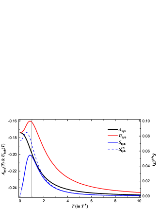
Figure 1: The hybridization free–energy $A_{\rm hyb}$ (in unit of $\Delta$) and the hybridization entropy $S_{\rm hyb}$ (in unit of $k_{\mbox{\tiny B}}$). We set $\varepsilon=0.5\Delta$, $\gamma=4\Delta$ and $\eta=0.5\Delta$. Temperature $T$ is in unit of $T^{\ast}$, Eq. (44). See text for the details.

Figure 1 depicts the resultant hybridization free–energy $A_{\rm hyb}(T)$ (black), internal energy $U_{\rm hyb}(T)$ (blue) and entropy $S_{\rm hyb}(T)$ (red). The observations and discussions are as follows: (i) $A_{\rm hyb}(T)\leq 0$ that indicates the hybridization is spontaneous. It decreases monotonically and is flat off to the value of $A_{\rm hyb}(T\rightarrow\infty)\approx-0.247\Delta$; (ii) The spontaneous process in study is both energetically and entropically favored, as the observed $U_{\rm hyb}(T)<0$ and $S_{\rm hyb}(T)>0$; (iii) There is a characteristic temperature, $T_{\text{max}}$, at which $U_{\rm hyb}(T)$ reaches its maximum; (iv) It is noticed that for quantum Brownian oscillators that are purely harmonic, neither $U_{\rm hyb}$ nor $S_{\rm hyb}$ exhibits the turnover behaviors.OCo0615 ; Hor057325 ; Hor081161 One can therefore conclude that the observed turnovers in Fig. 1 are an anharmonic characteristic; (v) However, the quantification on $T_{\text{max}}$ is generally complicated. It involves the interplay between the solvent induced reorganization energy, the fluctuation time, and how they effectively participate in the thermodynamic integration. Nevertheless, as inferred from Eq. (42) with Eq. (43), it would be rather reasonable to have $T_{\text{max}}\approx\{[(\varepsilon-\eta/2)^{2}+\Delta^{2}]/\pi\}^{\frac{1}{2}}$; (vi) Adopt for the unit of temperature in Fig. 1 rather a bare–system property,

$$T^{\ast}=\frac{2}{\tau^{\ast}},\ \ \,\text{with}\ \ \,\tau^{\ast}\equiv\frac{2\pi}{\Omega_{\mbox{\tiny S}}}=\frac{2\pi}{2\sqrt{\varepsilon^{2}+\Delta^{2}}}.$$ (44)

Here, $\Omega_{\mbox{\tiny S}}\equiv 2\sqrt{\varepsilon^{2}+\Delta^{2}}$ is the characteristic frequency of the bare two–level $\hat{H}_{\mbox{\tiny S}}$ of Eq. (42); thus, $\tau^{\ast}\equiv 2\pi/\Omega_{\mbox{\tiny S}}$ denotes the periodic time. The corresponding imaginary time analog is then $1/T^{\ast}=\tau^{\ast}/2$. In fact, $T^{\ast}$ does nicely locate the maximum on the local–energy difference, $E^{\rm hyb}_{\mbox{\tiny S}}(T)\equiv{\rm tr}_{\mbox{\tiny S}}[\hat{H}_{\mbox{\tiny S}}\rho^{\rm eq}_{\mbox{\tiny S}}(T)]-{\rm tr}_{\mbox{\tiny S}}[\hat{H}_{\mbox{\tiny S}}\rho^{\rm eq}_{\mbox{\tiny S};\lambda=0}(T)]$, where $\rho^{\rm eq}_{\mbox{\tiny S};\lambda=0}(T)$ is the unmixed counterpart to $\rho^{\rm eq}_{\mbox{\tiny S}}(T)$; (vii) In general, $E^{\rm hyd}_{\mbox{\tiny S}}(T)\neq U_{\rm hyb}(T)$ and their maximum temperatures, $T^{\ast}$ and $T_{\rm max}$, are also different. The thermalization underlying the internal energy $U_{\rm hyb}(T)$ is rather complicated, as mentioned early. The sign of $T_{\rm max}-T^{\ast}$ can be either positive or negative [not shown here but would have been implied in (v) above].

Included in Fig. 1 is also the von Neumann entropy counterpart (dash–blue),

$$S^{\rm vN}_{\rm hyb}(T)\equiv S_{\text{vN}}[\rho^{\rm eq}_{\mbox{\tiny S}}(T)]-S_{\text{vN}}[\rho^{\rm eq}_{\mbox{\tiny S};0}(T)],$$ (45)

with $S_{\text{vN}}[\rho]\equiv-k_{B}{\rm tr}_{\mbox{\tiny S}}(\rho\ln\rho)$. This is evaluated at the reduced system density operator in the mixture at equilibrium, $\rho^{\rm eq}_{\mbox{\tiny S}}(T)$, versus its unmixed counterpart, $\rho^{\rm eq}_{\mbox{\tiny S};\lambda=0}(T)$. It is observed that

$$S_{\rm hyb}(T)\leq S^{\text{vN}}_{\rm hyb}(T).$$ (46)

While the equal sign holds only for either isolated systems or the $T\rightarrow\infty$ limit, the inequality is general, regardless whether there is anharmonicity or not.OCo0615 ; Hor057325 ; Hor081161 The physical picture is as follows. In contrast to the thermodynamic entropy, the von Neumann entropy engages the reduced description, using only $\rho^{\rm eq}_{\mbox{\tiny S}}(T)={\rm tr}_{\mbox{\tiny B}}\rho^{\rm eq}_{\mbox{\tiny T}}(T)$. This local system property alone contains little information on the system–and–bath entanglement. The loss of mutual information is responsible for the fact that $S_{\text{vN}}(T)$ is always greater than the thermodynamic entropy. The reduced system density operator $\rho^{\rm eq}_{\mbox{\tiny S}}(T)$ intrinsically describes a mixed–state property even at $T=0$. Consequently, $S_{\text{vN}}(T=0)>0$, due to the aforementioned information loss. On the other hand, $S_{\rm hyb}(T\rightarrow 0)=0$, as anticipated via the Third Law of Thermodynamics. Nevertheless, the DEOM–evaluation remains challenge in the zero–temperature limit and the dot–part of the $S_{\rm hyb}(T)$ curve in Fig. 1 is an extrapolation.

By far we have exploited the equilibrium DDOs, $\{\bar{\rho}^{(n)}_{\bf n}(T;\lambda)\}$ of Eq. (38), and evaluated the hybridization free–energy, $A_{\rm hyb}(T)$, Eq. (36) with Eq. (37). It is noticed that the imaginary–time HEOM formalism for ${\rm tr}_{\mbox{\tiny B}}e^{-\tau H_{\mbox{\tiny T}}}/{\rm tr}_{\mbox{\tiny B}}e^{-\beta h_{\mbox{\tiny B}}}$ had been constructed by Tanimura.Tan14044114 ; Tan15144110 Reported there were also for a spin–boson complex the numerically accurate $U_{\text{hyb}}(T)+U^{\mbox{\tiny S}}_{0}(T)$ and $S_{\text{hyb}}(T)+S^{\mbox{\tiny S}}_{0}(T)$. Here, $U^{\mbox{\tiny S}}_{0}(T)={\rm tr}_{\mbox{\tiny S}}[\hat{H}_{\mbox{\tiny S}}\rho^{\rm eq}_{\mbox{\tiny S};\lambda=0}(T)]$ and $S^{\mbox{\tiny S}}_{0}(T)=S_{\text{vN}}[\rho^{\rm eq}_{\mbox{\tiny S};0}(T)]$ are the unmixed bare–system contributions. None of the above two sum–quantities shows turnover behavior. Nevertheless, the above type of quantities does not describe the thermodynamic isotherm process in a closed system, whereas the hybridization part does. It would be prefer to have the imaginary–time DEOM for the hybridization partition function; see Appendix B.

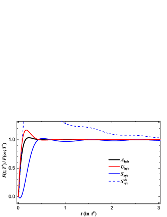
Figure 2: The transient thermodynamics of the spin-boson model of Fig. 1, at $T=T^{\ast}$. Each of them is scaled by its own $F(t\rightarrow\infty)=F^{\rm eq}$, with $(A^{\rm eq}_{\rm hyb},U^{\rm eq}_{\rm hyb})/\Delta=(-0.199,-0.161)$ and $(S^{\rm eq}_{\rm hyb},S^{\rm vN;eq}_{\rm hyb})/k_{\mbox{\tiny B}}=(0.053,0.070)$, respectively.

As mentioned to the end of Sec. IV.2, we can extend the real–time DEOM–evaluation to the transient $A_{\rm hyb}(t;T)$. Moreover, let us treat $A\equiv U-TS$ as the mathematical definition. Together with $S=-(\partial A/\partial T)$, we will recover all involving equilibrium thermodynamic values when $t\rightarrow\infty$. Figure 2 reports the resultant time–dependent functions, $F(t)/F(\infty)$, for the same four physical quantities in Fig. 1 at $T=T^{\ast}$. The total composite system was initially $(t<0)$ in the unhybridized equilibrium state, prior to the switch on of $H_{\mbox{\tiny SB}}$. The reported time $t$ is in unit of $\tau^{\ast}$ [Eq. (44)] that denotes the oscillatory period of the bare system. The observations and discussions are as follows: (i) $A_{\rm hyb}(t;T)\leq 0$ would imply its applicability to the characterization of spontaneous processes that in principle evolve in time; (ii) Physically, the internal energy is a time–dependent variable. It together with (i) would further imply that $A_{\rm hyb}\equiv U_{\rm hyb}-TS_{\rm hyb}$ and $S_{\rm hyb}=-(\partial A_{\rm hyb}/\partial T)$ remain valid for transient processes; (iii) It is known that in a thermodynamics closed system, the entropy change, $S_{\rm hyb}=-(\partial A_{\rm hyb}/\partial T)$, can be either positive or negative. The observed $S_{\rm hyb}(t)<0$ in the short–time region may indicate the formation of a “solvent–cage” surrounding the local two–level impurity in study. The normal thermalization becomes dominant afterward, resulting in $S_{\rm hyb}(t>t_{\text{cage}})>0$. The observed oscillatory behavior is purely dynamics in nature; (iv) In contrast, the von-Neumann entropy $S^{\text{vN}}_{\rm hyb}$ is an information measure, which is always nonnegative. The inequality $S_{\rm hyb}(t;T)<S^{\text{vN}}_{\rm hyb}(t;T)$ remains true in the time–dependent scenario, following the same discussions on Eq. (46).

VI Concluding remarks

In summary, we have presented a comprehensive account on a unified DEOM theory, followed by its accurate evaluations on both the equilibrium and transient thermodynamics functions. Our results are applicable to for arbitrary systems with Gaussian bath environments. Considered in the unified DEOM theory is a class of polynomial–exponential bath dissipaton decomposition scheme, Eq. (11) or Eq. (16) with Eq. (17). This includes the recently proposed FSD for an efficient sum–over–poles expansion of Bose/Fermi function in the extremely low–temperature regime.Cui19024110 ; Zha20064107 It is worth re-emphasizing that the DEOM theory consists of not only Eq. (III) with Eqs. (29) and (30), but also the phase–space dissipaton algebra.Yan14054105 ; Yan16110306 ; Zha18780 ; Wan20041102 The resultant DEOM–space quantum mechanics does unravel the entangled system–and–bath dynamics.Yan14054105 ; Yan16110306 ; Zha18780 ; Wan20041102 Moreover, as shown in Appendix B, one can exploit the analytical continuation dissipaton technique to the imaginary–time DEOM. This formalism is numerically preferred for equilibrium thermodynamics.

Alternative approach is the system–bath coupling strength $\lambda$–integral formalism, Eq. (36). The involving integrand, Eq. (37), can be accurately evaluated with the real–time DEOM theory. This enables the study of both equilibrium and transient thermodynamics. It is shown that the latter would preserve the standard thermodynamic relations including the spontaneity criterion. Numerically accurate results are exemplified with a model spin–boson mixture in Sec. V. This simple system carries two basic characteristics. One is the anharmonicity and another is the formation of bosonic solvent–cage surrounding the local spin impurity. Interestingly, these two characteristics are signified in the specified equilibrium and transient thermodynamics functions, as reported in Fig. 1 and Fig. 2, respectively.

Data Availability

The data that support the findings of this study are available from the corresponding author upon reasonable request.

Appendix A Steady-state solutions to DEOM

This appendix is concerned with the equilibrium DDOs, $\{\bar{\rho}^{(n)}_{\bf n}(T)\}$ of Eq. (31). These are the steady–state solutions, to the hierarchical dynamics, Eq. (III), with Eqs. (29) and (30). The standard choices for solving high-dimension linear equations are the Krylov subspace methods.Saa03 However, due to the hierarchy structure in study, the preferred choice would be the self–consistent iteration (SCI) method developed by Zhang et al.Zha17044105

For bookkeeping we denote

$$\begin{split}{\cal L}^{(n)}_{\bf n}&\equiv iH^{\times}_{\mbox{\tiny S}}+\sum_{k}n_{k}\gamma_{k},\ \ \ \Lambda_{k}\equiv\gamma_{k}\frac{p_{k}\eta_{k}}{\eta_{k-1}},\\ {\cal A}&\equiv\hat{Q}^{\times}_{\mbox{\tiny S}}\ \ \ \text{and}\ \ \ {\cal C}_{k}\equiv\eta_{k}\hat{Q}^{\mbox{\tiny$>$}}_{\mbox{\tiny S}}-\eta_{\bar{k}}^{\ast}\hat{Q}^{\mbox{\tiny$<$}}_{\mbox{\tiny S}}.\end{split}$$ (47)

By setting $\dot{\rho}^{(n)}_{\bf n}=0$, we obtain

$$0 =-{\cal L}^{(n)}_{\bf n}\bar{\rho}^{(n)}_{\bf n}+\sum_{k}n_{k}\Lambda_{k}\bar{\rho}^{(n)}_{{\bf n}^{+,-}_{k-1,k}}$$

$$\quad-i\sum_{k}{\cal A}\bar{\rho}^{(n+1)}_{{\bf n}_{k}^{+}}-i\sum_{k}\delta_{0p_{k}}n_{k}{\cal C}_{k}\bar{\rho}^{(n-1)}_{{\bf n}_{k}^{-}}.$$ (48)

Introduce an arbitrary parameter $\epsilon>0$ and recast the above expression as

$$\bar{\rho}^{(n)}_{\bf{n}} =\big{(}{\cal L}^{(n)}_{\bf{n}}+\epsilon\big{)}^{-1}\Big{[}\epsilon\bar{\rho}^{(n)}_{\bf{n}}+\sum_{k}n_{k}\Lambda_{k}\bar{\rho}^{(n)}_{{\bf n}^{+,-}_{k-1,k}}$$

$$\quad\ -i\sum_{k}{\cal A}\bar{\rho}^{(n+1)}_{\bf{n_{k}^{+}}}-i\sum_{k}\delta_{0p_{k}}n_{k}{\cal C}_{k}\bar{\rho}^{(n-1)}_{\bf{n_{k}^{-}}}\Big{]}.$$ (49)

This constitutes a blocked Jacobi iteration scheme, using the right-hand-side (rhs) DDOs to update the left-hand-side (lhs) one. The SCI accommodates further the hierarchy structure and the efficient on-the-fly filtering algorithm.Shi09084105 It proceeds recursively with increasing $n$ in each iteration cycle, so that all $\bar{\rho}_{{\bf n}_{k}^{-}}^{(n-1)}$ had just been updated. This feature is also true for some $\bar{\rho}^{(n)}_{{\bf n}^{+,-}_{k-1,k}}$, the new ingredients of this work, since the configurations in each individual $n$–dissipatons subset are also pre-ordered. Each hierarchy iteration cycle starts with the reduced system density matrix $\rho^{\rm eq}_{\mbox{\tiny S}}\equiv\bar{\rho}^{(0)}_{\bf 0}$. This determines also the common scaling parameter for all DDOs in that cycle via the normalization constraint on $\text{tr}_{\mbox{\tiny S}}\rho^{\rm eq}_{\mbox{\tiny S}}=1$.

The SCI converges as long as the diagonal part of $({\cal L}^{(n)}_{\bf n}+\epsilon)$ dominates.Zha17044105 This suggests the lower bound for the SCI relaxation parameter $\epsilon$. Increasing $\epsilon$ will increase the numerical stability, but decrease the convergence speed. For a good balance between accuracy and efficiency, we choose $\epsilon\gtrsim\max(\Omega_{\mbox{\tiny S}},\sqrt{L\eta_{\max}})$, where $\Omega_{\mbox{\tiny S}}$ is the system spectrum span, $\eta_{\max}=\max(|\eta_{1}|,\cdots,|\eta_{K}|)$ and $L$ the level of truncation. The advantages of SCI scheme over the Krylov subspace methods are remarkable.Zha17044105

Appendix B The imaginary–time formalism

In line with $A_{\text{hyb}}$ as defined in Eq. (32), the canonical partition function of the total system–and–bath composite reads $Z_{\mbox{\tiny T}}\equiv{\rm Tr}\,e^{-\beta H_{\mbox{\tiny T}}}=Z_{0}Z_{\text{hyb}}$. Note that $H_{\mbox{\tiny T}}=H_{\mbox{\tiny S}}+h_{\mbox{\tiny B}}+H_{\mbox{\tiny S}\mbox{\tiny B}}$ with $[H_{\mbox{\tiny S}},h_{\mbox{\tiny B}}]=0$. The unhybrid part, $Z_{0}\equiv{\rm Tr}\,e^{-\beta(H_{\mbox{\tiny S}}+h_{\mbox{\tiny B}})}=({\rm tr}_{\mbox{\tiny S}}e^{-\beta H_{\mbox{\tiny S}}})({\rm tr}_{\mbox{\tiny B}}e^{-\beta h_{\mbox{\tiny B}}})\equiv Z^{\mbox{\tiny S}}_{0}Z^{\mbox{\tiny B}}_{0}$, contributes to $A_{0}$ in Eq. (32) and is treated as the reference. The imaginary–time $i$-DEOM to be developed in this appendix focuses on

$${\rm tr}_{\mbox{\tiny S}}\varrho^{(0)}_{\bf 0}(\beta)={\rm Tr}\hat{\varrho}_{\mbox{\tiny T}}(\beta)=Z_{\text{hyb}}=e^{-\beta A_{\rm hyb}}.$$ (50)

Remarkably, the $i$-DDOs, which are the $i$-DEOM dynamical variables, acquire also the generic form of Eq. (24):

$$\varrho^{(n)}_{\bf n}(\tau)={\rm tr}_{\mbox{\tiny B}}\big{[}\big{(}\tilde{f}_{K}^{n_{K}}\cdots\tilde{f}_{1}^{n_{1}}\big{)}^{\circ}\hat{\varrho}_{\mbox{\tiny T}}(\tau)\big{]}.$$ (51)

We will identity the $i$-dissipatons, $\{\tilde{f}_{k}\}$, the underlying dissipaton algebra and the resultant $i$-DEOM formalism. All these can be carried out in parallel to Sec. II and Sec. III, but with the methods of analytical continuation.

Let us start with the total composite $\hat{\varrho}_{\mbox{\tiny T}}(\tau)$ in Eq. (51). In contact with the target Eq. (50), we have

$$\hat{\varrho}_{\mbox{\tiny T}}(\tau)\equiv e^{-\tau H_{\mbox{\tiny T}}}e^{-(\beta-\tau)(H_{\mbox{\tiny S}}+h_{\mbox{\tiny B}})}\big{/}(Z^{\mbox{\tiny S}}_{0}Z^{\mbox{\tiny B}}_{0}).$$ (52)

It satisfies [cf. Eq. (23) for notations]

$$\frac{\mbox{d}}{\mbox{d}\tau}{\hat{\varrho}}_{\mbox{\tiny T}}(\tau)=-\big{(}H^{\times}_{\mbox{\tiny S}}+h^{\times}_{\mbox{\tiny B}}+H^{\mbox{\tiny$>$}}_{\mbox{\tiny S}\mbox{\tiny B}}\big{)}\hat{\varrho}_{\mbox{\tiny T}}(\tau),$$ (53)

where $H_{\mbox{\tiny SB}}=\hat{Q}_{\mbox{\tiny S}}\hat{F}_{\mbox{\tiny B}}$. The corresponding $i$-DDOs dynamic equation is then [cf. Eqs. (III)–(27)]

$$\frac{\mbox{d}}{\mbox{d}\tau}\varrho^{(n)}_{\bf n}(\tau) =-H^{\times}_{\mbox{\tiny S}}\varrho^{(n)}_{\bf n}(\tau)-\varrho^{(n)}_{\bf n}(\tau;h^{\times}_{\mbox{\tiny B}})$$

$$\quad-\hat{Q}_{\mbox{\tiny S}}\varrho^{(n)}_{\bf n}(\tau;\hat{F}_{\mbox{\tiny B}}^{\mbox{\tiny$>$}}),$$ (54)

with $H^{\times}_{\mbox{\tiny S}}\varrho^{(n)}_{\bf n}(\tau)\equiv[H_{\mbox{\tiny S}},\varrho^{(n)}_{\bf n}(\tau)]$ and

$$\begin{split}\varrho^{(n)}_{\bf n}(\tau;h^{\times}_{\mbox{\tiny B}})&\equiv{\rm tr}_{\mbox{\tiny B}}\Big{[}\big{(}\tilde{f}_{K}^{n_{K}}\cdots\tilde{f}_{1}^{n_{1}}\big{)}^{\circ}\hat{h}^{\times}_{\mbox{\tiny B}}\hat{\varrho}_{\mbox{\tiny T}}(\tau)\big{]},\\ \varrho^{(n)}_{\bf n}(\tau;\hat{F}^{\mbox{\tiny$>$}}_{\mbox{\tiny B}})&\equiv{\rm tr}_{\mbox{\tiny B}}\big{[}\big{(}\tilde{f}_{K}^{n_{K}}\cdots\tilde{f}_{1}^{n_{1}}\big{)}^{\circ}\hat{F}^{\mbox{\tiny$>$}}_{\mbox{\tiny B}}\hat{\varrho}_{\mbox{\tiny T}}(\tau)\big{]}.\end{split}$$ (55)

Moreover, $\hat{\varrho}_{\mbox{\tiny T}}(0)=e^{-\beta(H_{\mbox{\tiny S}}+h_{\mbox{\tiny B}})}\big{/}(Z^{\mbox{\tiny S}}_{0}Z^{\mbox{\tiny B}}_{0})$ via Eq. (52). This determines the initial $i$-DDOs the values of

$$\varrho^{(0)}_{\bf 0}(0)=e^{-\beta H_{\mbox{\tiny S}}}/Z^{\mbox{\tiny S}}_{0}\ \ \text{and}\ \ \varrho_{\bf n}^{(n>0)}(0)=0.$$ (56)

It is worth noting that $h^{\times}_{\mbox{\tiny B}}$ denotes the bare–bath $h_{\mbox{\tiny B}}$–commutator action. This validates the required analytical continuation methods by setting $t=-i\tau$ to reach at the final $i$–DEOM formalism. First of all, it acquires

$$\widetilde{F}_{\mbox{\tiny B}}(\tau)\equiv\hat{F}_{\mbox{\tiny B}}(t=-i\tau)=e^{\tau h_{\mbox{\tiny B}}}\hat{F}_{\mbox{\tiny B}}e^{-\tau h_{\mbox{\tiny B}}}.$$ (57)

We have $\langle\widetilde{F}_{\mbox{\tiny B}}(0)\widetilde{F}_{\mbox{\tiny B}}(\tau)\rangle_{\mbox{\tiny B}}=\langle\widetilde{F}_{\mbox{\tiny B}}(-\tau)\widetilde{F}_{\mbox{\tiny B}}(0)\rangle_{\mbox{\tiny B}}$ and also

$$\langle\widetilde{F}_{\mbox{\tiny B}}(\tau)\widetilde{F}_{\mbox{\tiny B}}(0)\rangle_{\mbox{\tiny B}}=\langle\widetilde{F}_{\mbox{\tiny B}}(\beta-\tau)\widetilde{F}_{\mbox{\tiny B}}(0)\rangle_{\mbox{\tiny B}}.$$ (58)

The corresponding Eq. (4) with $t=-i\tau$ readsWei12

$$\langle\widetilde{F}_{\mbox{\tiny B}}(\tau)\widetilde{F}_{\mbox{\tiny B}}(0)\rangle_{\mbox{\tiny B}}=\frac{1}{\pi}\!\int_{-\infty}^{\infty}\!{\rm d}\omega\,\frac{e^{-\tau\omega}J(\omega)}{1-e^{-\beta\omega}}.$$ (59)

This is an analytical function in the required $\tau\in[0,\beta]$. Consequently, the Cauchy’s contour integration technique is applicable. On the other hand, one can recast Eq. (59) as

$$\langle\widetilde{F}_{\mbox{\tiny B}}(\tau)\widetilde{F}_{\mbox{\tiny B}}(0)\rangle_{\mbox{\tiny B}}=\lim_{t\rightarrow 0}\frac{1}{\pi}\!\int_{-\infty}^{\infty}\!{\rm d}\omega\,\frac{e^{-i\omega(t-i\tau)}J(\omega)}{1-e^{-\beta\omega}}.$$

The analytical continuation of Eq. (11) reads then

$$\langle\widetilde{F}_{\mbox{\tiny B}}(\tau)\widetilde{F}_{\mbox{\tiny B}}(0)\rangle_{\mbox{\tiny B}} =\sum_{k=1}^{K}\eta_{k}\phi_{k}(-i\tau),$$ (60a)

$$\langle\widetilde{F}_{\mbox{\tiny B}}(0)\widetilde{F}_{\mbox{\tiny B}}(\tau)\rangle_{\mbox{\tiny B}} =\sum_{k=1}^{K}\eta^{\ast}_{\bar{k}}\phi_{k}(-i\tau),$$ (60b)

with $\phi_{k}(-i\tau)=(-i\gamma_{k}\tau)^{p_{k}}e^{i\gamma_{k}\tau}$, Eq. (16). We have numerically verified that in the limit of $K\rightarrow\infty$, Eq. (60a) agrees perfectly with Eq. (59) where $\tau\in[0,\beta]$. The resultant sum is practically real, which together with $\langle\widetilde{F}_{\mbox{\tiny B}}(0)\widetilde{F}_{\mbox{\tiny B}}(\tau)\rangle_{\mbox{\tiny B}}=\langle\widetilde{F}_{\mbox{\tiny B}}(-\tau)\widetilde{F}_{\mbox{\tiny B}}(0)\rangle_{\mbox{\tiny B}}$ give rise to Eq. (60b). The associate index $\bar{k}$ was defined before after Eq. (6). To reproduce Eq. (60), we identify [cf. Eqs. (18) and (19)]

$$\hat{F}_{\mbox{\tiny B}} =\sum_{k=1}^{K}\tilde{f}_{k},$$ (61)

with

$$\begin{split}\langle\tilde{f}_{k}(\tau)\tilde{f}_{j}(0)\rangle_{\mbox{\tiny B}}&=\delta_{kj}\eta_{k}\phi_{k}(-i\tau),\\ \langle\tilde{f}_{j}(0)\tilde{f}_{k}(\tau)\rangle_{\mbox{\tiny B}}&=\delta_{kj}\eta^{\ast}_{\bar{k}}\phi_{k}(-i\tau).\end{split}$$ (62)

As defined in Eq. (57), $\tilde{f}_{k}(\tau)=e^{\tau h_{\mbox{\tiny B}}}\tilde{f}_{k}e^{-\tau h_{\mbox{\tiny B}}}$ that satisfies $-(\partial\tilde{f}_{k}/\partial\tau)_{\mbox{\tiny B}}=[\hat{f}_{\mbox{\tiny B}},\hat{h}_{\mbox{\tiny B}}]$. We obtain [cf. Eq. (30)]

$$\varrho_{\bf n}^{(n)}(\tau;h^{\times}_{\mbox{\tiny B}})=i\sum_{k}n_{k}\gamma_{k}\bigg{[}\frac{p_{k}\eta_{k}}{\eta_{k-1}}\varrho^{(n)}_{{\bf n}^{+,-}_{k-1,k}}\!(\tau)-\varrho^{(n)}_{\bf n}(\tau)\bigg{]},$$

and also [cf. Eq. (29)]

$$\varrho^{(n)}_{\bf n}(\tau;\hat{F}^{\mbox{\tiny$>$}}_{\mbox{\tiny B}})=\sum_{k}\left[\varrho^{(n+1)}_{{\bf n}_{k}^{+}}(\tau)+\delta_{0p_{k}}n_{k}\eta_{k}\varrho^{(n-1)}_{{\bf n}^{-}_{k}}(\tau)\right].$$

Both are identical to their real–time counterparts. All parameters are identical to to those specified in Sec. II.2. The resultant Eq. (B) reads [cf. Eqs. (47) and (A)]

$$\frac{\mbox{d}\varrho^{(n)}_{\bf n}}{\mbox{d}\tau} =i{\cal L}^{(n)}_{\bf n}\varrho^{(n)}_{\bf n}-i\sum_{k}n_{k}\Lambda_{k}\varrho^{(n)}_{{\bf n}^{+,-}_{k-1,k}}$$

$$\quad-\hat{Q}_{\mbox{\tiny S}}\sum_{k}\left(\varrho^{(n+1)}_{{\bf n}_{k}^{+}}+\delta_{0p_{k}}n_{k}\eta_{k}\varrho^{(n-1)}_{{\bf n}^{-}_{k}}\right).$$ (63)

This is the unified $i$-DEOM formalism of this work, with the initial values of Eq. (56) to be propagated to $\{\varrho^{(n)}_{\bf n}(\tau=\beta);n=0,\cdots,L\}$. Together with Eq. (50), we can evaluate $A_{\rm hyb}(T)$ without invoking the $\lambda$–integration as Eq. (36). Moreover, the above $i$-dissipaton formalism goes with a one–to–one correspondence manner, such as Eq. (51) versus Eq. (24) and Eq. (19) versus Eq. (62), respectively. As results,

$$\bar{\rho}^{(n)}_{\bf n}(T)=\frac{\varrho^{(n)}_{\bf n}(\beta)}{Z_{\text{hyb}}}=\frac{\varrho^{(n)}_{\bf n}(\beta)}{{\rm tr}_{\mbox{\tiny S}}\varrho^{(0)}_{\bf 0}(\beta)}.$$ (64)

This is an alternative approach to the equilibrium DDOs, Eq. (31) or Eq. (A).

References

• (1) B. L. Hu, J. P. Paz, and Y. Zhang, Phys. Rev. D 45, 2843 (1992).
• (2) R. X. Xu, B. L. Tian, J. Xu, and Y. J. Yan, J. Chem. Phys. 130, 074107 (2009).
• (3) A. O. Caldeira and A. J. Leggett, Ann. Phys. 149, 374 (1983), [Erratum: 153, 445 (1984)].
• (4) H. Grabert, U. Weiss, and P. Talkner, Z. Phys. B Condens. Matter 55, 87 (1984).
• (5) H. Grabert, P. Schramm, and G. L. Ingold, Phys. Rep. 168, 115 (1988).
• (6) C. Hörhammer and H. Büttner, J. Phys. A. Math. Gen. 38, 7325 (2005).
• (7) C. Hörhammer and H. Büttner, J. Stat. Phys. 133, 1161 (2008).
• (8) R. F. O’Connell, J. Stat. Phys. 124, 15 (2006).
• (9) M. Campisi, P. Talkner, and P. Hänggi, J. Phys. A: Math. Theor. 42, 392002 (2009).
• (10) R. P. Feynman and F. L. Vernon, Jr., Ann. Phys. 24, 118 (1963).
• (11) Y. Tanimura and R. Kubo, J. Phys. Soc. Jpn. 58, 101 (1989).
• (12) Y. Tanimura, Phys. Rev. A 41, 6676 (1990).
• (13) Y. Tanimura, J. Phys. Soc. Jpn. 75, 082001 (2006).
• (14) Y. A. Yan, F. Yang, Y. Liu, and J. S. Shao, Chem. Phys. Lett. 395, 216 (2004).
• (15) R. X. Xu, P. Cui, X. Q. Li, Y. Mo, and Y. J. Yan, J. Chem. Phys. 122, 041103 (2005).
• (16) R. X. Xu and Y. J. Yan, Phys. Rev. E 75, 031107 (2007).
• (17) Y. Tanimura, J. Chem. Phys. 141, 044114 (2014).
• (18) Y. Tanimura, J. Chem. Phys. 142, 144110 (2015).
• (19) Y. J. Yan, J. Chem. Phys. 140, 054105 (2014).
• (20) Y. J. Yan, J. S. Jin, R. X. Xu, and X. Zheng, Frontiers Phys. 11, 110306 (2016).
• (21) H. D. Zhang, R. X. Xu, X. Zheng, and Y. J. Yan, Mol. Phys. 116, 780 (2018), Special Issue, “Molecular Physics in China”.
• (22) Y. Wang, R. X. Xu, and Y. J. Yan, J. Chem. Phys. 152, 041102 (2020).
• (23) H. D. Zhang, R. X. Xu, X. Zheng, and Y. J. Yan, J. Chem. Phys. 142, 024112 (2015).
• (24) H. D. Zhang, Q. Qiao, R. X. Xu, and Y. J. Yan, J. Chem. Phys. 145, 204109 (2016).
• (25) J. S. Jin, S. K. Wang, X. Zheng, and Y. J. Yan, J. Chem. Phys. 142, 234108 (2015).
• (26) J. S. Jin, S. K. Wang, J. H. Zhou, W. M. Zhang, and Y. J. Yan, New. J. Phys. 20, 043043 (2018).
• (27) J. S. Jin, Phys. Rev. B 101, 235144 (2020).
• (28) L. Cui, H. D. Zhang, X. Zheng, R. X. Xu, and Y. J. Yan, J. Chem. Phys. 151, 024110 (2019).
• (29) H. D. Zhang, L. Cui, H. Gong, R. X. Xu, X. Zheng, and Y. J. Yan, J. Chem. Phys. 152, 064107 (2020).
• (30) J. G. Kirkwood, J. Chem. Phys. 3, 300 (1935).
• (31) R. C. Shuela and E. R. Muller, Phys. Stat. Sol. (b) 43, 413 (1971).
• (32) R. van Zon, L. Hernández de la Peña, G. H. Peslherbe, and J. Schofield, Phys. Rev. E 78, 041103 (2008).
• (33) R. van Zon, L. Hernández de la Peña, G. H. Peslherbe, and J. Schofield, Phys. Rev. E 78, 041104 (2008).
• (34) U. Weiss, Quantum Dissipative Systems, World Scientific, Singapore, 2012, 4rd ed.
• (35) Y. J. Yan and R. X. Xu, Annu. Rev. Phys. Chem. 56, 187 (2005).
• (36) X. Zheng, R. X. Xu, J. Xu, J. S. Jin, J. Hu, and Y. J. Yan, Prog. Chem. 24, 1129 (2012).
• (37) R. X. Xu, Y. Liu, H. D. Zhang, and Y. J. Yan, J. Chem. Phys. 148, 114103 (2018).
• (38) Y. Liu, R. X. Xu, H. D. Zhang, and Y. J. Yan, Chin. J. Chem. Phys. 31, 245 (2018).
• (39) J. Hu, R. X. Xu, and Y. J. Yan, J. Chem. Phys. 133, 101106 (2010).
• (40) J. Hu, M. Luo, F. Jiang, R. X. Xu, and Y. J. Yan, J. Chem. Phys. 134, 244106 (2011).
• (41) J. J. Ding, R. X. Xu, and Y. J. Yan, J. Chem. Phys. 136, 224103 (2012).
• (42) J. J. Ding, H. D. Zhang, Y. Wang, R. X. Xu, X. Zheng, and Y. J. Yan, J. Chem. Phys. 145, 204110 (2016).
• (43) Z. F. Tang, X. L. Ouyang, Z. H. Gong, H. B. Wang, and J. L. Wu, J. Chem. Phys. 143, 224112 (2015).
• (44) C. R. Duan, Z. F. Tang, J. S. Cao, and J. L. Wu, Phys. Rev. B 95, 214308 (2017).
• (45) J. J. Ding, Y. Wang, H. D. Zhang, R. X. Xu, X. Zheng, and Y. J. Yan, J. Chem. Phys. 146, 024104 (2017).
• (46) L. Z. Ye, H. D. Zhang, Y. Wang, X. Zheng, and Y. J. Yan, J. Chem. Phys. 147, 074111 (2017).
• (47) H. D. Zhang, Q. Qiao, R. X. Xu, X. Zheng, and Y. J. Yan, J. Chem. Phys. 147, 044105 (2017).
• (48) J. C. Phillips, R. Braun, W. Wang, J. Gumbart, E. Tajkhorshid, E. Villa, C. Chipot, R. D. Skeel, L. Kalé, and K. Schulten, J. Comput. Chem. 26, 1781 (2005).
• (49) R. Salomon-Ferrer, D. A. Case, and R. C. Walker, Wiley Interdisciplinary Reviews: Comput. Mol. Sci. 3, 198 (2013).
• (50) M. J. Abraham, T. Murtola, R. Schulz, S. Pall, J. C. Smith, B. Hess, and E. Lindahl, SoftwareX 1-2, 19 (2015).
• (51) J. E. Hirsch and R. M. Fye, Phys. Rev. Lett. 56, 2521 (1986).
• (52) E. Gull, A. J. Millis, A. I. Lichtenstein, A. N. Rubtsov, M. Troyer, and P. Werner, Rev. Mod. Phys. 83, 349 (2011).
• (53) S. R. White, Phys. Rev. Lett. 69, 2863 (1992).
• (54) G. Vidal, Phys. Rev. Lett. 91, 147902 (2003).
• (55) K. G. Wilson, Rev. Mod. Phys. 47, 773 (1975).
• (56) R. Bulla, T. A. Costi, and T. Pruschke, Rev. Mod. Phys. 80, 395 (2008).
• (57) Y. Saad, Iterative Methods for Sparse Linear Systems, Society for Industrial and Applied Mathematics, xx, 2nd edition, 2003.
• (58) Q. Shi, L. P. Chen, G. J. Nan, R. X. Xu, and Y. J. Yan, J. Chem. Phys. 130, 084105 (2009).