Shortcuts to Adiabaticity for the Quantum Rabi Model: Efficient Generation of Giant Entangled cat States via Parametric Amplification

Abstract

We propose a method for the fast generation of nonclassical ground states of the Rabi model in the ultrastrong and deep-strong coupling regimes via the shortcuts-to-adiabatic (STA) dynamics. The time-dependent quantum Rabi model is simulated by applying parametric amplification to the Jaynes-Cummings model. Using experimentally feasible parametric drive, this STA protocol can generate large-size Schrödinger cat states, through a process that is $\sim 10$ times faster compared to adiabatic protocols. Such fast evolution increases the robustness of our protocol against dissipation. Our method enables one to freely design the parametric drive, so that the target state can be generated in the lab frame. A largely detuned light-matter coupling makes the protocol robust against imperfections of the operation times in experiments.

Introduction.—The quantum Rabi model Rabi (1936, 1937); Braak (2011) is the lowest-dimensional Hamiltonian describing the light-matter interaction beyond the rotating-wave approximation (RWA),

$${H}_{\rm{R}}=\omega_{c}{a}^{{\dagger}}{a}+\frac{\omega_{q}}{2}{\sigma}_{z}+{\sigma}_{x}(g{a}^{{\dagger}}+g^{*}{a}).\ \ \ \ \ (\hbar=1)$$ (1)

Here, $\omega_{c}$ $(\omega_{q})$ is the frequency of the cavity (qubit), $g$ is the light-matter coupling strength, ${a}^{{\dagger}}$ (${a}$) is the creation (annihilation) operator of the cavity field, and ${\sigma}_{x}$ and ${\sigma}_{z}$ are Pauli operators of the qubit. This model was first introduced 90 years ago and it has been used to describe the dynamics of a wide variety of physical setups Auffèves et al. (2013), ranging from quantum optics to condensed matter physics. The popular models of Dicke Dicke (1954), Hopfield Hopfield (1958), and Tavis-Cummings Tavis and Cummings (1968) are just multiqubit generalizations of the Rabi model, while the Jaynes-Cummings (JC) model Jaynes and Cummings (1963) is its simplified version Kockum et al. (2019). Generally, the Rabi model can be divided into different coupling regimes Kockum et al. (2019); Forn-Díaz et al. (2019); Rossatto et al. (2017), according to the normalized coupling strength $\eta=g/\omega_{c}$. When focusing on the ultrastrong ($|\eta|\simeq 0.1\sim 1$) and deep-strong ($|\eta|\gtrsim 1$) regimes, the counterrotating terms in ${H}_{\rm{R}}$ cannot be neglected. This leads to areas of unexplored physics and gives rise to many fascinating quantum phenomena, such as the asymmetry of vacuum Rabi splitting Cao et al. (2011), nonclassical photon statistics Ashhab (2013); Ashhab and Nori (2010), and superradiance transition Ridolfo et al. (2012, 2013); Shammah et al. (2017, 2018).

For instance, the ground state of the Rabi model is a squeezed-vacuum state and involves virtual cavity photons Ashhab and Nori (2010); Hines et al. (2004); Leroux et al. (2017). Specifically, when $\omega_{q}\ll g$, the ground state of the Rabi model is

$$|G\rangle= \frac{1}{2}\left(\mathcal{N}_{+}|g\rangle|\text{cat}_{+}\rangle-\mathcal{N}_{-}|e\rangle|\text{cat}_{-}\rangle\right),$$ (2)

which is an entangled Schrödinger cat state. Here, $\mathcal{N}_{\pm}=\sqrt{2\left[1\pm\exp{\left(-2|\eta|^{2}\right)}\right]}$ determine the probability amplitudes of the even ($+$) and odd ($-$) cat states $|\text{cat}_{\pm}\rangle=(|\eta\rangle\pm|-\eta\rangle)/\mathcal{N}_{\pm}$, respectively. The states $|\pm\eta\rangle$ are coherent states. The state $|g\rangle$ $(|e\rangle)$ is the ground (excited) state of the qubit. By imposing the system to be in this ground state, one can generate the maximally entangled cat state (MECS) when $\mathcal{N}_{+}\simeq\mathcal{N}_{-}$. The generation of the MECSs is significant not only for the demonstration of the fundamentals of quantum physics, but also has wide applications in modern quantum technologies, such as quantum information processing Hacker et al. (2019); Li et al. (2017); Mirrahimi et al. (2014); Albert et al. (2016); Huang et al. (2020) and quantum metrology Joo et al. (2011). For instance, giant cat qubits are very robust against photon dephasing, so that they can be very promising for fault-tolerant quantum computation Li et al. (2017); Mirrahimi et al. (2014); Albert et al. (2016).

To generate the MECS, the system needs to enter the deep-strong coupling (DSC) regime of $|\eta|\gtrsim\sqrt{2}$, which is, however, still difficult to achieve in experiments Niemczyk et al. (2010); Forn-Díaz et al. (2010); Bosman et al. (2017); Forn-Díaz et al. (2016a); Yoshihara et al. (2016); Forn-Díaz et al. (2016b); Baust et al. (2016); Chen et al. (2017a); Yoshihara et al. (2017, 2018). Researchers are encouraged to use simulation protocols Ballester et al. (2012); Mezzacapo et al. (2014); Sánchez Muñoz et al. (2020); Langford et al. (2017); Qin et al. (2018); Leroux et al. (2018); Lü et al. (2015); Chen et al. (2019); Burd et al. (2019); Arenz et al. (2020); Burd et al. (2020); Qin et al. (2020) based on the JC model Shore and Knight (1993); Scully and Zubairy (1997); Agarwal (2009) to study exotic phenomena in the DSC regime. For instance, using linear Ballester et al. (2012) or nonlinear drives Qin et al. (2018); Leroux et al. (2018), one can modify the sideband of a cavity-qubit coupled system, so as to enhance the effective light-matter coupling to enter the DSC regime. This opens the possibility to adiabatically control the effective coupling strength based on, e.g., a time-dependent parametric drive, to prepare the target state $|G\rangle$ in the squeezed-light frame Leroux et al. (2018). However, the adiabatic control requires a very small changing rate in the control parameters, usually leading to a long-time evolution. Such a long-time evolution inevitably increases the effect of dissipation, resulting in a low-fidelity target state. In addition, how to turn off the parametric drive without affecting the prepared entangled state is still an open problem.

In this Letter, we propose to use shortcuts-to-adiabatic (STA) methods Guéry-Odelin et al. (2019); Torrontegui et al. (2013); Chen et al. (2010a); Demirplak and Rice (2003); Berry (2009); Chen et al. (2010b); del Campo (2013); Baksic et al. (2016); Chen et al. (2016a); Zhang et al. (2017); Chen et al. (2016b); Ji et al. (2019), e.g., counterdiabatic (CD) driving, to rapidly generate the target state $|G\rangle$. The STA methods are a series of protocols mimicking adiabatic dynamics beyond the adiabatic limit and have been widely applied for quantum state engineering Emmanouilidou et al. (2000); del Campo et al. (2012); Abah et al. (2020); Saberi et al. (2014); Chen et al. (2017b); Hatomura (2018); Ibáñez et al. (2012); Puri et al. (2017); Funo et al. (2020); Du et al. (2016); Zhou et al. (2016); Vepsäläinen et al. (2019); Kölbl et al. (2019); Campbell et al. (2015); Lemonde et al. (2016); Hegade et al. (2020). Specifically, the CD driving Demirplak and Rice (2003); Berry (2009) enables controlling a quantum system, such that the system can accurately evolve along an adiabatic path (e.g., an instantaneous eigenstate of the reference Hamiltonian) beyond the adiabatic limit, where nonadiabatic excitations can be precisely compensated by, e.g., adding an auxiliary driving term to a reference Hamiltonian Kolodrubetz et al. (2017). Using the STA method allows us to significantly shorten the evolution time as compared to the adiabatic protocol. Thus, we can suppress the effect of dissipation and significantly improve the fidelity of a given state. The parametric drive can be smoothly turned off in our STA protocol, because the amplitudes of the parametric drive are continuously turnable. Additionally, the discussed model is generic, so our proposal can be realized in many physical systems, in particular, circuit quantum electrodynamics (QED) systems Qin et al. (2018); Leroux et al. (2018); Lemonde et al. (2016) or ion traps Burd et al. (2019, 2020).

Adiabatic limit.—Assuming $\omega_{q}\ll g$ and $H_{\rm{R}}\equiv H_{\rm{R}}(t)$ [with a controllable parameter $\eta\equiv\eta(t)$] to be time dependent, the Rabi Hamiltonian in Eq. (1) can be diagonalized by the unitary operator Kockum et al. (2019); Forn-Díaz et al. (2019)

$${U}(t)=|{+_{x}}\rangle\langle{+_{x}}|{D}[-\eta(t)]+|{-_{x}}\rangle\langle{-_{x}}|{D}[\eta(t)],$$ (3)

where $|\pm_{x}\rangle$ are the eigenstates of $\sigma_{x}$ and ${D}[\eta(t)]=\exp[\eta(t){a}^{{\dagger}}-\eta^{*}(t){a}]$ is the displacement operator. To avoid the nonadiabatic transitions between the instantaneous eigenstates $\{|E_{m}(t)\rangle\}$ [eigenvalues $\xi_{m}(t)$] of $H_{\rm{R}}(t)$, the system needs to satisfy the adiabatic condition $|\langle E_{m}(t)|\dot{E}_{n\neq m}(t)\rangle|\ll|\xi_{m}(t)-\xi_{n}(t)|$.

CD-driving Hamiltonian.—According to Eq. (3) and Berry’s transitionless algorithm Berry (2009), the CD-driving Hamiltonian for the reference Hamiltonian $H_{\rm{R}}(t)$ is

$${H}_{\rm{CD}}(t)=i\dot{U}(t){U}^{{\dagger}}(t)=i{\sigma}_{x}[\dot{\eta}^{*}(t){a}-\dot{\eta}(t){a}^{{\dagger}}].$$ (4)

The desired STA process can be realized by adding the CD-driving Hamiltonian $H_{\rm{CD}}(t)$ into the reference Hamiltonian $H_{\rm{R}}(t)$ to construct a feasible total Hamiltonian: i.e., $H_{\rm{tot}}(t)=H_{\rm{R}}(t)+H_{\rm{CD}}(t)$ Chen et al. (2010b). In this case, we can predict an ideal evolution along the instantaneous eigenstate $|E_{m}(t)\rangle$, as ${H}_{\rm{tot}}(t)$ ideally satisfies the Schrödinger equation $i|\dot{E}_{m}(t)\rangle=[\xi_{m}(t)+H_{\rm{CD}}(t)]|E_{m}(t)\rangle$ Chen et al. (2017b). Thus, assuming the initial state to be $|E_{0}(0)\rangle=|g\rangle|0\rangle$, we obtain the target state $|E_{0}(t_{f})\rangle=|G\rangle$ at the final time $t_{f}$. However, realizing a time-dependent Rabi model in the DSC regime is still a major challenge in experiments. In the following, we illustrate how to simulate $H_{\rm{tot}}(t)$ based on a parametrically driven JC model, so as to realize the STA protocol and generate the state $|G\rangle$.

Figure 1: Schematic illustration of a cavity QED system containing a single-mode cavity, a qubit, a $\chi^{(2)}$-nonlinear medium, and an optical parametric amplifier (OPA). The qubit ($|g\rangle$=ground state and $|e\rangle$=excited state) coupled to the cavity with coupling strength $\lambda$ and large detuning $\Delta$. The nonlinear drive $\Omega_{\rm{r}}(t)$ induces a time-dependent squeezed-cavity mode. The other nonlinear drive $\Omega_{\rm{i}}(t)$ [$\pi/2$-dephased from $\Omega_{\rm{r}}(t)$] is applied to counteract the nonadiabatic transition induced by mapping the system dynamics into the time-dependent squeezed-light frame. The OPA is used to generate a squeezed-vacuum reservoir, which couples to the cavity mode to minimize the influence of the squeezing-induced noise.

Model and effective Hamiltonian.—As shown in Fig. 1, our STA proposal is realized in the JC model. The cavity is subjected to two time-dependent (two-photon) drives, with the same frequency $\omega_{p}$, but with different real amplitudes, $\Omega_{\rm{r}}(t)$ and $\Omega_{\rm{i}}(t)$. The drive $\Omega_{\rm{i}}(t)$ is $\pi/2$-dephased from $\Omega_{\rm{r}}(t)$. The Hamiltonian in a frame rotating at $\omega_{p}/2$ reads

$${H}_{0}(t)=\Delta{a}^{{\dagger}}{a}-\left[\frac{\Omega_{\rm{r}}(t)+i\Omega_{\rm{i}}(t)}{2}{a}^{2}-\lambda{a^{{\dagger}}}\sigma+\text{h.c.}\right],$$ (5)

where $\Delta=\omega_{c}-\omega_{p}/2$, $\sigma=|g\rangle\langle e|$, $\lambda\ll\omega_{\rm{c}/\rm{q}}$ is the qubit-cavity coupling strength, and we have assumed $\omega_{q}=\omega_{p}$. By performing the unitary transformation ${S}(t)=\exp{[r(t)({a}^{{\dagger}2}-{a}^{2})/2]}$, with $r(t)$ satisfying $\tanh\left[2r(t)\right]=\Omega_{\rm{r}}(t)/\Delta$, we obtain the effective Hamiltonian

$${H}_{S}(t) \approx\Delta\text{sech}{[2r(t)]}a^{{\dagger}}a+\lambda{e^{r(t)}}{\sigma_{x}}(a^{{\dagger}}+a)/2,$$ (6)

where we have neglected the undesired terms by assuming $\Omega_{\rm{i}}(t)=\dot{r}(t)$ and $\lambda\ll\Delta$. The condition $\Omega_{\rm{i}}(t)=\dot{r}(t)$ has been applied according to the transitionless algorithm to counteract the nonadiabatic transition caused by the time-dependent unitary transformation $S(t)$ (see the Supplemental Material SM for details). The effective normalized coupling strength of ${H}_{S}(t)$ is

$$\tilde{\eta}(t)=\frac{{\lambda}}{4\Delta}\left\{\exp{[3{r}(t)]}+\exp{[-{r}(t)]}\right\}.$$ (7)

To show the advantages of our STA protocol, as compared to the adiabatic scheme Leroux et al. (2018), in the following discussion we denote $\tilde{*}$ and $*$ ($*=\eta,\lambda,r,\ldots$) to represent all the parameters in the adiabatic and STA processes, respectively. Here, $\tilde{*}$ and $*$ have the same physical meaning.

Adiabatic protocol.—When $|\dot{\tilde{\eta}}(t)|\ll\Delta\text{sech}\left[2\tilde{r}(t)\right]$, one can achieve the adiabatic evolution along the ground eigenstate of $H_{S}(t)$ Leroux et al. (2018). The adiabatic condition requires $\dot{\tilde{r}}(t)/\Delta\rightarrow 0$, thus leading to slow evolution. Figure 2(a) shows the relationship between the total evolution time $\tilde{T}$ and the logarithmic negativity $\tilde{E}_{N}=\log_{2}||\rho^{\Gamma_{\rm{q}}}||_{1}$ Horodecki et al. (2009) of the adiabatic process. Here, ${\Gamma_{\rm{q}}}$ denotes the partial transpose with respect to the qubit, and $||\cdot||_{1}$ the trace norm. The evolution time $\tilde{T}$ significantly increases when the desired entanglement cost grows. To achieve the MECS with $\tilde{E}_{N}\gtrsim 99.99\%$, one needs $\tilde{T}\gtrsim 200/\Delta$ via the adiabatic process.

According to Eq. (7), a fixed final squeezing parameter $\tilde{r}(t_{f})=\tilde{r}_{\rm{max}}$ is needed to obtain the target state $|G\rangle$. As a result, the MECS only can be prepared in the squeezed-light frame rather than the lab frame, i.e., the final state is $S(t_{f})|G\rangle$. To obtain a MECS in the lab frame, one needs to turn off the parametric drive immediately when $t>t_{f}$. However, rapidly decreasing the squeezing parameter $r(t)$ induces an undesired nonadiabatic transition, which pumps many photons into the cavity in a very short time SM . Then, the final state might be unpredictable.

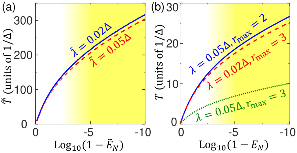
Figure 2: Total evolution time required for (a) the adiabatic process and (b) the STA process, to achieve the MECS versus the desired entanglement cost [characterized by the logarithmic negativity $\tilde{E}_{N}$ ($E_{N}$)]. For (a), the squeezing parameter is $\tilde{r}(t)=\tilde{r}_{\rm{max}}/\{1+\exp{[\tilde{f}(t)]}\}$, where $\tilde{r}_{\rm{max}}$ is the peak value of $\tilde{r}(t)$ and $\tilde{f}(t)=\tilde{f}_{0}(1/2-t/\tilde{T})$, with $\tilde{f}_{0}=10$. For (b), the parameters are $\eta(0)=(1+i)/100$ and ${r}(t)={r}_{\rm{max}}/\{1+\exp{[{f}(t)]}\}$, with $f(t)=f_{0}\cos{(2\pi t/T)}$ and $f_{0}=10$, resulting in $r(0)=r(t_{f})\simeq 0$ and $\dot{r}(0)=\dot{r}(t_{f})\simeq 0$. The light-matter coupling ($\tilde{\lambda},~{}\lambda\ll\Delta$) are chosen to satisfy the condition to neglect the undesired terms to obtain the effective Hamiltonian in Eq. (6). The comparison between the panels shows that, the time required in the STA process to achieve the target state is $\sim 10$ times shorter than that required in the adiabatic process. The yellow-shaded area in each panel shows $(\tilde{E}_{N},\ E_{N}\gtrsim 99\%)$, indicating that the target state in this area is maximally entangled.

STA protocol.—We assume $H_{\rm{tot}}(t)=H_{S}(t)$, resulting in $\Delta\text{sech}[2r(t)]:\Rightarrow\omega_{c}$ and $\lambda\exp{[r(t)]}:\Rightarrow 2[g-i\dot{\eta}(t)]$, where $\eta(t)=g/\omega_{c}$. Thus, we obtain the equations of motion for the coherent state amplitude $\eta(t)$:

$$\text{Re}[\dot{\eta}(t)]= \Delta\text{Im}[\eta(t)]\text{sech}2r(t),$$ (8)

$$\text{Im}[\dot{\eta}(t)]= \frac{\lambda}{2}\exp[{r(t)}]-\Delta\text{Re}[\eta(t)]\text{sech}2r(t),$$ (9)

where $\text{Re}[*]$ ($\text{Im}[*]$) denotes the real (imaginary) part of the parameter “$*$.” Note that $\eta(t)=g/\omega_{c}$ is different from the definition of $\tilde{\eta}(t)$ in Eq. (7), thus the Hamiltonian $H_{S}(t)$ can drive the system to evolve along the ground eigenstate $|E_{0}(t)\rangle$ of the Hamiltonian $H_{\rm{R}}(t)$. According to Eq. (8), $\eta(t)$ relies on the time integration of the squeezing parameter $r(t)$. This allows to rapidly achieve a large value of $\eta(t_{f})$ without any restrictions on the final squeezing parameter $r(t_{f})$. Thus, the STA process can achieve the target state $|G\rangle$ in the lab frame, i.e., $r(t_{f})=0$.

In Fig. 2(b), we display the total evolution time $T$ required for the STA process to obtain the target state versus the logarithmic negativity $E_{N}$. We find that $T$ is significantly shortened when we increase the coupling strength $\lambda$ and the peak squeezing parameter $r_{\rm{max}}$. For an experimentally feasible gain of $10\log_{10}[\exp{(2r_{\rm{max}})}]\sim 20$ dB Clark et al. (2017); Murch et al. (2013); Vahlbruch et al. (2018) (corresponding to $r_{\rm{max}}\sim 2.3$), the evolution time to achieve the MECS with $E_{N}\gtrsim 99.99\%$ via the STA process is $T\sim 20/\Delta$, which is $\sim 10$ times shorter than that via the adiabatic process.

Figure 3: STA protocol when $\eta(0)=(1+i)/100$, $\lambda=0.045\Delta$, and $T=20/\Delta$: (a) Finite-duration drives $\Omega_{\rm{r}}(t)$, $\Omega_{\rm{i}}(t)$ and squeezing parameter $r(t)$ when the peak squeezing parameter $r_{\rm{max}}=2$. (b) Fidelity (the blue vertical axis on the left side) of the target state versus $r_{\rm{max}}$. The red vertical axis on the right side denotes the mean photon number $\bar{n}_{\rm{d}}$ (red-dotted curve with marks “+”) of the target state. The yellow-shaded area in (b) shows $\bar{n}_{\rm{d}}\geq 4$, indicating that the target state in this area can be called a large-size entangled cat state. To generate the large-size entangled cat state with $F\gtrsim 99\%$ and $\bar{n}_{\rm{d}}\simeq 4.3$, one can choose $r_{\rm{max}}=2.3$ (the purple circle).

In the above numerical calculation of Fig. 2(b), we have used the parameter ${r}(t)={r}_{\rm{max}}/\{1+\exp{[{f}(t)]}\}$ with $f(t)=f_{0}\cos{(2\pi t/T)}$, where $f_{0}\gg 1$ controls the initial and final values of the squeezing parameter $r(t)$. With these parameters, the pulses $\Omega_{\rm{r}}(t)$ and $\Omega_{\rm{i}}(t)$ have finite durations, so that we can smoothly turn off the parametric drive [see Fig. 3(a)].

In Fig. 3(b), we show the desired mean photon number $\bar{n}_{\rm{d}}=\langle G|a^{{\dagger}}a|G\rangle$ versus the peak squeezing parameter $r_{\rm{max}}$ (red-dotted curve with “+”). We find that, for a fixed evolution time $T$, $\bar{n}_{\rm{d}}$ increases sharply when $r_{\rm{max}}$ increases. Experimentally, a parametric gain of $\sim 20$ dB ($r_{\rm{max}}\sim 2.3$) has been achieved Burd et al. (2019), and $\sim 30$ dB has also been predicted under experimentally feasible conditions Clark et al. (2017); Murch et al. (2013); Vahlbruch et al. (2018). These realistic parameters allow for generating a high-fidelity ($F>90\%$) target state with $\bar{n}_{\rm{d}}=4\sim 10$ (large-amplitude nonclassical states), as shown by the blue, solid curve in Fig. 3(b). Here, the fidelity of the state $|G\rangle$ is defined as $F=|\langle G|\rho(t_{f})|G\rangle|$. When $r_{\rm{max}}=2.3$ and $\lambda=0.045\Delta$, we find that the target state $|G\rangle$ can be generated with $F\simeq 99\%$ and $\bar{n}_{\rm{d}}\simeq 4$ [see purple circle in Fig. 3(b)].

Robustness of the STA approach—In the following, we focus on discussing the robustness of the STA protocol when $r_{\max}=2.3$ and $\lambda=0.045\Delta$. We first assume the imperfection of a parameter $*$ as $\delta*=*^{\prime}-*$, where $*^{\prime}$ and $*$ denote the actual and ideal values, respectively. Because of large detuning $\lambda\ll\Delta$, when the parametric drive vanishes, the mean photon number and the entanglement of the system can remain unchanged for a long time in the absence of dissipation. Thus, our STA protocol is robust against the imperfect parameters of the total evolution time. As shown in Fig. 4(a), a $20\%$ imperfection of the total evolution time only causes $\lesssim 1\%$ and $\lesssim 5\%$ changes of the logarithmic negativity $E_{N}$ and the mean photon number $\bar{n}_{\rm{d}}$, respectively.

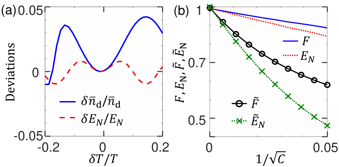
Figure 4: (a) Deviations $\delta\bar{n}_{\rm{d}}$ and $\delta E_{N}$ versus $\delta T$. The STA protocol is robust against the imperfection of the total evolution time $T$. Parameters are the same as in Fig. 3(a). (b) Fidelity $F$ ($\tilde{F}$) and logarithmic negativity $E_{N}$ ($\tilde{E}_{N}$) of the STA (adiabatic) protocol versus $1/\sqrt{C}$. Here, $C=\lambda^{2}/\kappa\gamma$ is the cooperativity, and we assume the dissipation rates $\gamma=\kappa$ for simplicity. The STA and the adiabatic protocols are initially equivalent by assuming $\lambda=\tilde{\lambda}=0.045\Delta$. The total evolution times for the entanglement generation are $T=20/\Delta$ and $\tilde{T}=250/\Delta$, respectively. The squeezing-induced noise is minimized by coupling the cavity to the squeezed-vacuum reservoir SM . As a result, our STA protocol is much more robust against dissipation than the adiabatic protocol.

Then, we compare the entanglement preparation via the STA and the adiabatic processes in the presence of cavity and qubit losses. Because of the relatively strong squeezing, the difference of the frequencies of the photons ($\omega_{p}/2$) pumped by the two-photon drives and those of the squeezed-cavity mode ($\omega_{p}/2+\Delta\text{sech}[2(r(t))]$) is very small, such that the influence of the quantum fluctuation of the photons cannot be ignored. Thus, the two-photon drives may effectively excite the squeezed-cavity mode, so as to induce thermal noise and two-photon correlation noise in the squeezed-cavity mode Qin et al. (2018); Leroux et al. (2018); Lü et al. (2015); Chen et al. (2019). To minimize the influence of such noises, besides accelerating the dynamical evolution Arenz et al. (2020); Burd et al. (2019), one can couple the cavity to a squeezed-vacuum reservoir Ast et al. (2013); Serikawa et al. (2016); Ockeloen-Korppi et al. (2017) with $r_{e}=r_{\rm{max}}$ and $\varphi_{e}=\pi$ during $T/4\lesssim t\lesssim 3T/4$ SM . Here $r_{e}$ and $\varphi_{e}$ are the squeezing parameter and the reference phase of the reservoir, respectively. In this case, the dynamics in the squeezed-light frame can be approximatively described by the standard Lindblad master equation

$$\dot{\rho}_{S}(t)\approx i[\rho_{S}(t),H_{S}(t)]+\gamma\mathcal{D}[\sigma]\rho_{S}(t)+\kappa\mathcal{D}[a]\rho_{S}(t),$$ (10)

where $\mathcal{D}[o]\rho_{S}(t)=o\rho_{S}(t)o^{{\dagger}}-\left[o^{{\dagger}}o\rho_{S}(t)+\rho_{S}(t)o^{{\dagger}}o\right]/2$ is the standard Lindblad superoperator, $\rho_{S}(t)=S^{{\dagger}}(t)\rho(t)S(t)$ is the density operator in the squeezed-light frame, $\gamma$ is the spontaneous emission rate of the qubit, and $\kappa$ is the cavity decay rate.

We define the cooperativity as $C=\lambda^{2}/\kappa\gamma$ and assume $\kappa\simeq\gamma$ for simplicity. By considering the same initial parameters $\lambda=\tilde{\lambda}=0.045\Delta$ and $r(0)=\tilde{r}(0)=0$, we compare the robustness of the STA and that of the adiabatic protocols [see Fig. 4(b)] Johansson et al. (2012). The STA protocol is much more robust against dissipation than the adiabatic scheme, because: (i) the evolution time is significantly shortened in the STA protocol; (ii) the squeezing-induced noise can be well reduced by coupling the cavity to the squeezed-vacuum reservoir in the STA protocol. For experimentally realistic cavity QED parameters: $\Delta/2\pi=1$ GHz, $\lambda/2\pi=45$ MHz, and $\kappa/2\pi=\gamma/2\pi=2.25$ MHz, the STA protocol can achieve the target state with $F\sim 90\%$ and $E_{N}\sim 85\%$, while the adiabatic protocol fails ($\tilde{F}\sim 60\%$ and $\tilde{E}_{N}\sim 45\%$). Then, by measuring the qubit, we can achieve high-fidelity cat states in the lab frame.

Conclusion.—We have investigated how to simulate the STA dynamics of a cavity QED system in the strong coupling regime ($\lambda>\kappa,\gamma$) to prepare a maximally entangled cat state in the lab frame via parametric amplification. A significantly accelerated dynamics ($\sim 10$ times faster than its adiabatic counterpart) makes the system much robust against dissipation. The target state is prepared in a large-detuned JC model, which is driven by finite-duration parametric pulses. Such a setup makes our STA protocol robust against the imperfection of the evolution time. Our proposal is feasible in circuit QED systems, where a transmission line resonator cavity interacts with a superconducting qubit in the JC model Niemczyk et al. (2010); Forn-Díaz et al. (2010); Gu et al. (2017); Xiang et al. (2013). By attaching a superconducting quantum interference device (SQUID) to the end of the resonator Nation et al. (2012); Wallquist et al. (2006); Wang et al. (2019), one can realize a two-photon drive (the Josephson parametric amplification process) by modulating in time the flux through the SQUID. Lemonde et al. (2016); Johansson et al. (2014, 2009); Castellanos-Beltran et al. (2008); Castellanos-Beltran and Lehnert (2007); Johansson et al. (2010); Eichler and Wallraff (2014); Qin et al. (2020). The squeezed vacuum (reservoir) is also produced by Josephson parametric amplifiers, but with a much larger linewidth than that of the cavity Hatridge et al. (2011); Eichler and Wallraff (2014); Castellanos-Beltran and Lehnert (2007); Roy et al. (2015); Mendes et al. (2019); Murch et al. (2013); Toyli et al. (2016). This is possibly the first application of the STA protocols for the Rabi model and we hope that our protocol can find wide applications in studying light-matter interactions, specially, for the ultrastrong and deep-strong coupling regimes Kockum et al. (2019); Forn-Díaz et al. (2019).

Appendix S1 Supplemental Material

In this Supplemental Material, we first discuss the influence of the nonadiabatic transition caused by mapping the system dynamics into the time-dependent squeezed-light frame. Using the transitionless algorithm, we show how to counteract such a nonadiabatic transition with an additional drive, so as to design a shortcuts-to-adiabatic passage to rapidly generate giant entangled cat states. Then, we show how to minimize the influence of the squeezing-induced fluctuation noise by coupling the cavity to a squeezed-vacuum reservoir. Thirdly, we present a possible problem in turning off the parametric drive when the target state is generated in the squeezed-light frame via the adiabatic process.

Appendix S2 S1. Effective Hamiltonian and Dissipation dynamics of the system

S2.1 A. Counteracting the nonadiabatic transition caused by the time-dependent unitary transformation

We begin with a largely detuned Jaynes-Cummings (JC) Hamiltonian driven by a time-dependent parametric (two-photon) drive $\Omega_{r}(t)$,

$${H}_{\rm{1}}(t)=\Delta{a}^{{\dagger}}{a}-\left[\frac{\Omega_{r}(t)}{2}{a}^{2}-\lambda a^{{\dagger}}\sigma+\text{h.c.}\right].$$ (S1)

In the time-dependent squeezed-light frame determined by the squeezing operator $S(t)=\exp{[r(t)({a}^{{\dagger}2}-{a}^{2})/2]}$, with a real squeezing parameter $r(t)$ satisfying $\tanh\left[2r(t)\right]=\Omega_{r}(t)/\Delta$, the Hamiltonian of the system is composed of the following terms:

$$H_{\rm{S1}}(t) =S^{{\dagger}}(t)H_{1}(t)S(t)-iS^{{\dagger}}(t)\dot{S}(t)$$ (S2)

$$={H}_{\rm{S-Rabi}}(t)+H_{\rm{err}}(t)+H_{\rm{NA}}(t),$$ (S3)

$$H_{\rm{S-Rabi}}(t) =\Delta\text{sech}{[2r(t)]}a^{{\dagger}}a+\lambda{\exp{[r(t)]}}{\sigma_{x}}(a^{{\dagger}}+a)/2,$$ (S4)

$$H_{\rm{err}}(t) =-i\lambda{\exp{[-r(t)]}}\sigma_{y}(a^{{\dagger}}-a)/2,$$ (S5)

$$H_{\rm{NA}}(t) =-i\dot{r}(t)(a^{{\dagger}2}-a^{2})/2.$$ (S6)

The Hamiltonian $H_{\rm{S-Rabi}}$ describes the $\sigma_{x}X$ Rabi interaction in the squeezed-light frame, where $X=(a+a^{{\dagger}})/2$ is the canonical position operator. The Hamiltonian $H_{\rm{err}}(t)$ describes the $\sigma_{y}Y$ interaction, where $Y=i(a^{{\dagger}}-a)/2$ is the canonical momentum operator, and can be considered an error term, which can be neglected when $\lambda\ll\Delta$ and $\lambda/\Delta\ll r(t)$. When $r(t)\sim\lambda/\Delta$, the error term $H_{\rm{err}}(t)$ can be neglected by applying a strong drive $\Omega\sigma_{x}$ ($\Omega\gtrsim\Delta$), which induces the coupling of $H_{\rm{err}}(t)$ with a large detuning in the $\sigma_{y}$-direction.

The last term in $H_{\rm{S1}}(t)$, i.e., $H_{\rm{NA}}(t)=-iS^{{\dagger}}(t)\dot{S}(t)$, describes a nonadiabatic transition induced by mapping the system dynamics into the time-dependent squeezed-light frame. It describes the population transfer between different basis in the squeezed-light frame. According to Berry’s transitionless algorithm, we can add a term

$$H_{\rm{SA}}(t)=iS^{{\dagger}}(t)\dot{S}(t)=i\dot{r}(t)(a^{{\dagger}2}-a^{2})/2,$$ (S7)

into the Hamiltonian $H_{\rm{S1}}(t)$ to counteract the nonadiabatic transition. Then, in the laboratory frame, the additional Hamiltonian $H_{\rm{SA}}$ reads

$$H_{\rm{add}}(t)=S(t)H_{\rm{SA}}(t)S^{{\dagger}}=i\dot{r}(t)(a^{{\dagger}2}-a^{2})/2.$$ (S8)

This implies that the cavity mode is subject to another two-photon drive, which has an amplitude $\Omega_{i}(t)=\dot{r}(t)$, a frequency $\omega_{{p}}$, and is $\pi/2$-dephased from $\Omega_{r}(t)$. By adding this additional Hamiltonian $H_{\rm{add}}(t)$ into the Hamiltonian $H_{1}(t)$, we obtain the Hamiltonian $H_{0}(t)$ required for the STA protocol, i.e., the Hamiltonian of Eq. (6) of the main text:

$${H}_{0}(t)=\Delta{a}^{{\dagger}}{a}+\Omega\sigma_{x}-\left[\frac{\Omega_{r}(t)+i\Omega_{i}(t)}{2}{a}^{2}-\lambda{a^{{\dagger}}}\sigma+\text{h.c.}\right].$$ (S9)

Then, we are allowed to rapidly change the squeezing parameter $r(t)$, such that we can quickly adjust the effective qubit-cavity coupling $\lambda\exp{[r(t)]}/2$ in the squeezed-light frame.

This is very important, because applying the STA protocol requires to rapidly change the control parameter, i.e., the normalized coupling strength.

S2.2 B. STA process with parametric drivings

To construct the STA passage, we divide the Hamiltonian $H_{S}(t)$ into two parts:

$$H_{S}(t)=H_{\rm{ref}}(t)+H_{\rm{aux}}(t).$$ (S10)

Here, the Hamiltonian

$$H_{\rm{ref}}(t)=\Delta\text{sech}{[2r(t)]}a^{{\dagger}}a+\sigma_{x}[\chi(t)a^{{\dagger}}+\chi^{*}(t)a],$$ (S11)

is considered as the reference Hamiltonian [with an undetermined parameter $\chi(t)$] for constructing shortcuts,

$$H_{\rm{aux}}(t)=\frac{\lambda{e^{r(t)}}}{2}{\sigma_{x}}(a^{{\dagger}}+a)-\sigma_{x}[\chi(t)a^{{\dagger}}+\chi^{*}(t)a],$$ (S12)

is an auxiliary Hamiltonian. The reference Hamiltonian $H_{\rm{ref}}(t)$ takes the same form as the Rabi Hamiltonian $H_{R}(t)$ [Eq. (1) of the main text], i.e., $H_{\rm{ref}}(t):\Rightarrow H_{R}(t)$, by setting:

$$\omega_{{q}}\ll\omega_{{c}},\ \ \ \omega_{{c}}:\Rightarrow\Delta\text{sech}{[2r(t)]},\ \ \ g:\Rightarrow\chi(t).$$ (S13)

Then, when we choose the parameters to satisfy

$$\eta(t)=\frac{g}{\omega_{c}}=\frac{\chi(t)}{\Delta\text{sech}[2r(t)]},\ \ \ \ \dot{\eta}(t)=\frac{i}{2}\left[{\lambda{e^{r(t)}}}-2\chi(t)\right],$$ (S14)

$H_{\rm{aux}}(t)$ is exactly the CD driving Hamiltonian for the reference Hamiltonian $H_{\rm{ref}}(t)$, i.e., $H_{\rm{aux}}(t):\Rightarrow H_{\rm{CD}}(t)$. Hence, according to the transitionless algorithm, the CD driving Hamiltonian $H_{\rm{aux}}(t)$ can actually drive the system to evolve along an eigenstate of $H_{\rm{ref}}(t)$. The evolution path for our STA protocol is then given as (in the squeezed-light frame)

$$|E_{0}(t)\rangle_{S}=\frac{1}{\sqrt{2}}\left[|+_{x}\rangle|-{\eta}(t)\rangle+|-_{x}\rangle|{\eta}(t)\rangle\right],$$ (S15)

where $|\pm_{x}\rangle$ are the eigenstates of the Pauli matrix $\sigma_{x}$. In the lab frame, the STA evolution path is $S[r(t)]|E_{0}(t)\rangle_{S}$. After some algebra, we can counteract the undetermined parameter $\chi(t)$ and obtain the equations of motion for the coherent state amplitude $\eta(t)$:

$$\text{Re}[\dot{\eta}(t)]= \Delta\text{Im}[\eta(t)]\text{sech}2r(t),$$ (S16)

$$\text{Im}[\dot{\eta}(t)]= \frac{\lambda}{2}\exp[{r(t)}]-\Delta\text{Re}[\eta(t)]\text{sech}2r(t).$$ (S17)

Thus, Eq. (9) of the main text is obtained. The final state in the laboratory frame is

$$S(t_{f})|E_{0}(t_{f})\rangle_{S}=\frac{1}{\sqrt{2}}\left(|+_{x}\rangle|-{\eta}(t_{f})\rangle+|-_{x}\rangle|{\eta}(t_{f})\rangle\right),$$ (S18)

which is an entangled cat state. Here, $S{(t_{f})}=1$ is given according to $r(t_{f})=0$.

S2.3 C. Minimizing the influence of the squeezing-induced fluctuation noise

The Markovian master equation, for a cavity interacting with a broadband squeezed-vacuum reservoir (at zero temperature with squeezing parameter $r_{e}$ and reference phase $\varphi_{e}$), has been well studied (see, e.g., Ref. Scully and Zubairy (1997)). For our STA protocol, when the cavity couples to the squeezed-vacuum reservoir, the master equation in the laboratory frame is

$$\dot{\rho}(t)= i[\rho(t),H_{0}(t)]+\frac{1}{2}\left[2L_{\gamma}\rho(t)L^{{\dagger}}_{\gamma}-L_{\gamma}^{{\dagger}}L_{\gamma}\rho(t)-\rho(t)L_{\gamma}^{{\dagger}}L_{\gamma}\right]$$ (S19)

$$+\frac{1}{2}(N+1)\left[2L_{\kappa}\rho(t)L^{{\dagger}}_{\kappa}-L_{\kappa}^{{\dagger}}L_{\kappa}\rho(t)-\rho(t)L_{\kappa}^{{\dagger}}L_{\kappa}\right]$$ (S20)

$$+\frac{1}{2}N\left[2L_{\kappa}^{{\dagger}}\rho(t)L_{\kappa}-L_{\kappa}L_{\kappa}^{{\dagger}}\rho(t)-\rho(t)L_{\kappa}L_{\kappa}^{{\dagger}}\right]$$ (S21)

$$-\frac{1}{2}M\left[2L_{\kappa}^{{\dagger}}\rho(t)L_{\kappa}^{{\dagger}}-L_{\kappa}^{{\dagger}}L_{\kappa}^{{\dagger}}\rho(t)-\rho(t)L_{\kappa}^{{\dagger}}L_{\kappa}^{{\dagger}}\right]$$ (S22)

$$-\frac{1}{2}M^{*}\left[2L_{\kappa}\rho(t)L_{\kappa}-L_{\kappa}L_{\kappa}\rho(t)-\rho(t)L_{\kappa}L_{\kappa}\right].$$ (S23)

Here, $L_{\gamma}=\sqrt{\gamma}\sigma$ and $L_{\kappa}=\sqrt{\kappa}a$ describe the qubit and cavity decays, with decay rates $\gamma$ and $\kappa$, respectively. The parameters

$$N=\sinh^{2}(r_{e}),\ \ \ \ \text{and}\ \ \ \ M=\cosh{(r_{e})}\sinh{(r_{e})}\exp{(-i\varphi_{e})},$$ (S24)

describe thermal noise and two-photon correlation noise caused by the squeezed-vacuum reservoir, respectively.

Figure S1: Parameters (a) $N_{S}$ and (b) $M_{S}$ characterizing the squeezing-induced noise for $r_{\rm{max}}=2.3$ and $\Omega=0$. Blue-dotted curve in (a) [(b)]: Parameter $N_{S}$ ($M_{S}$) without coupling the cavity to the squeezed-vacuum reservoir (i.e., $r_{e}=0$); Red-solid curve in (a) [(b)]: Parameter $N_{S}$ ($M_{S}$) when the system is coupled to the squeezed-vacuum reservoir during $T/4\lesssim t\lesssim 3T/4$ [i.e., $r_{e}$ is given according to Eq. (S46)]. The yellow-shaded area in (a) or (b) denotes when the cavity is coupled to the squeezed-vacuum reservoir. (c) Fidelities of the ground state $|G\rangle$ versus $1/\sqrt{C}$ calculated by: (blue-dotted curve representing ${F}_{\rm{0}}$) the noise-included master equation in Eq. (S25) when $r_{e}=0$; (red-solid curve representing ${F}$) the noise-included master equation when coupling the cavity to the squeezed-vacuum; (green-dashed curve representing ${F}_{d}$) the effective master equation in Eq. (S48). The parameter $C=\lambda^{2}/\kappa\gamma$ is the cooperativity, and we assume the dissipation rates $\gamma=\kappa$ for simplicity.

By mapping the system dynamics into the time-dependent squeezed-light frame with $S(t)$, the master equation becomes

$$\dot{\rho_{S}}(t)= i[\rho_{S}(t),H_{\rm{S-Rabi}}(t)+H_{\rm{err}}(t)]+\frac{1}{2}\left[2L_{\gamma}\rho_{S}(t)L^{{\dagger}}_{\gamma}-L_{\gamma}^{{\dagger}}L_{\gamma}\rho_{S}(t)-\rho_{S}(t)L_{\gamma}^{{\dagger}}L_{\gamma}\right]$$ (S25)

$$+\frac{1}{2}(N_{S}+1)\left[2L_{\kappa}\rho_{S}(t)L^{{\dagger}}_{\kappa}-L_{\kappa}^{{\dagger}}L_{\kappa}\rho_{S}(t)-\rho_{S}(t)L_{\kappa}^{{\dagger}}L_{\kappa}\right]$$ (S26)

$$+\frac{1}{2}N_{S}\left[2L_{\kappa}^{{\dagger}}\rho_{S}(t)L_{\kappa}-L_{\kappa}L_{\kappa}^{{\dagger}}\rho_{S}(t)-\rho_{S}(t)L_{\kappa}L_{\kappa}^{{\dagger}}\right]$$ (S27)

$$-\frac{1}{2}M_{S}\left[2L_{\kappa}^{{\dagger}}\rho_{S}(t)L_{\kappa}^{{\dagger}}-L_{\kappa}^{{\dagger}}L_{\kappa}^{{\dagger}}\rho_{S}(t)-\rho_{S}(t)L_{\kappa}^{{\dagger}}L_{\kappa}^{{\dagger}}\right]$$ (S28)

$$-\frac{1}{2}M_{S}^{*}\left[2L_{\kappa}\rho_{S}(t)L_{\kappa}-L_{\kappa}L_{\kappa}\rho_{S}(t)-\rho_{S}(t)L_{\kappa}L_{\kappa}\right],$$ (S29)

where $\rho_{S}(t)=S^{{\dagger}}(t)\rho(t)S(t)$ is the density operator of the system in the squeezed-light frame, and

$$N_{S}= \cosh^{2}[r(t)]\sinh^{2}(r_{e})+\sinh^{2}[r(t)]\cosh^{2}(r_{e})+\frac{1}{2}\sinh[2r(t)]\sinh(2r_{e})\cos(\varphi_{e}),$$ (S30)

$$M_{S}= \left\{\sinh[r(t)]\cosh(r_{e})+\exp{(-i\varphi_{e})}\cosh[r(t)]\sinh(r_{e})\right\}$$ (S31)

$$\times\left\{\cosh[r(t)]\cosh(r_{e})+\exp(i\varphi_{e})\sinh[r(t)]\sinh(r_{e})\right\},$$ (S32)

characterize additional noises of the system in the squeezed-light frame. When $r_{e}=0$, $N_{S}$ and $M_{S}$ characterize the squeezing-induced noise. For simplicity, we can assume $\varphi_{e}=\pi$, and obtain

$$N_{S}=\sinh^{2}\left[r_{S}(t)\right],\ \ \ \text{and}\ \ \ M_{S}=\cosh\left[r_{S}(t)\right]\sinh\left[r_{S}(t)\right],$$ (S33)

where $r_{S}(t)=r(t)-r_{e}$. Then, to minimize the parameters $|N_{S}|$ and $|M_{S}|$, we need to minimize the parameter $|r_{S}(t)|$.

Figure S2: blue Fidelities $F$ of the entangled cat state for the STA protocol with $T=20/\Delta$ and $\lambda=0.045\Delta$: (a) [(b)] Fidelity $F$ versus the cooperativity $C$ and the predicted mean photon number $\bar{n}_{d}=|\eta|^{2}$, when the cavity is coupled (decoupled) to the squeezed-vacuum reservoir. For the panels (a) and (b), we choose the squeezing parameter $r_{\rm{max}}\in[0,3]$ corresponding to the $\bar{n}_{d}=|\eta|^{2}\in[0,17]$. (c) Fidelity $F$ versus imperfections of the parameters $r_{e}$ and $T_{e}$. For the panel (c), the squeezing parameter is $r_{\rm{max}}=2.3$.

The waveform of $r\left(t\right)$ of the STA protocol is approximately a square wave when

$${r}(t)=\frac{{r}_{\rm{max}}}{1+\exp{[f_{0}\cos{(2\pi t/T)}]}},$$ (S34)

where $f_{0}=10$ controls the initial and final values of the squeezing parameter $r(t)$. Substituting Eq. (S34) into Eq. (S33) and assuming $r_{e}=0$, in Figs. S1(a) and S1(b), we show the parameters $N_{S}$ and $M_{S}$ describing the squeezing-induced noise (see the blue-dotted curves). As shown, the squeezing-induced noise affects the system dynamics especially when $r(t)$ reaches its maximum value $r_{\rm{max}}$, i.e., $r(t)\approx r_{\rm{max}}$. We accordingly calculate the fidelity $F_{0}=|\langle G|\rho_{S}(t_{f})|G\rangle|$ to show the influence of the squeezing-induced noise [see the blue-dotted curve in Fig. S1(c)]. Here, $|G\rangle$ is the ground state of the Rabi model in the DSC regime [see Eq. (2) of the main text]. The fidelity $F_{0}$ decreases very fast when the dissipation increases.

To minimize the parameter $|r_{S}(t)|$, according to the properties of $\cos(2\pi t/T)$, we can choose

$${r}_{e}=\left\{\begin{array}[]{rcl}0,&&(0\lesssim t\lesssim T/4)\\ \\ r_{\rm{max}},&&(T/4\lesssim t\lesssim 3T/4)\\ \\ 0,&&(3T/4\lesssim t\lesssim T)\end{array}\right.$$ (S40)

i.e., the total interaction time between the cavity and the squeezed-vacuum reservoir is $T_{e}=T/2$, resulting in

$${r}_{S}(t)=\left\{\begin{array}[]{rcl}\displaystyle\frac{{r}_{\rm{max}}}{1+\exp{[f_{0}\cos{(2\pi t/T)}]}},&&(0\lesssim t\lesssim T/4)\\ \\ \displaystyle\frac{-{r}_{\rm{max}}}{1+\exp{[-f_{0}\cos{(2\pi t/T)}]}},&&(T/4\lesssim t\lesssim 3T/4)\\ \\ \displaystyle\frac{{r}_{\rm{max}}}{1+\exp{[f_{0}\cos{(2\pi t/T)}]}}.&&(3T/4\lesssim t\lesssim T)\end{array}\right.$$ (S46)

Then, substituting Eq. (S46) into Eq. (S33), we plot the parameters $N_{S}$ and $M_{S}$ [see the red-solid curves in Fig. S1(a) and S1(b)]. We can accordingly calculate the average values

$$A_{N_{S}}=\frac{1}{T}\int_{0}^{t_{f}}|N_{S}|dt\approx 0.08,\ \ \ \text{and}\ \ \ A_{M_{S}}=\frac{1}{T}\int_{0}^{t_{f}}|M_{S}|dt\approx 0.14,$$ (S47)

which means that the additional noises in Eq. (S25) weakly affect the system dynamics. Thus, the fidelity of the target state $|G\rangle$ is significantly improved [see the red-solid curve in Fig. S1(c)], e.g., from $\sim 65\%$ to $\sim 89\%$ when $1/\sqrt{C}=0.05$. When the desired mean photon number $\bar{n}_{d}$ of the target state increases, the influence of the cavity loss increases [see Figs. S3(a) and S3(b)]. These figures show the fidelities of the target state when the cavity is coupled and decoupled to the squeezed-vacuum reservoir, respectively. According to the comparison between Figs. S1(a) and S1(b), coupling the cavity to the squeezed-vacuum reservoir can effectively suppress the influence of the cavity loss. Thus, the giant ($\bar{n}_{d}\gtrsim 10$) entangled cat states can be generated with a high fidelity. By defining the imperfection of a parameter $*$ as $\delta*=*^{\prime}-*$, the influence of the imperfections of the parameters $T_{e}$ and $r_{e}$ is shown in Fig. S1(c). This figure shows that, slightly decreasing the squeezing parameter $r_{e}$ or increasing the interaction time $T_{e}$ can improve the fidelity $F$. Note that a $10\%$ imperfection of the parameter $r_{e}$ only causes a $3\%$ change in the fidelity, thus the STA protocol is mostly insensitive to the imperfections of the parameter $r_{e}$. When the interaction time $T_{e}$ between the cavity and the squeezed-vacuum reservoir is long enough, our STA protocol is mostly insensitive to the imperfections of the parameter $T_{e}$.

When coupling the cavity to the squeezed-vacuum reservoir during $T/4\lesssim t\lesssim 3T/4$, the evolution can be approximately described by the standard Lindblad master equation

$$\dot{\rho_{S}}(t)\approx i[\rho_{S}(t),H_{\rm{S-Rabi}}(t)]+\frac{1}{2}\sum_{m=\kappa,\gamma}\left[2L_{m}\rho_{S}(t)L^{{\dagger}}_{m}-L_{m}^{{\dagger}}L_{m}\rho_{S}(t)-\rho_{S}(t)L_{m}^{{\dagger}}L_{m}\right],$$ (S48)

which is Eq. (10) of the main text. As shown in Fig. S1(c), the Lindblad master equation can well describe the dynamics when the cavity is coupled to the squeezed-vacuum reservoir.

Figure S3: Parameters (a) $\tilde{N}_{S}$ and (b) $\tilde{M}_{S}$ characterizing the squeezing-induced noise for $\tilde{r}_{\rm{max}}=1.8$. Blue-dotted curve in (a) [(b)]: parameter $\tilde{N}_{S}$ ($\tilde{M}_{S}$) without coupling the cavity to the squeezed-vacuum reservoir (i.e., $\tilde{r}_{e}=0$); Red-solid curve in (a) [(b)]: parameter $\tilde{N}_{S}$ ($\tilde{M}_{S}$) when the system is coupled to the squeezed-vacuum reservoir during $\tilde{T}/2\lesssim t\lesssim\tilde{T}$ [i.e., $\tilde{r}_{e}$ is given according to Eq. (S53)]. The yellow-shaded area in (a) or (b) denotes that the cavity is coupled to the squeezed-vacuum reservoir. (c) Fidelities of the squeezed ground state $|SG\rangle=S(t_{f})|G\rangle$ versus $1/\sqrt{C}$ calculated by: (blue-dotted curve representing $\tilde{F}_{\rm{0}}$) the noise-included master equation in Eq. (S25) when $r_{e}=0$; (red-solid curve representing $\tilde{F}$) the noise-included master equation when coupling the cavity to the squeezed-vacuum reservoir; (green-dashed curve representing $\tilde{F}_{d}$) the effective master equation in Eq. (S48).

This strategy is also applicable in the adiabatic protocol to minimize the influence of the squeezing-induced noise. For the adiabatic protocol, the squeezing parameter $\tilde{r}(t)$ is

$$\tilde{r}(t)=\frac{\tilde{r}_{\rm{max}}}{1+\exp{[\tilde{f}_{0}(1/2-t/\tilde{T})]}},$$ (S49)

where $\tilde{f}_{0}=10$ controls the initial and final values of $\tilde{r}(t)$. Substituting Eq. (S49) into Eq. (S30) and assuming $\tilde{r}_{e}=0$, we plot the parameters $\tilde{N}_{S}$ and $\tilde{M}_{S}$ in Figs. S3(a) and S3(b). We denote $\tilde{*}$ ($*=r,\ T,\ \ldots$) to represent the parameters used in the adiabatic protocol. The parameter $\tilde{*}$ has the same physical meaning as $*$. Due to the squeezing-induced noise, the adiabatic protocol becomes unreliable for the finite cooperativity $C$ [see the blue-dotted curve in Fig. S3(c)].

To minimize the parameters $|\tilde{N}_{S}|$ and $|\tilde{M}_{S}|$, we can assume

$$\tilde{r}_{e}=\left\{\begin{array}[]{rcl}0,&&(0\lesssim t\lesssim\tilde{T}/2)\\ \\ \tilde{r}_{\rm{max}},&&(\tilde{T}/2\lesssim t\lesssim\tilde{T})\end{array}\right.$$ (S53)

resulting in

$$\tilde{r}_{S}(t)=\left\{\begin{array}[]{rcl}\displaystyle\frac{\tilde{r}_{\rm{max}}}{1+\exp{[\tilde{f}_{0}(1/2-t/\tilde{T})]}},&&(0\lesssim t\lesssim\tilde{T}/2)\\ \\ \displaystyle\frac{-\tilde{r}_{\rm{max}}}{1+\exp{[-\tilde{f}_{0}(1/2-t/\tilde{T})]}}.&&(\tilde{T}/2\lesssim t\lesssim\tilde{T})\end{array}\right.$$ (S57)

Accordingly, the average values of $|\tilde{N}_{S}|$ and $|\tilde{M}_{S}|$ are

$$\tilde{A}_{N_{S}}=\frac{1}{\tilde{T}}\int_{0}^{t_{f}}|\tilde{N}_{S}|dt\approx 0.14,\ \ \ \text{and}\ \ \ \tilde{A}_{M_{S}}=\frac{1}{\tilde{T}}\int_{0}^{t_{f}}|\tilde{M}_{S}|dt\approx 0.3,$$ (S58)

respectively. Thus, the additional noises characterized by $\tilde{N}_{S}$ and $\tilde{M}_{S}$ can be suppressed as shown in Fig. S3(a) and S3(b). The fidelity of the squeezed ground state $|SG\rangle=S(t_{f})|G\rangle$ is improved [see the red-solid curve in Fig. S3(c)]. However, due to

$$\tilde{A}_{N_{S}}>{A}_{N_{S}},\ \ \ \tilde{A}_{M_{S}}>{A}_{M_{S}},\ \ \ \text{and}\ \ \ \tilde{T}\gg T,$$ (S59)

the squeezing-induced noise still affects the adiabatic protocol more seriously than the STA protocol. Thus, the fidelity of the adiabatic protocol is much lower than the STA method, according to the comparison between Figs. S1(c) and S3(c).

Figure S4: System evolution during turning off the parametric drive in the adiabatic protocol for $t>t_{f}$. (a) Amplitude of the parametric drive $\Omega_{r}(t)$ and the changing rate $\dot{\tilde{r}}(t)$ of the squeezing parameter $r(t)$. (b) Mean photon number $\langle a^{{\dagger}}a\rangle$ of the system. (c) Blue-solid curve: the population $\tilde{P}_{{SG}}$ of the squeezed state $|SG\rangle$; Green-dotted curve: the population $\tilde{P}_{{G}}$ of the ground state $|G\rangle$; Red-dashed curve: the entanglement cost (characterized by the logarithmic negativity $\tilde{E}_{{N}}$). The time required to turn off the parametric drive is assumed to be $\tilde{T}_{\rm{off}}=5/\Delta$.

Appendix S3 S2. A Possible Problem caused by turning off the parametric drive in the adiabatic protocol

The nonadiabatic transition $H_{\rm{NA}}(t)$ also causes the main problem of how to turn off the parametric drive. In the adiabatic protocol discussed in the main text, the amplitude of the parametric drive $\Omega_{r}(t)$ reaches the peak value at the time $t_{f}$, i.e., $\Omega_{r}(t_{f})=\Omega_{\rm{max}}$. Meanwhile, the maximally entangled cat state is prepared in the squeezed frame. In the laboratory frame, the final state corresponds to the qubit being entangled with the squeezed and displaced cavity pointer states, i.e., $|SG\rangle$. To smoothly and rapidly turn off the parametric drive, we can assume

$$\tilde{r}(t)=\frac{1}{2}\frac{\text{arctanh}(\Omega_{\rm{max}}/\Delta)}{{1+\exp{\{10[-(t-t_{f})/\tilde{T}_{\rm{off}}+1/3]\}}}},\ \ \ \ \ (t\geq t_{f})$$ (S60)

corresponding to

$$\tilde{r}(t_{f})=\frac{1}{2}\text{arctanh}(\Omega_{\rm{max}}/\Delta),\ \ \ \tilde{r}(t_{f}+\tilde{T}_{\rm{off}})\simeq 0,\ \ \ \dot{\tilde{r}}(t_{f})\simeq 0,\ \ \ \dot{\tilde{r}}(t_{f}+\tilde{T}_{\rm{off}})\simeq 0.$$ (S61)

Here, $\tilde{T}_{\rm{off}}$ is the operation time required to turn off the parametric drive.

Assuming $\tilde{T}_{\rm{off}}=5/\Delta$ as an example, we show $\Omega_{r}(t)$ and $\dot{\tilde{r}}(t)$ versus time in Fig. S4(a). Due to $\dot{\tilde{r}}(t)\neq 0$, the nonadiabatic transition $H_{\rm{NA}}(t)$ can pump many photons into the cavity. By substituting Eq. (S60) into Eq. (S2), and assuming the system is in the squeezed ground state $|SG\rangle$ at the time $t_{f}$, we show the instantaneous mean photon number $\langle a^{{\dagger}}a\rangle$ when $t>t_{f}$ in Fig. S4(b). We find that $\langle a^{{\dagger}}a\rangle$ increases sharply when $\Omega_{r}(t)$ decreases. When the parametric drive is turned off, i.e., $\Omega_{r}(t)=0$, the desired entangled state does not exist any longer [see in Fig. S4(c)]. Both populations of the squeezed ground state $|SG\rangle$ ($\tilde{P}_{{SG}}$) and the state $|G\rangle$ ($\tilde{P}_{{G}}$) reach 0 when the parametric drive is turned off [see the blue-solid and green-dotted curves in Fig. S4(c)]. The entanglement cost (characterized by the logarithmic negativity $\tilde{E}_{{N}}$) decreases to a low value, i.e., $\tilde{E}_{{N}}\sim 70\%$. That is, the state of the system after turning off the parametric drive is unpredictable.