A direct interferometric test of the nonlinear phase shift gate

Abstract

We propose a direct interferometric test of the Non-Linear Phase Shift Gate (NLPSG), an essential piece of a Knill Laflamme Milburn Contolled-NOT (KLM CNOT) gate. We develop our analysis for the both the case of the original, bulk optical KLM NLPSG and for the scalable integrated nano-photonic NLPSG based on Micro-Ring Resonators (MRRs) that we have proposed very recently. Specifically, we consider the interference between the target photon mode of the NLPSG along one arm of a Mach Zehnder Interferometer (MZI) and a mode subject to an adjustable linear phase along the other arm. Analysis of triple-photon coincidences between the two modes at the output of the MZI and the success ancillary mode of the NLPSG provides a signature of the operation of the NLPSG. We examine the triple coincidence results for experimentally realistic cases of click/no-click detection with sub-unity detection efficiencies. Further we compare the case for which the MZI input modes are seeded with weak Coherent States (w-CS) and to that for which the input states are those resulting from colinear Spontaneous Parametric Down Conversion (cl-SPDC). In particular, we show that, though more difficult to prepare, cl-SPDC states offer clear advantages for performing the test, especially in the case of relatively low photon detector efficiency.

I Introduction

In 2001, Knill, Laflamme, and Milburn (KLM) presented an efficient for linear optical quantum computing based on a probabilistic Controlled-NOT (CNOT) gate Knill et al. (2001) using 3 photons. The following year, Knill Knill (2002) improved the KLM-CNOT success probability from $1/16$ to $2/27$ by means of a 4-photon conditional sign shift gate. A decade later, Okamoto et. al. demonstrated an experimental realization of the KLM CNOT R. Okamoto and Takeuchi (2011). The original realization of the KLM CNOT was in a bulk optical setting, and, therefore, was not scalable as would be required for the deployment of the gate as part of a practical computing system. So, nearly a decade after that, the present authors proposed a scalable version of the KLM CNOT based upon an integrated silicon nano-photonic architecture composed of directionally coupled Micro-Ring Resonators (MRRs) Scott et al. (2019); Alsing and Hach III (2018). Currently, we are in the early stages of an experiment to realize the MRR-KLM-CNOT.

The MRR based architecture features an enhanced parameter space in comparison with bulk optical versions for any given quantum optical network. We first demonstrated this theoretically with respect to the Hong-Ou-Mandel (HOM) Effect C.K. Hong and Mandel (1987) in a double bus microring resonator (db-MRR). Specifically, we showed that the topology of the db-MRR produces Passive Quantum Optical Feedback (PQOF) in the transition amplitudes available to the two-photon state vector resulting in a dimensional dilation of the success manifolds for the HOM from a zero-dimensional, single operating point, viz. a 50/50 beam splitter, to multi-dimensional manifolds described by continuously variable values of the physical coupling parameters that satisfy the HOM constraint. Success in the HOM context being the production of the two-photon NOON state $|2,0\rangle+e^{i\,\varphi}\,|0,2\rangle$, at the output P. Kok and Dowling (2002); Gerry and Knight (2004). A projective measurement on either output mode of a system in the state will result in the detection either of both photons, or of none. Correlations counts on such measurements will reveal the absence of photon coincidences, owing to the absence of the branch of the output two-photon state vector. This measurement induced nonlinearity distinguishes the HOM Effect as an important tool for quantum optical information processing systems. The inherent scalability of the db-MRR and the tunability of the HOM Effect owing to the existence of the HOM Manifolds (HOMM) are the main motivations behind our identification of the db-MRR as a fundamental circuit element for scalable, linear quantum optical networks for information processing Hach III et al. (2014). The CNOT in any architecture relies upon the function of two NonLinear Phase Shift Gates NLPSGs), each of which is a quantum circuit of non-trivial complexity. The basic role of the serially connected NLPSGs within the KLM CNOT is to remove, via destructive interference, any two-photon states resulting from the Hong-Ou-Mandel-like ‘bunching’ of control and target photons within the device. The KLM CNOT results in the correct truth table if and only if exactly one photon serves as the control qubit and exactly one other photon serves as the target qubit. The device will fail for any instance in which both of the input photons emerge from the same output. Though the detailed network geometries differ slightly, this is a hard requirement for the success of the KLM CNOT based on both polarization and dual-rail encoded photonic qubits. Each NLPSG performs the local isometry

$${\alpha}_{0}|0\rangle+{\alpha}_{1}|1\rangle+{\alpha}_{2}|2\rangle\xrightarrow{\text{NLPSG}}{\alpha}_{0}|0\rangle+{\alpha}_{1}|1\rangle-{\alpha}_{2}|2\rangle,$$ (1)

on the target mode, conditioned on the outcome of a projective measurement performed on two ancillary modes Knill et al. (2001); Skaar et al. (2004). This measurement induced nonlinear phase shift is the essence of the NLPSG. In this paper, we propose a direct interferometric test of the NLPSG. To our knowledge, this is the first proposed test for the isolated NLPSG. While the demonstration of the KLM CNOT is a seminal proof-of-concept experiment that indirectly verifies the function of the bulk optical NLPSGs involved, it does not provide a diagnostic result for an individual NLPSG, and therefore, it is not portable to investigations of other potential applications for the NLPSG. Advances in integrated photonics have vastly expanded experimental and even manufacturing capabilities for the design and implementation of linear quantum optical networks. Unlike the situation with bulk optics, scalable quantum circuits are ever becoming commonplace in silicon nanophotonics. The prior hurdle to increase circuit complexity was the waveguide propagation loss, but through combined efforts of researchers and foundries that loss has been reduced to levels which allows quantum integrated photonics to flourish. The ability to have access to integrated photonics foundries has been game changing for the field, allowing scalable and reproducible quantum devices to be fabricated beyond scales physically impossible through any other means. Thus more complex circuit designs can be constructed, expanding the parameter space which we have access to manipulate in these circuits, such as the construction of higher fidelity quantum gates. A robust and experimentally feasible means of performing quality assurance tests on the essential component for a KLM CNOT that until now has simply been an experimental “black box.” By considering photon triple-coincidence counts on the success mode (i.e. Mode 2) of the NLPSG along with the output modes of the Mach Zehnder Interferometer (MZI) shown in Fig. (1), we show that a signature of the successful operation of the NLPSG can be measured with sufficient visibility even in the experimentally relevant case of lossy click/no-click detections with weak coherent states in modes 1 and 4. Further, based on a suggestion from Professor Paul Kwiat , we demonstrate that our direct test is significantly enhanced by the use of output from colinear Spontaneous Parametric Down Conversion (cl-SPDC) in each arm of the MZI.

The outline of this paper is a follows. In Section II we review the operation of the KLM NLPSG on three modes (one primary mode, and two ancilla modes), and describe our MZI setup for the direct test of the KLM and MRR NLPSG. In Section III we derive the conditions for successful operation of the NLPSG under the action of an arbitrary unitary transformation. Before we embark on the calculation for the coincidence interference probability, we first derive in Section IV the POVM for non-photon number resolving click/no-click detection with finite detection efficiencies typical of many laboratory experiments. In Section V we begin our main calculation, and derive the primary interference effect of the coincidence probability using an MZI setup with a NLPSG in one leg and a phase shifter in the other leg. We derive the various interference and accidental output states generated by the even and odd number photon states of weak coherent state (w-CS) inputs, containing up to two photons, in each arm of the MZI. We examine effect of colinear spontaneous parametric down conversion (cl-SPDC) input states that do not contain the single photon branch, and see that they generate the significant portion of the coincidence interference effect generated by w-CS. Finally, in Section VI we conclude, and discuss the significance of this work for photonic integrated waveguide devices. In the appendices we review the essentials of the KLM and the MRR NLPSG and their maximum success probabilities. Additionally, we remind the reader of the action of a BS on a product of photon Fock states at its inputs ports, which will be needed for the MZI calculation in Section V. Finally, in the last appendix we explicitly list the coefficients of the four and five photon accidental states that are generated along with the primary coincidence interference effect.

II The NLPSG

As discussed in Section I, the KLM NLPSG imparts a phase shift of $\pi$ on the two-photon branch of any single-mode-1 (normalized) state that evolves through it,

$$|\psi_{(in)}\rangle_{123} = ({\alpha}_{0}|0\rangle_{1}+{\alpha}_{1}\,|1\rangle_{1}+{\alpha}_{2}|2\rangle_{1})\otimes|1,0\rangle_{2,3},$$

$$\xrightarrow{NLPSG}|\psi_{(out)}\rangle_{123} = ({\alpha}_{0}|0\rangle_{1}+{\alpha}_{1}\,|1\rangle_{1}-{\alpha}_{2}|2\rangle_{1})\otimes|1,0\rangle_{2,3},$$ (2)

with with $|{\alpha}_{0}|^{2}+|{\alpha}_{1}|^{2}+|{\alpha}_{1}|^{2}=1$. Typically, this state will be generated as a weak coherent state (w-CS) with mean number of photons $\bar{n}_{1}=\alpha^{2}\ll 1$, where ${\alpha}_{k}=e^{-|{\alpha}|^{2}/2}\frac{{\alpha}^{k}}{\sqrt{k!}}$. While the input state in mode-1 can be of a general form containing up to two photons, for simplicity we will refer to it in this work as a w-CS. Currently, there is no known way to affect the transformation in Eq.(II) deterministically and nondestructively via unitary evolution. Instead, the transformation is realized probabilistically by using two auxiliary optical modes, here labeled 2 and 3, with one input photon in ancilla mode 2. Projecting out the final state conditioned on a click on mode-2 and no-click on mode-3 produces the desired local isometry on mode-1 Eq.(II). It has been shown Skaar et al. (2004); R. Okamoto and Takeuchi (2011) that this action is successful with a maximum probability of 1/4 , and that the result of the projective measurement faithfully indicates the success of the transformation. Consequently, the optimal probability of success for the KLM or MRR CNOT gate is 1/16 [1,4], which employs two NLPSG. This NLPSG-based CNOT gate effectively performs a HOM C.K. Hong and Mandel (1987); Scott et al. (2019) interference on the two-photon branch $|2\rangle_{1}$ of mode-1, in order to affect the CNOT operation on the remaining branch of mode-1, ${\alpha}_{0}|0\rangle_{1}+{\alpha}_{1}\,|1\rangle_{1}$.

In this work we consider a direct interferometric coincidence detection of the success probability for both the KLM and MRR implementations of the NLPSG through their insertion into one (upper) leg (mode $1$, with ancilla modes $2,3$) of a Mach Zehnder interferometer (MZI)

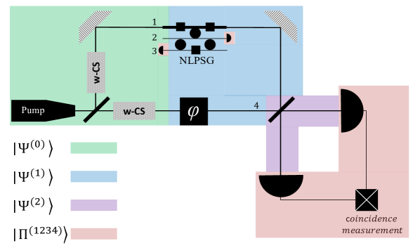
Figure 1: (Color online) The MRR NLPSG, with the ordinary three beam splitters used in the KLM implementation (see Fig.(4) in Appendix A) replaced by micro-ring resonators (MRRs) (black circles). The input state $|\Psi^{(0)}\rangle$ entering the upper and lower leg of the MZI are weak coherent states (w-CS) of the form $({\alpha}_{0}|0\rangle_{1}+{\alpha}_{1}|1\rangle_{1}+{\alpha}_{2}|2\rangle_{1})$ and $({\alpha}^{\prime}_{0}|0\rangle_{4}+{\alpha}^{\prime}_{1}|1\rangle_{4}+{\alpha}^{\prime}_{2}|2\rangle_{4})$, respectively, with the modes of the NLPSG in the upper leg of the MZI labeled (top-down) as $1,2,3$. Modes $2$ and $3$ are the ancilla modes to the NLPSG that are initially in the state $|1,0\rangle_{2,3}$. The lower leg, mode 4, of the MZI contains a PHASE shift element $e^{i\varphi a_{4}^{\dagger}a_{4}}$ which effectively sends ${\alpha}^{\prime}_{k}\to{\alpha}^{\prime}_{k}\,e^{i\,k\,\varphi}$. The action of $NLPSG_{123}\otimes PHASE_{4}$ produces the intermediate state $|\Psi^{(1)}\rangle$. The final element of the MZI is a BS of angle $\theta$ (such that $\theta=\pi/2$ is a 50:50 BS), whose output is $|\Psi^{(2)}\rangle$. Coincidence detection, producing the un-normalized state $|\tilde{\Psi}^{(2)}\rangle=\Pi^{1234}|\Psi^{(2)}\rangle$, is performed on the exiting modes 1 and 4, conditioned on the NLPSG ancilla modes $2$ and $3$, occurs with probability $\langle{\tilde{\Psi}^{(2)}}|{\tilde{\Psi}^{(2)}}\rangle$. The KLM NLPSG is obtained by replacing each black circle in the NLPSG sub-diagram by a single beam splitter with reflectivities $0\leq\eta_{i}\equiv r_{i}^{2}\leq 1$, where and $-1\leq r_{i}\leq 1$ are reflection coefficients for $i\in\{1,2,3\}$.

and a PHASE shift element in the other (lower) leg (mode $4$), as shown in Fig.(1). We will consider the case of finite detection efficiencies $\xi_{k}<1$ in each mode $1,2,3,4$, which can also can be considered as incorporating propagation and scattering losses. This will allow us to measure the success probability of the NLPSG in the presence of accidentals, namely, those coincidence counts that arise from states that are outside the isometry in Eq.(II). These accidentals add a noise floor to the the primary interference effect upon output from the MZI due to the mixing action of the BS and the use of detectors with finite detection efficiencies.

The initial state of the system entering the MZI is

$$|\Psi^{(0)}\rangle=({\alpha}_{0}|0\rangle_{1}+{\alpha}_{1}\,|1\rangle_{1}+{\alpha}_{2}|2\rangle_{1})\otimes|1,0\rangle_{2,3}\otimes({\alpha}^{\prime}_{0}|0\rangle_{4}+{\alpha}^{\prime}_{1}|1\rangle_{4}+{\alpha}^{\prime}_{2}|2\rangle_{4}),\quad\sum_{k=0}^{2}|{\alpha}_{k}|^{2}=\sum_{k=0}^{2}|{\alpha}^{\prime}_{k}|^{2}=1,$$ (3)

with modes $1,2,3$ associated with the NLPSG in the upper leg of the MZI and mode 4 in the lower leg (see labeling scheme in Fig.(1)). We can intuitively understand why this state will produce an interference pattern upon coincidence detection of modes 1 and 4 exiting the MZI. The lower leg of the MZI contains a PHASE shift element $e^{i\varphi a_{4}^{\dagger}a_{4}}$ which effectively sends ${\alpha}^{\prime}_{k}\to{\alpha}^{\prime}_{k}\,e^{i\,k\,\varphi}$. Recall that a lossless unitary BS preserves the total photon number entering its ports. Thus, as discussed in detail in Appendix B, a state $|n\rangle_{a}|m\rangle_{b}$ entering a BS will generate the $n+m+1$ states $\{|p\rangle_{a}|n+m-p\rangle_{b}\}$ where $p\in{0,1,\ldots,n+m}$ with (Wigner) rotation coefficients amplitudes. Thus, upon exit from the MZI, the input states $|0\rangle_{1}|2\rangle_{4}$ and $|2\rangle_{1}|0\rangle_{4}$ to the final BS will generate the output state $|1\rangle_{1}|1\rangle_{4}$ with phase factors proportional to $e^{i\,2\,\varphi}$ and $1$ respectively, and BS-dependent modified amplitudes. Similarly, the input state $|1\rangle_{1}|1\rangle_{4}$ to the final BS will also generate the output state $|1\rangle_{1}|1\rangle_{4}$ with phase factor $e^{i\,\varphi}$ and a BS-dependent modified amplitude. These two sets of terms, which we will consider individually, contribute to the primary coincidence interference pattern when we condition on the click/no click of the ancilla modes 2 and 3. Here a click detection means that, sans photon number resolving detectors, typical laboratory photon counting experiments are performed with bucket detectors (e.g. average efficiency APDs with $\xi_{k}\simeq 40\%$, or high efficiency SNSPDs with $\xi_{k}\simeq 85\%$) with the probability to detect $n$ photons scaling as $\xi^{n}$. Such higher order detections are called accidentals and contribute an additional noise floor (over that of detector dark counts, which we assume for simplicity to be zero) to the coincidence measurements.

In this work, we will keep track of such accidental terms using the reasonable approximation of detecting at most two photons in any single mode, $1,2,3,4$. We will see that upon output the set of input states $\{|0\rangle_{1}|2\rangle_{4},|2\rangle_{1}|0\rangle_{4}\}$ will generate the output state $|1,1,0,1\rangle_{1234}=|1,1\rangle_{14}|1,0\rangle_{23}$ upon which the primary interference will be observed, with the output ancilla modes remaining in their ideal “success heralding” state $|1,0\rangle_{23}$. The output state will also contain (orthogonal) 5-photon states with the the output ancilla modes not necessarily remaining in $|1,0\rangle_{23}$, plus various other photon Fock states in modes 1 and 4. Similarly, upon output, the input state $|1,1\rangle_{14}$ will also generate the ideal success state $|1,1,0,1\rangle_{1234}$, as well as 4-photon accidental states. A little forethought indicates that the amplitude of the output state $|1,1,0,1\rangle_{1234}$ will be of the form $({\alpha}_{0}\,{\alpha}^{\prime}_{2}\,A\,e^{i\,2\,\varphi}+{\alpha}_{2}\,{\alpha}^{\prime}_{0}\,B+{\alpha}_{1}\,{\alpha}^{\prime}_{1}\,Ce^{i\,\varphi})$ $\approx{\alpha}\,e^{i\,\varphi}\,(A(\theta)\,e^{i\,\varphi}+B(\theta)\,e^{-i\,\varphi}+C(\theta))$ leading to a primary success probability (squared amplitude) varying as $DC(\theta)+2\,A(\theta)\,B(\theta)\,\cos(2\,\varphi)+2\,C(\theta)\,\big{(}A(\theta)+B(\theta)\big{)}\cos(\varphi)$. Here $A(\theta),B(\theta),C(\theta)$ (taken real for simplicity) will depend on the final BS angle $\theta$, and $DC(\theta)=A(\theta)^{2}+B(\theta)^{2}+C(\theta)^{2}$ is the constant (independent of $\varphi$) contribution assuming unit detection efficiencies. When finite detection efficiencies are taken into account, there will be a prefactor scaling as $\xi^{6}\ll 1$ (assuming, for simplicity, equal detection efficiencies in all modes ) as well as both an “$AC(\theta,\phi)$” accidental term (dependent on the phase angle $\varphi$, arising from 4-photon output states generated from input states containing $|1\rangle_{1}$,  $|1\rangle_{4}$, or both) and a $DC(\theta)$ accidental term (arising from the 5-photon states generated by the $|0,2\rangle_{1,4}$ and $|2,0\rangle_{1,4}$ input states). Both these accidental states will contribute to the measured coincidence counts. However, these terms will be down in magnitude by factors of $\bar{n}\ll 1$ and $\bar{n}^{2}\lll 1$ respectively, from the primary interference probability. The details supporting this intuition will be worked out explicitly in the following sections.

III The NLPSG under arbitrary unitary evolution

Before we begin the main coincidence measurement calculation, let us first demonstrate the action of the unitary operator $U$ representing the NLPSG on modes 1, 2, 3. Under an arbitrary $N\times N$ unitary evolution $U$ on mode-$j$, the boson creation operators $a^{\dagger}_{in}$ are transformed linearly via Skaar et al. (2004)

$$a_{j,in}^{\dagger}\to U\,a_{j,in}^{\dagger}\,U^{\dagger}=\sum_{k=1}^{N}S^{T}_{jk}\,a_{k,out}^{\dagger}=\sum_{k=1}^{N}a_{k,out}^{\dagger}\,S_{kj},$$ (4)

where $T$ is transpose, defining the corresponding unitary matrix of coefficients $S_{kj}$ that act as transition coefficients for a photon initially in mode $j$ to be routed to output mode $k$. Henceforth, we will drop the $in,out$ subscript labels. The action of $U$ on the input state $|\psi_{(in)}\rangle_{123}=({\alpha}_{0}|0\rangle_{1}+{\alpha}_{1}\,|1\rangle_{1}+{\alpha}_{2}|2\rangle_{1})\otimes|1,0\rangle_{2,3}$ of Eq.(II) is then given by Scott et al. (2019)

$$|\psi_{(in)}\rangle_{123} = ({\alpha}_{0}|0\rangle_{1}+{\alpha}_{1}\,|1\rangle_{1}+{\alpha}_{2}|2\rangle_{1})\otimes|1,0\rangle_{2,3},$$

$$= \left({\alpha}_{0}+{\alpha}_{1}\,a_{1}^{\dagger}+{\alpha}_{2}\,\frac{a_{1}^{\dagger 2}}{\sqrt{2}}\,\right)\,a_{2}^{\dagger}\,|0,0,0\rangle_{123},$$

$$\xrightarrow{S}|\psi_{(out)}\rangle_{123} = \left[{\alpha}_{0}+{\alpha}_{1}\,\sum_{j=1}^{3}S_{j1}a^{\dagger}_{j}+{\alpha}_{2}\,\frac{1}{\sqrt{2}}\,\left(\sum_{j=1}^{3}S_{j1}a^{\dagger}_{j}\right)\,\left(\sum_{k=1}^{3}S_{k1}a^{\dagger}_{k}\right)\,\right]\,\left(\sum_{\ell=1}^{3}S_{\ell\,2}a^{\dagger}_{\ell}\right)\,|0,0,0\rangle_{123},\qquad$$ (5b)

$$\equiv |\psi^{NLPSG}_{(out)}\rangle_{123}+|\psi^{\perp}_{(out)}\rangle_{123},$$

where we have defined the 3-photon NLPSG state $|\psi^{NLPSG}_{(out)}\rangle_{123}$ as

$$|\psi^{NLPSG}_{(out)}\rangle_{123}\equiv\big{(}\beta_{0}\,{\alpha}_{0}\,|0\rangle_{1}+\beta_{1}\,{\alpha}_{1}\,|1\rangle_{1}-\beta_{2}\,{\alpha}_{2}\,|2\rangle_{1}\big{)}\otimes|1,0\rangle_{2,3}$$ (6)

with the $\beta_{k}$ coefficients defined as

$$\textrm{Condition-0:}\quad\beta_{0} = S_{22},$$ (7a)

$$\textrm{Condition-1:}\quad\beta_{1} = S_{11}\,S_{22}+S_{21}\,S_{12},$$ (7b)

$$\textrm{Condition-2:}\quad\beta_{2} = -S_{11}\,\left(S_{11}\,S_{22}+2\,S_{21}\,S_{12}\right),$$ (7c)

and

$$|\psi^{\perp}_{out}\rangle_{123}\equiv\left[{\alpha}_{0}\,\sum_{\ell\neq 2}S_{\ell\,2}a^{\dagger}_{\ell}+{\alpha}_{1}\,\sum_{j,\ell\neq\{(1,2),(2,1)\}}S_{j1}S_{\ell\,2}a^{\dagger}_{j}a^{\dagger}_{\ell}+\frac{1}{\sqrt{2}}\;{\alpha}_{2}\,\sum_{j,k,\ell\neq\{\textrm{perm}(1,1,2)\}}S_{j1}S_{k1}S_{\ell\,2}\,a^{\dagger}_{j}a^{\dagger}_{k}a^{\dagger}_{\ell}\right]\,|0,0,0\rangle_{123},$$ (8)

as the remaining “non-NLPSG” state orthogonal to $|\psi^{NLPSG}_{(out)}\rangle_{123}$. Successful operation of the NLPSG occurs when all three conditions Eq.(7a), Eq.(7b), and Eq.(7c) hold simultaneously, namely $\beta_{0}=\beta_{1}=\beta_{2}\equiv\beta$, in which case $|\psi^{NLPSG}_{(out)}\rangle_{123}\to\beta\,(a_{0}\,|0\rangle_{1}+a_{1}\,|1\rangle_{1}-{\alpha}_{2}\,|2\rangle_{1}$ with success probability $|\beta|^{2}$. The self consistency of all three conditions requires $S_{11}=1\mp\sqrt{2}$, with the physical solution ($|S_{11}|\leq 1$) demanding the solution with the minus sign. The remaining two conditions then demand that

$$P^{NLPSG}_{\textrm{success}}=|\beta|^{2}=|S_{22}|^{2}=\frac{1}{2}\,|S_{21}|^{2}\,|S_{12}|^{2},\qquad S_{11}=1-\sqrt{2}.$$ (9)

This is the operational scenario for the use of two NLPSG in the KLM-CNOT gate R. Okamoto and Takeuchi (2011); Scott et al. (2019); Alsing and Hach III (2018). At this stage, the unitary transformation $S$ is arbitrary. In the case of the KLM NLPSG implementation, $S$ is the product of three BS operators. For the MRR NLPSG implementation, as explored in Scott et al. (2019) and discussed in Appendix A, $S$ is the product of three MRR transfer matrix operators. Both these cases will be explored below, but for now we can remain unitarily agnostic, with a general $S$ matrix.

Finally, we note that if one’s sole purpose is simply to test the successful sign flip on the state $|2\rangle_{1}$, (say as an alternative to testing of the validity of the NLPSG with w-CS inputs) then this could also be accomplished by setting ${\alpha}_{1}\equiv 0$, using a co-linear SPDC (cl-SPDC) input state ${\alpha}_{0}\,|0\rangle_{1}+{\alpha}_{2}\,|2\rangle_{1}$ and lastly, only requiring that Condition-0 Eq.(7a), and Condition-2 Eq.(7c) hold, namely $\beta_{0}=\beta_{2}\equiv\beta$, with the value of $\beta_{1}$ unconstrained. While it is easier to generate w-CS than cl-SPDC states, the former which are also more operationally useful in optical quantum computing scenarios, it is informative to also explore the details of the latter case. It will turn out that both types of input states produce nearly identical coincidence interference patterns when the cl-SPDC input state scenario employ detectors operating at $40\%$ detection efficiencies, and the w-CS input state scenario employ detectors with $85\%$ detection efficiencies, both with NLPSG success probabilities of $|\beta|^{2}=1/4$. We will discuss the cl-SPDC scenario in Section V. For now we will explore the case of the general w-CS input state Eq.(5).

Before we begin the analysis of the MZI interferometer with a NLPSG in one leg and a PHASE shifter in the other, we first examine the POVM operator that is needed to project out the final state (from the MZI-transformed pure input state) that contributes to the coincidence counts.

IV click and no-click detection projection operators

Since the NLPSG is realized non-deterministically, we first review the concept of non-photon number resolving detection (bucket or click/no-click detection) that is typical of many laboratory experiments.

IV.1 Single mode detection

Consider a detector with probability (detection efficiency) $0\leq\xi\leq 1$ to detect one photon in a single mode $|1\rangle$, with the corresponding probability $1-\xi$ not to detect the single photon. Then the projection operators $\Pi_{NC}$ and $\Pi_{C}$ for a no-click and a click detection, respectively (i.e. non-photon number resolving detection) are given by

$$\Pi_{NC} = \sum_{n=0}^{\infty}\left(1-\xi\right)^{n}|n\rangle\langle n|\to|0\rangle\langle 0|\;\;\textrm{as}\;\;\xi\to 1,$$ (10a)

$$\Pi_{C} = I-\Pi_{NC}=\sum_{n=0}^{\infty}\left[1-\left(1-\xi\right)^{n}\right]|n\rangle\langle n|\to\sum_{n=1}^{\infty}|n\rangle\langle n|=I-|0\rangle\langle 0|\;\;\textrm{as}\;\;\xi\to 1,$$ (10b)

and hence the pair

$$\textrm{Single-mode detection POVM}=\{\Pi_{C},\Pi_{NC}\equiv I-P_{CC}\},$$ (11)

forms a dichotomous single mode detection POVM. Here, Eq.(10a) is intuitively understood as the probability $(1-\xi)^{n}$ not to detect the state $|n\rangle$ of $n$ photons, and for the no-click projector $\Pi_{NC}$ we then sum over all possible photon number states. In the limit of perfect (photon number resolving) detection $\xi\to 1$, we have that $\Pi_{NC}$ is just the projection onto the vacuum state $|0\rangle\langle 0|$. The opposite case of the detection one or more photons (a click) in the given mode is trivially given as $I-\Pi_{NC}$, with the intuitive $\xi\to 1$ limit of $I-|0\rangle\langle 0|=|1\rangle\langle 1|+|2\rangle\langle 2|+\cdots$ (i.e. the projector onto the state containing one or more photons).

The unnormalized state $|\tilde{\Psi}^{\prime}\rangle$ just after a click detection event is given by $|\tilde{\Psi}^{\prime}\rangle=\Pi_{C}\,|\Psi\rangle$ for the pure state $|\Psi\rangle$ just before the measurement. (Note: throughout the paper, we used a tilde to indicate an unnormalized state, whose norm yields a probability). The probability for the click measurement is then just the norm of this state $P_{C}=|||\tilde{\Psi}^{\prime}\rangle||^{2}=\langle\Psi|\Pi^{2}_{C}|\Psi\rangle$. (Note that while $\Pi_{C}$ is a measurement projection operator, it is not a von-Neumann projection operator in the sense that $\Pi^{2}_{C}\neq\Pi_{C}$. Along with $\Pi_{NC}$, it is an element of a POVM). This gives the expressions

$$P_{NC} = \textrm{Tr}[\Pi_{NC}\,|\Psi\rangle\langle\Psi|]=\sum_{n=0}^{\infty}\,q^{2}_{n}\,|\langle n|\Psi\rangle|^{2},\hskip 54.2025ptq_{n}=(1-\xi)^{n},\;\;q_{0}=1,\;q_{1}=1-\xi,$$ (12a)

$$P_{C} = \textrm{Tr}[\Pi_{C}\,|\Psi\rangle\langle\Psi|]=\sum_{n=0}^{\infty}\,p^{2}_{n}\,|\langle n|\Psi\rangle|^{2}=1-p_{NC},\;\;p_{n}=1-q_{n},\quad\;\;p_{0}=0,\;\;p_{1}=\xi.$$ (12b)

IV.2 Many mode detection

We can easily extend the concept of click and no-click detection to many modes. Consider first two modes $a$ and $b$. If one had perfect detection efficiency $\xi\to 1$, the situation in which we do not have a simultaneous coincidence click between modes $a$ and $b$ is given by

$$\Pi_{NCC}\hbox{ \raise-5.69054pt\hbox{$\textstyle{\rightarrow}\atop\scriptstyle{\xi\rightarrow 1}$} }|0\rangle_{a}\langle 0|\otimes I_{b}+I_{a}\otimes|0\rangle_{b}\langle 0|-|0\rangle_{a}\langle 0|\otimes|0\rangle_{b}\langle 0|,$$ (13)

where the first term is ”no-click” in detector $A$ and anything in detector $B$, the second term is the reverse situation, and the last term with the ”-” sign is needed to avoid the double counting of the vacuum projection $|0\rangle_{a}\langle 0|\otimes|0\rangle_{b}\langle 0|$ that occurs in the first two terms.

To extend Eq.(13) to imperfect detection $0\leq\xi_{a},\xi_{b}\leq 1$, we utilize Eq.(10b) to extend $I_{a}~{}-~{}|0\rangle_{a}\langle 0|\rightarrow\Pi^{(a)}_{C}=\sum_{n=0}^{\infty}\left[1-\left(1-\xi_{a}\right)^{n}\right]\,|n\rangle_{a}\langle n|\equiv\sum_{n=0}^{\infty}p^{(a)}_{n}|n\rangle_{a}\langle n|$ with $p^{(a)}_{n}=[1-\left(1-\xi_{a}\right)^{n}]$ the probability to detect a “click” of $n$ photons in mode-$a$ Fock state $|n\rangle_{a}$. Note that $p^{(a)}_{0}=0$ and $p^{(a)}_{1}=\xi_{a}$. Then, the probability to detect a click in both mode-$a$ and in mode-$b$, i.e. a coincidence count (CC), with finite detection efficiencies is just the product of the individual probabilities for mode-$a$ and mode-$b$, corresponding to the product of the projection operators for each mode, namely

$$\Pi^{(ab)}_{CC}=\Pi^{(a)}_{C}\otimes\Pi^{(b)}_{C} = \sum_{n=0}^{\infty}p^{(a)}_{n}|n\rangle_{a}\langle n|\otimes\sum_{m=0}^{\infty}p^{(b)}_{m}|m\rangle_{b}\langle m|,$$ (14a)

$$\equiv \sum_{n=0}^{\infty}\,\sum_{m=0}^{\infty}p^{(ab)}_{nm}|n,m\rangle_{ab}\langle n,m|,\quad p^{(ab)}_{nm}=[1-\left(1-\xi_{a}\right)^{n}]\,[1-\left(1-\xi_{b}\right)^{m}].\quad$$ (14b)

We see that the above expression has the correct limits, namely $p^{(ab)}_{00}=p^{(ab)}_{n0}=p^{(ab)}_{0m}=0$ appropriate for not detecting a coincidence click, and $p^{(ab)}_{11}=\eta_{a}\,\eta_{b}$. Lastly, the above expression reduces in the limit of unit detection efficiencies to $[I_{a}-|0\rangle_{a}\langle 0|]\otimes[I_{b}-|0\rangle_{b}\langle 0|]$ such that in the same limit the probability for no coincidence counts (NCC) $\Pi_{NCC}=I_{a}\otimes I_{b}-\Pi_{CC}$ reduces to the correct limiting form given by Eq.(13). Thus, the dichotomous two-element POVM defining two-mode coincidence click/no-click detection is given by

$$\textrm{Two-mode detection POVM}_{a,b}=\{\Pi^{(ab)}_{CC},\;\Pi^{(ab)}_{NCC}\equiv I_{a}\otimes I_{b}-\Pi^{(ab)}_{CC}\}.$$ (15)

This is easily generalized to arbitrary simultaneous coincidence clicks on $M$ modes $a_{i\in\{1,2,\ldots,M\}}$ via

$$\textrm{$M$-mode detection POVM}_{a_{1},\ldots,a_{M}} = \{\Pi^{({a_{1},\ldots,a_{M}})}_{CC},\;P^{({a_{1},\ldots,a_{M}})}_{NCC}\equiv I_{a_{1}}\otimes\ldots\otimes I_{a_{M}}-\Pi^{({a_{1},\ldots,a_{M}})}_{CC}\},\qquad$$ (16a)

$$\Pi^{(a_{1},\ldots,a_{M})}_{CC} = \bigotimes_{i=1}^{M}\Pi^{(a_{i})}_{C},\quad p^{(a_{1},\ldots,a_{M})}_{n_{1}\ldots\,n_{M}}=\prod_{i=1}^{M}p^{(a_{i})}_{n_{i}}=\prod_{i=1}^{M}[1-\left(1-\xi_{a_{i}}\right)^{n_{i}}].$$ (16b)

The takeaway point of this section is as follows. Under perfect detection efficiency, $\xi_{i}=1$ only the state $|1,1,0,1\rangle_{1234}$ will contribute to the probability interference pattern, as discussed in Section II. However, under finite, imperfect detection efficiencies, $\xi_{i}<1$, output states other than $|1,1,0,1\rangle_{1234}$ will also contribute to the output detected signal with varying probabilities. We will call such states accidentals, since they arise due to finite detection efficiencies. Note that in order to contribute to the total output signal, such states must contain at least one photon in each of modes 1, 2, and 4, and any number of photons in mode 3, i.e. $|n_{1},n_{2},n_{3},n_{4}\rangle_{1234}$ with $n_{1},n_{2},n_{4}\geq 1,\;n_{3}\geq 0$.

V Direct measurement of the NLPSG

In this section we analyze the MZI given in Fig.(1) containing the NLPSG in the upper leg of the MZI, with primary mode 1 and ancilla modes 2 and 3, and the PHASE shift element in the lower leg, mode 4. After the action of $NLPSG_{1,2,3}\otimes PHASE_{4}$, modes 1 and 4 interfere on a $BS_{14}$, and are subsequently coincidently detected upon exit from the MZI, while we simultaneously ask for a click detection on mode 2 and a no-click detection on mode 3. Our unitary operator is given by $\mathcal{U}=BS_{14}\cdot(NLPSG_{123}\otimes PHASE_{4})$ and our projection operator will be $\Pi^{(1,2,3,4)}\equiv\Pi^{(1)}_{C}\otimes\Pi^{(2)}_{C}\otimes\Pi^{(3)}_{NC}\otimes\Pi^{(4)}_{C}$. Note that we will explicitly implement (by hand) the phase shift element $PHASE_{4}=e^{i\,\varphi\,a^{\dagger}_{4}\,a_{4}}$ on mode 4, which simply has the net effect to transforming ${\alpha}^{\prime}_{k}\to{\alpha}^{\prime}_{k}\,e^{i\,k\,\varphi}$ on the w-CS₄ input state.

V.1 Preliminaries

As before, we allow the KLM triple BS (or triple MRR) operator on modes $1,2,3$ to be represented by $S_{ij}$, and the BS transformation on modes $1,4$ to be represented by $B_{ij}$. Extending these operators to $4\times 4$ matrix representations, we define

$$\mathcal{B}=\left[\begin{array}[]{cccc}\cos(\theta/2)&0&0&\sin(\theta/2)\\ 0&1&0&0\\ 0&0&1&0\\ -\sin(\theta/2)&0&0&\cos(\theta/2)\end{array}\right],\;\qquad\mathcal{S}=\left[\begin{array}[]{cccc}S_{11}&S_{12}&S_{13}&0\\ S_{21}&S_{22}&S_{23}&0\\ S_{31}&S_{32}&S_{32}&0\\ 0&0&0&1\end{array}\right],\qquad$$ (17)

where the rows and columns are labeled by the mode indices in the order $\{1,2,3,4\}$. (Note, the choice of the argument $\theta/2$ in the BS is so that a 50:50 BS is given by $\theta=\pi/2$). We define the product of these matrices as the unitary $\mathcal{U}$

$$\mathcal{U}\equiv\mathcal{B}\,\mathcal{S}=\left[\begin{array}[]{cccc}\cos(\theta/2)\,S_{11}&\cos(\theta/2)\,S_{12}&\cos(\theta/2)\,S_{13}&\sin(\theta/2)\\ S_{21}&S_{22}&S_{23}&0\\ S_{31}&S_{32}&S_{32}&0\\ -\sin(\theta/2)\,S_{11}&-\sin(\theta/2)\,S_{12}&-\sin(\theta/2)\,S_{13}&\cos(\theta/2)\end{array}\right].$$ (18)

The unitary transformation $\mathcal{U}$ affects the following transformations on the boson creation operators

$$a^{\dagger}_{i}\xrightarrow{S}\sum_{j=1}^{4}\,a^{\dagger}_{j}\,\mathcal{S}_{ji}\xrightarrow{BS}\sum_{j=1}^{4}\,\sum_{k=1}^{4}\,a^{\dagger}_{k}\,\mathcal{B}_{kj}\,\mathcal{S}_{ji}\equiv\sum_{k=1}^{4}\,a^{\dagger}_{k}\,\mathcal{U}_{ki},\quad\textrm{with}\;\;\mathcal{U}_{ki}=\sum_{j=1}^{4}\,\mathcal{B}_{kj}\,\mathcal{S}_{ji}.$$ (19)

This allows us to transform the initial state $|\Psi^{(0)}\rangle_{1234}\xrightarrow{\mathcal{U}}|\Psi^{(2)}\rangle_{1234}$ (see Fig.(1)). Upon coincidence detection of modes 1 and 4, with click/no-click detection on modes 2 and 3, we have the unnormalized post-measurement state $|\Psi^{(1)}\rangle_{1234}\xrightarrow{\Pi^{(1234)}}|\tilde{\Psi}^{(2)}\rangle_{1234}$ (indicated with a tilde) with detection probability $P_{1234}=|||\tilde{\Psi}^{(2)}\rangle_{1234}||^{2}$.

We begin by writing the initial state $|\Psi^{(0)}\rangle_{1234}$ , using $\sum_{i=0}^{2}|{\alpha}_{i}|^{2}=\sum_{i=0}^{2}|{\alpha}^{\prime}_{i}|^{2}=1$ as

$$|\Psi^{(0)}\rangle_{1234} = \big{[}{\alpha}_{0}|0\rangle_{1}+a_{1}|1\rangle_{1}+{\alpha}_{2}|2\rangle_{1}\big{]}\otimes|1,0\rangle_{2,3}\otimes\big{[}{\alpha}^{\prime}_{0}|0\rangle_{4}+{\alpha}^{\prime}_{1}|1\rangle_{4}+{\alpha}^{\prime}_{2}|2\rangle_{4}\big{]},$$ (20a)

$$= \left[{\alpha}_{0}\,{\alpha}^{\prime}_{0}\,a^{\dagger}_{2}+{\alpha}_{0}\,\dfrac{{\alpha}^{\prime}_{2}}{\sqrt{2}}\,a^{\dagger}_{2}\,\left(a^{\dagger}_{4}\right)^{2}+\dfrac{{\alpha}_{2}}{\sqrt{2}}\,{\alpha}^{\prime}_{0}\,\left(a^{\dagger}_{1}\right)^{2}\,a^{\dagger}_{2}\right.\left.+\;\dfrac{{\alpha}_{2}}{\sqrt{2}}\,\dfrac{{\alpha}^{\prime}_{2}}{\sqrt{2}}\,\left(a^{\dagger}_{1}\right)^{2}\,a^{\dagger}_{2}\,\left(a^{\dagger}_{4}\right)^{2}\right]\,|0,0,0,0\rangle_{1234}\qquad$$ (20c)

$$+ \left[{\alpha}_{0}\,{\alpha}^{\prime}_{1}\,a^{\dagger}_{2}\,a^{\dagger}_{4}+{\alpha}_{1}\,{\alpha}^{\prime}_{0}\,a^{\dagger}_{1}\,a^{\dagger}_{2}+{\alpha}_{1}\,{\alpha}^{\prime}_{1}\,a^{\dagger}_{1}\,a^{\dagger}_{2}\,a^{\dagger}_{4}+{\alpha}_{1}\,\dfrac{{\alpha}^{\prime}_{2}}{\sqrt{2}}\,a^{\dagger}_{1}\,a^{\dagger}_{2}\,(a^{\dagger}_{4})^{2}\right.$$

$$\left.\hskip 198.7425pt+\,\dfrac{{\alpha}_{2}}{\sqrt{2}}\,{\alpha}^{\prime}_{1}\,(a^{\dagger}_{1})^{2}\,a^{\dagger}_{2}\,a^{\dagger}_{4}\right]\,|0,0,0,0\rangle_{1234},$$

$$\equiv |\Psi_{02^{\prime};2^{\prime}0}^{(0)}\rangle+|\Psi_{1,1^{\prime}}^{(0)}\rangle,$$ (20d)

where the input state $|\Psi^{(0)}\rangle_{1234}$ has been separated into two branches. Eq.(20c) separates out that branch $|\Psi_{02^{\prime};2^{\prime}0}^{(0)}\rangle$ of the input state that contains only the states $|0\rangle_{k}$ and $|2\rangle_{k}$ in modes $k=1,4$. Eq.(20c) $|\Psi_{1,1^{\prime}}^{(0)}\rangle$ separates out the remaining branch of the input state $|\Psi^{(0)}\rangle_{1234}$ that involve either input states $|1\rangle_{1}$ , $|1\rangle_{4}$, or both.

In the following, we will first concentrate on transformation of the input state $|\Psi_{02^{\prime};2^{\prime}0}^{(0)}\rangle$ which after the measurement involves the single $3$-photon output state $|1,1,0,1\rangle_{1234}$, and only 5-photon accidental states. Subsequently, we will analyze the transformation of the remaining input state $|\Psi_{1,1^{\prime}}^{(0)}\rangle$, which after the measurement also involves the output state $|1,1,0,1\rangle_{1234}$, but now with only 4-photon accidental states.

V.2 Transformation of the input state $|\Psi_{02^{\prime};2^{\prime}0}^{(0)}\rangle_{1234}$

After applying the $4\times 4$ unitary $\mathcal{U}=BS_{14}\cdot(NLPSG_{123}\otimes PHASE_{4})$ on the mode operators, as illustrated in Fig.(1), we have (note: under $PHASE_{4}$ we have $|n\rangle_{4}\to e^{i\,n\,\varphi}\,|n\rangle_{4}$ for $n\in\{0,1,2\}$).

$$|\Psi^{(0)}_{0,2^{\prime};2,0^{\prime}}\rangle_{1234} \xrightarrow{\textrm{\tiny NLPSG}_{123}\otimes\textrm{\tiny PHASE}_{4}} |\Psi^{(1)}_{0,2^{\prime};2,0^{\prime}}\rangle_{1234}\xrightarrow{BS_{14}}|\Psi^{(2)}_{0,2^{\prime};2,0^{\prime}}\rangle_{1234},$$ (21a)

$$= \left[{\alpha}_{0}\,{\alpha}^{\prime}_{0}\,\sum_{j=1}^{4}\,a^{\dagger}_{j}\,\mathcal{U}_{j2}+{\alpha}_{0}\,\dfrac{{\alpha}^{\prime}_{2}}{\sqrt{2}}\,e^{i\,2\,\varphi}\,\left(\sum_{j=1}^{4}\,a^{\dagger}_{j}\,\mathcal{U}_{j2}\right)\,\left(\cos(\theta/2)a^{\dagger}_{4}+\sin(\theta/2)\,a^{\dagger}_{1}\right)^{2}\right.$$

$$+ \dfrac{{\alpha}_{2}}{\sqrt{2}}\,\,{\alpha}^{\prime}_{0}\,\left(\sum_{j=1}^{4}\,a^{\dagger}_{j}\,\mathcal{U}_{j1}\right)\left(\sum_{k=1}^{4}\,a^{\dagger}_{k}\,\mathcal{U}_{k1}\right)\left(\sum_{\ell=1}^{4}\,a^{\dagger}_{\ell}\,\mathcal{U}_{\ell 2}\right)$$

$$+ \left.\frac{{\alpha}_{2}}{\sqrt{2}}\,\frac{{\alpha}^{\prime}_{2}}{\sqrt{2}}\,e^{i\,2\,\varphi}\,\left(\sum_{j=1}^{4}\,a^{\dagger}_{j}\,\mathcal{U}_{j1}\right)\left(\sum_{k=1}^{4}\,a^{\dagger}_{k}\,\mathcal{U}_{k1}\right)\left(\sum_{\ell=1}^{4}\,a^{\dagger}_{\ell}\,\mathcal{U}_{\ell 2}\right)\,\left(\cos(\theta/2)a^{\dagger}_{4}+\sin(\theta/2)\,a^{\dagger}_{1}\right)^{2}\right],\qquad\;$$

$$\xrightarrow{\Pi^{(1234)}} |T_{0,2^{\prime}}\rangle_{1234}+|T_{2,0^{\prime}}\rangle_{1234}+|T_{2,2^{\prime}}\rangle_{1234}.$$ (21b)

where in Eq.(21a) we have explicitly carried out the BS transformation on mode-$4$, $a^{\dagger}_{4}\rightarrow\cos(\theta/2)\,a^{\dagger}_{4}+\sin(\theta/2)\,a^{\dagger}_{1}$, (but not on mode-$1$). Additionally, we have explicitly implemented the the PHASE gate $I_{123}\otimes\,e^{i\,a^{\dagger}_{4}\,a_{4}\,\varphi}$ on mode-$4$, which on states sends $|0\rangle_{4}\rightarrow|0\rangle_{4}$ and $|2\rangle_{4}\rightarrow e^{i\,2\,\varphi}\,|2\rangle_{4}$, and which we have incorporated by hand, having the net effect of sending ${\alpha}^{\prime}_{2}\rightarrow{\alpha}^{\prime}_{2}\,e^{i\,2\,\varphi}$. Here the states $|T_{i,j^{\prime}}\rangle_{1234}$ listed in Eq.(21b), arising from the transformation of the input state $|i\rangle_{1}\,|j\rangle_{4}$, are those three or more photon states that survive under measurement projection. Recall that $p^{(k)}_{0}=0$ for for mode $k$, so that the states that remain after projection must contain three or more photons, with at least one photon in each of modes $k=\{1,2,4\}$.

The individual states are given by

$$|T_{0,2^{\prime}}\rangle_{1234} = {\alpha}_{0}\,\dfrac{{\alpha}^{\prime}_{2}}{\sqrt{2}}\,e^{i\,2\,\varphi}\,\sin(\theta)\,\mathcal{U}_{22}|1,1,0,1\rangle_{1234},$$ (22)

$$= {\alpha}_{0}\,\dfrac{{\alpha}^{\prime}_{2}}{\sqrt{2}}\,e^{i\,2\,\varphi}\,\sin(\theta)\,S_{22}|1,1,0,1\rangle_{1234},$$

and

$$|T_{2,0^{\prime}}\rangle_{1234} = \frac{{\alpha}_{2}}{\sqrt{2}}\,{\alpha}^{\prime}_{0}\,\left[\mathcal{U}_{11}\,\mathcal{U}_{21}\,\mathcal{U}_{42}+\mathcal{U}_{11}\,\mathcal{U}_{41}\,\mathcal{U}_{22}+\mathcal{U}_{21}\,\mathcal{U}_{11}\,\mathcal{U}_{42}+\mathcal{U}_{21}\,\mathcal{U}_{41}\,\mathcal{U}_{12}+\mathcal{U}_{41}\,\mathcal{U}_{11}\,\mathcal{U}_{22}+\mathcal{U}_{41}\,\mathcal{U}_{21}\,\mathcal{U}_{12}\right]\,|1,1,0,1\rangle_{1234},\qquad\;\;$$ (23)

$$= \frac{{\alpha}_{2}}{\sqrt{2}}\,{\alpha}^{\prime}_{0}\,\sin(\theta)\left[-S_{11}\,\left(S_{11}\,S_{22}+S_{21}\,S_{12}\right)\right]\,|1,1,01\rangle_{1234},$$

where we recognize $\beta_{0}$ from Eq.(7a) as the amplitude in Eq.(22), and $\beta_{2}$ from Eq.(7c) as the amplitude in Eq.(23). Thus, combining the above two results and upon imposing Condition-0 Eq.(7a) and Condition-2 Eq.(7c) only, which ensures that $\beta_{0}=\beta_{2}\equiv\beta$, we already have our primary interference contribution, namely

$$|T_{0,2^{\prime}}\rangle_{1234}+|T_{2,0^{\prime}}\rangle_{1234} = \frac{1}{\sqrt{2}}\,\sin(\theta)\,\left[-S_{11}\,\left(S_{11}\,S_{22}+S_{21}\,S_{12}\right)\,{\alpha}^{\prime}_{0}\,{\alpha}_{2}+{\alpha}_{0}\,{\alpha}^{\prime}_{2}\,e^{i\,2\,\varphi}\,S_{22}\right]\,|1,1,0,1\rangle_{1234},$$ (24)

$$= \frac{1}{\sqrt{2}}\,\sin(\theta)\,\beta\,\left[{\alpha}^{\prime}_{0}\,{\alpha}_{2}+{\alpha}_{0}\,{\alpha}^{\prime}_{2}\,e^{i\,2\,\varphi}\right]\,|1,1,0,1\rangle_{1234},\;\;\textrm{{if} impose Conditions 0 \& 2},\qquad\;\;$$ (25)

$$\rightarrow \sqrt{2}\,\sin(\theta)\,\beta\,|{\alpha}_{0}|\,|{\alpha}_{2}|\,e^{i\,\varphi}\,\cos(\varphi)\,|1,1,0,1\rangle_{1234},\quad\textrm{for}\;{\alpha}^{\prime}_{0}={\alpha}_{0}\;\textrm{\&}\;{\alpha}^{\prime}_{2}={\alpha}_{2}.$$ (26)

This last term leads to a coincidence probability arising only from the $3$-photon state $|1,1,0,1\rangle_{1234}$ contribution:

$$P^{(3-\textrm{photons})}_{1234}\rightarrow 2\,\xi_{1}^{2}\,\xi_{2}^{2}\,\xi_{4}^{2}\,\sin^{2}(\theta)\,|\beta|^{2}\,|{\alpha}_{0}|^{2}\,|{\alpha}_{2}|^{2}\,\cos^{2}(\varphi),$$ (27)

where we have also included the finite detection efficiency factors.

Lastly, the remaining 5-photon states $|T_{2,2^{\prime}}\rangle_{1234}$ generated from $\mathcal{U}$ acting on $|\Psi^{(0)}_{0,2^{\prime};2,0^{\prime}}\rangle$, which do not contribute to the above primary interference pattern are given by

$$|T_{2,2^{\prime}}\rangle_{1234} = {\alpha}_{2}\,{\alpha}^{\prime}_{2}\,e^{i\,2\,\varphi}\,\Big{(}$$ (28)

$$|1,2,0,2\rangle_{1234}\,\left[\sin(\theta)\,\mathcal{U}^{(cs)}_{202}+\sin^{2}(\theta/2)\,\mathcal{U}^{(ss)}_{202}\right]$$

$$+ |1,2,1,1\rangle_{1234}\,\left[\sin(\theta)\,\mathcal{U}^{(cs)}_{211}\right]$$

$$+ |1,1,1,2\rangle_{1234}\,\left[\sin(\theta)\,\mathcal{U}^{(cs)}_{112}+\sin^{2}(\theta/2)\,\mathcal{U}^{(ss)}_{112}\right]$$

$$+ |1,1,2,1\rangle_{1234}\,\left[\sin(\theta)\,\mathcal{U}^{(cs)}_{121}\right]$$

$$+ |2,2,0,1\rangle_{1234}\,\left[\cos^{2}(\theta/2)\,\mathcal{U}^{(cc)}_{201}+\sin(\theta)\,\mathcal{U}^{(cs)}_{201}\right]$$

$$+ |2,1,1,1\rangle_{1234}\,\left[\cos^{2}(\theta/2)\,\mathcal{U}^{(cc)}_{111}+\sin(\theta)\,\mathcal{U}^{(cs)}_{111}\right]$$

$$+ \left.|2,1,0,2\rangle_{1234}\,\left[\cos^{2}(\theta/2)\,\mathcal{U}^{(cc)}_{102}+\sin(\theta)\,\mathcal{U}^{(cs)}_{102}+\sin^{2}(\theta/2)\,\mathcal{U}^{(ss)}_{102}\right]\right),$$

where the various matrix elements $\{\mathcal{U}^{(cs)}_{202},\mathcal{U}^{(ss)}_{202},\ldots\}$ in terms of $\mathcal{U}_{ij}$ are listed explicitly in the Appendix Appendix C. (Note: $\{cc,cs,ss,\}$ superscripts indicate that terms are multiplied by $\{\cos^{2}(\theta/2),2\,\cos(\theta/2)\sin(\theta/2),\sin^{2}(\theta/2)\}$ and $\{c,s\}$ superscripts indicate terms are multiplied by $\{\cos(\theta/2),\,\sin(\theta/2)\}$. The subscripts $i,j,k$ indicate that the amplitudes multiply the state $|i,j,k\rangle_{2,3,4}$). The important point to note is that by containing 5-photon terms $|T_{2,2^{\prime}}\rangle_{1234}$ is automatically orthogonal to the 3-photon state $|1,1,0,1\rangle_{1234}$ upon which the primary interference effects occurs. Additionally, each term in Eq.(28) is multiplied by $e^{i\,2\,\varphi}$, and is also orthogonal to every other term in $|T_{2,2^{\prime}}\rangle_{1234}$. Hence, upon squaring these amplitudes for the probability, these terms simply contribute to a (BS-angle dependent) dc accidental term $DC(\theta)$, independent of the phase angle $\varphi$.

V.3 Transformation of the input state $|\Psi_{1;1^{\prime}}^{(0)}\rangle_{1234}$

Turning to the the transformation of the terms listed in Eq.(20c) containing $|1\rangle_{1}$, $|1\rangle_{4}$ or both, we have

$$|\Psi^{(0)}_{1,1^{\prime}}\rangle_{1234} \xrightarrow{\textrm{\tiny NLPSG}_{123}\otimes\textrm{\tiny PHASE}_{4}} |\Psi^{(1)}_{1,1^{\prime}}\rangle_{1234}\xrightarrow{BS_{14}}|\Psi^{(2)}_{1,1^{\prime}}\rangle_{1234},$$ (29c)

$$= \left[{\alpha}_{0}\,{\alpha}^{\prime}_{1}\,\left(\sum_{j=1}^{4}a^{\dagger}_{j}\,\mathcal{U}_{j1}\right)\,\left(\cos(\theta/2)\,a^{\dagger}_{4}+\sin(\theta/2)\,a^{\dagger}_{1}\right)+{\alpha}_{1}\,{\alpha}^{\prime}_{0}\,\left(\sum_{j=1}^{4}a^{\dagger}_{j}\,\mathcal{U}_{j1}\right)\,\left(\sum_{k=1}^{4}a^{\dagger}_{k}\,\mathcal{U}_{k2}\right)\,\right.$$

$$+\,{\alpha}_{1}\,{\alpha}^{\prime}_{1}\,e^{i\,\varphi}\,\left(\sum_{j=1}^{4}a^{\dagger}_{j}\,\mathcal{U}_{j1}\right)\,\left(\sum_{k=1}^{4}a^{\dagger}_{k}\,\mathcal{U}_{k2}\right)\,\left(\cos(\theta/2)\,a^{\dagger}_{4}+\sin(\theta/2)\,a^{\dagger}_{1}\right)$$

$$+\,{\alpha}_{1}\,\dfrac{{\alpha}^{\prime}_{2}}{\sqrt{2}}\,e^{i\,2\,\varphi}\,\left(\sum_{j=1}^{4}a^{\dagger}_{j}\mathcal{U}_{j1}\right)\,\left(\sum_{k=1}^{4}a^{\dagger}_{k}\mathcal{U}_{k2}\right)\,\left(\cos(\theta/2)\,a^{\dagger}_{4}+\sin(\theta/2)\,a^{\dagger}_{1}\right)^{2}$$

$$\left.+\,\dfrac{{\alpha}_{2}}{\sqrt{2}}\,{\alpha}^{\prime}_{1}\,e^{i\,\varphi}\,\left(\sum_{j=1}^{4}a^{\dagger}_{j}\mathcal{U}_{j1}\right)\,\left(\sum_{k=1}^{4}a^{\dagger}_{k}\mathcal{U}_{k1}\right)\,\left(\sum_{\ell=1}^{4}a^{\dagger}_{\ell}\mathcal{U}_{\ell 2}\right)\,\left(\cos(\theta/2)\,a^{\dagger}_{4}+\sin(\theta/2)\,a^{\dagger}_{1}\right)\right]\,|0,0,0,0\rangle_{1234},\qquad\;$$

$$\xrightarrow{\Pi^{(1234)}}|T_{1,1^{\prime}}\rangle_{1234}+|T_{1,2^{\prime}}\rangle_{1234}+|T_{2,1^{\prime}}\rangle_{1234}.$$

Following the same procedure as above, the state that survives after measurement projection and contributes to the primary coincidence interference effect is

$$|T_{1,1^{\prime}}\rangle_{1234} = {\alpha}_{1}\,{\alpha}^{\prime}_{1}\,e^{i\,\varphi}\,|1,1,0,1\rangle_{1234}\,\left[\cos(\theta/2)\,\mathcal{U}^{\prime(c)}_{101}+\sin(\theta/2)\,\mathcal{U}^{\prime(s)}_{101}\,\right],$$ (30)

$$= {\alpha}_{1}\,{\alpha}^{\prime}_{1}\,e^{i\,\varphi}\,|1,1,0,1\rangle_{1234}\;\beta_{1}\cos(\theta),$$

which arises from the transformation of the input state $|1\rangle_{1}\,|1\rangle_{4}$. In the above we have defined

$$\beta_{1}\equiv S_{11}\,S_{22}+S_{21}\,S_{12}\hbox{ \raise-5.69054pt\hbox{$\textstyle{\longrightarrow}\atop\scriptstyle{\beta\to\beta_{max}=1/2}$} }\,\beta_{max}=1/2,\quad(\beta_{max}^{2}=1/4),$$ (31)

where $\beta_{1}\to\beta=1/2$ if we were to impose Condition-1, Eq.(7b) in addition to the previously imposed Condition-0, Eq.(7a) and Condition-2, Eq.(7c), which would then make $\beta^{2}\to\beta^{2}_{max}=1/4$.

The remaining 4-photon orthogonal accidental states arising from the transformation of the input states $|1\rangle_{1}\,|2\rangle_{4}$ and $|2\rangle_{1}\,|1\rangle_{4}$ are given by

$$|T_{1,2^{\prime}}\rangle_{1234} + |T_{2,1^{\prime}}\rangle_{1234}=$$ (32)

$$\Big{(}e^{i\,\varphi}\,|1,2,0,1\rangle_{1234}\,\left[{\alpha}_{1}\,{\alpha}^{\prime}_{2}\,e^{i\,\varphi}\,\sin(\theta)\,\mathcal{U}^{\prime(cs)}_{201}+{\alpha}_{2}\,{\alpha}^{\prime}_{1}\,\left(\cos(\theta/2)\,\mathcal{U}^{\prime(c)}_{201}+\sin(\theta/2)\,\mathcal{U}^{\prime(s)}_{201}\right)\right]$$

$$+\,e^{i\,\varphi}\,|1,1,1,1\rangle_{1234}\,\left[{\alpha}_{1}\,{\alpha}^{\prime}_{2}\,e^{i\,\varphi}\,\sin(\theta)\,\mathcal{U}^{\prime(cs)}_{111}+{\alpha}_{2}\,{\alpha}^{\prime}_{1}\,\left(\cos(\theta/2)\,\mathcal{U}^{\prime(c)}_{111}+\sin(\theta/2)\,\mathcal{U}^{\prime(s)}_{111}\right)\right]$$

$$+\,e^{i\,\varphi}\,|1,1,0,2\rangle_{1234}\,\left[{\alpha}_{1}\,{\alpha}^{\prime}_{2}\,e^{i\,\varphi}\,\left(\sin(\theta)\,\mathcal{U}^{\prime(cs)}_{102}+\cos^{2}(\theta/2)\,\mathcal{U}^{\prime(cc)}_{102}\right)+{\alpha}_{2}\,{\alpha}^{\prime}_{1}\,\left(\cos(\theta/2)\,\mathcal{U}^{\prime(c)}_{102}+\sin(\theta/2)\,\mathcal{U}^{\prime(s)}_{102}\right)\right]$$

$$+\,e^{i\,\varphi}\,|2,1,0,1\rangle_{1234}\,\left[{\alpha}_{1}\,{\alpha}^{\prime}_{2}\,e^{i\,\varphi}\,\left(\sin(\theta)\,\mathcal{U}^{\prime(cs)}_{101}+\sin^{2}(\theta/2)\,\mathcal{U}^{\prime(ss)}_{101}\right)+{\alpha}_{2}\,{\alpha}^{\prime}_{1}\,\left(\cos(\theta/2)\,\mathcal{U}^{\prime(c)}_{101}+\sin(\theta/2)\,\mathcal{U}^{\prime(s)}_{101}\right)\right]\Big{)},\qquad\;\;$$

Again, the various matrix elements $\{\mathcal{U}^{\prime(cs)}_{202},\mathcal{U}^{\prime(ss)}_{202},\ldots\}$ in terms of $\mathcal{U}_{ij}$ are listed explicitly in Appendix C. Note that squaring each of the above amplitudes will generate a $\cos(\varphi)$ higher-order interferences in the accidentals.

V.4 Form of the unnormalized post measurement state

The complete output state upon transformation by $\mathcal{U}$ for a general w-CS input states on mode 1 and 4 is then

$$|\Psi^{(0)}\rangle_{1234}\xrightarrow{\mathcal{U}}|\Psi^{(2)}\rangle_{1234} \equiv |T_{0,2^{\prime}}\rangle_{1234}+|T_{2,0^{\prime}}\rangle_{1234}+|T_{2,2^{\prime}}\rangle_{1234},$$ (33)

$$+ |T_{1,1^{\prime}}\rangle_{1234}+|T_{1,2^{\prime}}\rangle_{1234}+|T_{2,1^{\prime}}\rangle_{1234}.$$

where the top line comes from the transformation of $|\Psi_{02^{\prime};20}^{(0)}\rangle$ and the bottom line arises from the transformation of $|\Psi_{1,1^{\prime}}^{(0)}\rangle$. Recall that the state after projection is given by

$$|\tilde{\Psi}^{(2)}\rangle_{1234} \equiv \Pi^{1234}\,|\Psi^{(2)}\rangle_{1234}=\sum_{n,m,r,s=0}^{4\;\prime}\,p^{(1)}_{n}\,p^{(2)}_{m}\,\left(1-p^{(3)}_{r}\right)\,p^{(4)}_{s}\,|n,m,r,s\rangle_{1234}\langle{n,m,r,s}|{\Psi^{(2)}}\rangle_{1234},\qquad$$ (34)

where the prime on the summation indicates that we are in the approximation that each mode contains at most two photons. Since $p^{(k)}_{0}=0$, only states with at least one photon in modes $k\in\{1,2,4\}$ survive the measurement projection, and therefore $|\tilde{\Psi}^{(2)}\rangle_{1234}$ contains the 3-photon state $|1,1,0,1\rangle_{1234}$, plus 4- and 5-photon accidental states that also contribute to the coincidence counts when detectors with finite detection efficiencies are employed.

The primary coincidence interference term arises from the $|1,1,0,1\rangle_{1234}$ portion of $|\tilde{\Psi}^{(2)}\rangle_{1234}$ which has the form

$$|\tilde{\Psi}^{(2)}\rangle=(\textrm{prefactor})^{1/2}\times\,\left[\beta\,f_{3}(\theta,\varphi)\,|1,1,0,1\rangle_{1234}+\alpha\,|\tilde{\Psi}_{4}^{(2)}(\theta,\varphi)\rangle_{1234}+\alpha^{2}\,|\tilde{\Psi}_{5}^{(2)}(\theta)\rangle_{1234}\right],$$ (35)

where we have defined the prefactor as

$$(\textrm{prefactor})^{1/2}=\dfrac{\xi_{1}\,\xi_{2}\,\xi_{4}\,\alpha^{2}\,e^{i\varphi}}{1+\alpha^{2}+\alpha^{4}/2}=\dfrac{\xi_{1}\,\xi_{2}\,\xi_{4}\,\bar{n}\,e^{i\varphi}}{1+\bar{n}+\bar{n}^{2}/2},$$ (36)

where $\bar{n}\approx\alpha^{2}$ is the mean number of photons in the w-CS. Additionally, we define the interference amplitude $f_{3}(\theta,\varphi)$, after factoring out $\beta$, as

Interference Amplitude: (38)

$$\textrm{(i)}\;f_{3}(\theta,\varphi)=\sin(\theta)\,\cos(\varphi)+(\beta_{1}/\beta)\,\cos(\theta),\textrm{ {only assuming} Condition-$0$ \& Condition-$2$, i.e\;\;}\beta_{0}=\beta_{2}\equiv\beta,\qquad$$

$$\textrm{(ii)}\;f_{3}(\theta,\varphi)\to\sin(\theta)\,\cos(\varphi)+\cos(\theta),\;\hskip 28.90755pt\textit{additionally}\textrm{ imposing Condition-$1$, i.e.\;}\beta_{0}=\beta_{1}=\beta_{2}\equiv\beta.$$

Here $|\tilde{\Psi}_{4}^{(2)}(\theta,\varphi)\rangle_{1234}$ and $|\tilde{\Psi}_{5}^{(2)}(\theta)\rangle_{1234}$ are (unnormalized state) contributions from the $4$-photon and $5$-photon states respectively, that contribute to the accidentals, and we have used ${\alpha}^{\prime}_{k}={\alpha}_{k}=\dfrac{\alpha^{k}}{\sqrt{1+\alpha^{2}+\alpha^{4}/2}}$ in Eq.(36) for simplicity. $\theta$ is the BS angle (with $\theta=\pi/2$ for a 50:50 BS), and $\varphi$ is the phase shift angle in mode-$4$. The final interference probability $P_{1234}$, imposing all three Conditions-0,1,2 then has the form

$$P_{1234} = ||\,|\tilde{\Psi}^{(2)}\rangle_{1234}||^{2}=\left[\dfrac{\xi^{2}_{1}\,\xi^{2}_{2}\,\xi^{2}_{4}\,\bar{n}^{2}}{(1+\bar{n}+\bar{n}^{2}/2)^{2}}\right]\,\Big{[}\beta^{2}\,f^{2}_{3}(\theta,\varphi)+\bar{n}\,AC(\theta,\varphi)+\bar{n}^{2}\,DC(\theta)\Big{]},$$ (39b)

$$\bar{n}=\alpha^{2},\quad AC(\theta,\varphi)={}_{1234}\langle{\tilde{\Psi}_{4}^{(2)}}|{\tilde{\Psi}_{4}^{(2)}}\rangle_{1234}\quad DC(\theta)={}_{1234}\langle{\tilde{\Psi}_{5}^{(2)}}|{\tilde{\Psi}_{5}^{(2)}}\rangle_{1234}.$$

Note that the first and third terms in the right square brackets of Eq.(39b) arise from input states on mode-$1$ and $4$ that contain only 0 and 2 photons when a 50:50 BS ($\theta=\pi/2$) is used (i.e. $\cos(\theta)\to 0$ wipes out the interference contributions arising from the addition of the $|1\rangle_{1}$ and $|1\rangle_{4}$ input states). This is of course, just the well known HOM BS-induced interference effect in the context of our NLPSG MZI C.K. Hong and Mandel (1987); Hach III et al. (2014). Also note that the first (interference) term in Eq.(39b) is of $\mathcal{O}(\beta^{2})\sim\mathcal{O}(1)$, while each additional (accidentals) term scales as $\mathcal{O}(\bar{n})\ll 1$ and $\mathcal{O}(\bar{n}^{2})\lll 1$, respectively. Eq.(39b) with Eq.(39b) is one of the main results of this work, to which we will now specialize to both the KLM and MRR implementation of the NLPSG.

In Fig.(2) we plot the scaled probability $P^{\prime(\theta=\pi/2,\varphi)}_{1234}$ (i.e. defined from Eq.(39b) as $P_{1234}~{}\equiv~{}\textrm{prefactor}\times P^{\prime}_{1234}$ ) for coincidences (left) KLM, (right) MRR using co-linear SPDC (cl-SPDC, dashed) and weak coherent (w-CS, solid) input states with a 50:50 BS ($\theta=\pi/2$), and $|{\alpha}_{2}/{\alpha}_{0}|^{2}=0.1$ with finite detection efficiencies (gray, black) $\xi_{1}=\xi_{2}=\xi_{4}\equiv\xi=\{0.40,0.85\}$, at the optimal reflection coefficients $r^{*2}_{1}=r^{*2}_{3},\,r^{*2}_{2}\Rightarrow|\beta|^{2}=1/4$.

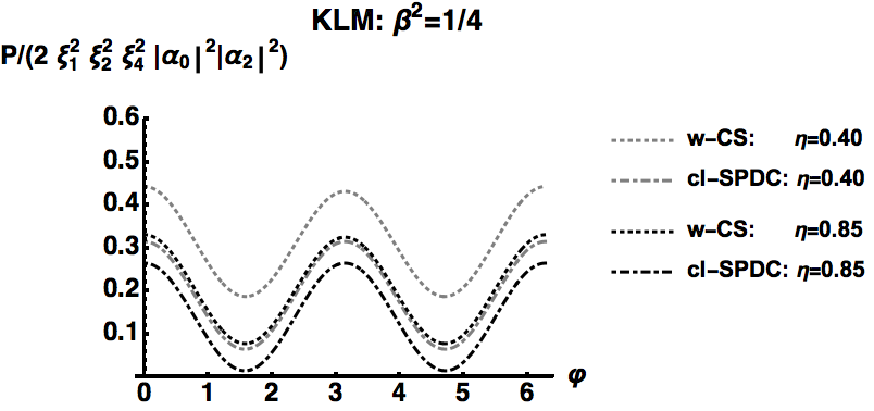
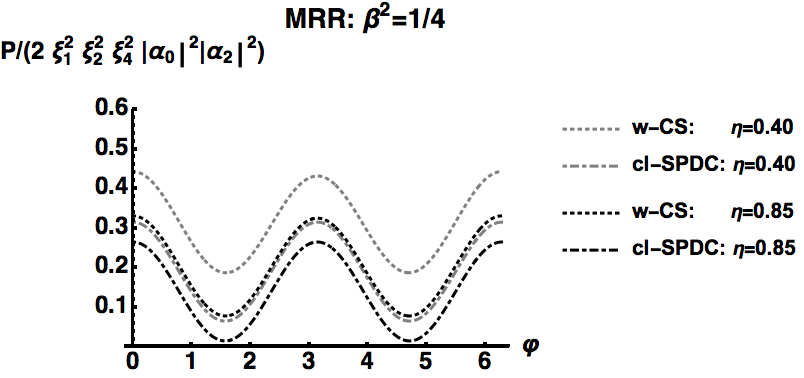
Figure 2: Plot of $P^{\prime}_{1234}$ from Eq.(39b) for the (left) KLM, (right) MRR NLPSG for $\beta^{2}=1/4$ for (dotted) w-CS input states and (dot-dashed) cl-SPDC input states with detection efficiencies (gray) $40\%$ and (black) $85\%$. The left and right graphs are identical.

The (left) KLM and (right) MRR curves are identical. The reason these curves are identical, is that even though $S^{(MRR)}$ and $S^{(KLM)}$ are not strictly identical, i.e. $S^{(MRR)}\neq S^{(KLM)}$, they are effectively identical in the sense that the upper left $2\times 2$ sub-matrix $\small{\left(\begin{array}[]{cc}S_{11}&S_{21}\\ S_{21}&S_{22}\end{array}\right)}$, of each unitary matrix are identical at $\beta^{2}=1/4$, which now enforces Condition-1, along with Condition-0 and Condition-2 which were previously satisfied, while the third row and third column of the each unitary matrix are different. This is how the MRR-NLPSG encompasses the KLM-NLPSG (since the former solution was modeled after the latter’s). This is not the case at other values of $\beta^{2}\neq 1/4$.

The new feature using the MRR-NLPSG is the one-dimensional manifold relationship between the phyisical transmission coefficients $\tau_{i}$ and $\eta_{i}=\eta_{i}(\tau_{i})$ of the MRR NLPSG in terms of fictitious KLM effective refection coefficients $r_{i}$ as described in Appendix A, and discussed more fully in Scott et al. (2019). That is, by modeling the solutions of the MRR NLPSG as if it were composed of three KLM BS, one finds the MRR solutions for the fictitious KLM $r^{*}_{i}$ that yield $\beta^{2}=1/4$ define a 1-parameter family (manifold) of physical MRR transmission coefficients $\eta_{i}=\eta_{i}(\tau_{i};r^{*}_{i})$ (this is true in general regardless of the value of $r_{i}\Rightarrow\beta^{2}$ considered) given by

$$\eta_{i}(\tau_{i};r^{*}_{i})=\dfrac{r^{*}_{i}+\tau_{i}}{1+r^{*}_{i}\,\tau_{i}},\quad|{\tau}^{*}_{i}|\leq 1\Rightarrow|\eta^{*}_{i}|\leq 1,\quad\textrm{for fixed}\quad|r^{*}_{i}|\leq 1.$$ (40)

as shown in Fig.(3).

Figure 3: Plots of the physical MRR transmissivities (solid) $\eta^{2}_{1=3}$ vs $\tau^{2}_{1=3}$, and (dashed) $\eta^{2}_{2}$ vs $\tau^{2}_{2}$ for fixed values of the fictitious KLM reflectivities $r^{*2}_{1},\,r^{*2}_{2}$ yielding $\beta^{2}=1/4$.

This affords a much greater freedom in the use of the physical transmission coefficients to realize the coincidence interference effect, over the single point-solution obtained from the KLM-NLPSG.

All the graphs for a 50:50 BS ($\theta=\pi/2$) have the same qualitative form $P^{\prime}_{1234}=a_{0}+a_{1}\,\cos(\varphi)+\beta^{2}\cos^{2}(\varphi)$ (see Table 1). We define the coincidence probability as $P_{1234}~{}=~{}\textrm{prefactor}\times P^{\prime}_{1234}$. Here, the prefactor (see Table 2) scales as $\xi^{6}\,\bar{n}^{2}$ where $\bar{n}=\alpha^{2}={\alpha}^{2}_{1}=\sqrt{2}\,{\alpha}_{2}$ is the mean number of photons in the weak coherent state (w-CS). The upward displacement of the probability curve indicates a larger value of the accidentals - essentially a DC noise offset. In general, the higher the detection efficiency, the lower the noise floor, and the closer the curve nearly touches the abscissa, and consequently, the higher the visibility, as shown in Table 2.

Coincidence Detection Probability
$P^{\prime}_{1234}=a_{0}+a_{1}\,\cos(\varphi)+\beta^{2}\,\cos^{2}(\varphi)$
$(a_{0},a_{1})\;\textrm{for}\;\beta^{2}=1/4$
$\xi\,$\input state	cl-SPDC	w-CS
0.40	(0.065, 0.000)	(0.188, 0.000)
0.85	(0.015, 0.006)	(0.078, 0.003)

Table 1: Form of the scaled coincidence interference probability $P^{\prime}_{1234}=a_{0}+a_{1}\,\cos(\varphi)+\beta^{2}\,\cos^{2}(\varphi)$ where the full probability Eq.(39b) is given by $P_{1234}=\textrm{prefactor}\times P^{\prime}_{1234}$ (see Table 2).

prefactor
$\;P_{1234}=\textrm{prefactor}\times P^{\prime}_{1234}\;$
$\xi\,$\ input state	cl-SPDC	w-CS
0.40	$6.7\times 10^{-4}$	$4.1\times 10^{-4}$
0.85	$6.2\times 10^{-2}$	$3.8\times 10^{-2}$

Visibilities
$\beta^{2}=1/4$
$\xi\,$\input state	cl-SPDC	w-CS
0.40	65%	41%
0.85	89%	65%

Table 2: (left) prefactor (overall strength of the coincidence interference probability: $P_{1234}=\textrm{prefactor}\times P^{\prime}_{1234}$, (right) Visibilities of coincidence interference probability $P^{\prime}_{1234}$ for input states cl-SPDC and w-CS for $\beta^{2}=1/4$.

In both the (left) and (right) figures of Fig.(2) we note that using the cl-SPDC input states at the lower detection efficiency of $40\%$ produces nearly the identical curve as using w-CS input states at the much higher detection efficiency of $85\%$.

Note, if we generate input states at a rate $r_{states}$ states/sec and integrate for a time $T$, then the number of counts is given by $N_{counts}=\textrm{prefactor}\times r_{states}\times T$ for each of the $N_{\varphi}$ discrete values of $\varphi$ sampled (at minimum $10$). This implies that the total time to conduct the experiment will be on the order of $T_{exp}~{}\sim~{}N_{\varphi}\,N_{counts}/(\textrm{prefactor}\times r_{states})$, highlighting the implication of the higher detection efficiency increasing the value of the prefactor, thus reducing $T_{exp}$. Note that prefactor scales as $\xi_{1}^{2}\,\xi_{2}^{2}\,\xi_{4}^{2}\sim\xi^{6}$ so that a change in detection efficiency from $40\%$ to $85\%$ yields an increase of $(0.85/0.40)^{6}=92\sim 100$X in the strength of the effect, while also reducing the strength of the accidentals by $\sim 4$X. The use of more efficient detectors is clearly evident in Table 2.

VI Conclusion

In this work we have presented a direct MZI interferometric coincidence test of the KLM and MRR NLPSG for detectors with finite detection efficiencies. In the past, the KLM NLPSG was tested indirectly through the use of two of them to form the basis of a CNOT gate. Essentially, this was a HOM interference on the two-photon branch of the input state (mode 1). Here we propose a straightforward HOM interference setup with a w-CS input state in each arm of a MZI, one arm containing the KLM or MRR NLPSG and the other arm containing a phase shifter. For a 50:50 BS, we show that the primary coincidence interference effect that appears on the ideal NLPSG “success state” arises from the vacuum and two-photon mixing on the final MZI BS, a manifestation of the HOM effect. To make this calculation more experimentally relevant, we keep all terms in the MZI unitary transformation containing up to two photons in each of the four possible modes (three for the NLPSG in one arm of the MZI and one for the phase shifter in the other arm), so that we can include the accidentals that contribute to the coincidence measurement when detectors with finite efficiencies are employed. We further show how the MRR NLPSG encompasses the KLM NLPSG and utilizes the latter’s maximum success probability fixed point solution as a parameter in a one dimensional manifold relationship between the physical transmissivities of the each MRR (that now replaces each KLM BS). Lastly, we additionally show that if one instead uses cl-SPDC input states in each arm of the MZI, where the single photon branch is absent, then one obtains qualitatively the same coincidence interference probability, however now with accidentals down by the square of the mean number of photons in the input state, and with a moderately increased interference visibility. While the generation of w-CS is much less resource intensive than that for the production of cl-SPDC states (with corresponding a higher generation rate), both types of inputs states can be utilized to validate the sign-flip by the measurement-induced NLPSG. Both of these approaches could be utilized in current photonic integrated waveguide devices, and experimental verification of these approaches are the focus of follow-on research.

Appendix A The KLM and MRR implementation of the NLPSG

A.1 The KLM NLPSG

The KLM implementation of the NLPSG as shown in Fig.(4) utilized three individual BS of the form

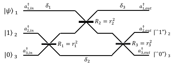
Figure 4: The KLM NLSG using three ordinary beam splitters of reflectivities $R_{i}=r_{i}^{2}$, and optical path delays of $\delta_{i}$. Mode 1 is the primary input state in a weak coherent state (w-CS) containing up to two photons. Mode 2 and 3 are ancilla modes, initially in the state $|1,0\rangle_{23}$. Success of NLPSG is heralded by the detection of the output ancilla modes in their initial state.

$$M_{1}=\left(\begin{array}[]{cc}r_{1}\,e^{i\phi_{1}}&\sqrt{1-r^{2}_{1}}\\ \sqrt{1-r^{2}_{1}}&-r_{1}\,e^{-i\phi_{1}}\\ \end{array}\right),\;M_{2}=\left(\begin{array}[]{cc}-r_{2}\,e^{-i\phi_{2}}&\sqrt{1-r^{2}_{2}}\\ \sqrt{1-r^{2}_{2}}&r_{2}\,e^{i\phi_{2}}\\ \end{array}\right),\;M_{3}=\left(\begin{array}[]{cc}r_{3}\,e^{i\phi_{3}}&\sqrt{1-r^{2}_{3}}\\ \sqrt{1-r^{2}_{3}}&-r_{3}\,e^{-i\phi_{3}}\\ \end{array}\right),$$ (41)

with real BS reflection coefficients $-1\leq r_{i}\leq 1$ (reflectivities $R_{i}=r^{2}_{i}$) . Note that we have chosen a (non-standard) matrix representation of the $2\times 2$ BS matrix that contains only real coefficients Skaar et al. (2004) such that $\det(M_{i})=-1$ for $i\in\{1,2,3\}$.

Recall that a unitary transformation $\mathcal{U}=B_{3}\,B_{2}\,B_{1}$ affects the following transformations on the boson creation operators Skaar et al. (2004); Scott et al. (2019); Alsing and Hach III (2018)

$$a^{\dagger}_{i} \xrightarrow{B_{1}} \sum_{j=1}^{4}\,a^{\dagger}_{j}\,\,(B_{1})_{ji}\xrightarrow{B_{2}}\sum_{j=1}^{4}\,\sum_{k=1}^{4}\,a^{\dagger}_{k}\,(B_{2})_{kj}\,(B_{2})_{ji}\xrightarrow{B_{3}}\sum_{j=1}^{4}\,\sum_{\ell=1}^{4}\,a^{\dagger}_{\ell}\,(B_{3})_{\ell k}\,(B_{2})_{kj}\,(B_{1})_{ji}\equiv\sum_{k=1}^{4}\,a^{\dagger}_{\ell}\,\mathcal{U}_{\ell i},$$ (42)

$$\textrm{with}\quad\mathcal{U}_{\ell i}=\sum_{k=1}^{4}\,\sum_{j=1}^{4}\,(B_{3})_{\ell k}\,(B_{2})_{kj}\,(B_{1})_{ji}\equiv(B_{3}\,B_{2}\,B_{1})_{\ell i},$$

with $B_{1}$ acting first, $B_{2}$ acting second, and $B_{3}$ acting third as we traverse the NLPSG in Fig.(4) from left to right.

Putting the above three blocks together, we have the full evolution from left to right in Fig.(4)

$$\left(\begin{array}[]{c}a^{\dagger}_{1,out}\\ a^{\dagger}_{2,out}\\ a^{\dagger}_{3,out}\\ \end{array}\right)^{T} = \left(\begin{array}[]{c}a^{\dagger}_{1,in}\\ a^{\dagger}_{2,in}\\ a^{\dagger}_{3,in}\\ \end{array}\right)^{T}\,(B_{3}\,B_{2}\,B_{1})\,$$ (43g)

$$= \left(\begin{array}[]{c}a^{\dagger}_{1,in}\\ a^{\dagger}_{2,in}\\ a^{\dagger}_{3,in}\\ \end{array}\right)^{T}\,\left(\begin{array}[]{c|}e^{i\,\delta_{3}}\\ {\begin{array}[]{cc}\hline\cr 0\\[-5.0pt] 0\end{array}}\end{array}\begin{array}[]{cc}0&0\\ \hline\cr{\begin{array}[]{c}\hskip 10.0pt\raisebox{-5.0pt}{${M}_{3}$}\vspace*{15pt}\end{array}}\end{array}\right)\left(\begin{array}[]{c|}\\[-12.50002pt] {M}_{2}\\[8.00003pt] {\begin{array}[]{cc}\hline\cr 0&0\end{array}}\end{array}\begin{array}[]{c}0\\[-3.50006pt] 0\\ {\begin{array}[]{c}\hline\cr e^{i\,\delta_{2}}\end{array}}\end{array}\right)\left(\begin{array}[]{c|}e^{i\,\delta_{1}}\\ {\begin{array}[]{cc}\hline\cr 0\\[-5.0pt] 0\end{array}}\end{array}\begin{array}[]{cc}0&0\\ \hline\cr{\begin{array}[]{c}\hskip 10.0pt\raisebox{-5.0pt}{${M}_{1}$}\vspace*{15pt}\end{array}}\end{array}\right)$$ (43ag)

$$\equiv \left(\begin{array}[]{c}a^{\dagger}_{1,in}\\ a^{\dagger}_{2,in}\\ a^{\dagger}_{2,in}\\ \end{array}\right)^{T}\,S$$ (43ak)

$$= \left(\begin{array}[]{c}a^{\dagger}_{1,in}\\ a^{\dagger}_{2,in}\\ a^{\dagger}_{3,in}\\ \end{array}\right)^{T}\,\left(\begin{array}[]{ccc}S_{11}&S_{12}&S_{13}\\ S_{21}&S_{22}&S_{23}\\ S_{31}&S_{32}&S_{33}\\ \end{array}\right),\,$$ (43ar)

where the superscript $T$ indicates the transpose (i.e. the matrix $\mathcal{U}=B_{3}\,B_{2}\,B_{1}$ acts on the row vector $(a^{\dagger}_{1,in},a^{\dagger}_{2,in},a^{\dagger}_{3,in})$ from the right, as in Eq.(42)). The above product of BS defines the matrix $S$ representing the three mode (1,2,3) KLM NLPSG with components $S_{ij}$ (obtained by explicitly multiplying out $B_{3}\,B_{2}\,B_{1}$) routing a photon initially in mode $j$ (second index) into the mode $i$ (first index). Here, the $\delta_{i}$ represent phase shifts due to the optical path length delays to and from the BSs.

Without loss of generality, we will henceforth only consider the simple case when all phases $\{\phi_{i},\delta_{i}\}$ are identically zero. This yields the $S$-matrix

$$S^{(KLM)}=\left(\begin{array}[]{ccc}-r_{2}&\dfrac{\sqrt{1-r_{2}^{4}}}{\sqrt{1+r_{2}+r_{2}^{2}-3\,r_{2}^{3}}}&\dfrac{\sqrt{1-r_{2}^{2}}\,\sqrt{r_{2}-3\,r_{2}^{3}}}{\sqrt{1+r_{2}+r_{2}^{2}-3\,r_{2}^{3}}}\\ &&\\ \dfrac{\sqrt{1-r_{2}^{4}}}{\sqrt{1+r_{2}+r_{2}^{2}-3\,r_{2}^{3}}}&\dfrac{2\,r_{2}\,(1+r_{2})}{1+2\,r_{2}+3\,r_{2}^{3}}&-\dfrac{\sqrt{1+r_{2}^{2}}\,\sqrt{r_{2}-3\,r_{2}^{3}}}{1+2\,r_{2}+3\,r_{2}^{3}}\\ &&\\ \dfrac{\sqrt{1-r_{2}^{2}}\,\sqrt{r_{2}-3\,r_{2}^{3}}}{\sqrt{1+r_{2}+r_{2}^{2}-3\,r_{2}^{3}}}&-\dfrac{\sqrt{1+r_{2}^{2}}\,\sqrt{r_{2}-3\,r_{2}^{3}}}{1+2\,r_{2}+3\,r_{2}^{3}}&.\dfrac{1+r_{2}+r_{2}^{2}+3\,r_{2}^{3}}{1+2\,r_{2}+3\,r_{2}^{3}}\\ \end{array}\right)$$ (44)

Here we have imposed only Condition-0 and Condition-2 so that $\beta_{0}=\beta_{2}\equiv\beta$ so that

$$r_{1}(r_{2})=r_{3}(r_{2}) = \dfrac{\sqrt{1+r_{2}^{2}}}{\sqrt{(1-r_{2})\,(1+2\,r_{2}+3\,r_{2}^{2})}},$$ (45a)

$$\beta(r_{2}) = \dfrac{2\,r_{2}\,(1+r_{2})}{1+2\,r_{2}+3\,r_{2}^{3}}=S_{22}.$$ (45b)

Maximizing $$\beta r_{2}$$ in Eq.(45b) over yields the optimal operating values Skaar et al. (2004); Scott et al. (2019); Alsing and Hach III (2018)

$$r_{2}^{*} = \sqrt{2}-1\hskip 25.29494pt=0.424214,\qquad r_{2}^{*2}=0.171573,$$ (45c)

$$\textrm{KLM:}\qquad r^{*}_{1}=r^{*}_{3} = \dfrac{1}{\sqrt{4-2\,\sqrt{2}}}\;\;=0.92388,\qquad\;r_{1}^{*2}=r_{3}^{*2}=0.853553,$$ (45d)

$$\beta = \dfrac{1}{2},\qquad\hskip 104.79128pt|\beta|^{2}=\dfrac{1}{4},$$ (45e)

with maximum NLPSG success probability $|\beta|^{2}_{max}=1/4$. Note that due to terms the linear in $r_{2}$ in Eq.(45a) and Eq.(45b) and $r^{2}_{1}(-r_{2})\neq r_{1}^{2}(r_{2})$, we have similarly $|\beta(-r_{2})|^{2}\neq|\beta(-r_{2})|^{2}$. For example, while $|\beta(-r^{*}_{2})|^{2}=1/2$, we have $r^{2}_{1}(-r^{*}_{2})>1$, and hence this unphysical solution must be rejected.

A.2 The MRR NLPSG

We now wish to extend the above considerations for the KLM version of the NLPSG to the MRR version Scott et al. (2019); Alsing and Hach III (2018) by replacing each KLM BS by a MRR. Each MRR_i now has an upper and lower transmission coefficient $\eta_{i},\tau_{i}$, phase angle $\theta_{i}$, and waveguide bus delays $\delta_{i}$ for $i\in\{1,2,3\}$. In Scott et al. (2019); Alsing and Hach III (2018) the authors modeled the solutions of the MRR NLPSG by treating each MRR element as if it had the form of a KLM BS with (now complex) fictitious reflection coefficients $r_{i}$.

The simplest solution was found Scott et al. (2019); Alsing and Hach III (2018) (mimicking a calculation by Skaar Skaar et al. (2004)) by considering the case when all the $\theta_{i}=0$ (i.e. all MRRs on resonance) and all the bus phase delays were also zero $\delta_{i}=0$, so that all the KLM effective reflection coefficients $r_{i}$ were now real. The $S$ matrix for the MRR NLPSG taking $r_{3}=r_{1}$ is given by Scott et al. (2019); Alsing and Hach III (2018)

$$S^{(MRR)}=\dfrac{1}{1-\,(1-r_{1}^{2})\,r_{2}}\,\left(\begin{array}[]{ccc}(1-r_{1}^{2})-r_{2}&r_{1}\,\sqrt{1-r_{2}^{2}}&-r_{1}\,\sqrt{1-r_{1}^{2}}\,\sqrt{1-r_{2}^{1}}\\ r_{1}\,\sqrt{1-r_{2}^{2}}&r_{1}^{2}\,r_{2}&\sqrt{1-r_{1}^{2}}\,(1-r_{2})\\ -r_{1}\,\sqrt{1-r_{1}^{2}}\,\sqrt{1-r_{2}^{1}}&\sqrt{1-r_{1}^{2}}\,(1-r_{2})&r_{1}^{2}\end{array}\right).$$ (46)

The form of $S^{(MRR)}$ now differs from that of the KLM case, only because in the MRR case, the middle photon, mode-$2$ runs backwards (right to left), and so there is some involved mode-swap algebra Scott et al. (2019); Alsing and Hach III (2018) that takes place in forming $S^{(MRR)}$ from $S^{(KLM)}$. As such, it is more compact to write $S^{(MRR)}$ as a function of both $r_{1}$ and $r_{2}$. Analogous to Eq.(45a) and Eq.(45b) we find by imposing only Condition-0 and Condition-2 we have

$$r_{1}(r_{2})=r_{3}(r_{2}) = \left[\dfrac{(1-r_{2})}{r_{2}\,(1+r_{2}^{2})}\,\left((1+2\,r_{2}-r_{2}^{2})\mp(1+r_{2})\,\sqrt{(1-3\,r^{2}_{2})}\right)\right]^{1/2},$$ (47a)

giving rise to

$$\beta(r_{2}) = \left(\dfrac{1}{2\pm\sqrt{1-3\,r_{2}^{2}}}\right)\,\left[\dfrac{1+2\,r_{2}-r_{2}^{2}}{1+r_{2}}\pm\sqrt{1-3\,r_{2}^{2}}\right],$$ (47b)

where in both Eq.(47a) and Eq.(47b) the top sign corresponds to the region $-1/\sqrt{3}\leq r_{2}\leq-1/2$, and the bottom sign to the region $0\leq r_{2}\leq 1/\sqrt{3}$, which are inequivalent solutions. By additionally imposing Condition-1 and maximizing over $r_{2}$ we find analogous to Eq.(45c)

$$r_{2}^{*} = \dfrac{1+2\,\sqrt{2}}{7}\hskip 25.29494pt=0.546918,\qquad r_{2}^{*2}=0.299119,$$ (48a)

$$\textrm{MRR:}\qquad r^{*}_{1}=r^{*}_{3} = \sqrt{2\,(\sqrt{2}-1)}\;\;=0.91018,\qquad\;r_{1}^{*2}=r_{3}^{*2}=0.844778,$$ (48b)

$$\beta = \dfrac{1}{2},\qquad\hskip 108.405pt|\beta|^{2}=\dfrac{1}{4},$$ (48c)

with maximum NLPSG success probability $|\beta|^{2}_{max}=1/4$.

The difference between the analysis in Scott et al. (2019); Alsing and Hach III (2018) and in this present work is that here we also want to consider the case of cl-SPDC input states (only containing the states $|0\rangle_{k\in\{1,4\}}$ and $|2\rangle_{k\in\{1,4\}}$), in addition to the full w-CS input states (also containing the states $|1\rangle_{k\in\{1,4\}}$). In the case of cl-SPDC input states, we will find that not imposing Condition-1, namely not letting $\beta_{1}$ to be equal necessarily to $\beta$ (now defined by imposing only Condition-0 and Condition-2) gives qualitatively the same coincidence interference curves. More importantly, the MRR solutions for the fictitious KLM reflections coefficients $r^{*}_{i}$ define a 1-parameter family of physical transmission coefficients $\eta_{i}~{}=~{}\eta_{i}(\tau_{i};r^{*}_{i})$ regardless of the value of $|\beta|^{2}$ associated with the chosen value of $r^{*}_{i}$

$$\eta_{i}(\tau_{i};r^{*}_{i})=\dfrac{r^{*}_{i}+\tau_{i}}{1+r^{*}_{i}\,\tau_{i}},\quad|\tau_{i}|\leq 1\Rightarrow|\eta_{i}|\leq 1,\quad\textrm{for fixed}\quad|r^{*}_{i}|\leq 1,$$ (49)

as illustrated in Fig.(5) for values of $r_{1}^{*2}$ and $r_{2}^{*2}$ yielding $\beta^{2}=1/4$ for both the KLM-NLPSG and MRR-NLPSG.

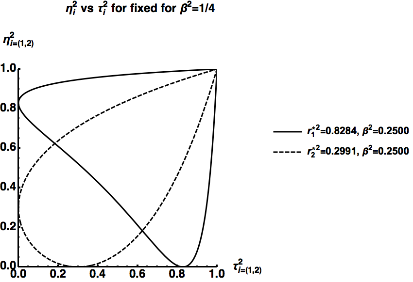
Figure 5: Plots of the physical MRR transmissivities (solid) $\eta^{2}_{1=3}$ vs $\tau^{2}_{1=3}$, and (dashed) $\eta^{2}_{2}$ vs $\tau^{2}_{2}$ for fixed values of the fictitious KLM reflectivities $r^{*2}_{2}$ yielding $\beta^{2}=1/4$. (Fig.(3) repeated here for clarity).

The analysis for the case of MRR runs similarly for the KLM case by merely replacing $S^{(KLM)}\to S^{(MRR)}$ in the unitary matrix $\mathcal{U}$. The values of $r^{*}_{i}$ now differ from the KLM case, only because in the MRR case, the middle photon, mode-$2$ runs backwards, and so there is some mode-swap algebra that takes place in forming $S^{(MRR)}$ from $S^{(KLM)}$.

Appendix B Action of the BS on $|n,m\rangle_{ab}$

We need to know how an ideal, lossless BS acts on an arbitrary input state $|n,m\rangle$ presented at its two input ports. Let us define the BS transformation (Hamiltonian) on two modes $a$ and $b$ as $BS=(\theta/2)\,(a\,b^{\dagger}+a^{\dagger}\,b)$. Here $R\equiv\sin^{2}(\theta/2)$ is the reflectivity and $T=(1-R)=\cos^{2}(\theta/2)$ is the transmissivity, such that $R+T=1$, as shown in Fig.(6). (Note: we call the quantities $\sin(\theta/2)$ and $\cos(\theta/2)$ reflection and transmission coefficients). The factor of $1/2$ in the argument $\theta/2$ is introduced so that $\theta=\pi/2$ represents a 50:50 BS.

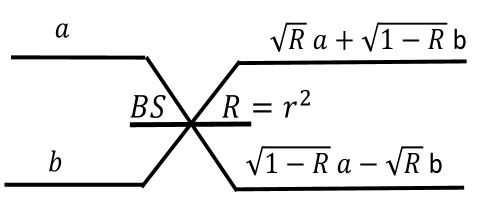
Figure 6: Two optical modes $a$ and $b$ mixing on a BS of reflectivity $R$. Note that in this (not always standard) representation the $a_{in}$ mode is the top-left input, while the $a_{out}$ mode is defined via where $a_{in}$ transmits to, i.e. as the lower right output. Similarly for $b_{in}$ and $b_{out}$. Here, the bottom of the BS imparts a $\pi$ phase shift of $-1$ upon reflection.

The action of the BS on an arbitrary input of Fock states $|n\rangle_{a}|m\rangle_{b}\equiv\dfrac{(a^{\dagger})^{n}}{\sqrt{n!}}\,\dfrac{(b^{\dagger})^{n}}{\sqrt{m!}}\,|0\rangle_{a}|0\rangle_{b}$ is straightforwardly computed (see Chapter 5 of Agarwal Quantum Optics Agarwal (2013)) by applying the BS transformation to the last expression, and expanding out terms using the binomial theorem (since $a^{\dagger}$ and $b^{\dagger}$ commute). Note that if we write the BS transformation $S_{BS}$ of the out operators in terms of the in operators as $\vec{a}^{\dagger}_{out}=S_{BS}\,\vec{a}^{\dagger}_{in}$ then to transform an input state such as $|1\rangle_{a}\,|0\rangle_{b}=a^{\dagger}_{in}|0\rangle_{a}\,|0\rangle_{b}$, we need to write the in operators in terms of the out operators using the transpose transformation $S^{T}_{BS}$ as $\vec{a}^{\dagger}_{in}=S^{T}_{BS}\,\vec{a}^{\dagger}_{out}$ via

$$\vec{a}^{\dagger}_{out}=\left[\begin{array}[]{c}a^{\dagger}_{out}\\ b^{\dagger}_{out}\end{array}\right]=\left[\begin{array}[]{cc}\cos(\theta/2)&-\sin(\theta/2)\\ \sin(\theta/2)&\cos(\theta/2)\end{array}\right]\,\left[\begin{array}[]{c}a^{\dagger}_{in}\\ b^{\dagger}_{in}\end{array}\right]\equiv S_{BS}\,\vec{a}^{\dagger}_{in}\Rightarrow\vec{a}^{\dagger}_{in}=S^{T}_{BS}\,\vec{a}^{\dagger}_{out}.$$ (50)

Thus, for example $a^{\dagger}_{in}|0\rangle_{a}\,|0\rangle_{b}\to\left(\cos(\theta/2)\,a^{\dagger}_{out}+\sin(\theta/2)\,b^{\dagger}_{out}\right)\,|0\rangle_{a}\,|0\rangle_{b}=\cos(\theta/2)\,|1\rangle_{a}\,|0\rangle_{b}+\sin(\theta/2)|0\rangle_{a}\,|1\rangle_{b}$. We can drop all the in, out labels and just remember to use the transformation $S^{T}_{BS}$ in computing the BS transformation formula. The derivation is easily carried out (see also Agarwal Agarwal (2013)) with the results given below using $S^{T}_{BS}$ to transform an input state $|n\rangle_{a}|m\rangle_{b}$ to an output state, yielding

$$|n\rangle_{a}|m\rangle_{b}\to\sum_{p=0}^{n+m}\,f^{(n,m)}_{p}\,|p\rangle_{a}\,|n+m-p\rangle_{b},,$$ (51)

$$f^{(n,m)}_{p}=\sum_{q=0}^{n}\sum_{q^{\prime}=0}^{m}\delta_{p,q+q^{\prime}}\,\binom{n}{q}\,\binom{m}{q^{\prime}}\,\sqrt{\dfrac{p!\,(n+m-p)!}{n!\,m!}}\,\left(-1\right)^{q^{\prime}}\,\left(\cos(\theta/2)\right)^{m+q-q^{\prime}}\,\left(\sin(\theta/2)\right)^{n-q+q^{\prime}}.\qquad$$ (52)

Note that the delta function $\delta_{p,q+q^{\prime}}$ ensures that the BS mixes the original input state $|n\rangle_{a}|m\rangle_{b}$ only amongst the $n+m+1$ states of total photon number $n+m$ of the form $\{|0\rangle_{a}|n+m\rangle_{b},\,|1\rangle_{a}|n+m-1\rangle_{b},\ldots|n\rangle_{a}|m\rangle_{b},\ldots,|n+m-1\rangle_{a}|1\rangle_{b},\ |n+m\rangle_{a}|0\rangle_{b}\}$. The (real) BS coefficients $f^{(n,m)}_{p}$ are easily worked out by hand by considering states $|n\rangle_{a}|m\rangle_{b}$ up to $n+m=2$ at the input ports of BS, namely:

$$p=0:$$

$$|0\rangle_{a}|0\rangle_{b} \to |0\rangle_{a}|0\rangle_{b}\Rightarrow f^{(0,0)}_{0}=1,$$ (53a)

$$p=1:$$

$$|0\rangle_{a}|1\rangle_{b} \to [\cos(\theta/2)\,b-\sin(\theta/2)\,a]|0\rangle_{a}|0\rangle_{b},$$ (53d)

$$= \cos(\theta/2)|0\rangle_{a}|1\rangle_{b}-\sin(\theta/2)|1\rangle_{a}|0\rangle_{b},\Rightarrow\left\{\begin{array}[]{ccr}f^{(0,1)}_{0}&=&\cos(\theta/2)\\ f^{(0,1)}_{1}&=&-\sin(\theta/2)\end{array}\right.$$

$$|1\rangle_{a}|0\rangle_{b} \to [\cos(\theta/2)\,a+\sin(\theta/2)\,b]|0\rangle_{a}|0\rangle_{b},$$ (53g)

$$= \sin(\theta/2)|0\rangle_{a}|1\rangle_{b}+\cos(\theta/2)|1\rangle_{a}|0\rangle_{b},\Rightarrow\left\{\begin{array}[]{ccr}f^{(1,0)}_{0}&=&\sin(\theta/2),\\ f^{(1,0)}_{1}&=&\cos(\theta/2),\end{array}\right.$$

$$p=2:$$

$$|0\rangle_{a}|2\rangle_{b} = \dfrac{1}{\sqrt{2}}\,b^{2}\,|0\rangle_{a}|0\rangle_{b}\to\dfrac{1}{\sqrt{2}}\,[\cos(\theta/2)\,b-\sin(\theta/2)\,a]^{2}|0\rangle_{a}|0\rangle_{b},$$ (53l)

$$= \cos^{2}(\theta/2)|0\rangle_{a}|2\rangle_{b}-\sin(\theta)|1\rangle_{a}|1\rangle_{b}+\sin^{2}(\theta/2)|2\rangle_{a}|0\rangle_{b},\Rightarrow\left\{\begin{array}[]{ccl}f^{(0,2)}_{0}&=&\cos^{2}(\theta/2),\\ f^{(0,2)}_{1}&=&-\frac{1}{\sqrt{2}}\,\sin(\theta),\\ f^{(0,2)}_{2}&=&\sin^{2}(\theta/2),\end{array}\right.$$

$$|1\rangle_{a}|1\rangle_{b} = a\,b\,|0\rangle_{a}|0\rangle_{b}\to[\cos(\theta/2)\,a+\sin(\theta/2)\,b]\,[\cos(\theta/2)\,b-\sin(\theta/2)\,a]|0\rangle_{a}|0\rangle_{b},$$ (53p)

$$= \sqrt{2}\,\sin(\theta/2)\,\cos(\theta/2)|0\rangle_{a}|2\rangle_{b}[\cos^{2}(\theta/2)-\sin^{2}(\theta/2)]|1\rangle_{a}|1\rangle_{b},$$

$$\hskip 126.47249pt-\sqrt{2}\sin(\theta/2)\,\cos(\theta/2)|2\rangle_{a}|0\rangle_{b},\Rightarrow\left\{\begin{array}[]{ccl}f^{(1,1)}_{0}&=&\frac{1}{\sqrt{2}}\sin(\theta),\\ f^{(1,1)}_{1}&=&\cos(\theta),\\ f^{(1,1)}_{2}&=&-\frac{1}{\sqrt{2}}\sin(\theta),\end{array}\right.$$

$$|2\rangle_{a}|0\rangle_{b} = \dfrac{1}{\sqrt{2}}\,a^{2}\,|0\rangle_{a}|0\rangle_{b}\to\dfrac{1}{\sqrt{2}}\,[\cos(\theta/2)\,a+\sin(\theta/2)\,b]^{2}|0\rangle_{a}|0\rangle_{b},$$ (53t)

$$= \sin^{2}(\theta/2)|0\rangle_{a}|2\rangle_{b}+\sin(\theta)|1\rangle_{a}|1\rangle_{b}+\cos^{2}(\theta/2)|2\rangle_{a}|0\rangle_{b},\Rightarrow\left\{\begin{array}[]{ccl}f^{(2,0)}_{0}&=&\sin^{2}(\theta/2),\\ f^{(2,0)}_{1}&=&\frac{1}{\sqrt{2}}\,\sin(\theta),\\ f^{(2,0)}_{2}&=&\cos^{2}(\theta/2),\end{array}\right.\qquad$$

Note: for each $(n,m)$ we have $\sum_{p=0}^{n+m}|f^{(n,m)}_{p}|^{2}=1$, which just indicates that the BS transformation is unitary. Note that the $f^{(n,m)}_{p}$ are just the Wigner rotation coefficients for the representation of a system with spin $J=(n+m)/2$ in the angular momentum basis $|J,M\rangle$ with $2J+1=n+m+1$ states $M\in\{-J,-J+1,\ldots,J\}$ where $M(p)=-J+p\,(2J)/(n+m)$ for $p\in\{0,\ldots,n+m\}$.

Appendix C $\mathcal{U}$ coefficients for the 4- and 5-photon accidental states

C.1 The 5-photon accidental states

The 5-photon state $|T_{2,2^{\prime}}\rangle_{1234}$ in Eq.(21a) proportional to ${\alpha}_{2}\,{\alpha}^{\prime}_{2}\,e^{i\,2\,\varphi}$ contributes accidentals (noise terms) to the primary coincidence counts by transferring (rerouting) photons into states that will be counted as coincidence counts under finite detection efficiencies. These states arise via the BS interaction on mode $1$ and $4$. These accidentals states do not contribute to the primary interference terms since they are all part of $|\psi^{\perp}_{out}\rangle$ and hence are orthogonal to $|1,1,0,1\rangle_{1234}$ upon which the primary coincidence interference effect takes place. Further, since each orthogonal state is multiplied by an overall phase factor $e^{i\,2\,\varphi}$, this phase factor squares to unity in the final probability sum, and hence does not even interfere, in higher order, with other states in $|\psi^{\perp}_{out}\rangle$. Note also that these accidentals involve states with a total photon number of $5$, while the primary coincidence interfering terms contain a total of $3$ photons. So our approximation would see a pure coincidence interference pattern if we were to stop at the $3$-photon level. However, since our initial input state is already a $5$-photon state, a reasonable self consistent, lowest order calculation would be to consider states with up to $5$ photons, as we do here.

The total number of $5$-photon Fock states in $|T_{2,2^{\prime}}\rangle$ Eq.(21a) is $4^{3}\times 3=192$ (4 creation operators in each of 3 sums, and 3 terms from expanding the square of the BS operation on mode 4). To get a handle on what terms to keep, it is useful to indicate the possible boson creation operator indices $a^{\dagger}_{j}\,a^{\dagger}_{k}\,a^{\dagger}_{\ell}$ as $(j)[k,\ell](1,1)$, $(j)[k,\ell](4,4)$ and $(j)[k,\ell](1,4)$ where the last set of indices in parentheses indicate the terms $(a^{\dagger}_{1})^{2}$, $(a^{\dagger}_{4})^{2}$ and $a^{\dagger}_{1}\,a^{\dagger}_{4}$ from the expansion of the BS on mode-$4$. Consider the first set of indices $(1)[k,\ell](11)$. These can be completely eliminated since it contains three $1$s corresponding to a state $|3,\cdot,\cdot,\cdot\rangle_{1234}$ which is outside our approximation which keeps terms with at most two photons in any single mode.

For the next set of indices $(2)[k,\ell](11)$ we observe that since there already exists two $1$s and one $2$, the indices $[k,\ell]$ cannot contain a $1$ (since that would give three photons in mode-$1$), nor can it contain $[k,\ell]=[2,2]$ (since that would give a state with three photons in mode-$2$). Further, the contributing indices must contain as a subset, the indices $\{1,2,4\}$ since terms that don’t are multiplied by $p^{(1,2,4)}_{0}=0$. Thus the $5$ contributing index sets are given by $(2)\{[2,4],[3,4],[4,2],[4,3],[4,4]\}(11)$ corresponding to state $\{|2,2,0,1\rangle_{1234},|2,1,1,1\rangle_{1234},|2,2,0,1\rangle_{1234},|2,1,1,1\rangle_{1234},|2,1,0,2\rangle_{1234},\}$, respectively (e.g. $(2)[2,4](11)$ is read off as (11) two photons in mode-$1$, (22) two photons in mode-$2$, and (4) one photon in mode-$4$).

Note that the next set of indices in line $(3)[k,\ell](11)$ only contains two terms $[k,\ell]=\{[2,4],[4,2]\}$ since all dropped terms either do not contain $\{1,2,4\}$, or contains $[k,\ell]=[3,3]$ which yields three photons in mode-$3$.

Similar to the prior case, the set of contributing indices for $(4)[k,\ell](11)$ are $(4)\{[2,2],[2,3],[2,4],[3,2],[4,2]\}(11)$ corresponding to state $\{|2,2,0,1\rangle_{1234},|2,1,1,1\rangle_{1234},|2,1,0,2\rangle_{1234},|2,1,1,1\rangle_{1234},|2,1,0,2\rangle_{1234},\}$, respectively. We can proceed similarly with the $(j)[k,\ell](44)$ and $(j)[k,\ell](14)$, noting right off the bat that we can eliminate the set of indices $(4)[k,\ell](44)$ since it contains three photons in mode-$4$. The process is an exercise in tedious bookkeeping, but the procedure is straightforward, and yields (note: $\{cc,cs,ss\}$ superscripts indicate terms are multiplied by $\{\cos^{2}(\theta/2),2\,\cos(\theta/2)\sin(\theta/2),\sin^{2}(\theta/2)\}$)

$$|T_{2,2^{\prime}}\rangle_{1234} = {\alpha}_{2}\,{\alpha}^{\prime}_{2}\,e^{i\,2\,\varphi}\times$$ (54)

$$|1,2,0,2\rangle_{1234}\,\left[\sin(\theta)\,\mathcal{U}^{(cs)}_{202}+\sin^{2}(\theta/2)\,\mathcal{U}^{(ss)}_{202}\right],$$

$$+ |1,2,1,1\rangle_{1234}\,\left[\sin(\theta)\,\mathcal{U}^{(cs)}_{211}\right],$$

$$+ |1,1,1,2\rangle_{1234}\,\left[\sin(\theta)\,\mathcal{U}^{(cs)}_{112}+\sin^{2}(\theta/2)\,\mathcal{U}^{(ss)}_{112}\right],$$

$$+ |1,1,2,1\rangle_{1234}\,\left[\sin(\theta)\,\mathcal{U}^{(cs)}_{121}\right],$$

$$+ |2,2,0,1\rangle_{1234}\,\left[\cos^{2}(\theta/2)\,\mathcal{U}^{(cc)}_{201}+\sin(\theta)\,\mathcal{U}^{(cs)}_{201}\right],$$

$$+ |2,1,1,1\rangle_{1234}\,\left[\cos^{2}(\theta/2)\,\mathcal{U}^{(cc)}_{111}+\sin(\theta)\,\mathcal{U}^{(cs)}_{111}\right],$$

$$+ |2,1,0,2\rangle_{1234}\,\left[\cos^{2}(\theta/2)\,\mathcal{U}^{(cc)}_{102}+\sin(\theta)\,\mathcal{U}^{(cs)}_{102}+\sin^{2}(\theta/2)\,\mathcal{U}^{(ss)}_{102}\right],$$

where we have defined the coefficients of the $|1\rangle_{1}\otimes|\cdot,\cdot,\cdot\rangle_{234}$ terms as

$$\mathcal{U}^{(cs)}_{202} = \left(\mathcal{U}_{21}\,\mathcal{U}_{21}\,\mathcal{U}_{42}+\mathcal{U}_{21}\,\mathcal{U}_{41}\,\mathcal{U}_{22}\right),$$ (55a)

$$\mathcal{U}^{(cs)}_{211} = \frac{1}{\sqrt{2}}\,\left(\mathcal{U}_{21}\,\mathcal{U}_{31}\,\mathcal{U}_{22}+\mathcal{U}_{31}\,\mathcal{U}_{21}\,\mathcal{U}_{22}\right),$$ (55b)

$$\mathcal{U}^{(cs)}_{112} = \frac{1}{\sqrt{2}}\,\left(\mathcal{U}_{21}\,\mathcal{U}_{31}\,\mathcal{U}_{42}+\mathcal{U}_{21}\,\mathcal{U}_{41}\,\mathcal{U}_{32}+\mathcal{U}_{31}\,\mathcal{U}_{21}\,\mathcal{U}_{42}+\mathcal{U}_{31}\,\mathcal{U}_{41}\,\mathcal{U}_{22}+\mathcal{U}_{41}\,\mathcal{U}_{21}\,\mathcal{U}_{32}+\mathcal{U}_{41}\,\mathcal{U}_{31}\,\mathcal{U}_{22}\right),\qquad\;$$ (55c)

$$\mathcal{U}^{(cs)}_{121} = \frac{1}{\sqrt{2}}\,\left(\mathcal{U}_{21}\,\mathcal{U}_{31}\,\mathcal{U}_{32}+\mathcal{U}_{31}\,\mathcal{U}_{21}\,\mathcal{U}_{32}+\mathcal{U}_{31}\,\mathcal{U}_{31}\,\mathcal{U}_{22}\right),$$ (55d)

$$\mathcal{U}^{(ss)}_{112} = \left(\mathcal{U}_{11}\,\mathcal{U}_{21}\,\mathcal{U}_{32}+\mathcal{U}_{11}\,\mathcal{U}_{31}\,\mathcal{U}_{22}+\mathcal{U}_{21}\,\mathcal{U}_{11}\,\mathcal{U}_{32}+\mathcal{U}_{21}\,\mathcal{U}_{31}\,\mathcal{U}_{12}\right),$$ (55e)

$$\mathcal{U}^{(ss)}_{202} = \left(\mathcal{U}_{31}\,\mathcal{U}_{21}\,\mathcal{U}_{22}+\mathcal{U}_{21}\,\mathcal{U}_{11}\,\mathcal{U}_{22}+\mathcal{U}_{21}\,\mathcal{U}_{21}\,\mathcal{U}_{12}\right),$$ (55f)

with $\mathcal{U}$ defined from Eq.(18). (Note that the second indices of the triple products of $\mathcal{U}$s are always in the order $\{1,1,2\}$; the first set of indices $\{j,k,\ell\}$ are associated with the state $|j,k,\ell\rangle_{234}$) Similarly, the coefficients of the $|2\rangle_{1}\otimes|\cdot,\cdot,\cdot\rangle_{234}$ terms are given by

$$\mathcal{U}^{(cc)}_{201} = \left(\mathcal{U}_{21}\,\mathcal{U}_{21}\,\mathcal{U}_{24}+\mathcal{U}_{21}\,\mathcal{U}_{41}\,\mathcal{U}_{22}+\mathcal{U}_{41}\,\mathcal{U}_{21}\,\mathcal{U}_{22}\right),$$ (56a)

$$\mathcal{U}^{(cc)}_{111} = \frac{1}{\sqrt{2}}\,\left(\mathcal{U}_{21}\,\mathcal{U}_{31}\,\mathcal{U}_{42}+\mathcal{U}_{21}\,\mathcal{U}_{41}\,\mathcal{U}_{32}+\mathcal{U}_{41}\,\mathcal{U}_{31}\,\mathcal{U}_{22}\right),$$ (56b)

$$\mathcal{U}^{(cc)}_{102} = \left(\mathcal{U}_{21}\,\mathcal{U}_{41}\,\mathcal{U}_{42}+\mathcal{U}_{41}\,\mathcal{U}_{41}\,\mathcal{U}_{22}+\mathcal{U}_{41}\,\mathcal{U}_{41}\,\mathcal{U}_{22}\right),$$ (56c)

$$\mathcal{U}^{(cs)}_{201} = \left(\mathcal{U}_{11}\,\mathcal{U}_{21}\,\mathcal{U}_{22}+\mathcal{U}_{21}\,\mathcal{U}_{11}\,\mathcal{U}_{22}+\mathcal{U}_{21}\,\mathcal{U}_{21}\,\mathcal{U}_{12}\right),$$ (56d)

$$\mathcal{U}^{(cs)}_{111} = \frac{1}{\sqrt{2}}\,\left(\mathcal{U}_{11}\,\mathcal{U}_{21}\,\mathcal{U}_{32}+\mathcal{U}_{11}\,\mathcal{U}_{31}\,\mathcal{U}_{22}\right)+\left(\mathcal{U}_{21}\,\mathcal{U}_{11}\,\mathcal{U}_{32}+\mathcal{U}_{11}\,\mathcal{U}_{21}\,\mathcal{U}_{32}+\mathcal{U}_{21}\,\mathcal{U}_{31}\,\mathcal{U}_{12}\right),$$ (56e)

$$+ \frac{1}{\sqrt{2}}\,\left(\mathcal{U}_{31}\,\mathcal{U}_{11}\,\mathcal{U}_{22}+\mathcal{U}_{31}\,\mathcal{U}_{21}\,\mathcal{U}_{12}\right),$$

$$\mathcal{U}^{(cs)}_{102} = \left(\mathcal{U}_{11}\,\mathcal{U}_{21}\,\mathcal{U}_{42}+\mathcal{U}_{11}\,\mathcal{U}_{41}\,\mathcal{U}_{22}+\mathcal{U}_{21}\,\mathcal{U}_{11}\,\mathcal{U}_{42}+\mathcal{U}_{21}\,\mathcal{U}_{41}\,\mathcal{U}_{12}+\mathcal{U}_{41}\,\mathcal{U}_{11}\,\mathcal{U}_{22}+\mathcal{U}_{41}\,\mathcal{U}_{21}\,\mathcal{U}_{12}\right),\qquad$$ (56f)

$$\mathcal{U}^{(ss)}_{102} = \left(\mathcal{U}_{11}\,\mathcal{U}_{11}\,\mathcal{U}_{22}+\mathcal{U}_{11}\,\mathcal{U}_{21}\,\mathcal{U}_{12}+\mathcal{U}_{21}\,\mathcal{U}_{11}\,\mathcal{U}_{12}\right).$$ (56g)

C.2 The 4-photon accidental states when $|1\rangle_{1}$ and $|1\rangle_{4}$ are included in the input states

Following the same procedure as in the previous section, the coincidence state after projection, will be (note: $\{cc,cs,ss,\}$ superscripts indicate terms are multiplied by $\{\cos^{2}(\theta/2),2\,\cos(\theta/2)\sin(\theta/2),\sin^{2}(\theta/2)\}$ and $\{c,s\}$ superscripts indicate terms are multiplied by $\{\cos(\theta/2),2\,\sin(\theta/2)\}$)

$$|T_{1,1^{\prime}}\rangle_{1234} + |T_{1,2^{\prime}}\rangle_{1234}+|T_{2,1^{\prime}}\rangle_{1234}=$$ (57)

$${\alpha}_{1}\,{\alpha}^{\prime}_{1}\,e^{i\,\varphi}\,|1,1,0,1\rangle_{1234}\,\left[\cos(\theta/2)\,\mathcal{U}^{\prime(c)}_{101}+\sin(\theta/2)\,\mathcal{U}^{\prime(s)}_{101}\,\right]$$

$$+\,e^{i\,\varphi}\,|1,2,0,1\rangle_{1234}\,\left[{\alpha}_{1}\,{\alpha}^{\prime}_{2}\,e^{i\,\varphi}\,\sin(\theta)\,\mathcal{U}^{\prime(cs)}_{201}+{\alpha}_{2}\,{\alpha}^{\prime}_{1}\,\left(\cos(\theta/2)\,\mathcal{U}^{\prime(c)}_{201}+\sin(\theta/2)\,\mathcal{U}^{\prime(s)}_{201}\right)\right],$$

$$+\,e^{i\,\varphi}\,|1,1,1,1\rangle_{1234}\,\left[{\alpha}_{1}\,{\alpha}^{\prime}_{2}\,e^{i\,\varphi}\,\sin(\theta)\,\mathcal{U}^{\prime(cs)}_{111}+{\alpha}_{2}\,{\alpha}^{\prime}_{1}\,\left(\cos(\theta/2)\,\mathcal{U}^{\prime(c)}_{111}+\sin(\theta/2)\,\mathcal{U}^{\prime(s)}_{111}\right)\right],$$

$$+\,e^{i\,\varphi}\,|1,1,0,2\rangle_{1234}\,\left[{\alpha}_{1}\,{\alpha}^{\prime}_{2}\,e^{i\,\varphi}\,\left(\sin(\theta)\,\mathcal{U}^{\prime(cs)}_{102}+\cos^{2}(\theta/2)\,\mathcal{U}^{\prime(cc)}_{102}\right)+{\alpha}_{2}\,{\alpha}^{\prime}_{1}\,\left(\cos(\theta/2)\,\mathcal{U}^{\prime(c)}_{102}+\sin(\theta/2)\,\mathcal{U}^{\prime(s)}_{102}\right)\right],$$

$$+\,e^{i\,\varphi}\,|2,1,0,1\rangle_{1234}\,\left[{\alpha}_{1}\,{\alpha}^{\prime}_{2}\,e^{i\,\varphi}\,\left(\sin(\theta)\,\mathcal{U}^{\prime(cs)}_{101}+\sin^{2}(\theta/2)\,\mathcal{U}^{\prime(ss)}_{101}\right)+{\alpha}_{2}\,{\alpha}^{\prime}_{1}\,\left(\cos(\theta/2)\,\mathcal{U}^{\prime(c)}_{101}+\sin(\theta/2)\,\mathcal{U}^{\prime(s)}_{101}\right)\right],\qquad\;\;$$

where (Note: all double products $\mathcal{U}\,\mathcal{U}$ have the second indices in the order $\{1,2\}$, while again all triple products $\mathcal{U}\,\mathcal{U}\,\mathcal{U}$ have the second indices in the order $\{1,1,2\}$)

$$\mathcal{U}^{\prime(c)}_{101} = \mathcal{U}_{11}\,\mathcal{U}_{22}+\mathcal{U}_{21}\,\mathcal{U}_{12}=\cos(\theta/2)\,(S_{11}\,S_{22}+S_{21}\,S_{12})\equiv\cos(\theta/2)\,\beta_{1},$$ (58a)

$$\mathcal{U}^{\prime(s)}_{101} = \mathcal{U}_{21}\,\mathcal{U}_{42}+\mathcal{U}_{41}\,\mathcal{U}_{22}=-\sin(\theta/2)\,(S_{21}\,S_{22}+S_{11}\,S_{22})\equiv-\sin(\theta/2)\,\beta_{1},$$ (58b)

$$\mathcal{U}^{\prime(cs)}_{201} = \mathcal{U}_{21}\,\mathcal{U}_{22}$$ (58c)

$$\mathcal{U}^{\prime(cs)}_{111} = \dfrac{1}{\sqrt{2}}\,\left(\mathcal{U}_{21}\,\mathcal{U}_{32}+\mathcal{U}_{31}\,\mathcal{U}_{22}\right),$$ (58d)

$$\mathcal{U}^{\prime(cs)}_{102} = \mathcal{U}_{21}\,\mathcal{U}_{42}+\mathcal{U}_{41}\,\mathcal{U}_{22}=-\sin(\theta/2)\,(S_{21}\,S_{12}+S_{11}\,S_{22})\equiv-\sin(\theta/2)\,\beta_{1},$$ (58e)

$$\mathcal{U}^{\prime(cs)}_{101} = \mathcal{U}_{11}\,\mathcal{U}_{22}+\mathcal{U}_{21}\,\mathcal{U}_{12}=\cos(\theta/2)\,(S_{11}\,S_{22}+S_{21}\,S_{12})\equiv\cos(\theta/2)\,\beta_{1},$$ (58f)

$$\mathcal{U}^{\prime(cc)}_{102} = \mathcal{U}_{11}\,\mathcal{U}_{22}+\mathcal{U}_{21}\,\mathcal{U}_{12}=\cos(\theta/2)\,(S_{11}\,S_{22}+S_{21}\,S_{12})\equiv\cos(\theta/2)\,\beta_{1},$$ (58g)

$$\mathcal{U}^{\prime(ss)}_{101} = \mathcal{U}_{21}\,\mathcal{U}_{42}+\mathcal{U}_{41}\,\mathcal{U}_{22}=-\sin(\theta/2)\,(S_{21}\,S_{12}+S_{11}\,S_{22})\equiv-\sin(\theta/2)\,\beta_{1},$$ (58h)

$$\mathcal{U}^{\prime(c)}_{201} = \mathcal{U}_{11}\,\mathcal{U}_{21}\,\mathcal{U}_{22}+\mathcal{U}_{21}\,\mathcal{U}_{11}\,\mathcal{U}_{22}+\mathcal{U}_{21}\,\mathcal{U}_{21}\,\mathcal{U}_{12},$$ (58i)

$$\mathcal{U}^{\prime(c)}_{111} = \dfrac{1}{\sqrt{2}}\,\left(\mathcal{U}_{11}\,\mathcal{U}_{21}\,\mathcal{U}_{32}+\mathcal{U}_{11}\,\mathcal{U}_{31}\,\mathcal{U}_{22}+\mathcal{U}_{21}\,\mathcal{U}_{11}\,\mathcal{U}_{32}+\mathcal{U}_{21}\,\mathcal{U}_{31}\,\mathcal{U}_{12}+\mathcal{U}_{31}\,\mathcal{U}_{11}\,\mathcal{U}_{22}+\mathcal{U}_{31}\,\mathcal{U}_{21}\,\mathcal{U}_{12}\right),\qquad\;$$ (58j)

$$\mathcal{U}^{\prime(c)}_{102} = \mathcal{U}_{11}\,\mathcal{U}_{21}\,\mathcal{U}_{42}+\mathcal{U}_{11}\,\mathcal{U}_{41}\,\mathcal{U}_{22}+\mathcal{U}_{21}\,\mathcal{U}_{11}\,\mathcal{U}_{42}+\mathcal{U}_{21}\,\mathcal{U}_{41}\,\mathcal{U}_{12}+\mathcal{U}_{41}\,\mathcal{U}_{11}\,\mathcal{U}_{22}+\mathcal{U}_{41}\,\mathcal{U}_{21}\,\mathcal{U}_{12}$$ (58k)

$$\mathcal{U}^{\prime(c)}_{101} = \mathcal{U}_{11}\,\mathcal{U}_{11}\,\mathcal{U}_{22}+\mathcal{U}_{11}\,\mathcal{U}_{21}\,\mathcal{U}_{12}+\mathcal{U}_{21}\,\mathcal{U}_{11}\,\mathcal{U}_{12},$$ (58l)

$$\mathcal{U}^{\prime(s)}_{201} = \mathcal{U}_{21}\,\mathcal{U}_{21}\,\mathcal{U}_{42}+\mathcal{U}_{21}\,\mathcal{U}_{41}\,\mathcal{U}_{22}+\mathcal{U}_{41}\,\mathcal{U}_{21}\,\mathcal{U}_{22},$$ (58m)

$$\mathcal{U}^{\prime(s)}_{111} = \dfrac{1}{\sqrt{2}}\,\left(\mathcal{U}_{21}\,\mathcal{U}_{31}\,\mathcal{U}_{42}+\mathcal{U}_{21}\,\mathcal{U}_{41}\,\mathcal{U}_{32}+\mathcal{U}_{31}\,\mathcal{U}_{21}\,\mathcal{U}_{42}+\mathcal{U}_{31}\,\mathcal{U}_{41}\,\mathcal{U}_{22}+\mathcal{U}_{41}\,\mathcal{U}_{21}\,\mathcal{U}_{32}+\mathcal{U}_{41}\,\mathcal{U}_{31}\,\mathcal{U}_{22}\right),\qquad\;$$ (58n)

$$\mathcal{U}^{\prime(s)}_{102} = \mathcal{U}_{21}\,\mathcal{U}_{41}\,\mathcal{U}_{42}+\mathcal{U}_{41}\,\mathcal{U}_{21}\,\mathcal{U}_{42}+\mathcal{U}_{41}\,\mathcal{U}_{41}\,\mathcal{U}_{22},$$ (58o)

$$\mathcal{U}^{\prime(s)}_{101} = \mathcal{U}_{11}\,\mathcal{U}_{21}\,\mathcal{U}_{42}+\mathcal{U}_{11}\,\mathcal{U}_{41}\,\mathcal{U}_{22}+\mathcal{U}_{21}\,\mathcal{U}_{11}\,\mathcal{U}_{42}+\mathcal{U}_{21}\,\mathcal{U}_{41}\,\mathcal{U}_{12}+\mathcal{U}_{41}\,\mathcal{U}_{11}\,\mathcal{U}_{22}+\mathcal{U}_{41}\,\mathcal{U}_{21}\,\mathcal{U}_{12}.$$ (58p)

In the above we have defined as in Eq.(7b)

$$\beta_{1}\equiv S_{11}\,S_{22}+S_{21}\,S_{12}\hbox{ \raise-5.69054pt\hbox{$\textstyle{\longrightarrow}\atop\scriptstyle{\beta\to\beta_{max}=1/2}$} }\,\beta_{max}=1/2,\quad(\beta_{max}^{2}=1/4),$$ (59)

where $\beta_{1}\to\beta=1/2$ if we were to additionally impose Condition-$1$ Eq.(7b), which would then make $\beta^{2}\to\beta^{2}_{max}=1/4$ when all three Conditions-0,1,2 (Condition-$0$ Eq.(7a), and Condition-$2$ Eq.(7c)) are imposed .

References

• Knill et al. (2001) E. Knill, R. Laflamme,  and G. J. Milburn, Nature 409, 46 (2001).
• Knill (2002) E. Knill, Phys. Rev. A 66, 052306 (2002).
• R. Okamoto and Takeuchi (2011) H. H. R. Okamoto, J.L.O’brien and S. Takeuchi, PNAS 108, 10067 (2011).
• Scott et al. (2019) R. Scott, P. M. Alsing, A. Smith, M. Fanto, C. Tison,  and E. E. Hach III, Phys. Rev. A 100, 022322 (2019).
• Alsing and Hach III (2018) P. M. Alsing and E. E. Hach III, Quant. Info Sci. and Tech. IV 10803, 10803M (2018).
• C.K. Hong and Mandel (1987) Z. O. C.K. Hong and L. Mandel, Phys. Rev. Lett. 59, 2044 (1987).
• P. Kok and Dowling (2002) H. L. P. Kok and J. Dowling, Phys. Rev. A 65, 5 (2002).
• Gerry and Knight (2004) C. Gerry and P. L. Knight, Introductory Quantum Optics (Cambridge Univeristy Press,Cambridge, 2004).
• Hach III et al. (2014) E. E. Hach III, S. F. Preble, A. W. Elshaari, P. M. Alsing,  and M. L. Fanto, Phys. Rev. A 89, 043805 (2014).
• Skaar et al. (2004) J. Skaar, J. Escartin,  and H. Landro, Am. J. Phys. 72, 1385 (2004).
• Note (1) We graciously acknowledge Paul Kwiat for this insightful suggestion conveyed to us at the 1st Photons for Quantum (PfQ) Conference, Rochester Institute of Technology, Rochester, NY, 23-25Jan2019.
• Note (2) In Scott et al. (2019); Alsing and Hach III (2018) we labeled the $r_{i}$ in this work as $t_{i}$, and called the later transmission coefficients. We followed the calculation of Skaar Skaar et al. (2004) so that the $t_{i}$ were in fact actually reflection coefficients. All the calculations and conclusions in Scott et al. (2019); Alsing and Hach III (2018) are uneffected, since the KLM $t_{i}$ functioned merely as parameters that defined the 1-dimensional manifold relationship between the physical transmission coefficients $\eta_{i}$ and $\tau_{i}$ of MRRi, see Eq.(40) and Eq.(49).
• Agarwal (2013) G. S. Agarwal, Quantum Optics (Cambridge University Press, Cambridge, 2013).