On positronium states in ${\rm{QED_{3}}}$

Abstract

In this note, we present a new method to investigate the positronium states in ${\rm{QED_{3}}}$. According to the $\rm{K\ddot{a}ll\acute{e}n-Lehmann}$ spectral representation, the energy eigenvalues of bound states are poles of the correlation function. Using the chain approximation, we obtain the energy eigenvalues of the vector positronium states by taking into account the single-valued branches of multi-valued function. Using the same method, we also find the electron physical mass at some single-valued branch of multi-value function. Our results are agreement with the known ones.

1 Introduction

Quantum electrodynamics in 2+1 dimensions (${\rm{QED_{3}}}$) is an interesting gauge field theory. The theory is super-renormalizable and connected to quantum chromodynamics (QCD) in 3+1 dimensions [1]. One of the most interesting features of ${\rm{QED_{3}}}$ is that the photon can have a topological mass term called a Chern-Simons term [2, 3, 4]. ${\rm{QED_{3}}}$ is an abelian theory and has a confining logarithmic potential [5]. In 2+1 dimensions, the potential of the $e^{+}e^{-}$ due to one-photon exchange need a regulating photon mass $\mu$ [1, 6]

$$V(r)=-e^{2}\int\frac{d^{2}k}{(2\pi)^{2}}\frac{e^{i\mathbf{k}\cdot\mathbf{r}}}{k^{2}+\mu^{2}}=-\frac{e^{2}}{2\pi}K_{0}(|\mu|r).$$

In the limit $\mu\rightarrow 0$, the potential becomes

$$V(r)=\frac{e^{2}}{2\pi}\ln(\frac{\mu r}{2})+O(1).$$

On the other hand, the renormalized mass $m_{R}$ in one-loop is

$$m_{R}=m+\frac{e^{2}}{4\pi}\ln(\frac{m}{\mu}).$$

Where the $m$ is the bare electron mass. Then the $V(r)$ and $m_{R}$ are infrared divergent. But the infrared divergences cancel in the sum of $2m_{R}$ and $V(r)$

$$2m_{R}+V(r)=2m+\frac{e^{2}}{2\pi}\ln(\frac{mr}{2})+O(1).$$

To study the positronium states in ${\rm{QED_{3}}}$, we need to solve the Schrödinger equation with this potential. The non-relativistic Coulomb Schrödinger equation for ${\rm{QED_{3}}}$ with the confining logarithmic potential is derived from the LCQ formalism [7, 8]. The other approach to positronium states is via a solution to the homogenous Bethe-Salpeter equation [9] with fermion propagator input from the Schwinger-Dyson equation [10, 11]. Their non-relativistic position-space result for the positronium states is

$$[-\frac{1}{m}\nabla^{2}+\frac{1}{2\pi}(C+\ln(mr))]\psi(\vec{r})=(E-2m)\psi(\vec{r}),$$

where $C$ is Euler’s constant. The expression for the bound state energy is [8, 12]

$$E_{n}^{l}=2m+\frac{1}{4\pi}\ln m+\frac{1}{2\pi}(\lambda_{n}^{l}-\frac{1}{2}\ln\frac{2}{\pi}).$$ (1)

Where the $l$ is the orbital angular momentum. There are first three eigenvalues for $l$ ranging from 0 to 2 in Table 1.

	$\lambda_{0}^{l}$	$\lambda_{1}^{l}$	$\lambda_{2}^{l}$	$\lambda_{3}^{l}$	$\lambda_{4}^{l}$
$l=0$	1.7969	2.9316	3.4475	3.7858	4.0380
$l=1$	2.6566	3.2798	3.6647	3.9430	4.1610
$l=2$	3.1147	3.5462	3.8504	4.0848	4.2753

Table 1: First three eigenvalues for $l$ ranging from 0 to 2 [8, 12].

Following our previous work [13], we use a new method to study the positronium states in ${\rm{QED_{3}}}$. Our approach is using the analytical structure of the correlation function. The exact Feynman propagator for the gauge field in the $\rm{K\ddot{a}ll\acute{e}n-Lehmann}$ spectral representation [14] is given by

$$\langle\Omega|T(A_{\mu}(x)A_{\nu}(y))|\Omega\rangle=\frac{1}{2}\int_{0}^{\infty}dm^{2}\rho_{\mu\nu}(m^{2})\Delta_{F}(x-y;m^{2}).$$ (2)

The pole of the Fourier transform of equation (2) gives the mass of the bound state. In order to study the bound states, we define the integral of a complex function $f(z)$ along a smooth contour $C[a,b]$ in complex plane. Suppose the function $f(z)$ have poles or branch cuts (FIG. 1), then the integral of $f(z)$ along the contour $C[a,b]$ can be expressed as

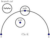
Figure 1: A smooth contour $C[a,b]$ in complex plane staring from $a$ to $b$. The blue dots and wave line denote the poles and branch cut of function $f(z)$ separately.

$$\int_{C[a,b]}f(z)dz=P\int_{a}^{b}f(z)dz+\sum n_{i}\oint_{C_{i}}f(z)dz.$$ (3)

Where the $C_{i}$ is a closed curve circling the pole or branch cut. The $P\int_{a}^{b}f(z)dz$ takes value in main single-valued branch. The winding number $n_{i}\in Z$ is the contour circling $n_{i}$ times around the pole or branch cut. In our previous work [15], we recalculated the axial (ABJ) anomaly [16, 17] by the formulae (3). We found the divergence of the axial current which is

$$q^{\rho}M_{5}^{\rho\mu\nu} = \frac{m^{2}}{2\pi^{2}}\epsilon^{\mu\nu}_{\quad\rho\sigma}k_{1}^{\rho}k_{2}^{\sigma}[\frac{1}{q^{2}}P\int_{0}^{1}\frac{1}{x}\ln\frac{1}{1-x(1-x)\frac{q^{2}}{m^{2}}}dx+\frac{1}{q^{2}}2\pi ik\ln\frac{1+\sqrt{1-\frac{4m^{2}}{q^{2}}}}{1-\sqrt{1-\frac{4m^{2}}{q^{2}}}}+\frac{1}{q^{2}}(2\pi i)^{2}n]$$ (6)

$$- \frac{1}{4\pi^{2}}\epsilon^{\mu\nu}_{\quad\rho\sigma}k_{1}^{\rho}k_{2}^{\sigma}+\left(\begin{array}[]{c}\mu\leftrightarrow\nu\\ k_{1}\leftrightarrow k_{2}\\ \end{array}\right).$$

Where the $n$ and $k$ are $n\in Z$ and $k\in Z$. We used the extra term $\frac{m^{2}}{2\pi^{2}}\epsilon^{\mu\nu}_{\quad\rho\sigma}k_{1}^{\rho}k_{2}^{\sigma}[-\frac{4\pi^{2}}{q^{2}}n]$ in equation (6) to cancel the anomaly term $-\frac{1}{4\pi^{2}}\epsilon^{\mu\nu}_{\quad\rho\sigma}k_{1}^{\rho}k_{2}^{\sigma}$. This leaded to the anomaly free condition

$$\boldsymbol{q^{2}=8n\pi^{2}m^{2}=m_{P}^{2}(n)},\quad n\in N.$$ (7)

Where $m_{P}$ is the neutral pseudoscalar meson mass for a quantum number $n$. The single-valued branches of multi-valued function are related to the bound states.

The paper is organized as follows. In Section 2, we study the positronium ($e^{+}e^{-}$) systems in ${\rm{QED_{3}}}$ with two-component Dirac fermion. We end with the conclusions.

2 Positronium ($e^{+}e^{-}$) systems in ${\rm{QED_{3}}}$ with two-component Dirac fermion

In this section, we consider the ${\rm{QED_{3}}}$ with single two-component Dirac fermion. The Lagrangian density of the theory is given by

$$\mathcal{L}=-\frac{1}{4}F_{\mu\nu}F^{\mu\nu}+\bar{\psi}(i\partial\!\!\!/-eA\!\!\!/-m)\psi.$$

We use the Minkowski metric tensor $g^{\mu\nu}={\rm{diag(1,-1,-1)}}$. The Dirac gamma matrices are defined by $\gamma^{0}=\sigma_{3},\gamma^{1}=i\sigma_{1},\gamma^{2}=i\sigma_{2}$, where the $\sigma_{i}$’s are the Pauli matrices. The $2\times 2$ Dirac matrices satisfy the identities:

$$\gamma^{\mu}\gamma^{\nu}=g^{\mu\nu}\textbf{1}-i\epsilon^{\mu\nu\rho}\gamma_{\rho},$$ (8)

$${\rm{tr}}(\gamma^{\mu}\gamma^{\nu}\gamma^{\rho})=-2i\epsilon^{\mu\nu\rho},$$

where we define the totally antisymmetric tensor $\epsilon^{\mu\nu\rho}$ so that $\epsilon^{012}=1$. Different with the 3 + 1 dimensional theories, the trace of three gamma matrices in 2+1 dimensions produces the totally antisymmetric $\epsilon^{\mu\nu\rho}$ symbol. We define $i\Pi^{\mu\nu}(q)$ to be the sum of all 1-particle-irreducible (1PI) insertions into the photon propagator. The expression of $i\Pi_{\mu\nu}(q)$ for one-loop amplitude (Fig. 2) is

Figure 2: The photon propagator with a single fermion loop insertion.

$$i\Pi_{\mu\nu}(q)=(-ie)^{2}(-1)\int\frac{d^{3}k}{(2\pi)^{3}}{\rm{tr}}[\gamma_{\mu}\frac{i}{k\!\!\!/-m}\gamma_{\nu}\frac{i}{k\!\!\!/+q\!\!\!/-m}].$$

Using the same method as ${\rm{QED_{4}}}$[18, 19, 20], we obtain

$$\Pi_{\mu\nu}(q)=(g_{\mu\nu}-\frac{q_{\mu}q_{\nu}}{q^{2}})\Pi_{1}(q^{2})+im\epsilon_{\mu\nu\rho}q^{\rho}\Pi_{2}(q^{2}),$$ (9)

where the expression of $\Pi_{1}(q^{2})$ and $\Pi_{1}(q^{2})$ are

$$\Pi_{1}(q^{2}) = 4ie^{2}q^{2}\int_{0}^{1}dx\ x(1-x)\int\frac{d^{3}k}{(2\pi)^{3}}\frac{1}{(k^{2}-\Delta)^{2}},$$

$$\Pi_{2}(q^{2}) = -2ie^{2}\int_{0}^{1}dx\int\frac{d^{3}k}{(2\pi)^{3}}\frac{1}{(k^{2}-\Delta)^{2}}.$$

The $\Delta$ is defined as

$$\Delta=m^{2}-x(1-x)q^{2}.$$

We Wick-rotate and substitute the Euclidean variable $k^{0}_{E}=-ik^{0}$. This gives

$$\Pi_{1}(q^{2}) = -4e^{2}q^{2}\int_{0}^{1}dx\ x(1-x)\int\frac{d\Omega_{3}}{(2\pi)^{3}}\int_{0}^{\infty}dk_{E}\frac{k^{2}_{E}}{(k_{E}^{2}+\Delta)^{2}}$$

$$= -4e^{2}q^{2}\int_{0}^{1}dx\ x(1-x)\int\frac{d\Omega_{3}}{(2\pi)^{3}}\int_{0}^{\infty}dk_{E}[\frac{1}{2i\sqrt{\Delta}}(\frac{1}{k_{E}-i\sqrt{\Delta}}-\frac{1}{k_{E}+i\sqrt{\Delta}})-\frac{\Delta}{(k_{E}^{2}+\Delta)^{2}}].$$

There are two poles at $k_{E}=\pm i\sqrt{\Delta}$. According to the formulae (3), we obtain

$$\Pi_{1}(q^{2})=\frac{e^{2}m}{16\pi t}[4t+(4+t^{2})\log(\frac{2-t}{2+t})](1+4n),$$ (10)

where the $n$ is $n\in Z$ and $t^{2}$ is defined as $t^{2}=\frac{q^{2}}{m^{2}}$. The ${\rm{QED_{3}}}$ is ultraviolet finite [2, 21, 22], we don’t need a soliton contribution to calculate the positronium state (different with the ultraviolet divergent theories [13]). The $\Pi_{2}(q^{2})$ can be calculated with the same method, that is

$$\Pi_{2}(q^{2}) = -2ie^{2}\int_{0}^{1}dx\int\frac{d^{3}k}{(2\pi)^{3}}\frac{1}{(k^{2}-\Delta)^{2}}$$ (11)

$$= \frac{e^{2}}{4\pi mt}\log(\frac{2+t}{2-t})(1+4k),$$

where the $k$ is $k\in Z$.

With the chain approximation (Figure 3), the photon propagator $G_{\mu\nu}(q)$ is then given by

$$G_{\mu\nu}(q) = \frac{-ig_{\mu\nu}}{q^{2}}+(\frac{-i}{q^{2}})i\Pi_{\mu\nu}(q)(\frac{-i}{q^{2}})+(\frac{-i}{q^{2}})i\Pi_{\mu}^{\eta}(q)(\frac{-i}{q^{2}})i\Pi_{\eta\nu}(q)(\frac{-i}{q^{2}})+\ldots$$

$$= \frac{-ig_{\mu\nu}}{q^{2}}+\frac{1}{q^{2}}\Pi_{\mu\eta}(q)G_{\nu}^{\eta}(q).$$

The dots indicate the iteration of the vacuum polarization tensor.

Figure 3: The photon propagator by the chain approximation.

From this expression, we find the $G_{\mu\nu}(q)$ satisfy the equation

$$(q^{2}g_{\mu\eta}-\Pi_{\mu\eta}(q))G_{\nu}^{\eta}(q)=-ig_{\mu\nu}.$$

After replacing $\Pi_{\mu\eta}(q)$ with the expression (9), we obtain

$$[q^{2}g_{\mu\eta}-(g_{\mu\eta}-\frac{q_{\mu}q_{\eta}}{q^{2}})\Pi_{1}(q^{2})-im\epsilon_{\mu\eta\rho}q^{\rho}\Pi_{2}(q^{2})]G_{\nu}^{\eta}(q)=-ig_{\mu\nu}.$$ (12)

To solve the $G_{\mu\nu}(q)$, we suppose that the $G_{\mu\nu}(q)$ is

$$G_{\mu\nu}(q)=g_{\mu\nu}\widetilde{\Pi}_{1}(q^{2})-\frac{q_{\mu}q_{\nu}}{q^{2}}\widetilde{\Pi}_{2}(q^{2})+im\epsilon_{\mu\nu\rho}q^{\rho}\widetilde{\Pi}_{3}(q^{2}),$$

where the $\widetilde{\Pi}_{1}(q^{2})$, $\widetilde{\Pi}_{2}(q^{2})$ and $\widetilde{\Pi}_{3}(q^{2})$ are unknown functions. Then the equation (12) becomes

$$g_{\mu\nu}[q^{2}-\Pi_{1}(q^{2})]\widetilde{\Pi}_{1}(q^{2})-q_{\mu}q_{\nu}[\widetilde{\Pi}_{2}(q^{2}) - \frac{\Pi_{1}(q^{2})\widetilde{\Pi}_{1}(q^{2})}{q^{2}}]-im\epsilon_{\mu\nu\rho}q^{\rho}[\Pi_{2}(q^{2})\widetilde{\Pi}_{1}(q^{2})-q^{2}\widetilde{\Pi}_{3}(q^{2})+\Pi_{1}(q^{2})\widetilde{\Pi}_{3}(q^{2})]$$ (13)

$$+ m^{2}\epsilon_{\mu\eta\rho}q^{\rho}\epsilon^{\eta}_{\nu\lambda}q^{\lambda}\Pi_{2}(q^{2})\widetilde{\Pi}_{3}(q^{2})=-ig_{\mu\nu}.$$

Where the $\epsilon_{\mu\eta\rho}q^{\rho}\epsilon^{\eta}_{\nu\lambda}q^{\lambda}$ can be calculated as

$$\epsilon_{\mu\eta\rho}q^{\rho}\epsilon^{\eta}_{\nu\lambda}q^{\lambda}=-g_{\mu\nu}q^{2}+q_{\mu}q_{\nu}.$$ (14)

From the equation (13), we obtain the $\widetilde{\Pi}_{1}(q^{2})$, $\widetilde{\Pi}_{2}(q^{2})$ and $\widetilde{\Pi}_{3}(q^{2})$ satisfy the equations

$$\begin{cases}[q^{2}-\Pi_{1}(q^{2})]\widetilde{\Pi}_{1}(q^{2})-m^{2}q^{2}\Pi_{2}(q^{2})\widetilde{\Pi}_{3}(q^{2})=-i,\\ \widetilde{\Pi}_{2}(q^{2})-\frac{\Pi_{1}(q^{2})\widetilde{\Pi}_{1}(q^{2})}{q^{2}}-m^{2}\Pi_{2}(q^{2})\widetilde{\Pi}_{3}(q^{2})=0,\\ \Pi_{2}(q^{2})\widetilde{\Pi}_{1}(q^{2})-q^{2}\widetilde{\Pi}_{3}(q^{2})+\Pi_{1}(q^{2})\widetilde{\Pi}_{3}(q^{2})=0.\end{cases}$$

The $\widetilde{\Pi}_{1}(q^{2})$, $\widetilde{\Pi}_{2}(q^{2})$ and $\widetilde{\Pi}_{3}(q^{2})$ can be solved as

$$\begin{cases}\widetilde{\Pi}_{1}(q^{2})=\frac{-i[q^{2}-\Pi_{1}(q^{2})]}{[q^{2}-\Pi_{1}(q^{2})]^{2}-m^{2}q^{2}[\Pi_{2}(q^{2})]^{2}},\\ \widetilde{\Pi}_{3}(q^{2})=\frac{-i\Pi_{2}(q^{2})}{[q^{2}-\Pi_{1}(q^{2})]^{2}-m^{2}q^{2}[\Pi_{2}(q^{2})]^{2}},\\ \widetilde{\Pi}_{2}(q^{2})=\frac{\Pi_{1}(q^{2})\widetilde{\Pi}_{1}(q^{2})}{q^{2}}+m^{2}\Pi_{2}(q^{2})\widetilde{\Pi}_{3}(q^{2}).\end{cases}$$

Then the pole of photon propagator $G_{\mu\nu}(q)$ is

$$[q^{2}-\Pi_{1}(q^{2})]^{2}-m^{2}q^{2}[\Pi_{2}(q^{2})]^{2}=0.$$ (15)

The energy eigenvalues of the bound states are the solutions of the equation (15). Using the expression of $\Pi_{1}(q^{2})$ (10) and $\Pi_{2}(q^{2})$ (11), the equation (15) can be rewritten as

$$\boxed{[m^{2}t^{2}-\frac{e^{2}m}{16\pi t}(4t+(4+t^{2})\log(\frac{2-t}{2+t}))(1+4n)]^{2}-[\frac{e^{2}m}{4\pi}\log(\frac{2+t}{2-t})(1+4n)]^{2}=0}.$$ (16)

Where the $m$ is the bare fermion mass. For simplify our discussion, we omit the unit of $m$ and $e^{2}$, where the $m$ and $e^{2}$ have the dimensions of ${\rm{(mass)}}$. Taking $e^{2}=0.5$ and $m=1$ for example, the solution of the bound state mass $M(e^{2},m,n)$, where $M(e^{2},m,n)$ is $M(e^{2},m,n)=\sqrt{q^{2}}=\sqrt{t^{2}m^{2}}$, can be obtained (Table 2 and Figure 4). The $M(0.5,1,n)$ have the behaviour $M(0.5,1,n)\sim a\log[b(n+\frac{1}{2})]$ which is the same as the WKB approximation results [23]. We also present the Figures of $M(0.25,m,n)$ and $M(e^{2},1,n)$ in Figure 5 and Figure 6 separately.

$n$	0	1	2	3	4	5	6
$M$	0.039	0.187	0.322	0.447	0.564	0.673	0.775
$n$	7	8	9	10	11	12	13
$M$	0.872	0.964	1.050	1.133	1.212	1.286	1.358

Table 2: Bound state masses $M(0.5,1,n)$

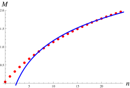
Figure 4: Bound state masses $M(0.5,1,n)$. Blue curve is the function $0.9\log[0.35(n+\frac{1}{2})]$.

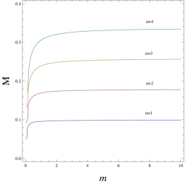
Figure 5: Bound state masses $M(0.25,m,n)$.

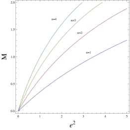
Figure 6: Bound state masses $M(e^{2},1,n)$.

To illustrate our results, we study the physical mass $m_{ph}$ of electron. The electron two-point function can be written as (Figure. 7)

Figure 7: The full electron propagator.

$$iG(p\!\!\!/) = \frac{i}{p\!\!\!/-m}+\frac{i}{p\!\!\!/-m}(i\Sigma(p\!\!\!/))\frac{i}{p\!\!\!/-m}+\cdots$$

$$= \frac{i}{p\!\!\!/-m+\Sigma(p\!\!\!/)}.$$

The $i\Sigma(p\!\!\!/)$ denote the sum of all one-particle irreducible (1PI) diagrams. The leading order term $i\Sigma_{2}(p\!\!\!/)$ is (Figure. 8)

Figure 8: the electron self-energy .

$$i\Sigma_{2}(p\!\!\!/) = (-ie)^{2}\int\frac{d^{3}k}{(2\pi)^{3}}\ \gamma^{\mu}\frac{i(k\!\!\!/+m)}{k^{2}-m^{2}+i\varepsilon}\gamma_{\mu}\frac{-i}{(k-p)^{2}+i\varepsilon}$$

$$= e^{2}\int_{0}^{1}dx\int\frac{d^{3}k}{(2\pi)^{3}}\frac{xp\!\!\!/-3m}{(k^{2}-\widetilde{\Delta}+i\varepsilon)^{2}}.$$

Where the $\widetilde{\Delta}$ is defined as $\widetilde{\Delta}=(1-x)(m^{2}-p^{2}x)$. According to the formulae (3), we obtain

$$i\Sigma_{2}(p\!\!\!/)=i\frac{e^{2}}{8\pi}\int_{0}^{1}dx\ \frac{xp\!\!\!/-3m}{\sqrt{\widetilde{\Delta}}}(1+4r),$$ (17)

where the $r$ is $r\in Z$. Then the physical mass $m_{ph}(e^{2},m,r)$ is the solution of the equation

$$\boxed{m_{ph}-m+\Sigma_{2}(m_{ph})=0}.$$ (18)

We should emphasize that the $i\Sigma_{2}(p\!\!\!/)$ is free of infrared divergence in our choice of gauge. From the equation (18), a real number solution $m_{ph}(e^{2},m,r)\in(0,m)$ for some $r\in Z$ exists. Suppose $e^{2}=0.5$ and $m=1$, the solution of equation (18) is (Figure 9)

$$m_{ph}\approx\begin{cases}0.64\quad r=-1,\\ 0.19\quad r=-2.\end{cases}$$

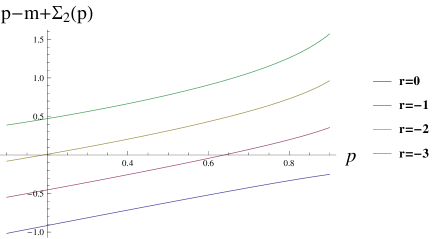
Figure 9: The curve of the function $p-m+\Sigma_{2}(p)$ with $m=1$, $e^{2}=0.5$ and $r$ ranging from $-3$ to $0$.

We find that the bound state masses $M(e^{2},m,n)$ have the excited states $M(e^{2},m,n)>2m_{ph}$ (Figure 4 or Table 2). This indicate that the ${\rm{QED_{3}}}$ have properties of confinement.

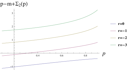
Figure 10: The curve of the function $p-m+\Sigma_{2}(p)$ with $m=1$, $e^{2}=1$ and $r$ ranging from $-3$ to $0$.

We now compare our results with the papers[8, 12] (Table 1). letting $e^{2}=1$ and $m=1$, the solution of the physical mass is $m_{ph}(1,1,-1)\approx 0.31082$ (Figure 10). We point out that the $m$ in equation (1) is the physical mass $m_{ph}$ instead of the bare fermion mass, that is

$$E_{n}^{l}=2m_{ph}+\frac{1}{4\pi}\ln m_{ph}+\frac{1}{2\pi}(\lambda_{n}^{l}-\frac{1}{2}\ln\frac{2}{\pi}).$$ (19)

The solution of the equation (16) have the properties that $M(1,1,n)>2m_{ph}(1,1,-1)$ at $n\geq 3$, then $M(1,1,n+3)$ correspond to $E_{n}^{l}$ in equation (19) with $n=0,1,2,3$. The results are put in Figure 11.

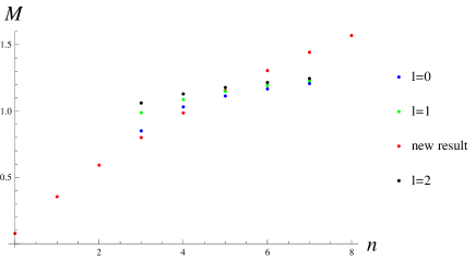
Figure 11: The red dots are our results. In here, we let $m=1$ and $e^{2}=1$. The other dots denote the results in Table 1. The total orbital angular momentum $l$ ranging from 0 to 2.

The vector positronium states correspond to the total angular momentum $J=1$ which have related to the total orbital angular momentum $L$ and the total spin $S$ as following

$$J=1\Leftrightarrow\begin{cases}L=0,S=1\\ L=1,S=0,1\\ L=2,S=1\end{cases}$$

From the Figure 11, we see that the vector positronium states which are related to the virtual photons have the total orbital angular momentum $L=0$. Then we put our results and the orbital angular momentum $l=0$ solutions of equation (19) in Table 3. From this we find that the first three values in our method are agreement with the ones in [8, 12]. To make the other two values consistent with each other, we need to calculate the higher order loops of $i\Pi^{\mu\nu}(q)$.

$n$	$0$	$1$	$2$	$3$	$4$
$M(1,1,n+3)$	0.8000	0.9858	1.1530	1.3047	1.4428
$E^{l=0}_{n}$	0.8506	1.0312	1.1133	1.1671	1.2072

Table 3: Comparing $M(1,1,n+3)$ with $E^{l=0}_{n}$.

3 Conclusions and Discussions

In this note, we have studied the positronium states in ${\rm{QED_{3}}}$. The results in the calculation of Feynman diagrams are the multi-value functions. Similar to our previous work [13, 15], these single-valued branches of multi-valued function are related to the bound states. we have calculated the photon propagator by the chain approximation and obtained the equation of energy eigenvalues of the vector positronium states. To illustrate the results, we also studied the electron physical mass in ${\rm{QED_{3}}}$. The real value electron physical mass $m_{ph}$ have been obtained by considering different single-valued branch of the multi-value function. Our results are agreement with the known ones in [8, 12].

References

[1]
J. M. Cornwall,
Phys. Rev. D 22 (1980), 1452
[2]
R. Jackiw and S. Templeton,
Phys. Rev. D 23 (1981), 2291
[3]
J. F. Schonfeld,
Nucl. Phys. B 185 (1981), 157-171
[4]
S. Deser, R. Jackiw and S. Templeton,
Annals Phys. 140 (1982), 372-411
[5]
C. J. Burden, J. Praschifka and C. D. Roberts,
Phys. Rev. D 46 (1992), 2695-2702
[6]
D. Sen,
Phys. Rev. D 41 (1990), 1227-1230
[7]
C. Yung and C. Hamer,
Phys. Rev. D 44 (1991), 2595-2597
[8]
A. Tam, C. Hamer and C. Yung,
J. Phys. G 21 (1995), 1463-1482
[9]
E. E. Salpeter and H. A. Bethe,
Phys. Rev. 84, 1232 (1951);
[10]
T. Allen and C. Burden,
Phys. Rev. D 53 (1996), 5842
[arXiv:hep-th/9512168 [hep-th]].
[11]
T. Allen and C. Burden,
Phys. Rev. D 55 (1997), 4954-4966
[arXiv:hep-th/9609150 [hep-th]].
[12]
V. G. Koures,
J. Comput. Phys. 128 (1996), 1
[arXiv:quant-ph/9510006 [quant-ph]].
[13]
C. Liu,
[arXiv:1811.06457 [hep-th]].
[14]
G. Källén,
Helv. Phys. Acta 25 (1952) no.4, 417;
H. Lehmann,
Nuovo Cim. 11 (1954), 342-357
[15]
Chang-Yong Liu,
“Note on anomalies in field theories,”
[ChinaXiv:202008.00076].
[16]
S. L. Adler,
Phys. Rev. 177 (1969), 2426-2438
doi:10.1103/PhysRev.177.2426
[17]
J. S. Bell and R. Jackiw,
Nuovo Cim. A 60 (1969), 47-61
doi:10.1007/BF02823296
[18]
W. Pauli and F. Villars,
Rev. Mod. Phys. 21, 434 (1949).
[19]
J. S. Schwinger,
Phys. Rev. 82, 664 (1951);
[20]
M. E. Peskin and D. V. Schroeder,
“An Introduction to quantum field theory,”
[21]
D. Cima, O.M., D. Franco and O. Piguet,
Phys. Rev. D 89 (2014) no.6, 065001
[22]
D. Cima, O.M.,
Phys. Lett. B 750 (2015), 1-5
[23]
M. I. Dobroliubov, D. Eliezer, I. I. Kogan, G. W. Semenoff and R. J. Szabo,
Mod. Phys. Lett. A 8 (1993), 2177-2188
[arXiv:hep-th/9302129 [hep-th]].