Switss: Computing Small
Witnessing Subsystems

Abstract

Witnessing subsystems for probabilistic reachability thresholds in discrete Markovian models are an important concept both as diagnostic information on why a property holds, and as input to refinement algorithms. We present Switss, a tool for the computation of Small WITnessing SubSystems. Switss implements exact and heuristic approaches based on reducing the problem to (mixed integer) linear programming. Returned subsystems can automatically be rendered graphically and are accompanied with a certificate which proves that the subsystem is indeed a witness.

I Introduction

A standard notion of a witness for a property in probabilistic systems is that of a subsystem [15, 17, 6, 1, 27, 26]. This is a part of the system that by itself already reaches a given probability threshold and thus serves as an explanation of why or where the property holds. Subsystems can also be used as input to automated refinement and synthesis algorithms. In [14] a counterexample guided abstraction refinement (CEGAR) method for probabilistic models is presented that iteratively refines a predicate abstraction by analyzing counterexamples (which are witnessing subsystems to the negated property). An application of small witnessing subsystems to synthesis is described in [8], where they are used to infer properties of a family of Markov chains from (a subsystem of) one of its members.

The aforementioned applications heavily benefit from witnessing subsystems that are small in terms of their state space. This paper presents Switss, a novel tool for the computation of small witnessing subsystems for reachability properties in Markovian models. Following [11], Switss proceeds by reduction to finding points of a polyhedron containing a large number of zero entries. These points also serve as certificates [22] for the fact that the computed subsystem indeed constitutes a witness.

We tackle the above problem from discrete geometry heuristically with an iterative linear programming (LP) approach. By adding binary variables to the LP, thus resulting in a mixed integer linear program (MILP), Switss can also compute minimal witnessing subsystems. In many applications, however, minimizing merely the state space of witnessing subsystems is insufficient in that it ignores the underlying structure of the model. For this reason, Switss supports label-based minimization, where syntactic units of the system can be subsumed under common labels.

Transparency and reliability are important factors for the evaluation of modern model checking software. Switss comes with a toolkit for the automated visualization of Markovian models and subsystems therein. For the convenience of (third-party) users, the framework includes a separate module for the independent verification of the associated certificates. In this way, results can be checked both visually and mathematically.

The translation to discrete geometry paired with the high level of encapsulation in our implementation makes Switss easily extendable. New heuristic approaches for finding vertices with many zeros (like vertex enumeration techniques) as well as different LP and MILP solvers used as backend engines can be integrated flexibly into Switss.

Comparison with related tools.

There are, to the best of our knowledge, three existing tools for the computation of witnessing subsystems: Dipro [3], Comics [16], and ltlsubsys [27]. We now compare each of these to Switss. A foreword that applies to all of them is that for Markov decision process (MDP), they only compute witnessing subsystems for lower bounds on maximal reachability probabilities. We emphasize that lower bounds on minimal reachability probabilities cannot be reduced to this case, but only to upper bounds on maximal reachability probabilities.

Dipro implements several heuristics for the computation of probabilistic counterexamples, only one of which directly operates on subsystems. This heuristic called XBF is available only for discrete-time Markov chains (DTMC), however. The other heuristics gather individual paths satisfying criteria like high probability mass or short length until the threshold is met. The subsystem resulting from these paths is not optimized along our state-minimality criterion (rather, the number of paths is minimized), so a comparison is problematic.

Comics implements heuristics for computing small subsystems in DTMCs, which are significantly different from the ones implemented in Switss. They rely on iteratively adding “probable” paths to the subsystem until the threshold is met. To compute the next such path, Comics uses graph algorithms. As each iteration requires computing the probability that has already been gathered, this approach often suffers from a substantial increase in time and memory consumption for growing thresholds, in contrast to our approach. With a prototypical implementation of what has now become Switss, we found that either our minimal or maximal reachability formulation (both of which are available for DTMCs) usually outperforms both Comics modes [11].

ltlsubsys [27] is the only tool for the computation of minimal witnesses in MDPs (it is, however, not publicly available). This tool also reduces the task of computing witnessing subsystems for maximal probabilities to a MILP which is related to our MILP formulations (cf. [11, Remark 6.2]). Its results in terms of upper and lower bounds on the number of states in a minimal witness found when hitting the timeout (which usually happens for bigger models) are comparable to ours [11]. As mentioned above, ltlsubsys cannot handle minimal reachability probabilities.

Summarizing the functionality, Switss is the first tool that implements (1) both exact and heuristic algorithms, with support for (2) both DTMCs and, more generally, MDPs, for (3) thresholds on both minimal and maximal reachability probabilities.

II Theoretical background

TABLE I: Overview of Farkas certificates for reachability properties in MDPs, where $\triangleleft\;\in\{\leq,<\}$ and $\triangleright\;\in\{\geq,>\}$.

Property	Source	Condition
$\mathbf{Pr}^{\min}_{s_{0}}(\lozenge{\text{\small goal}})\triangleright\lambda$	$\mathbf{z}\in\mathbb{R}^{S}$	$\mathbf{A}\mathbf{z}\leq\mathbf{b}\land\mathbf{z}(s_{0})\triangleright\lambda$
$\mathbf{Pr}^{\max}_{s_{0}}(\lozenge{\text{\small goal}})\triangleright\lambda$	$\mathbf{y}\in\mathbb{R}^{\mathcal{M}}_{\geq 0}$	$\mathbf{y}\mathbf{A}\leq\delta_{s_{0}}\land\mathbf{y}\mathbf{b}\triangleright\lambda$
$\mathbf{Pr}^{\min}_{s_{0}}(\lozenge{\text{\small goal}})\triangleleft\lambda$	$\mathbf{y}\in\mathbb{R}^{\mathcal{M}}_{\geq 0}$	$\mathbf{y}\mathbf{A}\geq\delta_{s_{0}}\land\mathbf{y}\mathbf{b}\triangleleft\lambda$
$\mathbf{Pr}^{\max}_{s_{0}}(\lozenge{\text{\small goal}})\triangleleft\lambda$	$\mathbf{z}\in\mathbb{R}^{S}$	$\mathbf{A}\mathbf{z}\geq\mathbf{b}\land\mathbf{z}(s_{0})\triangleleft\lambda$

A Markov decision process (MDP) is a tuple $\mathcal{M}=(S_{\operatorname{all}},\operatorname{Act},\mathbf{P},s_{0})$, where $S_{\operatorname{all}}$ is a finite set of states, $\operatorname{Act}$ is a finite set of actions, $\mathbf{P}\colon S_{\operatorname{all}}\times\operatorname{Act}\times S_{\operatorname{all}}\to[0,1]$ is the transition probability function where we require $\sum_{s^{\prime}\in S_{\operatorname{all}}}\mathbf{P}(s,\alpha,s^{\prime})\in\{0,1\}$ for all $(s,\alpha)\in S_{\operatorname{all}}\times\operatorname{Act}$, and $s_{0}$ is the initial state of $M$. We assume that there are two distinguished absorbing states $\operatorname{fail},\operatorname{goal}\in S_{\operatorname{all}}$, representing desirable and undesirable outcomes of the system. We will henceforth use the notation $S=S_{\operatorname{all}}\setminus\{\operatorname{fail},\operatorname{goal}\}$. We let $\operatorname{Act}(s)$ be the set of actions satisfying $\sum_{s^{\prime}\in S_{\operatorname{all}}}\mathbf{P}(s,\alpha,s^{\prime})=1$. We require $\operatorname{Act}(s)\neq\varnothing$ for all $s\in S$ and sometimes write $\mathcal{M}=\{(s,\alpha)\mid s\in S,\,\alpha\in\operatorname{Act}(s)\}$.

The system begins in $s_{0}$ and evolves as follows: in state $s$, an action $\alpha\in\operatorname{Act}(s)$ is chosen non-deterministically and the next state is picked according to the distribution $\mathbf{P}(s,\alpha,\cdot)$. A scheduler $\mathfrak{S}$ is some resolution of the non-determinism and induces a probability $\mathrm{Pr}^{\mathfrak{S}}_{\mathcal{M},s_{0}}(\lozenge\operatorname{goal})$ to eventually reach $\operatorname{goal}$ (see [5, Section 10.6]). We are interested in the minimal and maximal reachability probabilities attained among all schedulers, denoted by $\mathbf{Pr}^{\min}_{\mathcal{M},s_{0}}(\lozenge\operatorname{goal})$ and $\mathbf{Pr}^{\max}_{\mathcal{M},s_{0}}(\lozenge\operatorname{goal})$. They represent worst- and best-case scenarios for the behavior of the system.

A subsystem of $\mathcal{M}$ is an MDP obtained from $\mathcal{M}$ by deleting states from $S$ and redirecting transitions to $\operatorname{fail}$. If $\mathcal{M}$ satisfies $\mathbf{Pr}^{*}_{\mathcal{M},s_{0}}(\lozenge\operatorname{goal})\geq\lambda$ for $*\in\{\min,\max\}$, one way of analyzing which parts of the system are sufficient for this inequality is to find a subsystem $\mathcal{M}^{\prime}$ of $\mathcal{M}$ already satisfying the lower bound, i.e., $\mathbf{Pr}^{*}_{\mathcal{M}^{\prime},s_{0}}(\lozenge\operatorname{goal})\geq\lambda$. We call these witnessing subsystems. We aim at finding small (or minimal) witnessing subsystems in terms of how many states they include.

In [11] we proposed a translation between witnessing subsystems and Farkas certificates (which are vectors satisfying the conditions in Table I) for lower-bounded reachability thresholds. Here, $\mathbf{A}\in\mathbb{R}^{\mathcal{M}\times S}$ and $\mathbf{b}\in\mathbb{R}^{S}$ are defined as follows: $\mathbf{A}((s,\alpha),t)=1-\mathbf{P}(s,\alpha,s)$ if $s=t$ and $-\mathbf{P}(s,\alpha,t)$ otherwise, and $\mathbf{b}(s,\alpha)=\mathbf{P}(s,\alpha,\operatorname{goal})$.

In this paper, we are mainly interested in the first two rows of Table I with $\triangleright=\,\geq$, and denote the corresponding sets of Farkas certificates by $\mathcal{P}^{\min}_{\mathcal{M}}(\lambda)\subseteq\mathbb{R}^{S}_{\geq 0}$ and $\mathcal{P}^{\max}_{\mathcal{M}}(\lambda)\subseteq\mathbb{R}^{\mathcal{M}}_{\geq 0}$. The passage from a Farkas certificate $\mathbf{z}\in\mathcal{P}^{\min}_{\mathcal{M}}(\lambda)$ (resp. $\mathbf{y}\in\mathcal{P}^{\max}_{\mathcal{M}}(\lambda)$) to a subsystem of $\mathcal{M}$ works by including all states with $\mathbf{z}(s)>0$ (resp. $\mathbf{y}(s,\alpha)>0$ for some $\alpha$), and all edges between such states. All other edges are redirected to $\operatorname{fail}$. Thus, computing minimal (small) witnessing subsystems for $\mathbf{Pr}^{*}_{\mathcal{M},s_{0}}(\lozenge\operatorname{goal})\geq\lambda$ can be reduced to finding points in $\mathcal{P}^{*}_{\mathcal{M}}(\lambda)$ with a maximal (large) number of zeros.

As in [11] we have to assume that the only maximal end components of $\mathcal{M}$ are $\{\operatorname{goal}\}$ and $\{\operatorname{fail}\}$. This means that almost all paths reach either of these two states under every scheduler. This can be ensured by a preprocessing step whose time-complexity is at most quadratic in the underlying graph, see [9, 2].

III Implementation and features

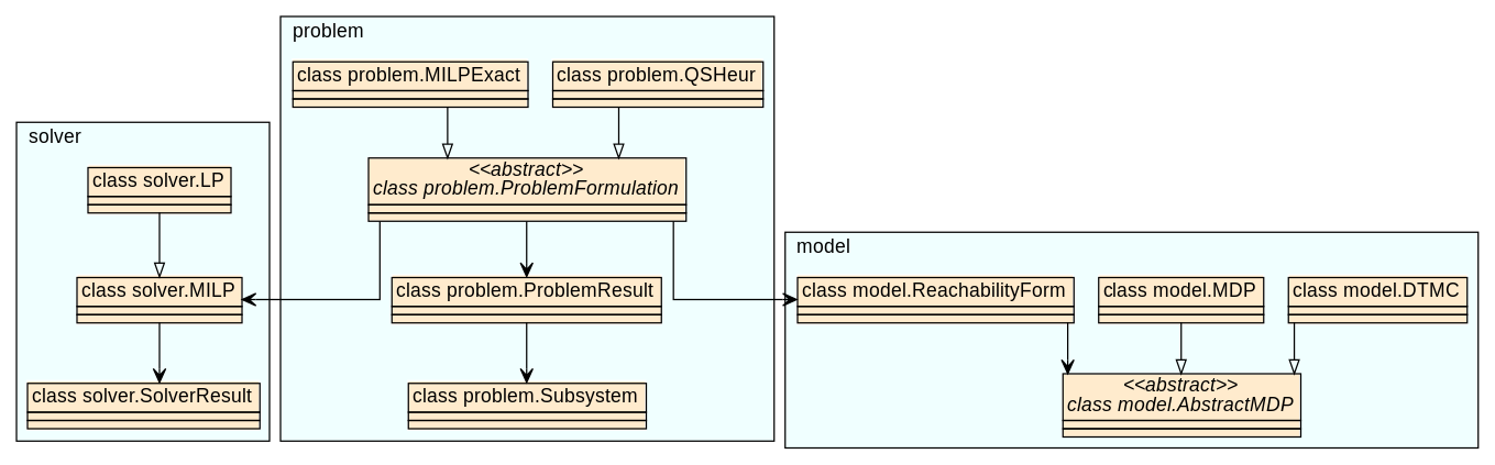
Figure 1: Switss contains modules for modeling DTMCs and MDPs (switss.model), different approaches to finding small (or minimal) subsystems (switss.problem) and interfaces to MILP and LP solvers, built on top of the PuLP library (switss.solver). The model.ReachabilityForm class is a wrapper for DTMCs/MDPs which fulfill the requirements as given in Section II (having a single target and fail state, etc.). Finding small subsystems is done through implementations of problem.ProblemFormulation, e.g. by using the quotient sum heuristics (problem.QSHeur) or the MILP formulation (problem.MILPExact). Additionally included are modules for benchmarking (switss.benchmarks), generating and verifying Farkas certificates (switss.certfication) and interaction with Prism and Prism file formats (switss.prism).

Switss is a complete re-implementation and substantial extension of the prototype implementation that was used to run the experiments presented in [11]. An overview of the structure of Switss is given in Figure 1. Apart from increased usability and an extensive documentation and testing suite, the main extensions are the following:

• Functions to generate and verify certificates for all senses ($\leq,<,\geq,>$) and modes (min/max).

• Visualization of MDP subsystems.

• A generalized notion of minimality that allows to minimize “active labels” [25] in the subsystem (both exactly and heuristically).

• New heuristics for the computation of witnessing subsystems with few states.

• Support for various LP/MILP solvers.

Switss is implemented in python and can be included as a library, or used as a stand-alone tool. MDPs and DTMCs can be loaded either from the explicit transition matrix format (.tra), or from a model specified in the Prism [19] guarded command language. In the latter case, Switss uses Prism to derive an explicit transition matrix representation. The library PuLP is used as modeling language for linear programs, and as an interface to various LP/MILP solvers, where we currently support: Gurobi [12], Cplex, Cbc and Glpk. While the first two are proprietary software (both offer academic licenses), the latter two are open source.

III-A Computing and verifying Farkas certificates

Generating Farkas certificates (for a specified threshold, sense and mode) amounts to finding a vector satisfying the corresponding linear inequalities as presented in Table I. For the non-strict inequalities, this can be done directly by solving an LP, where the objective function can be arbitrary. Handling strict inequalities can be done by replacing the strict inequality by its non-strict counterpart, and then optimizing in the direction where strict inequality is required. A Farkas certificate exists if and only if the solution satisfies the strict inequality (and the solution is then a certificate).

To verify that a given vector $\mathbf{v}$ is a Farkas certificate, it is enough to check that it satisfies the inequalities. Due to the varying precision of solvers and the python numerical libraries, it can happen that exact satisfaction of the certificate condition is not given. Hence we allow a tolerance $t$ to be passed as an option to the certificate verifier, which will then check, for example, that:

$$\mathbf{A}\mathbf{v}-\mathbf{t}\leq\mathbf{b}\land\mathbf{v}(s_{0})+t\geq\lambda$$

where $\mathbf{t}$ is the vector of appropriate dimension containing $t$ in every entry. In the future, we plan to explore how robust certificates (which can be verified with $t=0$) can be generated efficiently and consistently (e.g. by searching for vectors that do not lie on the boundary of the polytope).

III-B New heuristics

To find points in $\mathcal{P}^{*}_{\mathcal{M}}(\lambda)$ with many zeros, the quotient-sum (QS) heuristic [11] iteratively solves LPs over the polytope $\mathcal{P}^{*}_{\mathcal{M}}(\lambda)$. The objective function is updated in every step in a way that aims at pushing as many entries of the solutions vectors to zero as possible. The LP that is solved for $\mathcal{P}_{\mathcal{M}}^{\min}(\lambda)$ is:

$$\min\sum_{s\in S}\mathbf{o}_{i}(s)\mathbf{z}(s)\;\;\text{ s.t. }\quad\mathbf{z}\in\mathcal{P}^{\min}_{\mathcal{M}}(\lambda)$$ (III.1)

We put $\mathbf{o}_{0}=(1,\ldots,1)\in\mathbb{R}^{S}$ and compute $\mathbf{o}_{j+1}$ from a solution $\mathbf{z}_{j}$ of the $j$-th iteration by the quotient rule: $\mathbf{o}_{j+1}(s)=1/\mathbf{z}_{j}(s)$ if $\mathbf{z}_{j}(s)>0$, and else $\mathbf{o}_{j+1}(s)=C$ for some big $C$. Hence, a dimension close to zero will have a high “cost” in the next iteration.

While the heuristics generally yield small subsystems fast (especially when compared with the time it takes to exactly minimize the number of states with a MILP), sometimes “spikes” were observed: the heuristics returned a worse result when decreasing $\lambda$. As a witnessing subsystem for $\lambda$ is also witnessing for all $\lambda^{\prime}\leq\lambda$, this is undesirable.

In Switss both the initial objective $\mathbf{o}_{0}$ and the update can be customized. As shown by our experiments (Section V), the choice of $\mathbf{o}_{0}$ may have a substantial effect on the performance of the heuristics (first experiments on changing the update did not lead to better performance). We propose the following candidate values for $\mathbf{o}_{0}$. For the heuristic related to $\mathbf{Pr}^{\max}$, we take $\mathbf{o}_{0}$ to be the inverse of a solution to the following LP (where the inverse is the result of pointwise $1/\cdot$, if the corresponding entry is greater 0, and a big constant otherwise):

$$\max\,\mathbf{y}\mathbf{b}\;\;\text{\footnotesize s.t. }\;\;\mathbf{y}\in\mathcal{P}^{\max}_{\mathcal{M}}(0)$$ (III.2)

For $\mathbf{Pr}^{\min}$ we let $\mathbf{o}_{0}$ be the inverse of a solution to:

$$\max\sum_{s\in S}\mathbf{z}(s)\;\;\text{\footnotesize s.t. }\;\;\mathbf{z}\in\mathcal{P}^{\min}_{\mathcal{M}}(0)$$ (III.3)

Putting $\lambda=0$ discards the constraint $\mathbf{z}(s_{0})\geq\lambda$ for $*=\min$ and $\mathbf{y}\mathbf{b}\geq\lambda$ for $*=\max$ (compare Table I). If $\mathcal{M}$ is a DTMC, then a solution vector of Equation III.2 contains the expected number of visits to a state and a solution of Equation III.3 contains the probability to reach $\operatorname{goal}$ from every state. Intuitively, states with a low entry in these vectors contribute less to the probability of reaching $\operatorname{goal}$ from the initial state, and hence should get a higher value in $\mathbf{o}_{0}$. Similar importance measures where considered in the context of counterexample generation in [7].

III-C Label-based minimization

The idea of minimizing not the number of states, but the number of labels present in a subsystem was first considered in [25]. There it was used to minimize the number of “active” commands for MDPs given in Prism language. We have extended the approach of [11] to allow label-based minimization in a similar way as was done in [25]. This allows applying the QS-heuristic to the computation of subsystems with few active labels. Further interesting use cases could be minimizing participating components (for compositional systems) in a witnessing subsystem, or the number of controllable states.

Our extension works as follows. Take an MDP $\mathcal{M}$ with states $S\cup\{\operatorname{goal},\operatorname{fail}\}$ a finite set of labels $L$ and $\Lambda:S\to 2^{L}$. Now let $\sigma$ be a vector with $|L|$ variables with domain $[0,1]$ and consider the following LPs, which generalize the LPs of [11, Section 6]:

$$\min\sum_{l\in L}\sigma(l)\text{ \footnotesize s.t.}\;\;\;\stackanchor{\mathbf{z}\in\mathcal{P}^{\min}_{\mathcal{M}}(\lambda)\;\;}{\mathbf{z}(s)\leq\sigma(l)\,\;\;\;\text{ \footnotesize f.a. }\;\,{\begin{subarray}{c}s\in S\\ l\in\Lambda(s)\end{subarray}}}$$ (III.4)

$$\min\sum_{l\in L}\sigma(l)\text{ \footnotesize s.t.}\;\stackanchor{\mathbf{y}\in\mathcal{P}^{\max}_{\mathcal{M}}(\lambda)\;\,\;\;\;\;\,}{\mathbf{y}(s,\alpha)\leq K\cdot\sigma(l)\,\text{ \footnotesize f.a. }{\begin{subarray}{c}(s,\alpha)\in\mathcal{M}\\ l\in\Lambda(s)\end{subarray}}}$$ (III.5)

The factor $K$ in Equation III.5 is an upper bound on any entry of any vector $\mathbf{y}\in\mathcal{P}_{\mathcal{M}}^{\max}(\lambda)$ (here we use that $\mathcal{P}_{\mathcal{M}}^{*}(\lambda)$ is bounded, cf. [11, Lemma 5.1]). It can be computed by first maximizing the sum of all entries over all vectors in $\mathcal{P}_{\mathcal{M}}^{\max}(\lambda)$ using an LP, and taking the objective value of the solution to be $K$. The first LP does not need this step, as $1$ is an upper bound on all entries in any vector $\mathbf{z}\in\mathcal{P}_{\mathcal{M}}^{\min}(\lambda)$.

A solution $(\mathbf{z},\sigma)$ of Equation III.4 with $N$ non-zero entries in $\sigma$ can be translated into a witnessing subsystem for $\mathbf{Pr}^{\min}_{\mathcal{M}}(\lozenge\operatorname{goal})\geq\lambda$ with $N$ labels. Conversely, a witnessing subsystem with $N$ active labels induces a solution $(\mathbf{z},\sigma)$ such that $\sigma$ has $N$ non-zero entries. The same holds for Equation III.5.

The QS-heuristic can be adapted to label-based minimization by trying to push only the entries of $\sigma$ to zero. This algorithm is implemented in Switss. Restricting the domain of $\sigma$-variables in Equations III.4 and III.5 to $\{0,1\}$ yields a MILP, whose solutions correspond to witnessing subsystems with a minimal amount of present labels.

Figure 2: Visualization of a subsystem (which excludes the gray states) by Switss . The other colors indicate a user defined labeling. If the subsystem is induced by a Farkas certificate (e.g. as returned by the QS-heuristic) Switss prints the corresponding values in each state (or action, for “max”-queries).

IV A tour of Switss

The following tour can be reproduced using the supplementary material [18]. We first load an MDP:

In: mc = MDP.from_file(        "ex_mdp.lab", "ex_mdp.tra")The following command renders the MDP (we have rebuilt the MDP in tikz for a better presentation and refer to Figure 2 for an example output of Switss):

In: mc.digraph()

Out:

We first transform the MDP into so-called reachability form (RF), which can be thought of as a standardized format for reachability analysis. It can be constructed from a DTMC or MDP, an initial state (which should be unique), and a set of target states. The method reduce performs forward (from the intial state) and backward (from the target states) reachability queries and removes all states that are either unreachable, or do not reach $\operatorname{goal}$. A new distinguished target state is added, which receives an incoming edge from each original target state.

In: rf,_,_ = ReachabilityForm.reduce(        mc, "init", "goal")    rf.system.digraph()

Out:

IV-A Certification

Next we demonstrate how Farkas certificates can be generated (by generate_farkas_certificate) and verified (by check_farkas_certificate). These methods take an RF and a specification of the threshold property to be certified. We first generate a certificate using Cbc and verify its validity.

In: cert = generate_farkas_certificate(        rf, "max", ">=", 0.55, solver="cbc")

In: check_farkas_certificate(        rf, "max", ">=", 0.55, cert)

Out: True

If the threshold property is not satisfied by the model, no Farkas certificate can be produced.

In: fark_cert = generate_farkas_certificate(        rf, "min", ">=", 0.55, solver="cbc")

Out: Property is not satisfied!

IV-B Witnessing subsystems

We illustrate the computation of witnessing subsystems, beginning with the methods for exactly minimizing the number of states. In contrast to the certification module, we only consider lower-bounded thresholds here, as reachability probabilities cannot increase in subsystems.

IV-B1 Minimal witnessing subsystems

The class MILPExact (an instance of ProblemFormulation) is used to specify queries for exact minimization of an RF for a given threshold property. It is initialized by specifying mode (min or max) and solver:

In: milp_exact_max = MILPExact(        "max", solver="cbc")

The solve method now takes an RF and a threshold, constructs the MILP and solves it by calling the specified solver.

In: res = milp_exact_max.solve(rf, 0.1)

If successful, the result contains a subsystem that can also be rendered graphically, where pale states do not belong to the subsystem:

In: res.subsystem.digraph()

Out:

If the threshold is increased to $0.3$, the minimal witnessing subsystem uses the upper branch:

In: res = milp_exact_max.solve(rf, 0.3)

In: res.subsystem.digraph()

Out:

We now consider witnesses for minimal reachability. Such a witness needs to ensure that the threshold is met by all possible schedulers. For $0.1$, it is enough to include the upper branch and the first state in the lower branch, but for $0.3$ already all states have to be included.

In: milp_exact_min = MILPExact(        "min", solver="cbc")

In: res = milp_exact_min.solve(rf, 0.1)    res.subsystem.digraph()

Out:

IV-B2 The QS-heuristic

The counterpart of MILPExact for the heuristic computations of small (rather than minimal) witnessing subsystems is QSHeur. As it is an iterative heuristic, we can use the method solveiter to return an iterator over the results. In our example, all three iterations return the same subsystem, which is not optimal, however (compare with the results of the exact query for maximum probability and threshold $0.1$).

In: qs_max_heur = QSHeur(        "max", solver="cbc", iterations=3)    results = list(        qs_max_heur.solveiter(rf, 0.1))    print_results(results)

Out: -- results --subsys states:5, value: 5subsys states:5, value: 5subsys states:5, value: 5

In: results[2].subsystem.digraph()

Out:

The corresponding computation for minimum probabilities improves after the first iteration and returns the optimal witness (the default number of iterations of the heuristics is three).

In: qs_min_heur = QSHeur(        "min", solver="cbc")    results = list(        qs_min_heur.solveiter(rf, 0.1))    print_results(results)

Out: -- results --subsys states:7, value: 7subsys states:5, value: 5subsys states:5, value: 5

In: results[2].subsystem.digraph() Out:

IV-C Label-based minimization

Now suppose that we do not want to minimize the amount of states present in the subsystem, but the amount of colors that it includes. The colors stand for some labeling that may interest the user. That is, the lower branch counts as one, as it only includes one color, while the upper branch counts two although it has a state less. We specify this optimization objective by using the labels parameter of the solve method.

In: milp_exact_labels = MILPExact(        "max", solver="cbc")    result_labels = milp_exact_labels.solve(        rf, 0.3,labels=["blue","green","brown"])    print_result(result_labels)

Out: subsys states: 5, value: 1.0In contrast to minimizing the number of states, now taking the entire lower branch is optimal for maximal reachability probabilities and threshold $0.3$. The objective value of this subsystem is $1$, as it only includes one of the labels.

In: result_labels.subsystem.digraph()

Out:

V Experiments

We have run experiments on a number of models available in the benchmark suite of Prism. The results and all scripts used to produce them are included in the supplementary material [18]. We used a computer with two Intel Xeon L5630 CPUs at 2.13GHz with four cores each and 189GB of RAM. Each computation was assigned four cores, a memory limit of 10GB and each call to an LP/MILP solver (we use Gurobi, version 9.0.1) was limited to 20 minutes.

Figure 3: Comparison of subsystem sizes achieved by the heuristics of Switss for benchmark DTMCs.

We consider the following models, where the first two are DTMCs and the last two are MDPs: the bounded retransmission protocol [10, 13] (brp-N-K), the crowds protocol [24, 23] (crowds-N-K), the randomized consensus protocol [20, 4] (consensus-N-K) and the csma-N-K protocol for data channels [21]. In all cases increasing N and K, (which, for example, stand for the number of participating members, or a bound on possible random walks) leads to larger models. For each model we fixed a reachability objective, inspired by properties considered in the benchmark suite.

We contrast the results of the QS-heuristic with initial objective $(1,\ldots,1)$ (called AO for “all-ones”), and the initial objectives $\operatorname{InvF}{}$ and $\operatorname{InvP}{}$, which are inverses of solutions of Equations III.2 and III.3, respectively. As $\operatorname{InvF}{}$ is derived from the $\mathcal{P}^{\max}_{\mathcal{M}}(\lambda)$ polytope, we apply it to the max-queries, and conversely for $\operatorname{InvP}{}$. We let the QS-heuristic compute five iterations. The subscripts $i$ in AO_i, $\operatorname{InvF}{}_{i}$ and $\operatorname{InvP}{}_{i}$ refer to the result at iteration $i$. As the last iterations do not yield much improvement we only consider the first three iterations in Figure 3 and Figure 4. If no improvement was made after the $i$-th iteration, we do not show the following ones.

We examine for each model the time needed to compute the reachability form (from an explicit transition matrix) and the maximal time (over min/max-forms, all considered thresholds and initial values) needed to compute five iterations of the QS-heuristic, given the RF. This latter value is called max-time.

We first consider the DTMCs: crowds-5-8 (27,849 states, 11.3 $\mathrm{s}$ to construct RF, max-time: 191.6 $\mathrm{s}$) and brp-1024-2 (31,749 states, 9.4 $\mathrm{s}$ to construct RF, max-time: 366.1 $\mathrm{s}$). As $\mathbf{Pr}^{\max}_{\mathcal{M}}(\lozenge\operatorname{goal})=\mathbf{Pr}^{\min}_{\mathcal{M}}(\lozenge\operatorname{goal})$ if $\mathcal{M}$ is a DTMC, witnesses for max- and min-probabilities coincide. Still, the QS-heuristic applied to the polytopes $\mathcal{P}^{\max}_{\mathcal{M}}(\lambda)$, and $\mathcal{P}^{\min}_{\mathcal{M}}(\lambda)$ yields different results. This was already observed in [11], where it was also noted that one of the two usually performs well with the initial objective AO (the only one considered in [11]). The new experiments show that $\operatorname{InvF}{}$ and $\operatorname{InvP}{}$ are better initial vectors for the considered instances (see the difference between AO₃ and $\operatorname{InvF}_{1}$ in crowds-5-8 max and, respectively, $\operatorname{InvP}_{2}$ in brp-1024-2 min of Figure 3). The new heuristics also tend to stabilise after fewer iterations.

Figure 4: Comparison of subsystem sizes achieved by the heuristics of Switss for benchmark MDPs.

The MDPs that we consider are: consensus-2-6 (786 states, 1170 state-action pairs, 0.3 $\mathrm{s}$ to construct RF, max-time: 3.5 $\mathrm{s}$) and CSMA-2-6 (66,720 states, 66,790 state-action pairs, 18.5 $\mathrm{s}$ to construct RF, max-time: 512.7 $\mathrm{s}$). The new heuristics have a mixed effect here: in the max-case, CSMA-2-6 profits while for consensus-2-6 the AO-initialization yields better results. For min, AO and $\operatorname{InvP}$ perform equally well. It should be noted that in CSMA-2-6 the number of actions per state is very close to one, and hence it is “close” to being a DTMC. For consensus-2-6 it is noteworthy that relatively small subsystems are possible for maximal reachability throughout all considered thresholds.

The experiments show that the QS-heuristic is able to compute small witnessing subsystems in a reasonable time for models with over 60,000 states, and that the new heuristics perform well. As the exact computations via MILP run into the timeout for all of the models in Figure 3 and Figure 4, we cannot say how far the computed subsystems are from the optimal ones in terms of their size. However, generalizing from smaller instances (see Figure 5) indicates that the performance of the heuristic is good.

Figure 5: The QS-heuristic vs. exact minimization.

VI Conclusion

We have presented Switss, a tool for computing small witnessing subsystems in discrete Markovian models. Contrary to other tools in the field, Switss takes a unified approach for all scenarios that have been considered in the literature (minimal and maximal probabilities, exact and heuristic computation). New initial objective functions in the QS-heuristic have been shown to improve previous results for DTMCs. Our tool also comes with the complete functionality of a certificate generator and verifier for reachability problems in MDPs.

In future work we will investigate which properties of a DTMC benefit either the minimal or the maximal probability formulation, and add an automated detection scheme to Switss in order to avoid redundant computations. We also intend to incorporate a new class of heuristics based on vertex enumeration algorithms.

References

- [1] Ábrahám, E., Becker, B., Dehnert, C., Jansen, N., Katoen, J., Wimmer, R.: Counterexample generation for discrete-time Markov models: An introductory survey. In: 14th International School on Formal Methods for the Design of Computer, Communication, and Software Systems, SFM 2014. pp. 65–121 (2014), https://doi.org/10.1007/978-3-319-07317-0_3
- [2] de Alfaro, L.: Formal verification of probabilistic systems. Ph.D. thesis, Stanford University, Department of Computer Science (1997)
- [3] Aljazzar, H., Leitner-Fischer, F., Leue, S., Simeonov, D.: Dipro - A tool for probabilistic counterexample generation. In: Model Checking Software - 18th International SPIN Workshop 2011. pp. 183–187 (2011), https://doi.org/10.1007/978-3-642-22306-8_13
- [4] Aspnes, J., Herlihy, M.: Fast randomized consensus using shared memory. Journal of Algorithms 11(3), 441–461 (1990), https://doi.org/10.1016/0196-6774(90)90021-6
- [5] Baier, C., Katoen, J.P.: Principles of Model Checking (Representation and Mind Series). The MIT Press, Cambridge, MA (2008)
- [6] Braitling, B., Wimmer, R., Becker, B., Jansen, N., Ábrahám, E.: Counterexample generation for Markov chains using SMT-based bounded model checking. In: Formal Techniques for Distributed Systems - Joint 13th IFIP WG 6.1 International Conference, FMOODS 2011, and 31st IFIP WG 6.1 International Conference, FORTE 2011. pp. 75–89 (2011), https://doi.org/10.1007/978-3-642-21461-5_5
- [7] Brázdil, T., Chatterjee, K., Chmelik, M., Fellner, A., Kretínský, J.: Counterexample explanation by learning small strategies in Markov decision processes. In: Computer Aided Verification - 27th International Conference, CAV 2015 (2015), https://doi.org/10.1007/978-3-319-21690-4_10
- [8] Ceska, M., Hensel, C., Junges, S., Katoen, J.: Counterexample-driven synthesis for probabilistic program sketches. In: Formal Methods - The Next 30 Years - Third World Congress, FM 2019. pp. 101–120 (2019), https://doi.org/10.1007/978-3-030-30942-8_8
- [9] Chatterjee, K., Henzinger, M.: Faster and dynamic algorithms for maximal end-component decomposition and related graph problems in probabilistic verification. In: Proceedings of the Twenty-Second Annual ACM-SIAM Symposium on Discrete Algorithms, SODA (2011), https://doi.org/10.1137/1.9781611973082.101
- [10] D’Argenio, P.R., Jeannet, B., Jensen, H.E., Larsen, K.G.: Reachability analysis of probabilistic systems by successive refinements. In: Process Algebra and Probabilistic Methods, Performance Modeling and Verification: Joint International Workshop, PAPM-PROBMIV 2001. pp. 39–56 (2001), https://doi.org/10.1007/3-540-44804-7_3
- [11] Funke, F., Jantsch, S., Baier, C.: Farkas certificates and minimal witnesses for probabilistic reachability constraints. In: Biere, A., Parker, D. (eds.) Tools and Algorithms for the Construction and Analysis of Systems. pp. 324–345. Springer International Publishing, Cham (2020), https://doi.org/10.1007/978-3-030-45190-5_18
- [12] Gurobi Optimization LLC, L.: Gurobi optimizer reference manual (2020), http://www.gurobi.com
- [13] Helmink, L., Sellink, M.P.A., Vaandrager, F.W.: Proof-checking a data link protocol. In: Types for Proofs and Programs, International Workshop TYPES’93. pp. 127–165 (1993), https://doi.org/10.1007/3-540-58085-9_75
- [14] Hermanns, H., Wachter, B., Zhang, L.: Probabilistic CEGAR. In: Computer Aided Verification, 20th International Conference, CAV 2008. pp. 162–175 (2008), https://doi.org/10.1007/978-3-540-70545-1_16
- [15] Jansen, N., Ábrahám, E., Katelaan, J., Wimmer, R., Katoen, J., Becker, B.: Hierarchical counterexamples for discrete-time Markov chains. In: Automated Technology for Verification and Analysis, 9th International Symposium, ATVA 2011. pp. 443–452 (2011), https://doi.org/10.1007/978-3-642-24372-1_33
- [16] Jansen, N., Ábrahám, E., Volk, M., Wimmer, R., Katoen, J.P., Becker, B.: The COMICS Tool – Computing Minimal Counterexamples for DTMCs. In: Automated Technology for Verification and Analysis. pp. 349–353. Springer, Berlin, Heidelberg (2012), https://doi.org/10.1007/978-3-642-33386-6_27
- [17] Jansen, N., Wimmer, R., Ábrahám, E., Zajzon, B., Katoen, J., Becker, B., Schuster, J.: Symbolic counterexample generation for large discrete-time Markov chains. Science of Computer Programming 91, 90–114 (2014), https://doi.org/10.1016/j.scico.2014.02.001
- [18] Jantsch, S., Harder, H., Funke, F., Baier, C.: fmcad20-material.zip (2020), https://doi.org/10.6084/m9.figshare.12682253.v2
- [19] Kwiatkowska, M.Z., Norman, G., Parker, D.: PRISM 4.0: Verification of probabilistic real-time systems. In: Computer Aided Verification - 23rd International Conference, CAV 2011. pp. 585–591 (2011), https://doi.org/10.1007/978-3-642-22110-1_47
- [20] Kwiatkowska, M.Z., Norman, G., Segala, R.: Automated verification of a randomized distributed consensus protocol using cadence SMV and PRISM. In: Computer Aided Verification, 13th International Conference, CAV 2001. pp. 194–206 (2001), https://doi.org/10.1007/3-540-44585-4_17
- [21] Kwiatkowska, M.Z., Norman, G., Sproston, J., Wang, F.: Symbolic model checking for probabilistic timed automata. Information and Computation 205(7), 1027–1077 (2007), https://doi.org/10.1016/j.ic.2007.01.004
- [22] McConnell, R.M., Mehlhorn, K., Näher, S., Schweitzer, P.: Certifying algorithms. Computer Science Review 5(2), 119–161 (2011), https://doi.org/10.1016/j.cosrev.2010.09.009
- [23] Reiter, M.K., Rubin, A.D.: Crowds: Anonymity for web transactions. ACM Transactions on Information and System Security 1(1), 66–92 (1998), https://doi.org/10.1145/290163.290168
- [24] Shmatikov, V.: Probabilistic analysis of an anonymity system. Journal of Computer Security 12(3-4), 355–377 (2004), https://doi.org/10.3233/JCS-2004-123-403
- [25] Wimmer, R., Jansen, N., Ábrahám, Erika Katoen, J.P.: High-level Counterexamples for Probabilistic Automata. Logical Methods in Computer Science 11(1) (2015), https://doi.org/10.2168/LMCS-11(1:15)2015
- [26] Wimmer, R., Jansen, N., Ábrahám, E., Becker, B., Katoen, J.P.: Minimal critical subsystems for discrete-time Markov models. In: Tools and Algorithms for the Construction and Analysis of Systems. pp. 299–314. Springer, Berlin, Heidelberg (2012), https://doi.org/10.1007/978-3-642-28756-5_21
- [27] Wimmer, R., Jansen, N., Ábrahám, E., Katoen, J., Becker, B.: Minimal counterexamples for linear-time probabilistic verification. Theoretical Computer Science 549, 61–100 (2014), https://doi.org/10.1016/j.tcs.2014.06.020